3D measurements from imaging laser radars: how good are they?

Martial Hebert and Eric Krotkov

In this paper we analyse a class of imaging range finders - amplitude-modulated continuous-wave laser radars - in the context of computer vision and robotics. The analysis develops measurement models from the funda- mental principles of laser radar operation, and identifies the nature and cause of key problems that affect measurements from this class of sensors. We classify the problems as fundamental (e.g. related to the signal-to- noise ratio), as architectural (e.g. limited by encoding distance by angles in [0, 2n]), and as artifacts of particular hardn*are implementations (e.g. insufficient temperature compensation). Experimental results from two different devices - scanning laser rangefinders designed for autonomous navigation - illustrate and support the analysis.

Keywords: range finders, mobile robots, CW lasers, calibration, range data

Range sensing is a crucial component of any auto- nomous system. It is the only way to provide the system with three-dimensional representations of its environ- ment. The classical computer vision approach to range sensing is to use passive techniques such as stereo- vision, or shape from X. However, those techniques are not yet sufficiently reliable or fast to be used in many applications, most notably real-time robotic systems. Active sensors, which generate the illumina- tion instead of using only the ambient illumination, have received increasing attention as a viable alterna- tive to passive sensors. Their importance was recog- nized relatively early. For example, Nitzan et a!.' describe a system for interpreting indoor scenes that uses range and intensity from a laser ranging system. Many such sensors were developed' and many have been used in real computer vision and robotics applica-

The Robotics Institute, Carnegie Mellon University, Pittsbirgh, PA 15213. USA

170

tions such as obstacle a ~ o i d a n c e ~ . ~ and autonomous navigation' of mobile robots. Surveys of rangefinding sensors and their applications in robotics can be found elsewhereN. A review of their use in autonomous navigation of mobile robots can be found in Hebert et

Although significant theoretical results have been derived in the area of laser radar characterization", experimental work is needed to evaluate performance in robotics applications. In this paper, we characterize and evaluate a class of sensors, the imaging laser radars*. Those sensors have been proposed as a good compromise between accuracy, resolution, and speed requirements, especially in the context of mobile robotics. Our intent is to present measurement and noise models for those sensors, to identify problems that are specific to this class, and to provide experimen- tal data to support our conclusions. Our emphasis is on identifying limitations and capabilities that have an impact on the use of standard image analysis algorithms for those sensors.

We concentrate on laser radars because of our experience with two such sensors. Erim and Percep- tron, in our work in mobile robotics. The theoretical and experimental results presented in this paper use in part results from earlier analyses for the Erim sen~or l l - ' ~ , and for the Perceptron sensor''. 16. How- ever, we suggest that more analyses of this type are needed in order to better grasp the state of sensor technology from the point of view of computer vision and robotics.

The paper is organized in three parts. The principle of the sensors, are described along with the theoretical models of noise and measurement geometry, and the two sensors that we use in our experiments. Some problems that are specific to this class of sensors are then described. Those problems can significantly impact the quality of the data and limit the use of those

*An optical-wavelength radar is also called Lidar, which is an acronym for Light Detection And Ranging.

0262-8856/92/003170-09 0 1992 Butterworth-Heinemann Ltd image and vision computing

i

sensors. We distinguish between problems that are inherent to the physics of the laser radars, and problems specific to the hardware currently available for robotics applications. Experimental results obtained from actual sensors are given. The experi- ments illustrate the measurement models and problems introduced in the previous two sections.

SENSORS In this section we address imaging laser radars, cover- ing both their principles and practical characteristics. First, we describe the general principle of operation, define a sensor reference frame, and present measure- ment models for the range and intensity data. Then, we describe two particular sensors that we used for experimentation.

Principle of operation The basic principle of a laser radar is to measure the time between transmitting a laser beam and receiving its reflection from a target surface. Three different techniques can be employed to measure the time of flight, which is proportional to the range: pulse detection, which measures the time of flight of discrete pulses; coherent detection, which measures the time of flight indirectly by measuring the beat frequency of a frequency-modulated continuous-wave (fm-cw) emitted beam and its reflection; direct detection, which measures the time of flight indirectly by measuring the shift in phase between an amplitude-modulated continuous-wave (am-cw) emitted beam and its reflec- tion.

Experimental devices have been developed using both pulse and coherent detection technologies (for a survey, see Besl’). They are not yet widely in use in computer vision and robotics applications. In this paper, we concentrate on am-cw laser radars.

For am-cw laser radars, the range to a target is proportional to the difference of phase; if Ap is the difference of phase, then the range is r = k A c p , where A is the wavelength of the modulation. Since the phase is defined modulo 27r, the range is defined modulo r,, where r, = A/2 is the distance (or ambiguity interval) corresponding to the maximum phase differ- ence of 2 x . Therefore, an inherent limitation of this principle of operation is that it cannot measure range uniquely, i.e. it measures range only within an ambi- guity interval. I n practice, i t is not possible to distin- guish between ranges r and r + r, without employing external constraints, or two beams with diffirent modulation frequencies.

We digress briefly to consider constraints imposed by autonomous navigation. First, the ambiguity interval should equal or exceed the maximum range of interest. Typically, this maximum range depends on vehicle velocity and the type of terrain. For example, for a maximum range of 20m, r,=40m and A=40m. Second, safety considerations limit the power and wavelength of the laser diode used to generate the laser beam. The power of the diode is typically 100-300mW, and the wavelength of the carrier signal is typically 700- loo0 nm (near-infrared).

For many applications, imaging laser radars are

vol10 no 3 april1992

essential. Imaging sensors generate a dense set of points structured as an image. Typically, image genera- tion is achieved by two mechanically controlled mirrors that raster-scan the beam across a scene, measuring the range at regularly sampled points. Note that regular space in image space generally causes irregular space in the scene. For real-time applications such as auto- nomous navigation, the image acquisition time is limited. The combination of electro-mechanical parts and time constraints adds new complexity and new sources of errors that do not exist in non-imaging sensors, such as surface probes and surveying devices.

In addition to range, am-cw scanners measure the ‘strength’ of the reflected beam, thus generating a second image that some call the reflectance image. To avoid confusion with surface reflectance, we will refer to it as the intensity image. This image is similar to a TV camera intensity image, but is registered with the range image, and does not depend on the ambient illumina- tion. Although relatively little work has been done using Lidar intensity images, we have found them to be useful for automatically determining the position and orientation of the sensor with respect to a walking robotI2, for trackin roads from a robot truck’ and for object recognition I F .

Sensor reference frame It is useful to convert the range pixels to points in space expressed with respect to a reference frame. In this section we define a standard reference frame attached to the scanner, and the relation between a pixel (row, column, range) and the coordinates of the correspond- ing point.

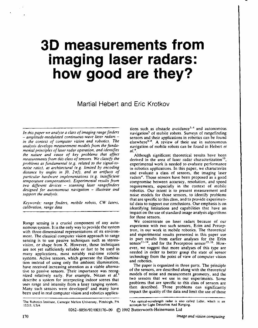
Figure 1 illustrates the reference frame. As shown, the y-axis coincides with the direction of travel of the laser beam projected through the central point of the scanner (i.e. the principal ray). The angle 8 (azimuth) corresponds to a rotation about the z-axis. The angle q (elevation) corresponds to a rotation about the x-axis.

Given the sensor measurement ( u , v, d ) (i.e. row, column, range), the transformation to spherical-polar

2

t

0

L 8 J Azimuth

Figure 1. Reference frame for scanning laser range finder. R: denotes range. To be consistent wirh the majoriry of the text, we should denote range by r

171

coordinates is:

p = u A . + p o , 8 = v A e + 8 , , r = A R d (1)

where:

A v is the angular increment, in degreedrow, of the nodding mirror, A e is the angular increment, in degreedcolumn, of the panning mirror, p, is the initial orientation, in degrees, of the nodding mirror, 8, is the initial orientation, in degrees, of the panning mirror, and A R is the scanner range resolution in metreslgrey- level.

Given the spherical polar coordinates 9, 8, r , the transformation to Cartesian coordinates is given by:

x = r sin 8, y =rcos8cosp, z = r cos6 sinp (2)

Measurement models An am-cw range sensor would approach perfection if it emitted a zero-width laser beam and observed the returned signal through an infinitely small receiver. In reality, the beam subtends a non-zero angle, and the receiver detects signals subtended by a solid angle we will call the instantaneous field of view (IFOV). Assuming a circular field stop, the beam projects to an ellipse on the target surface, the footprint of the beam. Every point within the intersection of the footprint and the IFOV contributes a range value and an intensity value to the final range and intensity measurements.

We may model a (range, intensity) pair as a complex number I, or equivalently as a vector (see Figure 2a). The phase of z represents the sensed range (or phase shift), and the magnitude of z is the sensed intensity. According to this model, the range measured at a pixel is the integral of k o z over the IFOV of the receiver, where ko is scalar and depends on parameters of the instrument (transmitted power, and the electro-optics of the receiver) and parameters of the environment (the angle a between the surface normal and the direction of measurement, the reflectance p of the target surface, and the range r as shown in Figure 2b).

Ultimately, the fidelity of the range measurement depends on the power of the signal reaching the photodetector, which in turn depends on ko. More precisely, the time-average radiant flux F (in watts) reaching the photodetector can be shown"to be:

(3)

Figure 2. Model of (range, intensity) pair as complex number

where k , is a function of the transmitted radiant flux, the capture area of the receiver, and filter bandwidths. Assuming that the output power of the photodetector is proportional to Fp, the output signal is proportional to p cos alr '.

When the received power is small, the output signal is small, and noise is significant. There are many sources of noise, including photon noise, laser noise, ambient noise, dark-current noise, secondary emission noise, and subsequent amplifier noise.

Nitzan et al.' identify photon noise as the dominant source, and assume that photoemission is a Poisson process to obtain the signal-to-noise ratio:

S N R = k 2 ( 7 ) pcosa ' R (4)

Assuming a modulation index of 100%, they go on to derive the approximate effect of photon noise on the measured range value. Their analysis indicates that the standard deviation of the range can be estimated by:

Combining (4) and ( 5 ) yields:

where the first term depends only on the physical, optical, and electronic characteristics of the sensor, and the second term depends only on the observed scene.

This equation states that or is approximately linear in r . or equivalently, that the variance vf is approximately quadratic in r . Our experimental results follow this model. In particular, Figure 12 shows that os is quadratic in r , consistent with (6 ) .

Examples We used two sensors for experiments: Erim and Perceptron, whose geometric parameters are listed in Table 1. Other sensors based on the same principle exist2*18. The two sensors that we use are typical of the operation and performance of this type of sensor.

The Erim scanning laser rangefinder is designed for applications in outdoor autonomous navigation. Several versions of the scanner exist. We refer to the version used for research on autonomous land

Table 1. Nominal values of sensor parameters

Parameter Units Erim Perceprron Descriprion

WfO" deg 30 60 Vertical FOV @/O" deg 80 60 Horizontal FOV N,O, pixel 64 256 Rows N C O , pixel 256 256 Columns A v A e

N bit 8 12 Number of bitslpixel Ail - 3.0in 0.98crn Range unit'

deg 0.47 0.24 Vertical step' deg 0.32 0.24 - 64ft 40rn

Horizontal stepZ Ambiguity interval ra

172 image and vision comDutinp

Figure 3. €rim intensity (top) and range images. The scene contains a tree (visible to the left), and a person (visible in the upper centre) on a path

n a v i g a t i ~ n ~ , ~ , which is the successor of a sensor used for legged loc~motion.'~.

The Erim scanner used a l00mW laser diode operating at 830 nm. The sensor volume is roughly 90 x x90cm, and the mass is about 45kg. The scanning mechanism consists of a vertical rotating mirror for horizontal scanning, and a horizontal nodding mirror for vertical scanning. The acquisiton rate is 0.5s for a 63x256 x 8 bit image. Table 1 summarizes the characteristics of the sensor. Figure 3 shows a range image (bottom) and a reflectance image (top) from the Erim scanner. The images show an outdoor scene of a road surrounded by a few trees. The sharp disconti- nuity at the top of the range image is due to the ambiguity interval of about 20m.

The Perceptron scanning laser range finder is more recent than the Erim, and has higher resolution and bandwidth. It is currently used for terrain mapping in support of legged locomotion*'.

The sensor volume is roughly 5Ox45x35cm, and the mass is about 30kg. The sensor uses a 180mW laser diode operating at 810nm. The image acquisition rate is 0.5s for a 2 5 6 x 2 5 6 ~ 12 bit image. The scanning mechanism is similar to the Erim design, except that the vertical field of view and the vertical image size are programmable. Table 1 summarizes the operating characteristics of the sensor as specified by the manufacturerI6.

Figure 4 shows the eight most significant bits of a

typical range image (right) and intensity image (left) from the Perceptron. The distance between the scanner and the floor is approximately 4m.

PROBLEMS In this section we describe four effects that may lead to corrupted or degraded data. Two effects, mixed pixels and rangehntensity crosstalk, are due to fundamental limitations of am-cw laser radars, although they are sometimes compounded with problems in the design of the actual sensors that we used. The two other effects, distortion due to scanning and range drift, are more specific to the particular sensors that we use. However, it is important to be aware of those effects since they do affect the quality of the data. Furthermore, simple cost- effective remedies do not seem to exist at the moment even though those problems are theoretically avoidable.

Mixed pixels Significant problems occur at pixels that receive reflected energy from two surfaces separated by a large distance. From an image analysis point of view, we would like the range at such points to be measured on either of the surfaces, or at least to fall in between in some predictable way. The fact that the range is measured by integrating over the entire projected spot leads to a phenomenon known as mixed pixels in which the measured range can be anywhere along the line of sight. In practical terms, this means that occluding edges of scene objects are unreliable, and that phantom objects may appear due to mixed measurements that are far from the real surfaces. This is a problem inherent to direct detection am-cw laser radars and i t cannot be completely eliminated.

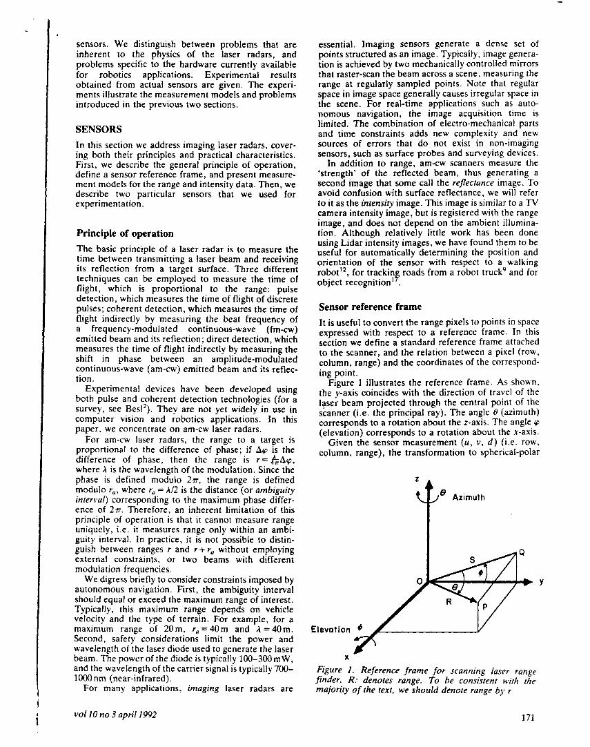
Figure 5 shows the geometry of the measurement at an occluding edge: two objects at distances D 1 and D, from the sensor (Dl < D2) are separated by a distance D, and a point is measured at the edge between the two surfaces. Due to the angular width of the beam, the range is formed by integration over a spot that contains reflections from both surfaces. The relevant parameter is the ratio p between the spot surface due to the near

Figure 4. Perceptron intensity (lefr) and range images. One of the authors is visible in the intensity image standing in front of box-like targets used for calibrat- ing the sensor. The images have been enhanced for printing

V O ~ 10 no 3 april1992 173

n

D - D1 c D2

Figure 5. Surface 1 occludes surface 2 (wide view)

surface and the total area. The combination of the two measurements is better explained using a model in the complex plane like the one presented below. Each portion i of the spot generates a measurement that can be represented by a complex number zi. The phase of zl, (oI is proportional to the range D,, and its magnitude depends on the reflectivity p, of the material. The resulting measurement is given by the sum t = z1 + z2. The finally measured range is proportional to the phase of z.

The phenomenon becomes clear with this formulation: the phase of z can be anywhere between (ol and cp2, depending on the ratio of the lengths of zI and z2 which depends on p , p l , and p2. The effect of mixing on sensed range becomes even more unpredictable when D is greater than half the ambiguity interval of the sensor. In that case, the angle cp between zl and z2 is greater than m, and the resulting measurement is such that q z < p < 2 n or O < (o < cpl, depending on p and the reflectivities. In the first case, the range may be anywhere behind the furthest object. In the second case, the range may be anywhere in front ofthe nearest object. In practice, the latter situation occurs only in specific combinations of range and scene geometry. In practice, this phenomenon is observed as soon as there are discrete objects in the scene. Figure 6 shows the effect of mixed pixels in a real image. The top panel shows an Erim image with a small window (shown as a white rectangle) containing an object (a tree) and its left and right edges. The bottom panel shows an overhead view of the I?D points in this region as calculated by Equation (2), and using the range from the image pixels. The points at the centre of the distribution correspond to the smooth surface of the object. Away from the centre are two lines of mixed pixels that appear at the object’s edges. In this example, all mixed pixels are located between the two targets, tree and background surface. This result is typical of the mixing effect in laser radars.

;. ‘

. .:‘ .l,i;;y.

Figure 6. Mixed pixels in real image. Top: selected region in Erim image; bottom: overhead view of the corresponding points

The mixed pixel effect complicates the processing and interpretation of the range images. Its main consequence is that strong range edges are unreliable. One approach to the problem is to apply a median filter to the image. The filter removes most of the mixed pixels since they appear as spurious readings only along the direction of an edge. Another approach is to transform all the points to a 3D coordinate frame. There, mixed pixels appear as isolated points, which makes them easier to remove than in image space. Since these two approaches remove mixed pixels whose range is far from the true value, they will not remove those in the vicinity of the actual edge. Thus, it is not possible for them to remove reliably all the mixed pixels from the data.

Scanning pattern With currently available commercial technology, imaging can be achieved only by scanning the beam using rotating and nodding mirrors. The scanning mechanism introduces additional errors into the sensor. They are probably the hardest to quantify and to correct. We identify three sources of error: synchronization, distortion, and localization. They result in a correct range measurement being stored at the wrong pixel in the image. Limitations due to the scanning mechanism are not inherent to the am-cw technology, but are due to the lack of alternatives to electro-mechanical scanning devices.

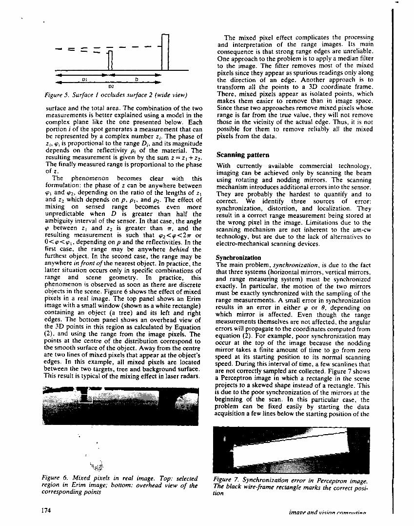
Synchronization The main problem, synchronization, is due to the fact that three systems (horizontal mirrors, vertical mirrors, and range measuring system) must be synchronized exactly. In particular, the motion of the two mirrors must be exactly synchronized with the sampling of the range measurements. A small error in synchronization results in an error in either cp or 8, depending on which mirror is affected. Even though the range measurements themselves are not affected, the angular errors will propagate to the coordinates computed from equation (2). For example, poor synchronization may occur at the top of the image because the nodding mirror takes a finite amount of time to go from zero speed at its starting position to its normal scanning speed. During this interval of time, a few scanlines that are not correctly sampled are collected. Figure 7 shows a Perceptron image in which a rectangle in the scene projects .to a skewed shape instead of a rectangle. This is due to the poor synchronization of the mirrors at the beginning of the scan. In this particular case, the problem can be fixed easily by starting the data acquisition a few lines below the starting position of the

Figure 7. Synchronization error in Perceptron image. The black wire-frame rectangle marks the correct posi- tion

174 imaee and virinn rnmnirtinn

nodding mirror. In general, i t is not possible to perfectly synchronize the mirrors. In general, there is a discrepancy between the nominal values of the scanning angles and the actual values. This error is difficult to quantify. We describe an experimental setup for estimating the angular error distribution later.

The distribution of the scanning errors due to poor synchronization remains relatively constant as long as the sensor is stationary. The effect of them on the image may be predicted, and appropriate corrections can be made by simple processing of the range images. For example, ignoring the first few rows would eliminate most of the unreliable measurements. However, additional image distortion may occur in some applications. In autonomous navigation applica- tions, for example, the sensor may be subject to motion, shocks and vibrations. This may produce large errors in scanning angles because of the mirrors getting out of phase. Those errors are hard to quantify. This effect is unavoidable except through the use of an external stabilization device.

The distribution of the scanning errors due to poor synchronization remains relatively constant as long as the sensor is stationary. However, additional image distortion may occur in some applications in which the scanner is subject to external motion.

Localization Even with perfect synchronization and no distortion due to external motion, sensor geometry may be incorrect if one uses a simplified model of the scanning mechanism. The ideal geometric model given above assumes implicitly that all the directions of measurements originate from a single point. This is equivalent to saying that the mirrors are infinitely small and are located exactly at the same point. Some dimension and do not coincide in space. Therefore, the measurement directions do not intersect at a single point. In reality, the measurements intersect along a line instead of intersecting at a point. This is a problem of localization of the origin of the sensor which translates into a systematic error in the conversion from (r, 8, cp) to (x, y, 2 ) . It could be solved by modelling the scaning mechanism or by calibration. For medium- range scanners such as Perceptron and Erim, the localization error is small compared to the errors on range and scanning angles.

intensities that can be observed. As a result, surfaces that reflect intensities outside of the optimal operating range will produce noisy or even erroneous range measurements. This effect can be reduced by dynamically adjusting the operating range according to the intensity. The Perceptron scanner implmements such a solution. However, the low intensities (dropout) and the high intensities (saturation) still produce spurious range readings. There are ways to increase the dynamic range of the receiver but they are not implemented in most scanners available to date.

The crosstalk effect becomes more noticeable at edges or on textured surfaces. In those cases, the beam illuminates a region that contains points of different surface reflectance. Since those points may generate slightly different range measurements, the situation is similar to the one discussed above, exxept that the mixing is due to the variation of reflectance within the spot instead of the variation of range. A consequence of this effect is that the behaviour of the range measurement at the edge between two surfaces with different reflectance may be unpredictable.

The crosstalk problem cannot be completely eliminated. However, some additions to the basic sensor design can diminish its effects. For example, the Perceptron scanner adjusts dynamically the operating range of the receiver, and uses a lookup table built using an off-line calibration procedure to correct the range as a function of intensity.

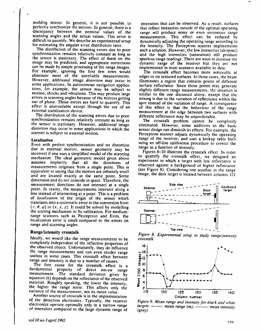
Figures 8-10 illustrate the crosstalk effect. In order to quantify the crosstalk effect, we designed an experiment in which a target with low reflectance is observed against a background of higher reflectance (see Figure 8). Considering one scanline in the range image, the dark target is located between columns 121

sc r

Rangehntensity crosstalk Ideally, we would like the range measurements to be completely independent of the reflective properties of the observed object. Unfortunately, they do influence rhe range measurements and can even render range useless in some cases. This crosstalk effect between range and intensity is due to a number of causes.

The first cause for the crosstalk effect is a fundamental property of direct am-cw range measurement. The standard deviation given by equation (6) depends on the reflectance of the observed material. Roughly speaking, the lower the intensity, the higher the range noise. This affects only the variance of the measurement, not its mean value.

Another source of crosstalk is in the implementation of the detection electronics. Typically, the receiver electronics operate optimally only in a narrow range of intensities compared to the large dynamic range of

Figure 8. Experimental setup io study rangelin rensiry crosstalk

l6 14 c .. . n

(, ...*-..*

I I5 120 125 130 135 140 Column number

Figure 9. Mean range and intensity for black and white targets, -e . mean range (m); -----. . mean inrensity (grey)

vol20 no 3 april1992 172

50r

l

- - - - a -

125 130 135 140 120 Column

Figure I O . Variance of range and intensity for black and white targets. -. . variance of range (cm2); -----: variance of intensity (grey ')

and 135. We computed the mean and variance of the range and intensity distributions at each pixel in the scanline by taking 100 images of the scene. Figure 9 shows the mean values as a function of the column number. The mean intensity drops sharply at the edges of the black target and remains at a low level between them, as expected. The mean range remains roughly constant except for a sharp discontinuity at each edge. The reason is that the intensity from both materials is mixed at the edges, therefore the range is not properly corrected. Figure 10 shows the variance of the range and intensity distributions. This clearly shows a sharp increase in d between the high intensity background and the black target, as expected from the theoretical expression of range noise.

Range drift We observed a significant drift of range measurements over time. To illustrate this effect, we placed a target 6 m from the origin of the Perceptron scanner and acquired one image per minute over 24 hours, during which the scene was static.

Figure 11 plots the sensed range at one target pixel. The figure shows a dramatic variation over time. Between hours 0 and 3, the ranges climb approximately one metre, as if the sensor were translating away from the target. After this four hour 'warm-up' period, the sensed ranges reach a plateau where they remain, with apparently random variations, for the rest of the day.

We hypothesized that some of the variations might be due to temperature changes. To test this hypothesis, we placed an electric heater directly behind the scanner, and repeated the above trial, acquiring images

Time (hours) Figure 11. Range measurements vary over time. The target is a sheet of cardboard 6 m in front of the scanner

176

at 2 H z over two hours (14,000 images). Without the heater, the temperature was 21"C, and we observed approximately constant range measurements. We turned on the heater and after 30 minutes the temperature climbed to 45°C. During this time, the sensed ranges fell about N c m , a substantial decline. When we turned off the heater, the sensed ranges gradually increased until they regained their original level. This demonstrates conclusively that the temperature changes cause the distribution of range values to translate by significant amounts.

It is clear that heat cannot directly affect the phase shift which carries the range information. Therefore, the drift observed in those experiments is due to poor temperature compensation in the electronics used in the scanner. Improvements in the electronics have reduced this effect considerably. An important lesson is that such effects may dominate the errors due to the physics of the measurements.

ACCURACY AND PRECISION We have introduced a theoretical framework that leads to a characterization of expected sensor accuracy for am-cw laser radars. However, it is important to verify that the sensors do indeed follow the theoretical model. In particular, real sensors include effects such as those described above that are not part of the theoretical framework. Actual sensor accuracy is important in determining what algorithms and what applications are appropriate for a given sensor. In this section we describe a series of experiments designed to measure range accuracy for the Erim and Perceptron sensors under different conditions and to compare it with the predicted theoretical values. Following Besl', we dis- tinguish between accuracy, the difference between measured range and actual range, and precision, the variation of measured range to a given target. To separate the errors due to scanning and the errors due to actual range measurements, we distinguish between range precision and angular precision.

Accuracy To determine the accuracy of the range measurements is to identify the distance between them and ground truth ranges. For a target point lying in the direction (cp, e), let rv,e be the range measurement reported by the scanner, and let dv.e be the true distance from the geometric origin, measured with a tape measure. Under ideal conditions, we expect to observe a linear relationship:

where ro is the offset distance from the origin to the (conceptual) surface corresponding to a range measure- ment of zero, and a is the slope.

To determine the parameters a and ro, we acquire range measurements of targets at six known distances between 6 and 16m. and fit a line to the data. We illustrate the results for the Perceptron scanner in Table 2, which shows the extracted parameters from five trials under different conditions. Because of range drift (c.f. above), we do not assign high confidence to the

image and vision comnutinp

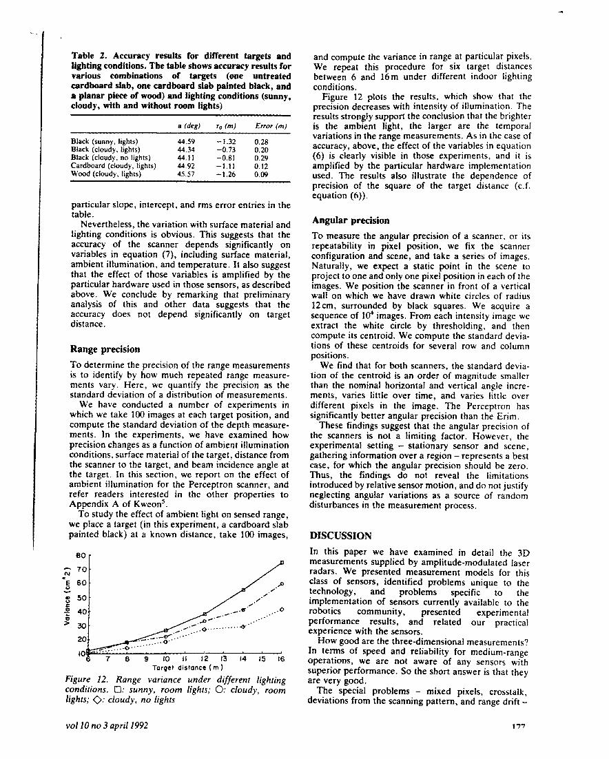
Table 2. Accuracy results for different targets and lighting conditions. The table shows accuracy results for various combinations of targets (One untreated cardboard slab, one cardboard slab painted black, and a planar piece of wood) and lighting conditions (sunny, cloudy, with and without room lights)

Black (sunny, lights) 44.59 -1.32 0.28 Black (cloudy, lights) 44.34 -0.73 0.20 Black (cloudy, no lights) 44.11 -0.81 0.29

Wood (cloudy, lights) 45.57 -1.26 0.09 Cardboard (cloudy, lights) 44.92 - 1 . 1 1 0.12

particular slope, intercept, and rms error entries in the table.

Nevertheless, the variation with surface material and lighting conditions is obvious. This suggests that the accuracy of the scanner depends significantly on variables in equation (7), including surface material, ambient illumination, and temperature. It also suggest that the effect of those variables is amplified by the particular hardware used in those sensors, as described above. We conclude by remarking that preliminary analysis of this and other data suggests that the accuracy does not depend significantly on target distance.

Range precision To determine the precision of the range measurements is to identify by how much repeated range measure- ments vary. Here, we quantify the precision as the standard deviation of a distribution of measurements.

We have conducted a number of experiments in which we take 100 images at each target position, and compute the standard deviation of the depth measure- ments. In the experiments, we have examined how precision changes as a function of ambient illumination conditions, surface material of the target, distance from the scanner to the target, and beam incidence angle at the target. In this section, we report on the effect of ambient illumination for the Perceptron scanner, and refer readers interested in the other properties to Appendix A of Kweon’.

To study the effect of ambient light on sensed range, we place a target (in this experiment, a cardboard slab painted black) at a known distance, take 100 images,

Torget distance ( m )

Figure 12. Range variance under different lighting conditions. 0: sunny, room lights; 0: cloudy, room lights; 0: cloudy, no lights

and compute the variance in range at particular pixels. We repeat this procedure for six target distances between 6 and 16m under different indoor lighting conditions.

Figure 12 plots the results, which show that the precision decreases with intensity of illumination. The results strongly support the conclusion that the brighter is the ambient light, the larger are the temporal variations in the range measurements. As in the case of accuracy, above, the effect of the variables in equation (6) is clearly visible in those experiments, and it is amplified by the particular hardware implementation used. The results also illustrate the dependence of precision of the square of the target distance (c.f. equation (6)).

Angular precision To measure the angular precision of a scanner, or its repeatability in pixel position, we fix the scanner configuration and scene, and take a series of images. Naturally, we expect a static point in the scene to project to one and only one pixel position in each of the images. We position the scanner in front of a vertical wall on which we have drawn white circles of radius 12cm, surrounded by black squares. We acquire a sequence of 104 images. From each intensity image we extract the white circle by thresholding, and then compute its centroid. We compute the standard devia- tions of these centroids for several row and column positions.

We find that for both scanners, the standard devia- tion of the centroid is an order of magnitude smaller than the nominal horizontal and vertical angle incre- ments, varies little over time, and varies little over different pixels in the image. The Perceptron has significantly better angular precision than the Erim.

These findings suggest that the angular precision of the scanners is not a limiting factor. However, the experimental setting - stationary sensor and scene, gathering information over a region - represents a best case, for which the angular precision should be zero. Thus, the findings do not reveal the limitations introduced by relative sensor motion, and do not justify neglecting angular variations as a source of random disturbances in the measurement process.

DISCUSSION In this paper we have examined in detail the 3D measurements supplied by amplitude-modulated laser radars. We presented measurement models for this class of sensors, identified problems unique to the technology, and problems specific to the implementation of sensors currently available to the robotics community, presented experiment a1 performance results, and related our practical experience with the sensors.

How good are the three-dimensional measurements? In terms of speed and reliability for medium-range operations, we are not aware of any sensors with superior performance. So the short answer is that they are very good.

The special problems - mixed pixels, crosstalk, deviations from the scanning pattern, and range drift -

vol IO no 3 uprif I992 177

make i t necessary to pre-process the images. For some problems (e.g. mixed pixels) no solutions exist. Thus, range data interpretation algorithms, like so many others in machine perception, must tolerate spurious data.

The quantitative performance, in terms of accuracy and precision, is highly variable. It depends on geometric factors such as incidence angle and target distance. We understand these reasonably well. But it also depends significantly on non-geometric factors such as temperature, ambient illumination, and surface material type. Even though detailed measurement models which include some of those variables have been developed, there is still a significant discrepancy between the theoretical sensor characteristics and the observed performance.

ACKNOWLEDGEMENTS The authors wish to thank M. Blackwell, R. Hoffman, and 1. Kweon who performed many of the experiments described in this paper and kept the scanners in working condition. This work was supported in part by NASA under Grant NAGW-1175 and by DARPA through ARPA No. 4976 monitored by the Air Force Avionics Laboratory under contract F33615-87-C-1499. The views and conclusions contained in this document are those of the authors and should not be interpreted as representing the policies of NASA, DARPA, or the US government.

REFERENCES 1 Nitzan, D, Brain, A and Duda, R ‘The

measurement and use of registered reflectance and range data in scene analysis’, Proc. IEEE, Vol 65 No 2 (February 1977) pp 206-220

2 Bel , P ‘Active, optical range imaging sensors’, Machine Vision & Applications, Vol 1 (1988) pp

3 Dunlay, R and Morgenthaler, D ‘Obstacle detection and avoidance from range data’, Proc. SPIE Mobile Robots Conf., Cambridge, MA (1986)

4 Veatch, P and Davis, L ‘Efficient algorithms for obstacle detection using range data’, Comput. Vision, Graph. & Image Process., Vol50 (1990) pp

5 Kweon, I Modeling Rugged Terrain with Multiple Sensors, PhD thesis, School of Computer Science, Carnegie Mellon University (January 1991)

127-152

50-71

6

7

8

9

10

11

12

13

14

15

16

17

18

19

20

Everett, H ’Survey of collision avoidance and ranging sensors for mobile robots’, Robotics & Autonomous Syst., Vol 5 (1989) pp 5-67 Jain, R and Jain, A Analysis and Interpretation of Range Images, Springer-Verlag, New York (1990) Nitzan, D ‘Assessment of robotic sensors’, Proc. fnt. Conf. Robot Vision and Sensory Controls, London, UK (April 1981) pp 1-11 Hebert, M, Kanade, T and Kweon, 1 3 - 0 Vision Techniques for Autonomous Vehicles, Technical Report CMU-RI-TR-88-12, Robotics Institute, Carnegie Mellon University (August 1988) Pratt, W Laser Communication Systems, Wiley, New York (1969) Environmental Research Institute of Michigan, Proc. Range and Reflectance Processing Workshop, Ann Arbor, MI (1987, limited distribu- tion) Krotkov, E Laser Rangefinder Calibration for a Walking Robot, Technical Report CMU-RI-TR- 90-30, Robotics Institute, Carnegie Mellon Uni- versity (December 1990) Watts, R, Pont, F and Zuk, D Characterization of the ERIMIA LV Sensor - Range and Reflectance, Technical Report, ERIM, Ann Arbor, MI (1987) Zuk, D, Pont, F, Franklin, R and Larrowe, V A System for Autonomous Land Navigation, Tech- nical Report IR-85-540, ERIM, Ann Arbor, MI (1985) Kweon, I, Hoffman, R and Krotkov, E Experi- mental Characterization of the Perceptron Laser Rangefinder, Technical Report CMU-RI-TR-91-1, Robotics Institute, Carnegie Mellon University (January 1991) Perceptron, Inc., Farmington Hills, Michigan, LIDAR Scanning System (U.S. Patent Appl. No.

Hebert, M and Kanade, T ‘3-D vision for outdoor navigation by an autonomous vehicle’, Proc. Image Understanding Workshop, Cambridge, MA ( 1988) Odetics, Inc., Anaheim, California 3 0 Laser Imaging System ( 1989) Zuk, D and Delleva, M Three-Dimensional Vision Sysrem for the ASV, Final Report No. 170400-3-f, DARPA, Defense Supply Service, Washington (January 1983) Hebert, M, Krotkov,- E and Kanade, T ‘A Perception system for a planetary explorer’, Proc. IEEE Con$ on Decision and Control, Tampa, FL (December 1989) pp 1151-1156

4226-00015)

178