2danniversaryedition 1 tutorial
DESCRIPTION
plaxisTRANSCRIPT
7/21/2019 2DAnniversaryEdition 1 Tutorial
http://slidepdf.com/reader/full/2danniversaryedition-1-tutorial 1/176
PLAXIS 2D
Tutorial Manual
Anniversary Edition

7/21/2019 2DAnniversaryEdition 1 Tutorial
http://slidepdf.com/reader/full/2danniversaryedition-1-tutorial 2/176
7/21/2019 2DAnniversaryEdition 1 Tutorial
http://slidepdf.com/reader/full/2danniversaryedition-1-tutorial 3/176
TABLE OF CONTENTS
TABLE OF CONTENTS
1 Settlement of a circular footing on sand 7
1.1 Geometry 7
1.2 Case A: Rigid footing 81.3 Case B: Flexible footing 22
2 Submerged construction of an excavation 29
2.1 Input 30
2.2 Mesh generation 35
2.3 Calculations 36
2.4 Results 40
3 Dry excavation using a tie back wall 43
3.1 Input 43
3.2 Mesh generation 483.3 Calculations 48
3.4 Results 54
4 Construction of a road embankment 57
4.1 Input 57
4.2 Mesh generation 61
4.3 Calculations 61
4.4 Results 65
4.5 Safety analysis 67
4.6 Using drains 724.7 Updated mesh + Updated water pressures analysis 73
5 Settlements due to tunnel construction 75
5.1 Input 75
5.2 Mesh generation 80
5.3 Calculations 81
5.4 Results 83
6 Excavation of an NATM tunnel 87
6.1 Input 87
6.2 Mesh generation 916.3 Calculations 91
6.4 Results 94
7 Stability of dam under rapid drawdown 97
7.1 Input 97
7.2 Mesh generation 98
7.3 Calculation 99
7.4 Results 107
8 Dry excavation using a tie back wall - ULS 111
8.1 Input 111
8.2 Calculations 113
8.3 Results 114
PLAXIS 2D Anniversary Edition | Tutorial Manual 3

7/21/2019 2DAnniversaryEdition 1 Tutorial
http://slidepdf.com/reader/full/2danniversaryedition-1-tutorial 4/176
TUTORIAL MANUAL
9 Flow through an embankment 117
9.1 Input 117
9.2 Mesh generation 118
9.3 Calculations 119
9.4 Results 123
10 Flow around a sheet pile wall 127
10.1 Input 127
10.2 Mesh generation 127
10.3 Calculations 128
10.4 Results 129
11 Potato field moisture content 131
11.1 Input 131
11.2 Mesh generation 133
11.3 Calculations 13411.4 Results 137
12 Dynamic analysis of a generator on an elastic foundation 139
12.1 Input 139
12.2 Mesh generation 141
12.3 Calculations 142
12.4 Results 146
13 Pile driving 149
13.1 Input 149
13.2 Mesh generation 15313.3 Calculations 153
13.4 Results 156
14 Free vibration and earthquake analysis of a building 159
14.1 Input 159
14.2 Mesh generation 164
14.3 Calculations 165
14.4 Results 167
Appendix A - Menu tree 171
4 Tutorial Manual | PLAXIS 2D Anniversary Edition

7/21/2019 2DAnniversaryEdition 1 Tutorial
http://slidepdf.com/reader/full/2danniversaryedition-1-tutorial 5/176
INTRODUCTION
INTRODUCTION
PLAXIS is a finite element package that has been developed specifically for the analysis
of deformation and stability in geotechnical engineering projects. The simple graphical
input procedures enable a quick generation of complex finite element models, and theenhanced output facilities provide a detailed presentation of computational results. The
calculation itself is fully automated and based on robust numerical procedures. This
concept enables new users to work with the package after only a few hours of training.
Though the various tutorials deal with a wide range of interesting practical applications,
this Tutorial Manual is intended to help new users become familiar with PLAXIS 2D. The
tutorials should therefore not be used as a basis for practical projects.
Users are expected to have a basic understanding of soil mechanics and should be able
to work in a Windows environment. It is strongly recommended that the tutorials are
followed in the order that they appear in the manual. Please note that minor differences inresults maybe found, depending on hardware and software configuration.
The Tutorial Manual does not provide theoretical background information on the finite
element method, nor does it explain the details of the various soil models available in the
program. The latter can be found in the Material Models Manual, as included in the full
manual, and theoretical background is given in the Scientific Manual. For detailed
information on the available program features, the user is referred to the Reference
Manual. In addition to the full set of manuals, short courses are organised on a regular
basis at several places in the world to provide hands-on experience and background
information on the use of the program.
PLAXIS 2D Anniversary Edition | Tutorial Manual 5

7/21/2019 2DAnniversaryEdition 1 Tutorial
http://slidepdf.com/reader/full/2danniversaryedition-1-tutorial 6/176
TUTORIAL MANUAL
6 Tutorial Manual | PLAXIS 2D Anniversary Edition

7/21/2019 2DAnniversaryEdition 1 Tutorial
http://slidepdf.com/reader/full/2danniversaryedition-1-tutorial 7/176
SETTLEMENT OF A CIRCULAR FOOTING ON SAND
1 SETTLEMENT OF A CIRCULAR FOOTING ON SAND
In this chapter a first application is considered, namely the settlement of a circular
foundation footing on sand. This is the first step in becoming familiar with the practical
use of PLAXIS 2D. The general procedures for the creation of a geometry model, thegeneration of a finite element mesh, the execution of a finite element calculation and the
evaluation of the output results are described here in detail. The information provided in
this chapter will be utilised in the later tutorials. Therefore, it is important to complete this
first tutorial before attempting any further tutorial examples.
Objectives:
• Starting a new project.
• Creating an axisymmetric model
• Creating soil stratigraphy using the Borehole feature.
• Creating and assigning of material data sets for soil (Mohr-Coulomb model ).
• Defining prescribed displacements.
• Creation of footing using the Plate feature.
• Creating and assigning material data sets for plates.
• Creating loads.
• Generating the mesh.
• Generating initial stresses using the K0 procedure.
• Defining a Plastic calculation.
• Activating and modifying the values of loads in calculation phases.
• Viewing the calculation results.
• Selecting points for curves.
• Creating a 'Load - displacement' curve.
1.1 GEOMETRY
A circular footing with a radius of 1.0 m is placed on a sand layer of 4.0 m thickness as
shown in Figure 1.1. Under the sand layer there is a stiff rock layer that extends to a large
depth. The purpose of the exercise is to find the displacements and stresses in the soil
caused by the load applied to the footing. Calculations are performed for both rigid and
flexible footings. The geometry of the finite element model for these two situations is
similar. The rock layer is not included in the model; instead, an appropriate boundary
condition is applied at the bottom of the sand layer. To enable any possible mechanism in
the sand and to avoid any influence of the outer boundary, the model is extended in
horizontal direction to a total radius of 5.0 m.
PLAXIS 2D Anniversary Edition | Tutorial Manual 7

7/21/2019 2DAnniversaryEdition 1 Tutorial
http://slidepdf.com/reader/full/2danniversaryedition-1-tutorial 8/176
TUTORIAL MANUAL
2.0 m
4.0 m
load
footing
x
y
sand
Figure 1.1 Geometry of a circular footing on a sand layer
1.2 CASE A: RIGID FOOTING
In the first calculation, the footing is considered to be very stiff and rough. In this
calculation the settlement of the footing is simulated by means of a uniform indentation at
the top of the sand layer instead of modelling the footing itself. This approach leads to a
very simple model and is therefore used as a first exercise, but it also has some
disadvantages. For example, it does not give any information about the structural forces
in the footing. The second part of this tutorial deals with an external load on a flexible
footing, which is a more advanced modelling approach.
1.2.1 GEOMETRY INPUT
Start PLAXIS 2D by double clicking the icon of the Input program. The Quick select
dialog box appears in which you can create a new project or select an existing one
(Figure 1.2).
Figure 1.2 Quick select dialog box
• Click Start a new project . The Project properties window appears, consisting of two
tabsheets, Project and Model (Figure 1.3 and Figure 1.4).
8 Tutorial Manual | PLAXIS 2D Anniversary Edition

7/21/2019 2DAnniversaryEdition 1 Tutorial
http://slidepdf.com/reader/full/2danniversaryedition-1-tutorial 9/176
SETTLEMENT OF A CIRCULAR FOOTING ON SAND
Project properties
The first step in every analysis is to set the basic parameters of the finite element model.
This is done in the Project properties window. These settings include the description of
the problem, the type of model, the basic type of elements, the basic units and the size of
the draw area.
Figure 1.3 Project tabsheet of the Project properties window
To enter the appropriate settings for the footing calculation follow these steps:
• In the Project tabsheet, enter "Lesson 1" in the Title box and type "Settlements of a
circular footing" in the Comments box.
• Click the Next button below the tabsheets or click the Model tab.
• In the Type group the type of the model (Model ) and the basic element type
(Elements ) are specified. Since this tutorial concerns a circular footing, select theAxisymmetry and the 15-Noded options from the Model and the Elements
drop-down menus respectively.
• Keep the default units in the Units group (Unit of Length = m; Unit of Force = kN;
Unit of Time = day).
• In the General group the unit weight of water (γ water ) is set to 10 kN/m3.
• In the Contour group set the model dimensions to x min = 0.0, x max = 5.0, y min = 0.0
and y max = 4.0.
Figure 1.4 Model tabsheet of the Project properties window
• Click OK button to confirm the settings.
PLAXIS 2D Anniversary Edition | Tutorial Manual 9

7/21/2019 2DAnniversaryEdition 1 Tutorial
http://slidepdf.com/reader/full/2danniversaryedition-1-tutorial 10/176
TUTORIAL MANUAL
Hint: In the case of a mistake or for any other reason that the project properties
need to be changed, you can access the Project properties window by
selecting the corresponding option from the File menu.
Definition of soil stratigraphy
When you click the OK button the Project properties window will close and the Soil mode
view will be shown where the soil stratigraphy can be defined.
Hint: The modelling process is completed in five modes. More information on
modes is available in the Section ?? of the Reference Manual.
Information on the soil layers is entered in boreholes. Boreholes are locations in the draw
area at which the information on the position of soil layers and the water table is given. If
multiple boreholes are defined, PLAXIS 2D will automatically interpolate between the
boreholes. The layer distribution beyond the boreholes is kept horizontal. In order to
construct the soil stratigraphy follow these steps:
Click the Create borehole button in the side (vertical) toolbar to start defining the soil
stratigraphy.
• Click at x = 0 in the draw area to locate the borehole. The Modify soil layers window
will appear.
• In the Modify soil layers window add a soil layer by clicking the Add button.
• Set the top boundary of the soil layer at y = 4 and keep the bottom boundary at y = 0
m.
• By default the Head value (groundwater head) in the borehole column is set to 0 m.
Set the Head to 2.0 m (Figure 1.5).
The creation of material data sets and their assignment to soil layers is described in the
following section.
Material data sets
In order to simulate the behaviour of the soil, a suitable soil model and appropriate
material parameters must be assigned to the geometry. In PLAXIS 2D, soil properties are
collected in material data sets and the various data sets are stored in a material
database. From the database, a data set can be assigned to one or more soil layers. For
structures (like walls, plates, anchors, geogrids, etc.) the system is similar, but different
types of structures have different parameters and therefore different types of material
data sets. PLAXIS 2D distinguishes between material data sets for Soil and interfaces ,
Plates , Geogrids , Embedded pile row and Anchors .
10 Tutorial Manual | PLAXIS 2D Anniversary Edition

7/21/2019 2DAnniversaryEdition 1 Tutorial
http://slidepdf.com/reader/full/2danniversaryedition-1-tutorial 11/176
SETTLEMENT OF A CIRCULAR FOOTING ON SAND
Figure 1.5 Modify soil layers window
To create a material set for the sand layer, follow these steps:
Open the Material sets window by clicking the Materials button in the Modify soil
layers window. The Material sets window pops up (Figure 1.6).
Figure 1.6 Material sets window
• Click the New button at the lower side of the Material sets window. A new window
will appear with five tabsheets: General , Parameters , Flow parameters , Interfaces
PLAXIS 2D Anniversary Edition | Tutorial Manual 11

7/21/2019 2DAnniversaryEdition 1 Tutorial
http://slidepdf.com/reader/full/2danniversaryedition-1-tutorial 12/176
TUTORIAL MANUAL
and Initial .
• In the Material set box of the General tabsheet, write "Sand" in the Identification box.
• The default material model (Mohr-Coulomb ) and drainage type (Drained ) are valid
for this example.• Enter the proper values in the General properties box (Figure 1.7) according to the
material properties listed in Table 1.1. Keep parameters that are not mentioned in
the table at their default values.
Figure 1.7 The General tabsheet of the Soil window of the Soil and interfaces set type
• Click the Next button or click the Parameters tab to proceed with the input of model
parameters. The parameters appearing on the Parameters tabsheet depend on the
selected material model (in this case the Mohr-Coulomb model).
• Enter the model parameters of Table 1.1 in the corresponding edit boxes of the
Parameters tabsheet (Figure 1.8). A detailed description of different soil models and
their corresponding parameters can be found in the Material Models Manual.
Figure 1.8 The Parameters tabsheet of the Soil window of the Soil and interfaces set type
12 Tutorial Manual | PLAXIS 2D Anniversary Edition

7/21/2019 2DAnniversaryEdition 1 Tutorial
http://slidepdf.com/reader/full/2danniversaryedition-1-tutorial 13/176
SETTLEMENT OF A CIRCULAR FOOTING ON SAND
Table 1.1 Material properties of the sand layer
Parameter Name Value Unit
General
Material model Model Mohr-Coulomb -
Type of material behaviour Type Drained -Soil unit weight above phreatic level γ unsat 17.0 kN/m3
Soil unit weight below phreatic level γ sat 20.0 kN/m3
Parameters
Young's modulus (constant) E ' 1.3 · 104 kN/m2
Poisson's ratio ν ' 0.3 -
Cohesion (constant) c 'ref 1.0 kN/m2
Friction angle ϕ' 30.0 ◦
Dilatancy angle ψ 0.0 ◦
• The soil material is drained, the geometry model does not include interfaces and the
default initial conditions are valid for this case, therefore the remaining tabsheets
can be skipped. Click OK to confirm the input of the current material data set. Nowthe created data set will appear in the tree view of the Material sets window.
• Drag the set Sand from the Material sets window (select it and hold down the left
mouse button while moving) to the graph of the soil column on the left hand side of
the Modify soil layers window and drop it there (release the left mouse button).
• Click OK in the Material sets window to close the database.
• Click OK to close the Modify soil layers window.
Hint: Existing data sets may be changed by opening the Material sets window,
selecting the data set to be changed from the tree view and clicking the Edit
button. As an alternative, the Material sets window can be opened by clicking
the corresponding button in the side toolbar.
» PLAXIS 2D distinguishes between a project database and a global database
of material sets. Data sets may be exchanged from one project to another
using the global database. The global database can be shown in the Material
sets window by clicking the Show global button. The data sets of all tutorials
in the Tutorial Manual are stored in the global database during the installation
of the program.
» The material assigned to a selected entity in the model can be changed in
the Material drop-down menu in the Selection explorer . Note that all thematerial datasets assignable to the entity are listed in the drop-down menu.
However, only the materials listed under Project materials are listed, and not
the ones listed under Global materials .
» The program performs a consistency check on the material parameters and
will give a warning message in the case of a detected inconsistency in the
data.
Visibility of a grid in the draw area can simplify the definition of geometry. The grid
provides a matrix on the screen that can be used as reference. It may also be used for
snapping to regular points during the creation of the geometry. The grid can be activated
by clicking the corresponding button under the draw area. To define the size of the grid
cell and the snapping options:
PLAXIS 2D Anniversary Edition | Tutorial Manual 13
7/21/2019 2DAnniversaryEdition 1 Tutorial
http://slidepdf.com/reader/full/2danniversaryedition-1-tutorial 14/176
TUTORIAL MANUAL
Click the Snapping options button in the side toolbar. The Snapping window pops
up where the size of the grid cells and the snapping interval can be specified. The
spacing of snapping points can be further divided into smaller intervals by the
Number of snap intervals value. Use the default values in this example.
Definition of structural elements
The structural elements are created in the Structures mode of the program where a
uniform indentation will be created to model a very stiff and rough footing.
• Click the Structures tab to proceed with the input of structural elements in the
Structures mode.
Click the Create prescribed displacement button in the side toolbar.
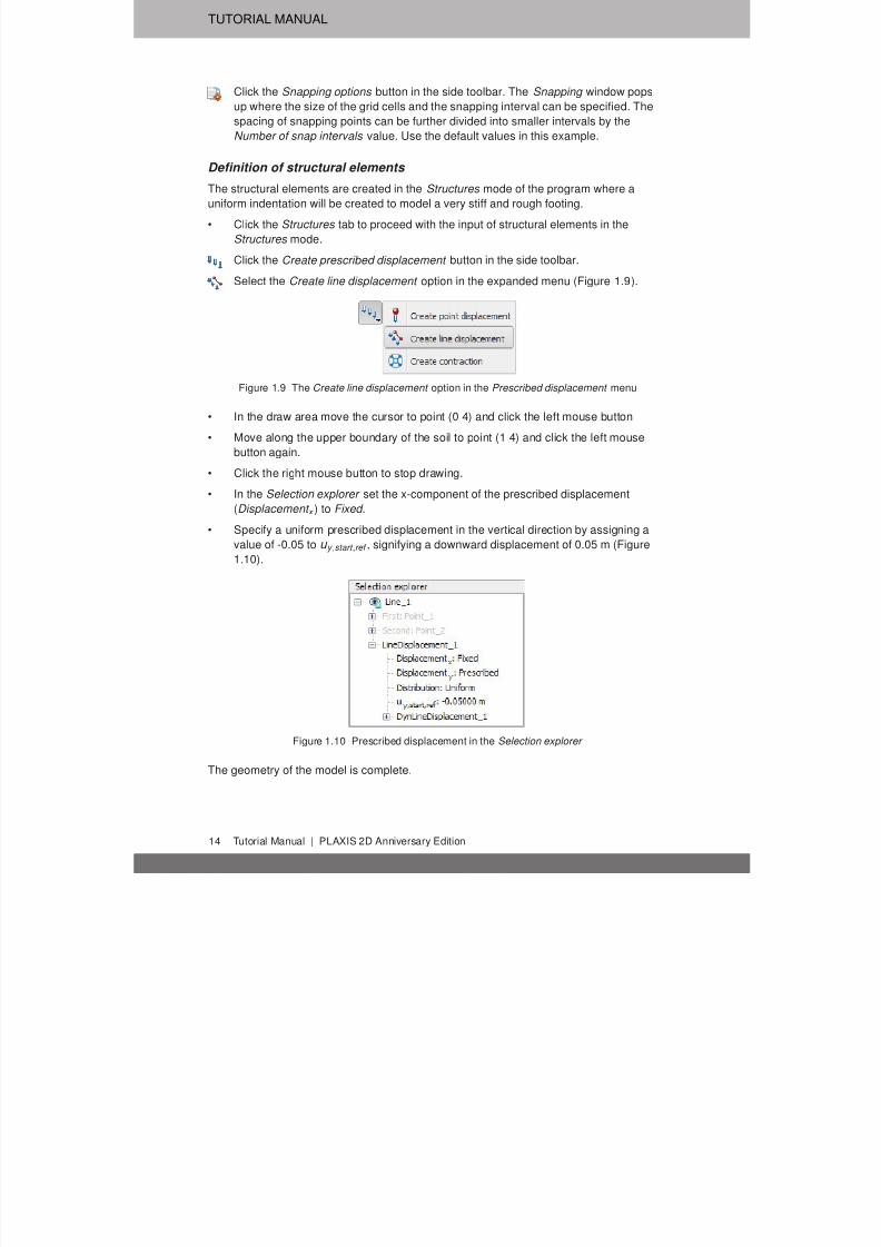
Select the Create line displacement option in the expanded menu (Figure 1.9).
Figure 1.9 The Create line displacement option in the Prescribed displacement menu
• In the draw area move the cursor to point (0 4) and click the left mouse button
• Move along the upper boundary of the soil to point (1 4) and click the left mouse
button again.
• Click the right mouse button to stop drawing.
• In the Selection explorer set the x-component of the prescribed displacement
(Displacement x ) to Fixed .
• Specify a uniform prescribed displacement in the vertical direction by assigning a
value of -0.05 to u y ,start ,ref , signifying a downward displacement of 0.05 m (Figure
1.10).
Figure 1.10 Prescribed displacement in the Selection explorer
The geometry of the model is complete.
14 Tutorial Manual | PLAXIS 2D Anniversary Edition
7/21/2019 2DAnniversaryEdition 1 Tutorial
http://slidepdf.com/reader/full/2danniversaryedition-1-tutorial 15/176
SETTLEMENT OF A CIRCULAR FOOTING ON SAND
Mesh generation
When the geometry model is complete, the finite element mesh can be generated.
PLAXIS 2D allows for a fully automatic mesh generation procedure, in which the
geometry is divided into elements of the basic element type and compatible structural
elements, if applicable.
The mesh generation takes full account of the position of points and lines in the model,
so that the exact position of layers, loads and structures is accounted for in the finite
element mesh. The generation process is based on a robust triangulation principle that
searches for optimised triangles. In addition to the mesh generation itself, a
transformation of input data (properties, boundary conditions, material sets, etc.) from the
geometry model (points, lines and clusters) to the finite element mesh (elements, nodes
and stress points) is made.
In order to generate the mesh, follow these steps:
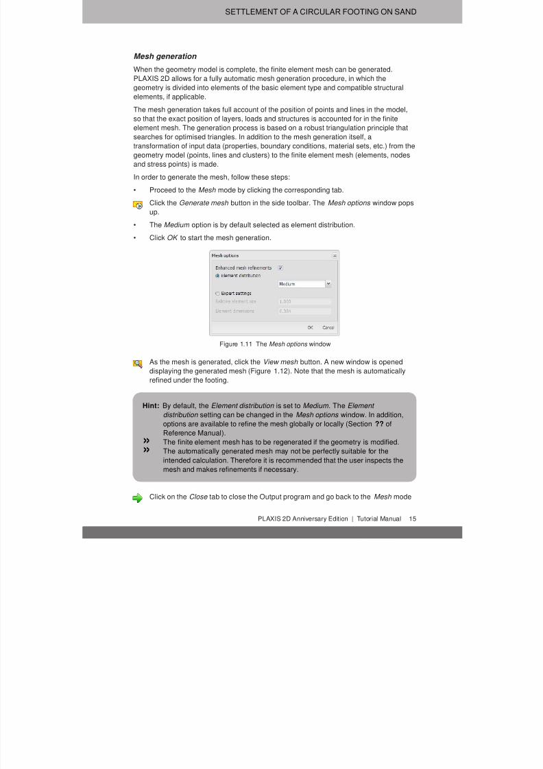
• Proceed to the Mesh mode by clicking the corresponding tab.
Click the Generate mesh button in the side toolbar. The Mesh options window pops
up.
• The Medium option is by default selected as element distribution.
• Click OK to start the mesh generation.
Figure 1.11 The Mesh options window
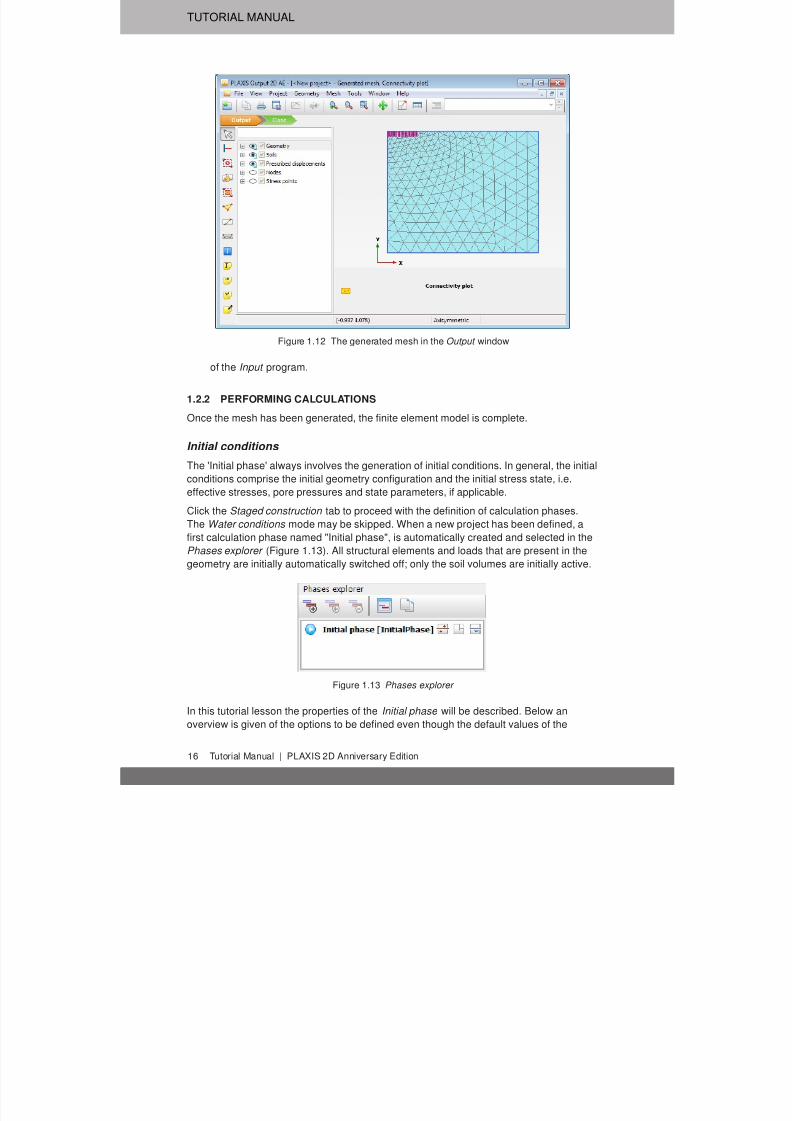
As the mesh is generated, click the View mesh button. A new window is opened
displaying the generated mesh (Figure 1.12). Note that the mesh is automatically
refined under the footing.
Hint: By default, the Element distribution is set to Medium . The Element
distribution setting can be changed in the Mesh options window. In addition,
options are available to refine the mesh globally or locally (Section ?? of
Reference Manual).
» The finite element mesh has to be regenerated if the geometry is modified.
» The automatically generated mesh may not be perfectly suitable for the
intended calculation. Therefore it is recommended that the user inspects the
mesh and makes refinements if necessary.
Click on the Close tab to close the Output program and go back to the Mesh mode
PLAXIS 2D Anniversary Edition | Tutorial Manual 15
7/21/2019 2DAnniversaryEdition 1 Tutorial
http://slidepdf.com/reader/full/2danniversaryedition-1-tutorial 16/176
TUTORIAL MANUAL
Figure 1.12 The generated mesh in the Output window
of the Input program.
1.2.2 PERFORMING CALCULATIONS
Once the mesh has been generated, the finite element model is complete.
Initial conditions
The 'Initial phase' always involves the generation of initial conditions. In general, the initial
conditions comprise the initial geometry configuration and the initial stress state, i.e.
effective stresses, pore pressures and state parameters, if applicable.
Click the Staged construction tab to proceed with the definition of calculation phases.
The Water conditions mode may be skipped. When a new project has been defined, a
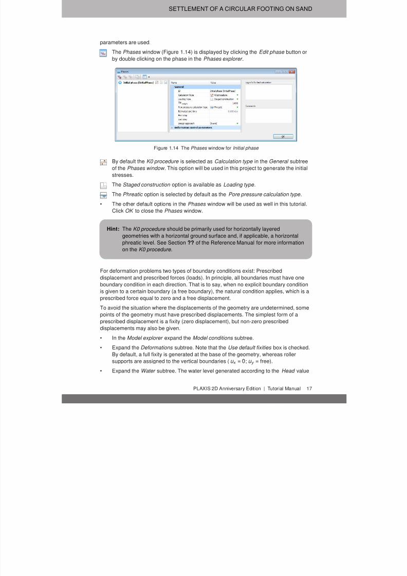
first calculation phase named "Initial phase", is automatically created and selected in the
Phases explorer (Figure 1.13). All structural elements and loads that are present in thegeometry are initially automatically switched off; only the soil volumes are initially active.
Figure 1.13 Phases explorer
In this tutorial lesson the properties of the Initial phase will be described. Below an
overview is given of the options to be defined even though the default values of the
16 Tutorial Manual | PLAXIS 2D Anniversary Edition
7/21/2019 2DAnniversaryEdition 1 Tutorial
http://slidepdf.com/reader/full/2danniversaryedition-1-tutorial 17/176
SETTLEMENT OF A CIRCULAR FOOTING ON SAND
parameters are used.
The Phases window (Figure 1.14) is displayed by clicking the Edit phase button or
by double clicking on the phase in the Phases explorer .
Figure 1.14 The Phases window for Initial phase
By default the K0 procedure is selected as Calculation type in the General subtree
of the Phases window . This option will be used in this project to generate the initial
stresses.
The Staged construction option is available as Loading type .
The Phreatic option is selected by default as the Pore pressure calculation type .
• The other default options in the Phases window will be used as well in this tutorial.
Click OK to close the Phases window.
Hint: The K0 procedure should be primarily used for horizontally layered
geometries with a horizontal ground surface and, if applicable, a horizontal
phreatic level. See Section ?? of the Reference Manual for more information
on the K0 procedure .
For deformation problems two types of boundary conditions exist: Prescribed
displacement and prescribed forces (loads). In principle, all boundaries must have one
boundary condition in each direction. That is to say, when no explicit boundary conditionis given to a certain boundary (a free boundary), the natural condition applies, which is a
prescribed force equal to zero and a free displacement.
To avoid the situation where the displacements of the geometry are undetermined, some
points of the geometry must have prescribed displacements. The simplest form of a
prescribed displacement is a fixity (zero displacement), but non-zero prescribed
displacements may also be given.
• In the Model explorer expand the Model conditions subtree.
• Expand the Deformations subtree. Note that the Use default fixities box is checked.
By default, a full fixity is generated at the base of the geometry, whereas rollersupports are assigned to the vertical boundaries (u x = 0; u y = free).
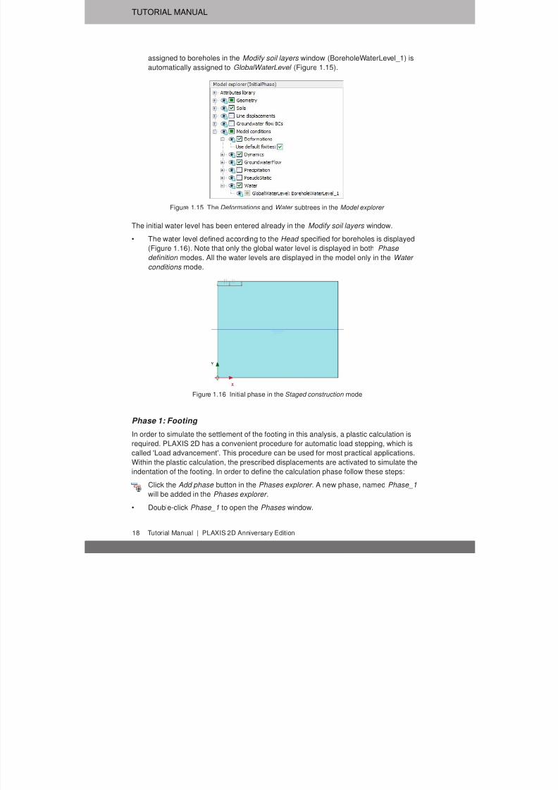
• Expand the Water subtree. The water level generated according to the Head value
PLAXIS 2D Anniversary Edition | Tutorial Manual 17
7/21/2019 2DAnniversaryEdition 1 Tutorial
http://slidepdf.com/reader/full/2danniversaryedition-1-tutorial 18/176
TUTORIAL MANUAL
assigned to boreholes in the Modify soil layers window (BoreholeWaterLevel_1) is
automatically assigned to GlobalWaterLevel (Figure 1.15).
Figure 1.15 The Deformations and Water subtrees in the Model explorer
The initial water level has been entered already in the Modify soil layers window.
• The water level defined according to the Head specified for boreholes is displayed
(Figure 1.16). Note that only the global water level is displayed in both Phase
definition modes. All the water levels are displayed in the model only in the Water
conditions mode.
Figure 1.16 Initial phase in the Staged construction mode
Phase 1: Footing
In order to simulate the settlement of the footing in this analysis, a plastic calculation is
required. PLAXIS 2D has a convenient procedure for automatic load stepping, which is
called 'Load advancement'. This procedure can be used for most practical applications.
Within the plastic calculation, the prescribed displacements are activated to simulate the
indentation of the footing. In order to define the calculation phase follow these steps:
Click the Add phase button in the Phases explorer . A new phase, named Phase_1will be added in the Phases explorer .
• Double-click Phase_1 to open the Phases window.
18 Tutorial Manual | PLAXIS 2D Anniversary Edition

7/21/2019 2DAnniversaryEdition 1 Tutorial
http://slidepdf.com/reader/full/2danniversaryedition-1-tutorial 19/176
SETTLEMENT OF A CIRCULAR FOOTING ON SAND
• In the ID box of the General subtree, write (optionally) an appropriate name for the
new phase (for example "Indentation").
• The current phase starts from the Initial phase , which contains the initial stress
state. The default options and values assigned are valid for this phase (Figure 1.17).
Figure 1.17 The Phases window for the Indentation phase
• Click OK to close the Phases window.
• Click the Staged construction tab to enter the corresponding mode.
• Right-click the prescribed displacement in the draw area and select the Activate
option in the appearing menu (Figure 1.18).
Figure 1.18 Activation of the prescribed displacement in the Staged construction mode
Hint: Calculation phases may be added, inserted or deleted using the Add , Insert
and Delete buttons in the Phases explorer or in the Phases window.
PLAXIS 2D Anniversary Edition | Tutorial Manual 19

7/21/2019 2DAnniversaryEdition 1 Tutorial
http://slidepdf.com/reader/full/2danniversaryedition-1-tutorial 20/176
TUTORIAL MANUAL
Execution of calculation
All calculation phases (two phases in this case) are marked for calculation (indicated by a
blue arrow). The execution order is controlled by the Start from phase parameter.
Click the Calculate button to start the calculation process. Ignore the warning thatno nodes and stress points have been selected for curves. During the execution of a
calculation, a window appears which gives information about the progress of the
actual calculation phase (Figure 1.19).
Figure 1.19 Active task window displaying the calculation progress
The information, which is continuously updated, shows the calculation progress, the
current step number, the global error in the current iteration and the number of plastic
points in the current calculation step. It will take a few seconds to perform the calculation.
When a calculation ends, the window is closed and focus is returned to the main window.
The phase list in the Phases explorer is updated. A successfully calculated phase is
indicated by a check mark inside a green circle.
Save the project before viewing results.
Viewing calculation results
Once the calculation has been completed, the results can be displayed in the Output
program. In the Output program, the displacement and stresses in the full two
dimensional model as well as in cross sections or structural elements can be viewed.
The computational results are also available in tabular form.
To check the applied load that results from the prescribed displacement of 0.05 m:
• Open the Phases window.
• For the current application the value of Force-Y in the Reached values subtree is
important. This value represents the total reaction force corresponding to the
applied prescribed vertical displacement, which corresponds to the total force under
20 Tutorial Manual | PLAXIS 2D Anniversary Edition

7/21/2019 2DAnniversaryEdition 1 Tutorial
http://slidepdf.com/reader/full/2danniversaryedition-1-tutorial 21/176
SETTLEMENT OF A CIRCULAR FOOTING ON SAND
1.0 radian of the footing (note that the analysis is axisymmetric). In order to obtain
the total footing force, the value of Force-Y should be multiplied by 2π (this gives a
value of about 588 kN).
The results can be evaluated in the Output program. In the Output window you can view
the displacements and stresses in the full geometry as well as in cross sections and instructural elements, if applicable. The computational results are also available in
tabulated form. To view the results of the footing analysis, follow these steps:
• Select the last calculation phase in the Phases explorer.
Click the View calculation results button in the side toolbar. As a result, the Output
program is started, showing the deformed mesh at the end of the selected
calculation phase (Figure 1.20). The deformed mesh is scaled to ensure that the
deformations are visible.
Figure 1.20 Deformed mesh
• In the Deformations menu select the Total displacements → |
u |
option. The plot
shows colour shadings of the total displacements. The colour distribution is
displayed in the legend at the right hand side of the plot.
Hint: The legend can be toggled on and off by clicking the corresponding option in
the View menu.
The total displacement distribution can be displayed in contours by clicking the
corresponding button in the toolbar. The plot shows contour lines of the total
displacements, which are labelled. An index is presented with the displacementvalues corresponding to the labels.
Clicking the Arrows button, the plot shows the total displacements of all nodes as
PLAXIS 2D Anniversary Edition | Tutorial Manual 21

7/21/2019 2DAnniversaryEdition 1 Tutorial
http://slidepdf.com/reader/full/2danniversaryedition-1-tutorial 22/176
TUTORIAL MANUAL
arrows, with an indication of their relative magnitude.
Hint: In addition to the total displacements, the Deformations menu allows for the
presentation of Incremental displacements . The incremental displacementsare the displacements that occurred within one calculation step (in this case
the final step). Incremental displacements may be helpful in visualising an
eventual failure mechanism.
» The plots of stresses and displacements may be combined with geometrical
features, as available in the Geometry menu.
• In the Stresses menu point to the Principal effective stresses and select the
Effective principal stresses option from the appearing menu. The plot shows the
effective principal stresses at the stress points of each soil element with an
indication of their direction and their relative magnitude (Figure 1.21).
Figure 1.21 Effective principal stresses
Click the Table button on the toolbar. A new window is opened in which a table is
presented, showing the values of the principal stresses and other stress measures
in each stress point of all elements.
1.3 CASE B: FLEXIBLE FOOTING
The project is now modified so that the footing is modelled as a flexible plate. This
enables the calculation of structural forces in the footing. The geometry used in this
exercise is the same as the previous one, except that additional elements are used to
model the footing. The calculation itself is based on the application of load rather than
prescribed displacement. It is not necessary to create a new model; you can start from
the previous model, modify it and store it under a different name. To perform this, follow
these steps:
22 Tutorial Manual | PLAXIS 2D Anniversary Edition

7/21/2019 2DAnniversaryEdition 1 Tutorial
http://slidepdf.com/reader/full/2danniversaryedition-1-tutorial 23/176
SETTLEMENT OF A CIRCULAR FOOTING ON SAND
Modifying the geometry
• In the Input program select the Save project as option of the File menu. Enter a
non-existing name for the current project file and click the Save button.
• Go back to the Structures mode.Right-click the prescribed displacement. In the right mouse button menu point to the
Line displacement option. In the expanded menu click on the Delete option (Figure
1.22).
Figure 1.22 Delete Prescribed displacement
• In the model right-click the line at the location of the footing. Point on Create and
select the Plate option in the appearing menu (Figure 1.23). A plate is created which
simulates the flexible footing.
Figure 1.23 Assignment of Plate to line
• In the model right-click again the line at the location of the footing. Point on Create and select the Line load option in the appearing menu (Figure 1.24).
PLAXIS 2D Anniversary Edition | Tutorial Manual 23

7/21/2019 2DAnniversaryEdition 1 Tutorial
http://slidepdf.com/reader/full/2danniversaryedition-1-tutorial 24/176
TUTORIAL MANUAL
Figure 1.24 Assignment of Line load to line
• In the Selection explorer the default input value of the distributed load is -1.0 kN/m2
in the y-direction. The input value will later be changed to the real value when the
load is activated.
Adding material properties for the footing
Click the Materials button in the side toolbar.
• Select Plates from the Set type drop-down menu in the Material sets window.
• Click the New button. A new window appears where the properties of the footing
can be entered.
• Write "Footing" in the Identification box. The Elastic option is selected by default for
the material type. Keep this option for this example.
• Enter the properties as listed in Table 1.2. Keep parameters that are not mentioned
in the table at their default values.
• Click OK . The new data set now appears in the tree view of the Material sets
window.
Hint: The equivalent thickness is automatically calculated by PLAXIS from thevalues of EA and EI . It cannot be defined manually.
Table 1.2 Material properties of the footing
Parameter Name Value Unit
Material type Type Elastic; Isotropic -
Normal stiffness EA 5 · 106 kN/m
Flexural rigidity EI 8.5 · 103 kNm2 /m
Weight w 0.0 kN/m/m
Poisson's ratio ν 0.0 -
• Drag the set "Footing" to the draw area and drop it on the footing. Note that the
shape of the cursor changes to indicate that it is valid to drop the material set.
24 Tutorial Manual | PLAXIS 2D Anniversary Edition

7/21/2019 2DAnniversaryEdition 1 Tutorial
http://slidepdf.com/reader/full/2danniversaryedition-1-tutorial 25/176
SETTLEMENT OF A CIRCULAR FOOTING ON SAND
Hint: If the Material sets window is displayed over the footing and hides it, click on
its header and drag it to another position.
• Close the database by clicking the OK button.
Generating the mesh
• Proceed to the Mesh mode.
Create the mesh. Use the default option for the Element distribution parameter
(Medium ).
View the mesh.
• Click on the Close tab to close the Output program.
Hint: Regeneration of the mesh results in a redistribution of nodes and stress
points.
Calculations
• Proceed to the Staged construction mode.
• The initial phase is the same as in the previous case.
• Double-click the following phase (Phase_1) and enter an appropriate name for the
phase ID. Keep Plastic as Calculation type and keep Staged construction as loading
type.
• Close the Phases window.
• In the Staged construction mode activate the load and plate. The model is shown in
Figure 1.25.
Figure 1.25 Active plate and load in the model
PLAXIS 2D Anniversary Edition | Tutorial Manual 25

7/21/2019 2DAnniversaryEdition 1 Tutorial
http://slidepdf.com/reader/full/2danniversaryedition-1-tutorial 26/176
TUTORIAL MANUAL
• In the Selection explorer assign −188 kN/m2 to the vertical component of the line
load (Figure 1.26). Note that this gives a total load that is approximately equal to the
footing force that was obtained from the first part of this tutorial. (188 kN/m2 · π·(1.0
m)2 ≈ 590 kN).
Figure 1.26 Definition of the load components in the Selection explorer
• No changes are required in the Water conditions tabsheet.
The calculation definition is now complete. Before starting the calculation it is advisable
to select nodes or stress points for a later generation of load-displacement curves or
stress and strain diagrams. To do this, follow these steps:
Click the Select points for curves button in the side toolbar. As a result, all the nodes
and stress points are displayed in the model in the Output program. The points can
be selected either by directly clicking on them or by using the options available in the
Select points window.
• In the Select points window enter (0.0 4.0) for the coordinates of the point of interest
and click Search closest . The nodes and stress points located near that specific
location are listed.
• Select the node at exactly (0.0 4.0) by checking the box in front of it. The selected
node is indicated by ’A’ in the model when the Selection labels option is selected in
the Mesh menu.
Hint: Instead of selecting nodes or stress points for curves before starting the
calculation, points can also be selected after the calculation when viewing
the output results. However, the curves will be less accurate since only the
results of the saved calculation steps will be considered.
To select the desired nodes by clicking on them, it may be convenient to use
the Zoom in option on the toolbar to zoom into the area of interest.
• Click the Update button to return to the Input program.
• Check if both calculation phases are marked for calculation by a blue arrow. If this is
not the case click the symbol of the calculation phase or right-click and select Mark
26 Tutorial Manual | PLAXIS 2D Anniversary Edition

7/21/2019 2DAnniversaryEdition 1 Tutorial
http://slidepdf.com/reader/full/2danniversaryedition-1-tutorial 27/176
SETTLEMENT OF A CIRCULAR FOOTING ON SAND
for calculation from the pop-up menu.
Click the Calculate button to start the calculation.
Save the project after the calculation has finished.
Viewing the results
After the calculation the results of the final calculation step can be viewed by clicking
the View calculation results button. Select the plots that are of interest. The
displacements and stresses should be similar to those obtained from the first part of
the exercise.
Click the Select structures button in the side toolbar and double click the footing. A
new window opens in which either the displacements or the bending moments of the
footing may be plotted (depending on the type of plot in the first window).
• Note that the menu has changed. Select the various options from the Forces menuto view the forces in the footing.
Hint: Multiple (sub-)windows may be opened at the same time in the Output
program. All windows appear in the list of the Window menu. PLAXIS follows
the Windows standard for the presentation of sub-windows (Cascade , Tile ,
Minimize , Maximize , etc).
Generating a load-displacement curve In addition to the results of the final calculation step it is often useful to view a
load-displacement curve. In order to generate the load-displacement curve as given in
Figure 1.28, follow these steps:
Click the Curves manager button in the toolbar. The Curves manager window pops
up.
Figure 1.27 Curve generation window
PLAXIS 2D Anniversary Edition | Tutorial Manual 27

7/21/2019 2DAnniversaryEdition 1 Tutorial
http://slidepdf.com/reader/full/2danniversaryedition-1-tutorial 28/176
TUTORIAL MANUAL
• In the Charts tabsheet, click New . The Curve generation window pops up (Figure
1.27).
• For the x −axis, select point A (0.00 / 4.00) from the drop-down menu. Select the |u |option for the Total displacements option of the Deformations .
• For the y −axis, select the Project option from the drop-down menu. Select the
ΣMstage option of the Multipliers . ΣMstage is the proportion of the specified
changes that has been applied. Hence the value will range from 0 to 1, which
means that 100% of the prescribed load has been applied and the prescribed
ultimate state has been fully reached.
Hint: To re-enter the Settings window (in the case of a mistake, a desired
regeneration or modification) you can double click the chart in the legend at
the right of the chart. Alternatively, you may open the Settings window by
selecting the corresponding option from the Format menu.» The properties of the chart can be modified in the Chart tabsheet whereas
the properties curve can be modified in the corresponding tabsheet.
• Click OK to accept the input and generate the load-displacement curve. As a result
the curve of Figure 1.28 is plotted.
Figure 1.28 Load-displacement curve for the footing
28 Tutorial Manual | PLAXIS 2D Anniversary Edition

7/21/2019 2DAnniversaryEdition 1 Tutorial
http://slidepdf.com/reader/full/2danniversaryedition-1-tutorial 29/176
SUBMERGED CONSTRUCTION OF AN EXCAVATION
2 SUBMERGED CONSTRUCTION OF AN EXCAVATION
This tutorial illustrates the use of PLAXIS for the analysis of submerged construction of
an excavation. Most of the program features that were used in Tutorial 1 will be utilised
here again. In addition, some new features will be used, such as the use of interfacesand anchor elements, the generation of water pressures and the use of multiple
calculation phases. The new features will be described in full detail, whereas the features
that were treated in Tutorial 1 will be described in less detail. Therefore it is suggested
that Tutorial 1 should be completed before attempting this exercise.
This tutorial concerns the construction of an excavation close to a river. The submerged
excavation is carried out in order to construct a tunnel by the installation of prefabricated
tunnel segments which are 'floated' into the excavation and 'sunk' onto the excavation
bottom. The excavation is 30 m wide and the final depth is 20 m. It extends in longitudinal
direction for a large distance, so that a plane strain model is applicable. The sides of the
excavation are supported by 30 m long diaphragm walls, which are braced by horizontalstruts at an interval of 5 m. Along the excavation a surface load is taken into account.
The load is applied from 2 m from the diaphragm wall up to 7 m from the wall and has a
magnitude of 5 kN/m2 /m (Figure 2.1).
The upper 20 m of the subsoil consists of soft soil layers, which are modelled as a single
homogeneous clay layer. Underneath this clay layer there is a stiffer sand layer, which
extends to a large depth. 30 m of the sand layer are considered in the model.
x
y
43 m43 m 5 m5 m 2 m2 m 30 m
1 m
19 m
10 m
20 m
ClayClay
Sand
Diaphragm wall
to be excavated
Strut
5 kN/m2 /m5 kN/m2 /m
Figure 2.1 Geometry model of the situation of a submerged excavation
Since the geometry is symmetric, only one half (the left side) is considered in the
analysis. The excavation process is simulated in three separate excavation stages. The
diaphragm wall is modelled by means of a plate, such as used for the footing in the
previous tutorial. The interaction between the wall and the soil is modelled at both sides
by means of interfaces. The interfaces allow for the specification of a reduced wall friction
compared to the friction in the soil. The strut is modelled as a spring element for which
the normal stiffness is a required input parameter.
PLAXIS 2D Anniversary Edition | Tutorial Manual 29
7/21/2019 2DAnniversaryEdition 1 Tutorial
http://slidepdf.com/reader/full/2danniversaryedition-1-tutorial 30/176
TUTORIAL MANUAL
Objectives:
• Modelling soil-structure interaction using the Interface feature.
• Advanced soil models (Soft Soil model and Hardening Soil model ).
• Undrained (A) drainage type.
• Defining Fixed-end-anchor .
• Creating and assigning material data sets for anchors.
• Simulation of excavation (cluster de-activation).
2.1 INPUT
To create the geometry model, follow these steps:
General settings
• Start the Input program and select Start a new project from the Quick select dialog
box.
• In the Project tabsheet of the Project properties window, enter an appropriate title.
• In the Model tabsheet keep the default options for Model (Plane strain ), and
Elements (15-Node ).
• Keep the default values for units and the general parameters.
• Set the model dimensions to x min = 0.0 m, x max = 65.0 m, y min = -30.0 m, y max =
20.0 m and press OK to close the Project properties window.
Definition of soil stratigraphy
To define the soil stratigraphy:
Create a borehole at x = 0. The Modify soil layers window pops up.
• Add the top soil layer and specify its height by setting the top level to 20 m and the
bottom level to 0 m.
• Add the bottom soil layer and specify its height by keeping the top level at 0 m and
by setting the bottom level to -30 m.
• Set the Head in the borehole to 18.0 m.
Two data sets need to be created; one for the clay layer and one for the sand layer. To
create the material data sets, follow these steps:
Click the Materials button in the Modify soil layers window. The Material sets window
pops up where the Soil and interfaces option is selected by default as the Set type .
• Click the New button in the Material sets window to create a new data set.
• For the clay layer, enter "Clay" for the Identification and select Soft soil as the
Material model . Set the Drainage type to Undrained (A).
• Enter the properties of the clay layer, as listed in Table 2.1, in the General ,
Parameters and Flow parameters tabsheets.
30 Tutorial Manual | PLAXIS 2D Anniversary Edition

7/21/2019 2DAnniversaryEdition 1 Tutorial
http://slidepdf.com/reader/full/2danniversaryedition-1-tutorial 31/176
SUBMERGED CONSTRUCTION OF AN EXCAVATION
Table 2.1 Material properties of the sand and clay layer and the interfaces
Parameter Name Clay Sand Unit
General
Material model Model Soft soil Hardening soil -
Type of material behaviour Type Undrained (A) Drained -Soil unit weight above phreatic level γ unsat 16 17 kN/m3
Soil unit weight below phreatic level γ sat 18 20 kN/m3
Initial void ratio e init 1.0 0.5 -
Parameters
Modified compression index λ∗ 3.0· 10-2 - -
Modified swelling index κ∗ 8.5· 10-3 - -
Secant stiffness in standard drained triaxial test E ref 50 - 4.0· 104 kN/m2
Tangent stiffness for primary oedometer loading E ref oed - 4.0· 104 kN/m2
Unloading / reloading stiffness E ref ur - 1.2· 105 kN/m2
Power for stress-level dependency of stiffness m - 0.5 -
Cohesion (constant) c ref ' 1.0 0.0 kN/m2
Friction angle ϕ' 25 32
◦
Dilatancy angle ψ 0.0 2.0 ◦
Poisson's ratio ν ur ' 0.15 0.2 -
K 0-value for normal consolidation K nc 0 0.5774 0.4701 -
Flow parameters
Permeability in horizontal direction k x 0.001 1.0 m/day
Permeability in vertical direction k y 0.001 1.0 m/day
Interfaces
Interface strength − Manual Manual -
Strength reduction factor inter. R inter 0.5 0.67 -
Initial
K 0 determination − Automatic Automatic -
Over-consolidation ratio OCR 1.0 1.0 -Pre-overburden pressure POP 5.0 0.0 kN/m2
• Click the Interfaces tab. Select the Manual option in the Strength drop-down menu.
Enter a value of 0.5 for the parameter R inter . This parameter relates the strength of
the soil to the strength in the interfaces, according to the equations:
tanϕinterface = R inter tan ϕsoil and c inter = R inter c soil
where:
c soil = c ref (see Table 2.1)
Hence, using the entered R inter -value gives a reduced interface friction (wallfrictions) and interface cohesion (adhesion) compared to the friction angle and the
cohesion in the adjacent soil.
• In the Initial tabsheet keep the default option for the K 0 determination and the
default value for the overconsolidation ratio (OCR ). Set the pre-overburden pressure
(POP ) value to 5.0.
• For the sand layer, enter "Sand" for the Identification and select Hardening soil as
the Material model . The material type should be set to Drained .
• Enter the properties of the sand layer, as listed in Table 2.1, in the corresponding
edit boxes of the General and Parameters tabsheet.• Click the Interfaces tab. In the Strength box, select the Manual option. Enter a value
of 0.67 for the parameter R inter . Close the data set.
PLAXIS 2D Anniversary Edition | Tutorial Manual 31
7/21/2019 2DAnniversaryEdition 1 Tutorial
http://slidepdf.com/reader/full/2danniversaryedition-1-tutorial 32/176
TUTORIAL MANUAL
• Assign the material datasets to the corresponding soil layers.
Hint: When the Rigid option is selected in the Strength drop-down, the interface
has the same strength properties as the soil (R inter = 1.0).» Note that a value of R inter < 1.0, reduces the strength as well as the the
stiffness of the interface (Section ?? of the Reference Manual).
» Instead of accepting the default data sets of interfaces, data sets can directly
be assigned to interfaces by selecting the proper data set in the Material
mode drop-down menu in the Object explorers .
2.1.1 DEFINITION OF STRUCTURAL ELEMENTS
The creation of diaphragm walls, strut, surface load and excavation levels is describedbelow.
• Click the Structures tab to proceed with the input of structural elements in the
Structures mode.
To define the diaphragm wall:
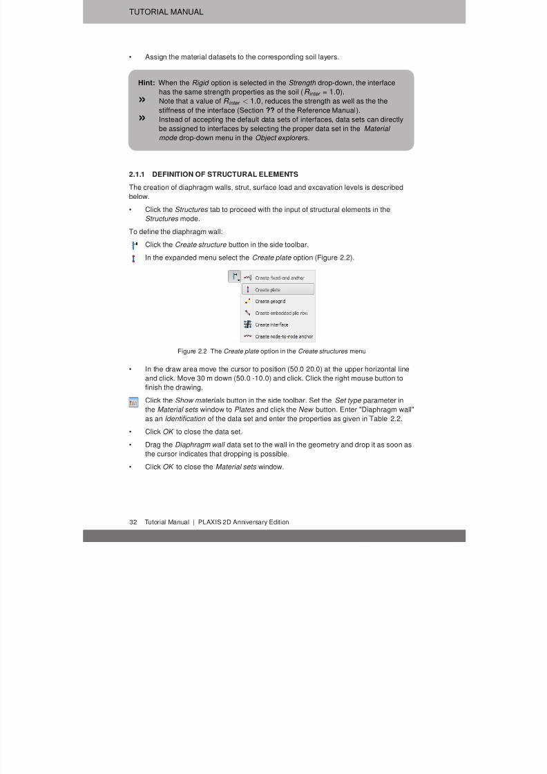
Click the Create structure button in the side toolbar.
In the expanded menu select the Create plate option (Figure 2.2).
Figure 2.2 The Create plate option in the Create structures menu
• In the draw area move the cursor to position (50.0 20.0) at the upper horizontal line
and click. Move 30 m down (50.0 -10.0) and click. Click the right mouse button tofinish the drawing.
Click the Show materials button in the side toolbar. Set the Set type parameter in
the Material sets window to Plates and click the New button. Enter "Diaphragm wall"
as an Identification of the data set and enter the properties as given in Table 2.2.
• Click OK to close the data set.
• Drag the Diaphragm wall data set to the wall in the geometry and drop it as soon as
the cursor indicates that dropping is possible.
• Click OK to close the Material sets window.
32 Tutorial Manual | PLAXIS 2D Anniversary Edition

7/21/2019 2DAnniversaryEdition 1 Tutorial
http://slidepdf.com/reader/full/2danniversaryedition-1-tutorial 33/176
SUBMERGED CONSTRUCTION OF AN EXCAVATION
Table 2.2 Material properties of the diaphragm wall (Plate)
Parameter Name Value Unit
Type of behaviour Material type Elastic; Isotropic
Normal stiffness EA 7.5 · 106 kN/m
Flexural rigidity EI 1.0 · 106 kNm2 /m
Unit weight w 10.0 kN/m/m
Poisson's ratio ν 0.0 -
Hint: In general, only one point can exist at a certain coordinate and only one line
can exist between two points. Coinciding points or lines will automatically be
reduced to single points or lines. More information is available in Section ??
of the Reference Manual.
To define interfaces:• Right-click the plate representing the diaphragm wall. Point to Create and click on
the Positive interface option in the appearing menu (Figure 2.3). In the same way
assign a negative interface as well.
Figure 2.3 Positive interface assignment to existing geometry
Hint: In order to identify interfaces at either side of a geometry line, a positive sign
(⊕) or negative sign (⊖) is added. This sign has no physical relevance or
influence on the results.
» A Virtual thickness factor can be defined for interfaces. This is a purely
numerical value, which can be used to optimise the numerical performance
of the interface. To define it, select the interface in the draw area and specify
the value to the Virtual thickness factor parameter in the Selection explorer .
Non-experienced users are advised not to change the default value. Formore information about interface properties see the Reference Manual.
PLAXIS 2D Anniversary Edition | Tutorial Manual 33

7/21/2019 2DAnniversaryEdition 1 Tutorial
http://slidepdf.com/reader/full/2danniversaryedition-1-tutorial 34/176
TUTORIAL MANUAL
To define the excavation levels:
Click the Create line button in the side toolbar.
• To define the first excavation stage move the cursor to position (50.0 18.0) at the
wall and click. Move the cursor 15 m to the right (65.0 18.0) and click again. Clickthe right mouse button to finish drawing the first excavation stage.
• To define the second excavation stage move the cursor to position (50.0 10.0) and
click. Move to (65.0 10.0) and click again. Click the right mouse button to finish
drawing the second excavation stage.
• The third excavation stage is automatically defined as it corresponds to the
boundary between the soil layers (y = 0.0).
To define the strut:
Click the Create structure button in the side toolbar and select the Create fixed-end
anchor button in the expanded menu.
• Move the cursor to (50.0 19.0) and click the left mouse button. A fixed-end anchor is
is added, being represented by a rotated T with a fixed size.
Click the Show materials button in the side toolbar. Set the Set type parameter in
the Material sets window to Anchor and click the New button. Enter "Strut" as an
Identification of the data set and enter the properties as given in Table 2.3. Click OK
to close the data set.
• Click OK to close the Material sets window.
Table 2.3 Material properties of the strut (anchor)
Parameter Name Value Unit
Type of behaviour Material type Elastic -
Normal stiffness EA 2·106 kN
Spacing out of plane Lspacing 5.0 m
• Make sure that the fixed-end anchor is selected in the draw area.
• In the Selection explorer assign the material data set to the strut by selecting the
corresponding option in the Material drop-down menu.
• The anchor is oriented in the model according to the Direction x and Direction y
parameters in the Selection explorer . The default orientation is valid in this tutorial.
• Enter an Equivalent length of 15 m corresponding to half the width of the excavation
(Figure 2.4).
Hint: The Equivalent length is the distance between the connection point and the
position in the direction of the anchor rod where the displacement is zero.
To define the distributed load:
Click the Create load button in the side toolbar
Select the Create line load option in the expanded menu to define a distributed load
(Figure 2.5).
34 Tutorial Manual | PLAXIS 2D Anniversary Edition
7/21/2019 2DAnniversaryEdition 1 Tutorial
http://slidepdf.com/reader/full/2danniversaryedition-1-tutorial 35/176
SUBMERGED CONSTRUCTION OF AN EXCAVATION
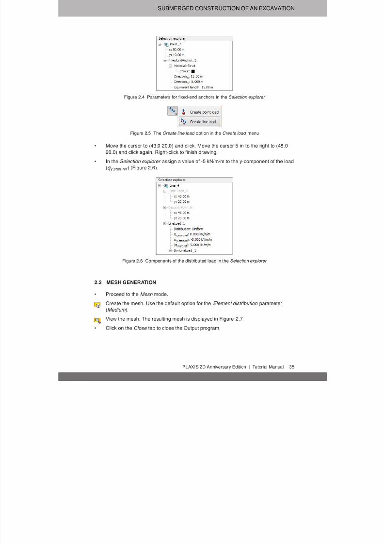
Figure 2.4 Parameters for fixed-end anchors in the Selection explorer
Figure 2.5 The Create line load option in the Create load menu
• Move the cursor to (43.0 20.0) and click. Move the cursor 5 m to the right to (48.0
20.0) and click again. Right-click to finish drawing.
• In the Selection explorer assign a value of -5 kN/m/m to the y-component of the load
(q y ,start ,ref ) (Figure 2.6).
Figure 2.6 Components of the distributed load in the Selection explorer
2.2 MESH GENERATION
• Proceed to the Mesh mode.
Create the mesh. Use the default option for the Element distribution parameter
(Medium ).
View the mesh. The resulting mesh is displayed in Figure 2.7.
• Click on the Close tab to close the Output program.
PLAXIS 2D Anniversary Edition | Tutorial Manual 35

7/21/2019 2DAnniversaryEdition 1 Tutorial
http://slidepdf.com/reader/full/2danniversaryedition-1-tutorial 36/176
TUTORIAL MANUAL
Figure 2.7 The generated mesh
2.3 CALCULATIONS
In practice, the construction of an excavation is a process that can consist of several
phases. First, the wall is installed to the desired depth. Then some excavation is carried
out to create space to install an anchor or a strut. Then the soil is gradually removed to
the final depth of the excavation. Special measures are usually taken to keep the water
out of the excavation. Props may also be provided to support the retaining wall.
In PLAXIS, these processes can be simulated with the Staged construction loading type
available in the General subtree of the Phases window. It enables the activation or
deactivation of weight, stiffness and strength of selected components of the finite elementmodel. Note that modifications in the Staged construction mode of the program are
possible only for this type of loading. The current tutorial explains the use of this powerful
calculation option for the simulation of excavations.
• Click on the Staged construction tab to proceed with the definition of the calculation
phases.
• The initial phase has already been introduced. Keep its calculation type as K0
procedure . Make sure all the soil volumes are active and all the structural elements
and load are inactive.
Phase 1: External load
In the Phases explorer click the Add phase button to introduce a new phase.
• The default settings are valid for this phase. In the model the full geometry is active
except for the wall, interfaces, strut and load.
Click the Select multiple objects button in the side toolbar. In the appearing menu
point to Select line and click on the Select plates option (Figure 2.8).
• In the draw area define a rectangle including all the plate elements (Figure 2.9).
• Right-click the wall in the draw area and select the Activate option from the
appearing menu. The wall is now visible in the color that is specified in the materialdataset.
36 Tutorial Manual | PLAXIS 2D Anniversary Edition

7/21/2019 2DAnniversaryEdition 1 Tutorial
http://slidepdf.com/reader/full/2danniversaryedition-1-tutorial 37/176
SUBMERGED CONSTRUCTION OF AN EXCAVATION
Figure 2.8 The Select plates option
Figure 2.9 Multi-selection of plates in the draw area
• Right-click the distributed load to activate it and select the Activate option from the
appearing menu. The load has been defined in the Structures mode as −5 kN/m/m.
The value can be checked in the Selection explorer .
• Make sure all the interfaces in the model are active.
Hint: The selection of an interface is done by right-clicking the corresponding
geometry line and subsequently selecting the corresponding interface
(positive or negative) from the appearing menu.
PLAXIS 2D Anniversary Edition | Tutorial Manual 37

7/21/2019 2DAnniversaryEdition 1 Tutorial
http://slidepdf.com/reader/full/2danniversaryedition-1-tutorial 38/176
TUTORIAL MANUAL
Phase 2: First excavation stage
In the Phases explorer click the Add phase button to introduce a new phase.
• A new calculation phase appears in the Phases explorer . Note that the program
automatically presumes that the current phase should start from the previous oneand that the same objects are active.
Hint: To copy the settings of the parent phase, select the phase in the Phases
explorer and then click the Add phase button. Note that the settings of the
parent phase are not copied when it is specified by selecting it in the Start
from phase drop-down menu in the Phases window.
• The default settings are valid for this phase. In the Staged construction mode all the
structure elements except the fixed-end anchor are active.
• In the draw area right-click the top right cluster and select the Deactivate option in
the appearing menu. Figure 2.10 displays the model for the first excavation phase.
Figure 2.10 Model view for the first excavation phase
Phase 3: Installation of strut
Add a new phase.
• Activate the strut. The strut should turn black to indicate it is active.
Phase 4: Second (submerged) excavation stage
Add a new phase.
• Deactivate the second cluster from the top on the right side of the mesh. It should
be the topmost active cluster (Figure 2.11).
38 Tutorial Manual | PLAXIS 2D Anniversary Edition

7/21/2019 2DAnniversaryEdition 1 Tutorial
http://slidepdf.com/reader/full/2danniversaryedition-1-tutorial 39/176
SUBMERGED CONSTRUCTION OF AN EXCAVATION
Figure 2.11 Model view for the second excavation phase
Hint: Note that in PLAXIS the pore pressures are not automatically deactivated
when deactivating a soil cluster. Hence, in this case, the water remains in the
excavated area and a submerged excavation is simulated.
Phase 5: Third excavation stage
Add a new phase.
• In the final calculation stage the excavation of the last clay layer inside the pit is
simulated. Deactivate the third cluster from the top on the right hand side of the
mesh (Figure 2.12).
Figure 2.12 Model view for the third excavation phase
The calculation definition is now complete. Before starting the calculation it is suggested
that you select nodes or stress points for a later generation of load-displacement curves
or stress and strain diagrams. To do this, follow the steps given below.
Click the Select points for curves button in the side toolbar. The connectivity plot is
displayed in the Output program and the Select points window is activated.
• Select some nodes on the wall at points where large deflections can be expected
PLAXIS 2D Anniversary Edition | Tutorial Manual 39
7/21/2019 2DAnniversaryEdition 1 Tutorial
http://slidepdf.com/reader/full/2danniversaryedition-1-tutorial 40/176
TUTORIAL MANUAL
(e.g. 50.0 10.0). The nodes located near that specific location are listed. Select the
convenient one by checking the box in front of it in the list. Close the Select points
window.
• Click on the Update tab to close the Output program and go back to the Input
program.
Calculate the project.
During a Staged construction calculation phase, a multiplier called ΣMstage is increased
from 0.0 to 1.0. This parameter is displayed on the calculation info window. As soon as
ΣMstage has reached the value 1.0, the construction stage is completed and the
calculation phase is finished. If a Staged construction calculation finishes while ΣMstage is smaller than 1.0, the program will give a warning message. The most likely reason for
not finishing a construction stage is that a failure mechanism has occurred, but there can
be other causes as well. See the Reference Manual for more information about Staged
construction .
2.4 RESULTS
In addition to the displacements and the stresses in the soil, the Output program can be
used to view the forces in structural objects. To examine the results of this project, follow
these steps:
• Click the final calculation phase in the Calculations window.
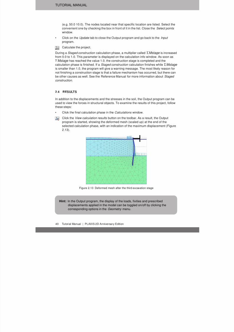
Click the View calculation results button on the toolbar. As a result, the Output
program is started, showing the deformed mesh (scaled up) at the end of theselected calculation phase, with an indication of the maximum displacement (Figure
2.13).
Figure 2.13 Deformed mesh after the third excavation stage
Hint: In the Output program, the display of the loads, fixities and prescribed
displacements applied in the model can be toggled on/off by clicking thecorresponding options in the Geometry menu.
40 Tutorial Manual | PLAXIS 2D Anniversary Edition

7/21/2019 2DAnniversaryEdition 1 Tutorial
http://slidepdf.com/reader/full/2danniversaryedition-1-tutorial 41/176
SUBMERGED CONSTRUCTION OF AN EXCAVATION
• Select |∆u | from the side menu displayed as the mouse pointer is located on the
Incremental displacements option of the Deformations menu. The plot shows colour
shadings of the displacement increments, which indicates the forming of a
'mechanism' of soil movement behind the wall.
Click the Arrows button in the toolbar. The plot shows the displacement incrementsof all nodes as arrows. The length of the arrows indicates the relative magnitude.
• In the Stresses menu point to the Principal effective stresses and select the
Effective principal stresses option from the appearing menu. The plot shows the
effective principal stresses at the three middle stress points of each soil element
with an indication of their direction and their relative magnitude. Note that the
Central principal stresses button is selected in the toolbar. The orientation of the
principal stresses indicates a large passive zone under the bottom of the excavation
and a small passive zone behind the strut (Figure 2.14).
Figure 2.14 Principal stresses after excavation
To plot the shear forces and bending moments in the wall follow the steps given below.
• Double-click the wall. A new window is opened showing the axial force.
• Select the bending moment M from the Forces menu. The bending moment in the
wall is displayed with an indication of the maximum moment (Figure 2.15).
Figure 2.15 Bending moments in the wall
PLAXIS 2D Anniversary Edition | Tutorial Manual 41

7/21/2019 2DAnniversaryEdition 1 Tutorial
http://slidepdf.com/reader/full/2danniversaryedition-1-tutorial 42/176
TUTORIAL MANUAL
• Select Shear forces Q from the Forces menu. The plot now shows the shear forces
in the wall.
Hint: The Window menu may be used to switch between the window with the
forces in the wall and the stresses in the full geometry. This menu may also
be used to Tile or Cascade the two windows, which is a common option in a
Windows environment.
• Select the first window (showing the effective stresses in the full geometry) from the
Window menu. Double-click the strut. The strut force (in kN) is shown in the
displayed table.
• Click the Curves manager button on the toolbar. As a result, the Curves manager
window will pop up.
• Click New to create a new chart. The Curve generation window pops up.
• For the x-axis select the point A from the drop-down menu. In the tree select
Deformations - Total displacements - |u| .
• For the y-axis keep the Project option in the drop-down menu. In the tree select
Multiplier - ΣMstage .
• Click OK to accept the input and generate the load-displacement curve. As a result
the curve of Figure 2.16 is plotted.
Figure 2.16 Load-displacement curve of deflection of wall
The curve shows the construction stages. For each stage, the parameter ΣMstage
changes from 0.0 to 1.0. The decreasing slope of the curve in the last stage indicates
that the amount of plastic deformation is increasing. The results of the calculation
indicate, however, that the excavation remains stable at the end of construction.
42 Tutorial Manual | PLAXIS 2D Anniversary Edition

7/21/2019 2DAnniversaryEdition 1 Tutorial
http://slidepdf.com/reader/full/2danniversaryedition-1-tutorial 43/176
DRY EXCAVATION USING A TIE BACK WALL
3 DRY EXCAVATION USING A TIE BACK WALL
This example involves the dry construction of an excavation. The excavation is supported
by concrete diaphragm walls. The walls are tied back by prestressed ground anchors.
10 m 2 m 20 m
5 m
Silt
Sand
Loam
ground anchor
Final excavation level
3 m
3 m
4 m
10 kN/m2
Figure 3.1 Excavation supported by tie back walls
PLAXIS allows for a detailed modelling of this type of problem. It is demonstrated in this
example how ground anchors are modelled and how prestressing is applied to the
anchors. Moreover, the dry excavation involves a groundwater flow calculation to
generate the new water pressure distribution. This aspect of the analysis is explained in
detail.
Objectives:
• Modelling ground anchors.
• Generating pore pressures by groundwater flow.
• Displaying the contact stresses and resulting forces in the model (Forces view).
• Scaling the displayed results.
3.1 INPUT
The excavation is 20 m wide and 10 m deep. 16 m long concrete diaphragm walls of 0.35
m thickness are used to retain the surrounding soil. Two rows of ground anchors are
used at each wall to support the walls. The anchors have a total length of 14.5 m and aninclination of 33.7◦ (2:3). On the left side of the excavation a surface load of 10 kN/m2 is
taken into account.
The relevant part of the soil consists of three distinct layers. From the ground surface to a
depth of 3 m there is a fill of relatively loose fine sandy soil. Underneath the fill, down to a
minimum depth of 15 m, there is a more or less homogeneous layer consisting of dense
well-graded sand. This layer is particular suitable for the installation of the ground
anchors. The underlying layer consists of loam and lies to a large depth. 15 m of this
layer is considered in the model. In the initial situation there is a horizontal phreatic level
at 3 m below the ground surface (i.e. at the base of the fill layer).
PLAXIS 2D Anniversary Edition | Tutorial Manual 43

7/21/2019 2DAnniversaryEdition 1 Tutorial
http://slidepdf.com/reader/full/2danniversaryedition-1-tutorial 44/176
TUTORIAL MANUAL
General settings
• Start the Input program and select Start a new project from the Quick select dialog
box.
• In the Project tabsheet of the Project properties window, enter an appropriate title.• In the Model tabsheet keep the default options for Model (Plane strain ), and
Elements (15-Node ).
• Keep the default values for units and the general parameters.
• Set the model dimensions to x min = 0.0 m, x max = 100.0 m, y min = 0.0 m, y max = 30.0
m and press OK to close the Project properties window.
Definition of soil stratigraphy
To define the soil stratigraphy:
Create a borehole at x = 0. The Modify soil layers window pops up.
• Add three soil layers to the borehole. Locate the ground level at y = 30 m by
assigning 30 to the Top level of the uppermost layer. The bottom levels of the layers
are located at 27, 15 and 0 m, respectively.
• Set the Head to 23 m. The layer stratigraphy is shown in Figure 3.2.
Figure 3.2 The Modify soil layers window
Define three data sets for soil and interfaces with the parameters given in Table 3.1.
• Assign the material data sets to the corresponding soil layers (Figure 3.2).
44 Tutorial Manual | PLAXIS 2D Anniversary Edition

7/21/2019 2DAnniversaryEdition 1 Tutorial
http://slidepdf.com/reader/full/2danniversaryedition-1-tutorial 45/176
DRY EXCAVATION USING A TIE BACK WALL
Table 3.1 Soil and interface properties
Parameter Name Silt Sand Loam Unit
General
Material model Model Hardening soil Hardening soil Hardening soil -
Type of material behaviour Type Drained Drained Drained -Soil unit weight above phreatic level γ unsat 16 17 17 kN/m3
Soil unit weight below phreatic level γ sat 20 20 19 kN/m3
Parameters
Secant stiffness in standard drainedtriaxial test
E ref 50 2.0· 104 3.0· 104 1.2· 104 kN/m2
Tangent stiffness for primaryoedometer loading
E ref oed 2.0· 104 3.0· 104 8.0· 103 kN/m2
Unloading / reloading stiffness E ref ur 6.0· 104 9.0· 104 3.6· 104 kN/m2
Power for stress-level dependency ofstiffness
m 0.5 0.5 0.8 -
Cohesion c ref ' 1.0 0.0 5.0 kN/m2
Friction angle ϕ' 30 34 29 ◦
Dilatancy angle ψ 0.0 4.0 0.0 ◦
Poisson's ratio ν ur ' 0.2 0.2 0.2 -
K 0-value for normal consolidation K nc 0 0.5 0.4408 0.5152 -
Flow parameters
Data set - USDA USDA USDA -
Model - VanGenuchten
VanGenuchten
VanGenuchten
-
Soil type - Silt Sand Loam -
< 2µm - 6.0 4.0 20.0 %
2µm − 50µm - 87.0 4.0 40.0 %
50µm − 2mm - 7.0 92.0 40.0 %
Set parameters to defaults - Yes Yes Yes -
Permeability in horizontal direction k x 0.5996 7.128 0.2497 m/dayPermeability in vertical direction k y 0.5996 7.128 0.2497 m/day
Interfaces
Interface strength − Manual Manual Rigid -
Strength reduction factor inter. R inter 0.65 0.70 1.0 -
Consider gap closure − Yes Yes Yes -
Initial
K 0 determination − Automatic Automatic Automatic -
Over-consolidation ratio OCR 1.0 1.0 1.0 -
Pre-overburden pressure POP 0.0 0.0 25.0 kN/m2
3.1.1 DEFINITION OF STRUCTURAL ELEMENTS
In the Structures mode, model the diaphragm walls as plates passing through (40.0
30.0) - (40.0 14.0) and (60.0 30.0) - (60.0 14.0).
• Multi-select the plates in the model.
• In the Selection explorer click on Material . The view will change displaying a
drop-down menu and a plus button next to it (Figure 3.3).
Click the plus button. A new empty material set is created for plates.
• Define the material data set for the diaphragm walls according to the properties are
listed in Table 3.2. The concrete has a Young's modulus of 35 GN/m2 and the wall is
0.35 m thick.
PLAXIS 2D Anniversary Edition | Tutorial Manual 45

7/21/2019 2DAnniversaryEdition 1 Tutorial
http://slidepdf.com/reader/full/2danniversaryedition-1-tutorial 46/176
TUTORIAL MANUAL
Figure 3.3 Material assignment in the Selection explorer
Table 3.2 Properties of the diaphragm wall (plate)
Parameter Name Value Unit
Material type Type Elastic; Isotropic -
End bearing − Yes -
Normal stiffness EA 1.2 · 107 kN/m
Flexural rigidity EI 1.2 · 105 kNm2 /m
Weight w 8.3 kN/m/m
Poisson's ratio ν 0.15 -
• Assign positive and negative interfaces to the geometry lines created to represent
the diaphragm walls.
The soil is excavated in three stages. The first excavation layer corresponds to the bottom
of the silt layer and it is automatically created. To define the remaining excavation stages:
Define the second excavation phase by drawing a line through (40.0 23.0) and (60.0
23.0).
Define the third excavation phase by drawing a line through (40.0 20.0) and (60.0
20.0).
A ground anchor can be modelled by a combination of a node-to-node anchor and an
embedded pile. The embedded pile simulates the grouted part of the anchor whereas the
node-to-node anchor simulates the free length. In reality there is a complex
three-dimensional state of stress around the grout body which cannot be simulated in a
2D model.
Define the node-to-node anchors according to Table 3.3.
Table 3.3 Node to node anchor coordinates
Anchor location First point Second point
Top
Left (40.0 27.0) (31.0 21.0)
Right (60.0 27.0) (69.0 21.0)
Bottom Left (40.0 23.0) (31.0 17.0)
Right (60.0 23.0) (69.0 17.0)
Create an Anchor material data set according to the parameters specified in Table
3.4.
• Multi-select the anchors in the draw area. Assign the material data set by selecting
the corresponding option in the Material drop-down menu in the Selection explorer .
Table 3.4 Properties of the anchor rod (node-to-node anchor)
Parameter Name Value Unit
Material type Type Elastic -Normal stiffness EA 5.0· 105 kN
Spacing out of plane Ls 2.5 m
46 Tutorial Manual | PLAXIS 2D Anniversary Edition

7/21/2019 2DAnniversaryEdition 1 Tutorial
http://slidepdf.com/reader/full/2danniversaryedition-1-tutorial 47/176
DRY EXCAVATION USING A TIE BACK WALL
Define the grout body using the Embedded pile row button according to Table 3.5.
Table 3.5 Grout coordinates
Grout location First point Second point
Top Left (31.0 21.0) (28.0 19.0)
Right (69.0 21.0) (72.0 19.0)
Bottom Left (31.0 17.0) (28.0 15.0)
Right (69.0 17.0) (72.0 15.0)
Create the Grout material data set according to the parameters specified in Table
3.6.
Table 3.6 Properties of the grout body (embedded pile row)
Parameter Name Value Unit
Stiffness E 2.5·106 -
Unit weight γ 0 kN/m3
Pile type Type Predefined -
Predefined pile type Type Massive circular pile -Diameter D 0.3 m
Pile spacing Lspacing 2.5 m
Skin resistance T top ,max 400 kN/m
T bot ,max 400 kN/m
Base resistance F max 0 kN/m
Interface stiffness factor - Default values -
• Set the connection of the embedded piles to Free (Figure 3.4). This is needed to set
the top free from the underlying soil element. The connection with the anchor will be
automatically established.
Figure 3.4 Embedded pile rows in the Selection explorer
• Multi-select (keep the <Ctrl> key pressed while selecting) the top node-to-node
anchors and embedded piles. Right-click and select the Group option in the
appearing menu.
• In the Model explorer expand the Groups subtree . Note that a group is created
composed of the elements of the top ground anchors.
• Click on Group_1 in the Model explorer and type a new name (e.g
'GroundAnchor_Top').
• Follow the same steps to create a group and to rename the bottom ground anchors.
Although the precise stress state and interaction with the soil cannot be modelled withthis 2D model, it is possible in this way to estimate the stress distribution, the
deformations and the stability of the structure on a global level, assuming that the grout
PLAXIS 2D Anniversary Edition | Tutorial Manual 47

7/21/2019 2DAnniversaryEdition 1 Tutorial
http://slidepdf.com/reader/full/2danniversaryedition-1-tutorial 48/176
TUTORIAL MANUAL
body does not slip relative to the soil. With this model it is certainly not possible to
evaluate the pullout force of the ground anchor.
Create a line load between (28.0 30.0) and (38.0 30.0).
3.2 MESH GENERATION
• Proceed to the Mesh mode.
Create the mesh. Use the default option for the Element distribution parameter
(Medium ).
View the mesh. The resulting mesh is displayed in Figure 3.5.
Figure 3.5 The generated mesh
3.3 CALCULATIONS
The calculation of this project consists of six phases. In the initial phase (Phase 0), the
initial stresses are generated. In Phase 1, the walls are constructed and the surface
loads are activated. In Phase 2, the first 3 m of the pit is excavated without connection of
anchors to the wall. At this depth the excavation remains dry. In Phase 3, the first anchor
is installed and pre-stressed. Phase 4 involves further excavation to a depth of 7 m. At
this depth the excavation still remains dry. In Phase 5, the second anchor is installed and
pre-stressed. Phase 6 is a further excavation to the final depth of 10 m including the
dewatering of the excavation.
Before defining the calculation phases, the water levels to be considered in thecalculation can be defined in the Water conditions mode. The water level is lowered in
the final excavation phase. At the side boundaries, the groundwater head remains at a
level of 23.0 m. The bottom boundary of the problem should be closed. The flow of
groundwater is triggered by the fact that the pit is pumped dry. At the bottom of the
excavation the water pressure is zero, which means that the groundwater head is equal to
the vertical level (head = 20.0 m). This condition can be met by drawing a new general
phreatic level and performing a groundwater flow calculation. Activating the interfaces
during the groundwater flow calculation prevents flow through the wall.
Initial phase: The initial stress field is generated by means of the K0 procedure using the default
K 0-values in all clusters defined automatically by the program.
48 Tutorial Manual | PLAXIS 2D Anniversary Edition

7/21/2019 2DAnniversaryEdition 1 Tutorial
http://slidepdf.com/reader/full/2danniversaryedition-1-tutorial 49/176
DRY EXCAVATION USING A TIE BACK WALL
• Proceed to the Staged construction mode.
• Initially, all structural components and loads are inactive. Hence, make sure that the
plates, the node-to-node anchors, the embedded pile rows and the surface loads
are deactivated.
• In the Phases explorer double-click the initial phase. The default parameters for the
initial phase will be used. The Phreatic option is selected as Pore pressure
calculation type . Note that when the pore pressures are generated by phreatic level,
the full geometry of the defined phreatic level is used to generate the pore pressures.
• Click OK to close the Phases window.
• In the Model explorer expand the Model conditions subtree.
• Expand the Water subtree. The water level created according to the head value
specified in the borehole, (BoreholeWaterLevel_1), is automatically assigned to
GlobalWaterLevel (Figure 3.6).
Figure 3.6 Configuration of the initial phase
Phase 1:
Add a new phase.
• In the Staged constructions mode activate all walls and interfaces by clicking on the
checkbox in front of them in the Model explorer . The active elements in the project
are indicated by a green check mark.
• Activate the distributed load.
• After selecting the line load assign a value of -10 to q y ,start ,ref in the Selection explorer (Figure 3.7).
Figure 3.7 Line load in the Selection explorer
PLAXIS 2D Anniversary Edition | Tutorial Manual 49

7/21/2019 2DAnniversaryEdition 1 Tutorial
http://slidepdf.com/reader/full/2danniversaryedition-1-tutorial 50/176
TUTORIAL MANUAL
• The model for the phase 1 in the Staged construction mode is displayed in Figure
3.8.
Figure 3.8 Configuration of Phase 1 in the Staged construction mode
Phase 2:
Add a new phase.
• In the Staged construction mode de-activate the upper cluster of the excavation
(Figure 3.9).
Figure 3.9 Configuration of Phase 2 in the Staged construction mode
Phase 3:
Add a new phase.
• Activate the upper ground anchors by clicking on the checkbox in front of
GroundAnchors_Top under the Groups subtree in the Model explorer .
Multi-select the top node-to-node anchors.
• In the Selection explorer set the Adjust prestress parameter to True and assign a
pre-stress force of 500 kN.
Hint: A pre-stress force is exactly matched at the end of a finished staged
construction calculation and turned into an anchor force. In successive
calculation phases the force is considered to be just an anchor force and can
therefore further increase or decrease, depending on the development of the
surrounding stresses and forces.
50 Tutorial Manual | PLAXIS 2D Anniversary Edition

7/21/2019 2DAnniversaryEdition 1 Tutorial
http://slidepdf.com/reader/full/2danniversaryedition-1-tutorial 51/176
DRY EXCAVATION USING A TIE BACK WALL
• The model for the phase 3 in the Staged construction mode is displayed in Figure
3.10.
Figure 3.10 Configuration of Phase 3 in the Staged construction mode
Phase 4:
Add a new phase.
• Deactivate the second cluster of the excavation. The model for the phase 4 in the
Staged construction mode is displayed in Figure 3.11. Note that the anchors are not
pre-stressed anymore.
Figure 3.11 Configuration of Phase 4 in the Staged construction mode
Phase 5
Add a new phase.
• Activate the lower ground anchors.
Select the bottom node-to-node anchors.
• In the Selection explorer set the Adjust prestress parameter to True and assign a
pre-stress force of 1000 kN.
• The model for the phase 5 in the Staged construction mode is displayed in Figure
3.12.
Phase 6
Add a new phase.
• In the General subtree of the Phases window select the Steady state groundwater flow option as Pore pressure calculation type . The default values of the remaining
parameters is valid.
PLAXIS 2D Anniversary Edition | Tutorial Manual 51
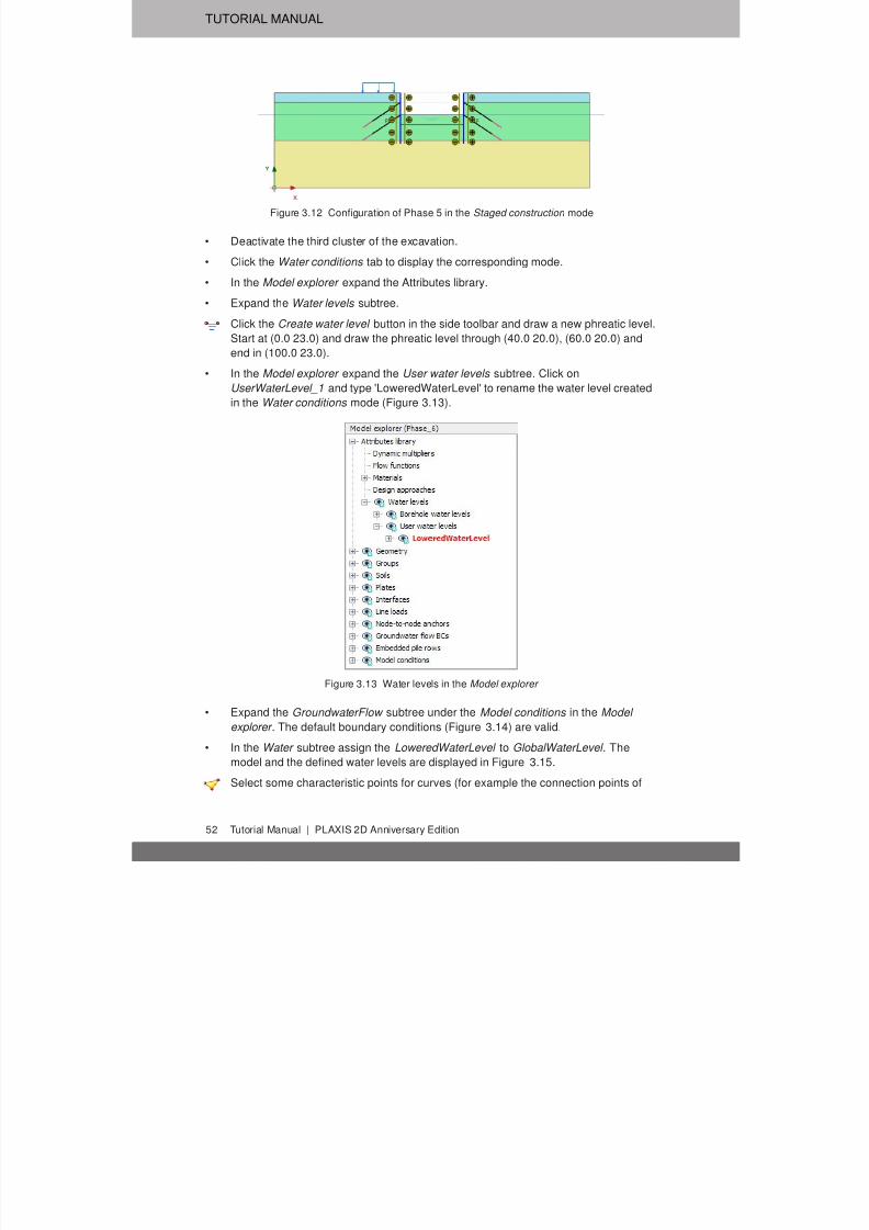
7/21/2019 2DAnniversaryEdition 1 Tutorial
http://slidepdf.com/reader/full/2danniversaryedition-1-tutorial 52/176
TUTORIAL MANUAL
Figure 3.12 Configuration of Phase 5 in the Staged construction mode
• Deactivate the third cluster of the excavation.
• Click the Water conditions tab to display the corresponding mode.
• In the Model explorer expand the Attributes library.
• Expand the Water levels subtree.
Click the Create water level button in the side toolbar and draw a new phreatic level.
Start at (0.0 23.0) and draw the phreatic level through (40.0 20.0), (60.0 20.0) and
end in (100.0 23.0).
• In the Model explorer expand the User water levels subtree. Click on
UserWaterLevel_1 and type 'LoweredWaterLevel' to rename the water level created
in the Water conditions mode (Figure 3.13).
Figure 3.13 Water levels in the Model explorer
• Expand the GroundwaterFlow subtree under the Model conditions in the Model
explorer . The default boundary conditions (Figure 3.14) are valid.
• In the Water subtree assign the LoweredWaterLevel to GlobalWaterLevel . The
model and the defined water levels are displayed in Figure 3.15.
Select some characteristic points for curves (for example the connection points of
52 Tutorial Manual | PLAXIS 2D Anniversary Edition

7/21/2019 2DAnniversaryEdition 1 Tutorial
http://slidepdf.com/reader/full/2danniversaryedition-1-tutorial 53/176
DRY EXCAVATION USING A TIE BACK WALL
Figure 3.14 The GroundwaterFlow subtree under the Model conditions in the Model explorer
Figure 3.15 Configuration of Phase 6 in the Water conditions mode
Hint: Note that for Groundwater flow (steady or transient) the intersection points of
the water level with the active model boundaries are important. The program
calculates flow boundary conditions in terms of a groundwater head
corresponding to the water level. The 'internal' part of the water level is not
used and will be replaced by the phreatic level resulting from thegroundwater flow calculation. Hence, the water level tool is just a convenient
tool to create boundary conditions for a flow calculation.
the ground anchors on the diaphragm wall, such as (40.0 27.0) and (40.0 23.0)).
Calculate the project by clicking the Calculate button in the Staged construction
mode.
Save the project after the calculation has finished.
PLAXIS 2D Anniversary Edition | Tutorial Manual 53

7/21/2019 2DAnniversaryEdition 1 Tutorial
http://slidepdf.com/reader/full/2danniversaryedition-1-tutorial 54/176
TUTORIAL MANUAL
3.4 RESULTS
Figures 3.16 to 3.20 show the deformed meshes at the end of calculation phases 2 to 6.
Figure 3.16 Deformed mesh (scaled up 50.0 times) - Phase 2
Figure 3.17 Deformed mesh (scaled up 50.0 times) - Phase 3
Figure 3.18 Deformed mesh (scaled up 50.0 times) - Phase 4
Figure 3.19 Deformed mesh (scaled up 50.0 times) - Phase 5
Figure 3.21 shows the effective principal stresses in the final situation. The passive
stress state beneath the bottom of the excavation is clearly visible. It can also be seen
54 Tutorial Manual | PLAXIS 2D Anniversary Edition
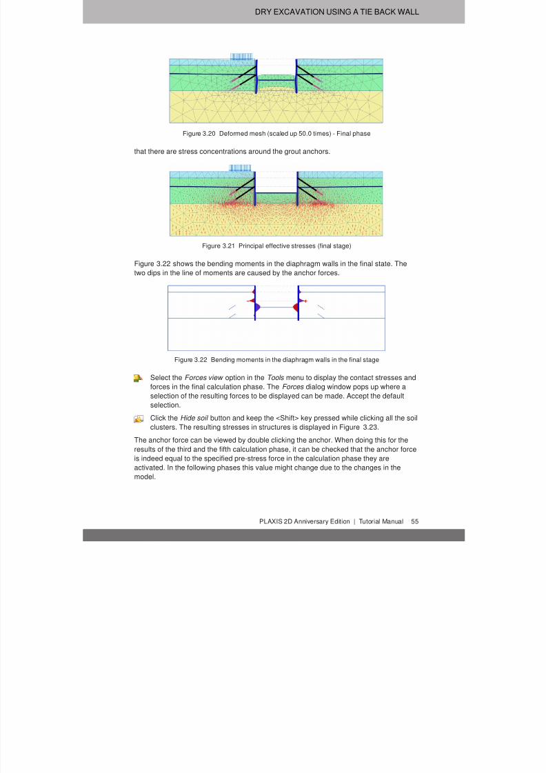
7/21/2019 2DAnniversaryEdition 1 Tutorial
http://slidepdf.com/reader/full/2danniversaryedition-1-tutorial 55/176
DRY EXCAVATION USING A TIE BACK WALL
Figure 3.20 Deformed mesh (scaled up 50.0 times) - Final phase
that there are stress concentrations around the grout anchors.
Figure 3.21 Principal effective stresses (final stage)
Figure 3.22 shows the bending moments in the diaphragm walls in the final state. The
two dips in the line of moments are caused by the anchor forces.
Figure 3.22 Bending moments in the diaphragm walls in the final stage
Select the Forces view option in the Tools menu to display the contact stresses andforces in the final calculation phase. The Forces dialog window pops up where a
selection of the resulting forces to be displayed can be made. Accept the default
selection.
Click the Hide soil button and keep the <Shift> key pressed while clicking all the soil
clusters. The resulting stresses in structures is displayed in Figure 3.23.
The anchor force can be viewed by double clicking the anchor. When doing this for the
results of the third and the fifth calculation phase, it can be checked that the anchor force
is indeed equal to the specified pre-stress force in the calculation phase they are
activated. In the following phases this value might change due to the changes in the
model.
PLAXIS 2D Anniversary Edition | Tutorial Manual 55

7/21/2019 2DAnniversaryEdition 1 Tutorial
http://slidepdf.com/reader/full/2danniversaryedition-1-tutorial 56/176
TUTORIAL MANUAL
Figure 3.23 Contact stresses in structures
56 Tutorial Manual | PLAXIS 2D Anniversary Edition

7/21/2019 2DAnniversaryEdition 1 Tutorial
http://slidepdf.com/reader/full/2danniversaryedition-1-tutorial 57/176
CONSTRUCTION OF A ROAD EMBANKMENT
4 CONSTRUCTION OF A ROAD EMBANKMENT
The construction of an embankment on soft soil with a high groundwater level leads to an
increase in pore pressure. As a result of this undrained behaviour, the effective stress
remains low and intermediate consolidation periods have to be adopted in order toconstruct the embankment safely. During consolidation the excess pore pressures
dissipate so that the soil can obtain the necessary shear strength to continue the
construction process.
This tutorial concerns the construction of a road embankment in which the mechanism
described above is analysed in detail. In the analysis three new calculation options are
introduced, namely a consolidation analysis, an updated mesh analysis and the
calculation of a safety factor by means of a safety analysis (phi/c-reduction).
4 m
3 m
3 m
12 m12 m 16 m
road embankment
peat
clay
dense sand
Figure 4.1 Situation of a road embankment on soft soil
Objectives:
• Consolidation analysis
• Modelling drains
• Change of permeability during consolidation
• Safety analysis (phi-c reduction)
• Updated mesh analysis (large deformations)
4.1 INPUT
Figure 4.1 shows a cross section of a road embankment. The embankment is 16.0 m
wide and 4.0 m high. The slopes have an inclination of 1:3. The problem is symmetric, so
only one half is modelled (in this case the right half is chosen). The embankment itself is
composed of loose sandy soil. The subsoil consists of 6.0 m of soft soil. The upper 3.0 m
is peat and the lower 3.0 m is clay. The phreatic level is located 1 m below the original
ground surface. Under the soft soil layers there is a dense sand layer of which 4.0 m are
considered in the model.
General settings
• Start the Input program and select Start a new project from the Quick select dialog
box.
• In the Project tabsheet of the Project properties window, enter an appropriate title.
• In the Model tabsheet make sure that Model is set to Plane strain and that Elements
is set to 15-Noded .
PLAXIS 2D Anniversary Edition | Tutorial Manual 57

7/21/2019 2DAnniversaryEdition 1 Tutorial
http://slidepdf.com/reader/full/2danniversaryedition-1-tutorial 58/176
TUTORIAL MANUAL
• Define the limits for the soil contour as x min = 0.0, x max = 60.0, y min = −10.0 and
y max = 4.0.
Definition of soil stratigraphy
The sub-soil layers are defined using a borehole. The embankment layers are defined in
the Structures mode. To define the soil stratigraphy:
Create a borehole at x = 0. The Modify soil layers window pops up.
• Define three soil layers as shown in Figure 4.2.
• The water level is located at y = -1 m. In the borehole column specify a value of -1 to
Head .
Open the Material sets window.
• Create soil material data sets according to Table 4.1 and assign them to the
corresponding layers in the borehole (Figure 4.2).
• Close the Modify soil layers window and proceed to the Structures mode to define
the embankment and drains.
Figure 4.2 Soil layer distribution
Hint: The initial void ratio (e init ) and the change in permeability (c k ) should be
defined to enable the modelling of a change in the permeability in a
consolidation analysis due to compression of the soil. This option is
recommended when using advanced models.
58 Tutorial Manual | PLAXIS 2D Anniversary Edition

7/21/2019 2DAnniversaryEdition 1 Tutorial
http://slidepdf.com/reader/full/2danniversaryedition-1-tutorial 59/176
CONSTRUCTION OF A ROAD EMBANKMENT
Table 4.1 Material properties of the road embankment and subsoil
Parameter Name Embankment Sand Peat Clay Unit
General
Material model Model Hardeningsoil
Hardeningsoil
Soft soil Soft soil -
Type of material behaviour Type Drained Drained Undrained
(A)
Undrained
(A)
-
Soil unit weight above
phreatic level
γ unsat 16 17 8 15 kN/m3
Soil unit weight below
phreatic level
γ sat 19 20 12 18 kN/m3
Initial void ratio e init 0.5 0.5 2.0 1.0 -
Parameters
Secant stiffness in
standard drained triaxialtest
E ref 50 2.5· 104 3.5· 104 - - kN/m2
Tangent stif fness for
primary oedometer loading
E ref oed
2.5· 104 3.5· 104 - - kN/m2
Unloading / reloading
stiffness
E ref ur 7.5· 104 1.05· 105 - - kN/m2
Power for stress-level
dependency of stiffness
m 0.5 0.5 - - -
Modified compression
index
λ∗ - - 0.15 0.05 -
Modified swelling index κ∗ - - 0.03 0.01 -
Cohesion c ref ' 1.0 0.0 2.0 1.0 kN/m2
Friction angle ϕ' 30 33 23 25 ◦
Dilatancy angle ψ 0.0 3.0 0 0 ◦
Advanced: Set to default Yes Yes Yes Yes Yes Yes
Flow parameters
Data set - USDA USDA USDA USDA -
Model - Van
Genuchten
Van
Genuchten
Van
Genuchten
Van
Genuchten
-
Soil type - Loamy sand Sand Clay Clay -
> 2µm - 6.0 4.0 70.0 70.0 %
2µm − 50µm - 11.0 4.0 13.0 13.0 %
50µm − 2mm - 83.0 92.0 17.0 17.0 %
Set to default - Yes Yes No Yes -
Horizontal permeability k x 3.499 7.128 0.1 0.04752 m/day
Vertical permeability k y 3.499 7.128 0.05 0.04752 m/day
Change in permeability c k 1· 1015 1· 1015 1.0 0.2 -
Interfaces
Interface strength − Rigid Rigid Rigid Rigid -
Strength reduction factor R inter 1.0 1.0 1.0 1.0 -
Initial
K 0 determination − Automatic Automatic Automatic Automatic -
Over-consolidation ratio OCR 1.0 1.0 1.0 1.0 -
Pre-overburden pressure POP 0.0 0.0 5.0 0.0 kN/m2
PLAXIS 2D Anniversary Edition | Tutorial Manual 59

7/21/2019 2DAnniversaryEdition 1 Tutorial
http://slidepdf.com/reader/full/2danniversaryedition-1-tutorial 60/176
TUTORIAL MANUAL
4.1.1 DEFINITION OF EMBANKMENT AND DRAINS
The embankment and the drains are defined in the Structures mode. To define the
embankment layers:
Click the Create soil polygon button in the side toolbar and select the Create soil polygon option in the appearing menu.
• Define the embankment in the draw area by clicking on (0.0 0.0), (0.0 4.0), (8.0 4.0)
and (20.0 0.0).
• Right-click the created polygon and assign the Embankment data set to the soil
polygon (Figure 4.3).
Figure 4.3 Assignment of a material dataset to a soil cluster in the draw area
To define the embankment construction level click the Cut polygon in the side
toolbar and define a cutting line by clicking on (0.0 2.0) and (14.0 2.0). The
embankment cluster is split into two sub-clusters.
In this project the effect of the drains on the consolidation time will be investigated by
comparing the results with a case without drains. Drains will only be active for the
calculation phases in the case with drains.
Click the Create hydraulic conditions button in the side toolbar and select the Create
drain option in the appearing menu (Figure 4.4).
Figure 4.4 The Create drain option in the Create hydraulic conditions menu
Drains are defined in the soft layers (clay and peat; y = 0.0 to y = -6.0). The distance
between two consecutive drains is 2 m. Considering the symmetry, the first drain is
located at 1 m distance from the model boundary. 10 drains will be created in total
(Figure 4.5)
60 Tutorial Manual | PLAXIS 2D Anniversary Edition

7/21/2019 2DAnniversaryEdition 1 Tutorial
http://slidepdf.com/reader/full/2danniversaryedition-1-tutorial 61/176
CONSTRUCTION OF A ROAD EMBANKMENT
Figure 4.5 Final geometry of the model
4.2 MESH GENERATION
• Proceed to the Mesh mode.
Generate the mesh. Use the default option for the Element distribution parameter
(Medium ).
View the generated mesh. The resulting mesh is shown in Figure 4.6.• Click on the Close tab to close the Output program.
Figure 4.6 The generated mesh
4.3 CALCULATIONS
The embankment construction is divided into two phases. After the first construction
phase a consolidation period of 30 days is introduced to allow the excess pore pressures
to dissipate. After the second construction phase another consolidation period is
introduced from which the final settlements may be determined. Hence, a total of four
calculation phases have to be defined besides the initial phase.
Initial phase: Initial conditions
In the initial situation the embankment is not present. In order to generate the initial
stresses therefore, the embankment must be deactivated first in the Staged construction
mode.
• In the Staged construction mode deactivate the two clusters that represent the
embankment, just like in a staged construction calculation. When the embankment
has been deactivated (the corresponding clusters should have the background
colour), the remaining active geometry is horizontal with horizontal layers, so the K0
procedure can be used to calculate the initial stresses (Figure 4.7).
PLAXIS 2D Anniversary Edition | Tutorial Manual 61

7/21/2019 2DAnniversaryEdition 1 Tutorial
http://slidepdf.com/reader/full/2danniversaryedition-1-tutorial 62/176
TUTORIAL MANUAL
Figure 4.7 Configuration of the initial phase
The initial water pressures are fully hydrostatic and based on a general phreatic level
located at y = -1. Note that a phreatic level is automatically created at y = -1, according to
the value specified for Head in the borehole. In addition to the phreatic level, attention
must be paid to the boundary conditions for the consolidation analysis that will be
performed during the calculation process. Without giving any additional input, all
boundaries except for the bottom boundary are draining so that water can freely flow out
of these boundaries and excess pore pressures can dissipate. In the current situation,however, the left vertical boundary must be closed because this is a line of symmetry, so
horizontal flow should not occur. The remaining boundaries are open because the excess
pore pressures can be dissipated through these boundaries. In order to define the
appropriate consolidation boundary conditions, follow these steps:
• In the Model explorer expand the Model conditions subtree.
• Expand the GroundwaterFlow subtree and set BoundaryXMin to Closed and
BoundaryYMin to Open (Figure 4.8).
Figure 4.8 The boundary conditions of the problem
Consolidation analysis
A consolidation analysis introduces the dimension of time in the calculations. In order to
correctly perform a consolidation analysis a proper time step must be selected. The use
of time steps that are smaller than a critical minimum value can result in stressoscillations.
The consolidation option in PLAXIS allows for a fully automatic time stepping procedure
62 Tutorial Manual | PLAXIS 2D Anniversary Edition

7/21/2019 2DAnniversaryEdition 1 Tutorial
http://slidepdf.com/reader/full/2danniversaryedition-1-tutorial 63/176
CONSTRUCTION OF A ROAD EMBANKMENT
that takes this critical time step into account. Within this procedure there are three main
possibilities:
Consolidate for a predefined period, including the effects of changes to the active
geometry (Staged construction ).
Consolidate until all excess pore pressures in the geometry have reduced to a
predefined minimum value (Minimum excess pore pressure ).
Consolidate until a specified degree of saturation is reached (Degree of
consolidation ).
The first two possibilities will be used in this exercise. To define the calculation phases,
follow these steps:
Phase 1: The first calculation stage is a Consolidation analysis, Staged construction .
Add a new phase.
In the Phases window select the Consolidation option from the Calculation type
drop-down menu in the General subtree.
Make sure that the Staged construction option is selected for the Loading type .
• Enter a Time interval of 2 days. The default values of the remaining parameters will
be used.
• In the Staged construction mode activate the first part of the embankment (Figure
4.9).
Figure 4.9 Configuration of the phase 1
Phase 2: The second phase is also a Consolidation analysis, Staged construction . In
this phase no changes to the geometry are made as only a consolidation analysis to
ultimate time is required.
Add a new phase.
In the Phases window select the Consolidation option from the Calculation type
drop-down menu in the General subtree.
Make sure that the Staged construction option is selected for the Loading type .
• Enter a Time interval of 30 days. The default values of the remaining parameters will
be used.
Phase 3: The third phase is once again a Consolidation analysis, Staged construction .
Add a new phase.
In the Phases window select the Consolidation option from the Calculation type
drop-down menu in the General subtree.
PLAXIS 2D Anniversary Edition | Tutorial Manual 63

7/21/2019 2DAnniversaryEdition 1 Tutorial
http://slidepdf.com/reader/full/2danniversaryedition-1-tutorial 64/176
TUTORIAL MANUAL
Make sure that the Staged construction option is selected for the Loading type .
• Enter a Time interval of 1 day. The default values of the remaining parameters will
be used.
• In the Staged construction mode activate the second part of the embankment(Figure 4.10).
Figure 4.10 Configuration of the phase 3
Phase 4: The fourth phase is a Consolidation analysis to a minimum excess pore
pressure.
Add a new phase.
In the General subtree select the Consolidation as calculation type.
Select the Minimum excess pore pressure option in the Loading input drop-down
menu and accept the default value of 1 kN/m2 for the minimum pressure. The
default values of the remaining parameters will be used.
Before starting the calculation, click the Select points for curves button and select
the following points: As Point A, select the toe of the embankment. The secondpoint (Point B) will be used to plot the development (and decay) of excess pore pressures.
To this end, a point somewhere in the middle of the soft soil layers is needed, close to
(but not actually on) the left boundary. After selecting these points, start the calculation.
During a consolidation analysis the development of time can be viewed in the upper part
of the calculation info window (Figure 4.11).
In addition to the multipliers, a parameter P excess ,max occurs, which indicates the current
maximum excess pore pressure. This parameter is of interest in the case of a Minimum
excess pore pressure consolidation analysis, where all pore pressures are specified to
reduce below a predefined value.
64 Tutorial Manual | PLAXIS 2D Anniversary Edition
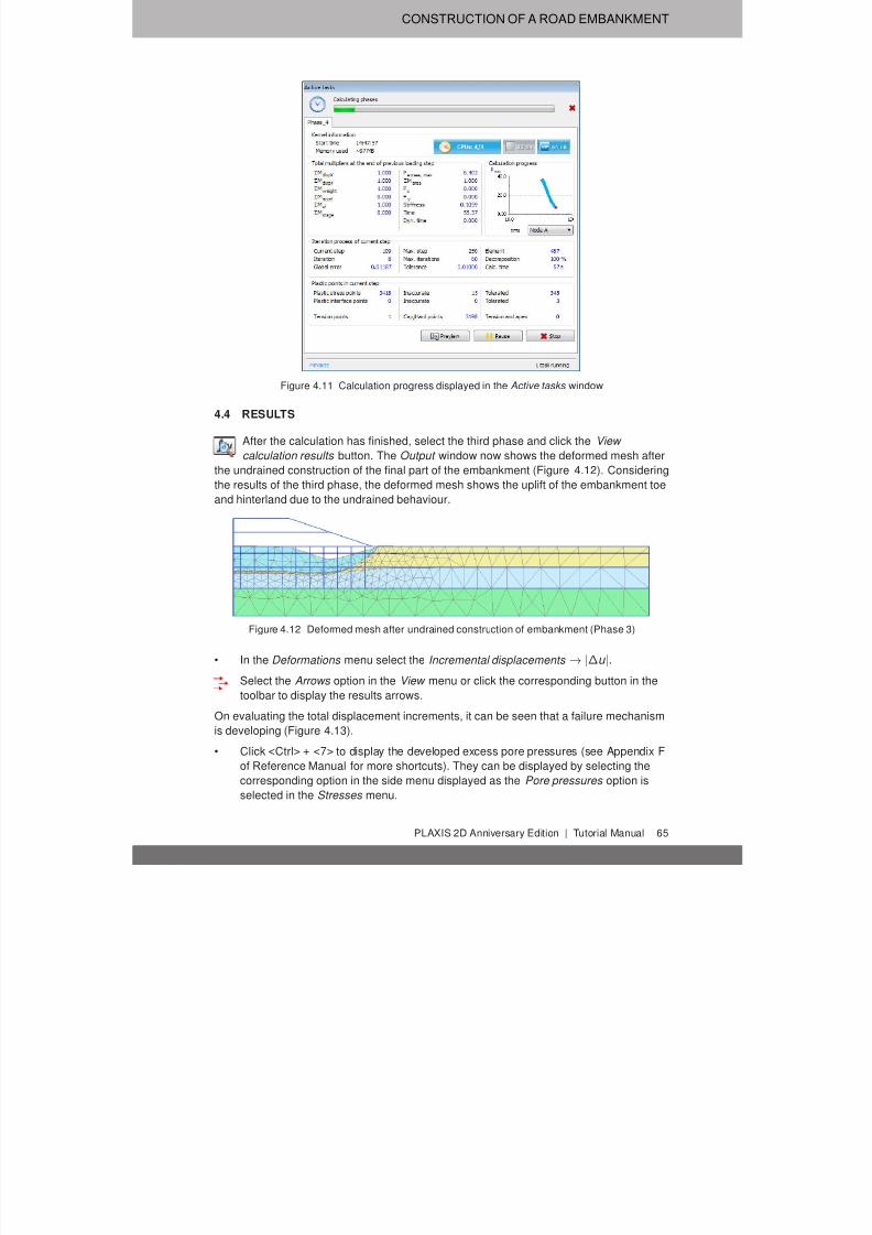
7/21/2019 2DAnniversaryEdition 1 Tutorial
http://slidepdf.com/reader/full/2danniversaryedition-1-tutorial 65/176
CONSTRUCTION OF A ROAD EMBANKMENT
Figure 4.11 Calculation progress displayed in the Active tasks window
4.4 RESULTS
After the calculation has finished, select the third phase and click the View
calculation results button. The Output window now shows the deformed mesh afterthe undrained construction of the final part of the embankment (Figure 4.12). Considering
the results of the third phase, the deformed mesh shows the uplift of the embankment toe
and hinterland due to the undrained behaviour.
Figure 4.12 Deformed mesh after undrained construction of embankment (Phase 3)
• In the Deformations menu select the Incremental displacements → |∆u |.
Select the Arrows option in the View menu or click the corresponding button in the
toolbar to display the results arrows.
On evaluating the total displacement increments, it can be seen that a failure mechanism
is developing (Figure 4.13).
• Click <Ctrl> + <7> to display the developed excess pore pressures (see Appendix F
of Reference Manual for more shortcuts). They can be displayed by selecting the
corresponding option in the side menu displayed as the Pore pressures option is
selected in the Stresses menu.
PLAXIS 2D Anniversary Edition | Tutorial Manual 65

7/21/2019 2DAnniversaryEdition 1 Tutorial
http://slidepdf.com/reader/full/2danniversaryedition-1-tutorial 66/176
TUTORIAL MANUAL
Figure 4.13 Displacement increments after undrained construction of embankment
Click the Center principal directions . The principal directions of excess pressures
are displayed at the center of each soil element. The results are displayed in Figure
4.14. It is clear that the highest excess pore pressure occurs under the embankment
centre.
Figure 4.14 Excess pore pressures after undrained construction of embankment
• Select Phase 4 in the drop down menu.
Click the Contour lines button in the toolbar to display the results as contours.
Use the Draw scanline button or the corresponding option in the View menu to
define the position of the contour line labels.
Figure 4.15 Excess pore pressure contours after consolidation to P excess < 1.0 kN/m2
It can be seen that the settlement of the original soil surface and the embankment
increases considerably during the fourth phase. This is due to the dissipation of the
excess pore pressures (= consolidation), which causes further settlement of the soil.
Figure 4.15 shows the remaining excess pore pressure distribution after consolidation.
Check that the maximum value is below 1.0 kN/m2.
The Curves manager can be used to view the development, with time, of the excess pore
pressure under the embankment. In order to create such a curve, follow these steps:
Create a new curve.
66 Tutorial Manual | PLAXIS 2D Anniversary Edition

7/21/2019 2DAnniversaryEdition 1 Tutorial
http://slidepdf.com/reader/full/2danniversaryedition-1-tutorial 67/176
CONSTRUCTION OF A ROAD EMBANKMENT
• For the x -axis, select the Project option from the drop-down menu and select Time
in the tree.
• For the y -axis select the point in the middle of the soft soil layers (Point B) from the
drop-down menu. In the tree select Stresses → Pore pressure → p excess .
• Select the Invert sign option for y-axis. After clicking the OK button, a curve similar
to Figure 4.16 should appear.
Figure 4.16 Development of excess pore pressure under the embankment
Figure 4.16 clearly shows the four calculation phases. During the construction phases
the excess pore pressure increases with a small increase in time while during the
consolidation periods the excess pore pressure decreases with time. In fact,
consolidation already occurs during construction of the embankment, as this involves a
small time interval. From the curve it can be seen that more than 50 days are needed to
reach full consolidation.
• Save the chart before closing the Output program.
4.5 SAFETY ANALYSIS
In the design of an embankment it is important to consider not only the final stability, but
also the stability during the construction. It is clear from the output results that a failure
mechanism starts to develop after the second construction phase.
It is interesting to evaluate a global safety factor at this stage of the problem, and also for
other stages of construction.
In structural engineering, the safety factor is usually defined as the ratio of the collapse
load to the working load. For soil structures, however, this definition is not always useful.
For embankments, for example, most of the loading is caused by soil weight and anincrease in soil weight would not necessarily lead to collapse. Indeed, a slope of purely
frictional soil will not fail in a test in which the self weight of the soil is increased (like in a
PLAXIS 2D Anniversary Edition | Tutorial Manual 67
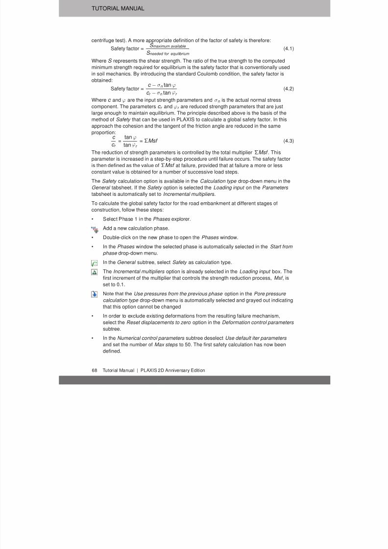
7/21/2019 2DAnniversaryEdition 1 Tutorial
http://slidepdf.com/reader/full/2danniversaryedition-1-tutorial 68/176
TUTORIAL MANUAL
centrifuge test). A more appropriate definition of the factor of safety is therefore:
Safety factor = S maximum available
S needed for equilibrium
(4.1)
Where S represents the shear strength. The ratio of the true strength to the computed
minimum strength required for equilibrium is the safety factor that is conventionally usedin soil mechanics. By introducing the standard Coulomb condition, the safety factor is
obtained:
Safety factor = c − σn tan ϕ
c r −σn tan ϕr
(4.2)
Where c and ϕ are the input strength parameters and σn is the actual normal stress
component. The parameters c r and ϕr are reduced strength parameters that are just
large enough to maintain equilibrium. The principle described above is the basis of the
method of Safety that can be used in PLAXIS to calculate a global safety factor. In this
approach the cohesion and the tangent of the friction angle are reduced in the same
proportion:c
c r =
tanϕ
tanϕr
= ΣMsf (4.3)
The reduction of strength parameters is controlled by the total multiplier ΣMsf . This
parameter is increased in a step-by-step procedure until failure occurs. The safety factor
is then defined as the value of ΣMsf at failure, provided that at failure a more or less
constant value is obtained for a number of successive load steps.
The Safety calculation option is available in the Calculation type drop-down menu in the
General tabsheet. If the Safety option is selected the Loading input on the Parameters
tabsheet is automatically set to Incremental multipliers .
To calculate the global safety factor for the road embankment at different stages ofconstruction, follow these steps:
• Select Phase 1 in the Phases explorer.
Add a new calculation phase.
• Double-click on the new phase to open the Phases window.
• In the Phases window the selected phase is automatically selected in the Start from
phase drop-down menu.
In the General subtree, select Safety as calculation type.
The Incremental multipliers option is already selected in the Loading input box. Thefirst increment of the multiplier that controls the strength reduction process, Msf , is
set to 0.1.
Note that the Use pressures from the previous phase option in the Pore pressure
calculation type drop-down menu is automatically selected and grayed out indicating
that this option cannot be changed
• In order to exclude existing deformations from the resulting failure mechanism,
select the Reset displacements to zero option in the Deformation control parameters
subtree.
• In the Numerical control parameters subtree deselect Use default iter parameters and set the number of Max steps to 50. The first safety calculation has now been
defined.
68 Tutorial Manual | PLAXIS 2D Anniversary Edition

7/21/2019 2DAnniversaryEdition 1 Tutorial
http://slidepdf.com/reader/full/2danniversaryedition-1-tutorial 69/176
CONSTRUCTION OF A ROAD EMBANKMENT
• Follow the same steps to create new calculation phases that analyse the stability at
the end of each consolidation phase.
Hint: The default value of Max steps in a Safety calculation is 100. In contrast toan Staged construction calculation, the specified number of steps is always
fully executed. In most Safety calculations, 100 steps are sufficient to arrive
at a state of failure. If not, the number of steps can be increased to a
maximum of 1000.
» For most Safety analyses Msf = 0.1 is an adequate first step to start up the
process. During the calculation process, the development of the total
multiplier for the strength reduction, ΣMsf , is automatically controlled by the
load advancement procedure.
Figure 4.17 Phases explorer displaying the Safety calculation phases
Evaluation of results
Additional displacements are generated during a Safety calculation. The total
displacements do not have a physical meaning, but the incremental displacements in the
final step (at failure) give an indication of the likely failure mechanism.
In order to view the mechanisms in the three different stages of the embankment
construction:
Select one of these phases and click the View calculation results button.
• From the Deformations menu select Incremental displacements → |∆u |.
Change the presentation from Arrows to Shadings . The resulting plots give a good
impression of the failure mechanisms (Figure 4.18). The magnitude of the
displacement increments is not relevant.
The safety factor can be obtained from the Calculation info option of the Project menu.
The Multipliers tabsheet of the Calculation information window represents the actual
values of the load multipliers. The value of ΣMsf represents the safety factor, provided
that this value is indeed more or less constant during the previous few steps.
The best way to evaluate the safety factor, however, is to plot a curve in which the
parameter ΣMsf is plotted against the displacements of a certain node. Although the
displacements are not relevant, they indicate whether or not a failure mechanism has
PLAXIS 2D Anniversary Edition | Tutorial Manual 69
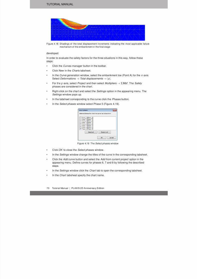
7/21/2019 2DAnniversaryEdition 1 Tutorial
http://slidepdf.com/reader/full/2danniversaryedition-1-tutorial 70/176
TUTORIAL MANUAL
Figure 4.18 Shadings of the total displacement increments indicating the most applicable failure
mechanism of the embankment in the final stage
developed.
In order to evaluate the safety factors for the three situations in this way, follow these
steps:
• Click the Curves manager button in the toolbar.
• Click New in the Charts tabsheet.
• In the Curve generation window, select the embankment toe (Point A) for the x -axis.
Select Deformations → Total displacements → |u |.
• For the y -axis, select Project and then select Multipliers → ΣMsf . The Safety
phases are considered in the chart.
• Right-click on the chart and select the Settings option in the appearing menu. The
Settings window pops up.
• In the tabsheet corresponding to the curve click the Phases button.
• In the Select phases window select Phase 5 (Figure 4.19).
Figure 4.19 The Select phases window
• Click OK to close the Select phases window.
• In the Settings window change the titles of the curve in the corresponding tabsheet.
• Click the Add curve button and select the Add from current project option in the
appearing menu. Define curves for phases 6, 7 and 8 by following the described
steps.
• In the Settings window click the Chart tab to open the corresponding tabsheet.• In the Chart tabsheet specify the chart name.
70 Tutorial Manual | PLAXIS 2D Anniversary Edition

7/21/2019 2DAnniversaryEdition 1 Tutorial
http://slidepdf.com/reader/full/2danniversaryedition-1-tutorial 71/176
CONSTRUCTION OF A ROAD EMBANKMENT
• Set the scaling of the x-axis to Manual and set the value of Maximum to 1 (Figure
4.20).
Figure 4.20 The Chart tabsheet in the Settings window
• Click Apply to update the chart according to the changes made and click OK to
close the Settings window.
• To modify the location of the legend right-click on the legend.
• In the appearing menu point at View and select the Legend in chart option (Figure4.21).
Figure 4.21 Enabling legend in chart
• The legend can be relocated in the chart by dragging it. The plot is shown in Figure
4.22.
The maximum displacements plotted are not relevant. It can be seen that for all curves a
more or less constant value of ΣMsf is obtained. Hovering the mouse cursor over a point
on the curves, a box showing the exact value of ΣMsf can be obtained.
PLAXIS 2D Anniversary Edition | Tutorial Manual 71
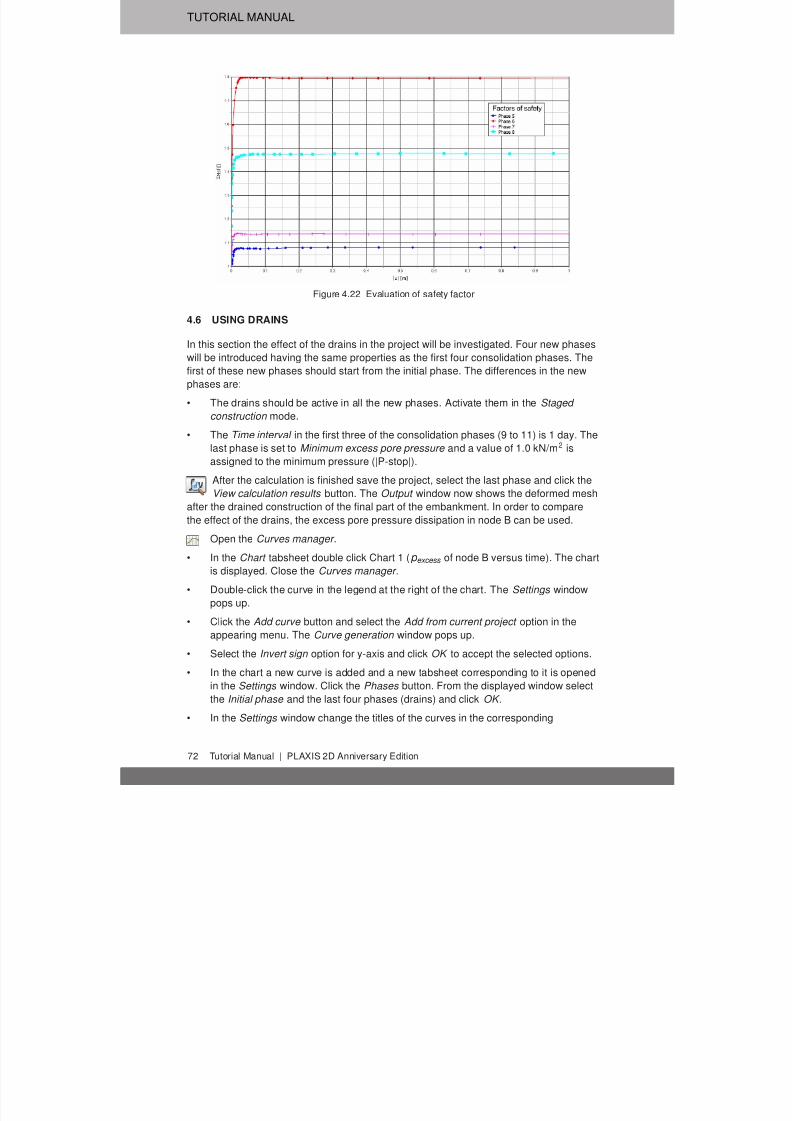
7/21/2019 2DAnniversaryEdition 1 Tutorial
http://slidepdf.com/reader/full/2danniversaryedition-1-tutorial 72/176
TUTORIAL MANUAL
Figure 4.22 Evaluation of safety factor
4.6 USING DRAINS
In this section the effect of the drains in the project will be investigated. Four new phases
will be introduced having the same properties as the first four consolidation phases. The
first of these new phases should start from the initial phase. The differences in the new
phases are:
• The drains should be active in all the new phases. Activate them in the Staged
construction mode.
• The Time interval in the first three of the consolidation phases (9 to 11) is 1 day. The
last phase is set to Minimum excess pore pressure and a value of 1.0 kN/m2 is
assigned to the minimum pressure (|P-stop|).
After the calculation is finished save the project, select the last phase and click the
View calculation results button. The Output window now shows the deformed mesh
after the drained construction of the final part of the embankment. In order to compare
the effect of the drains, the excess pore pressure dissipation in node B can be used.
Open the Curves manager .
• In the Chart tabsheet double click Chart 1 (p excess of node B versus time). The chart
is displayed. Close the Curves manager .
• Double-click the curve in the legend at the right of the chart. The Settings window
pops up.
• Click the Add curve button and select the Add from current project option in the
appearing menu. The Curve generation window pops up.
• Select the Invert sign option for y-axis and click OK to accept the selected options.
• In the chart a new curve is added and a new tabsheet corresponding to it is opened
in the Settings window. Click the Phases button. From the displayed window selectthe Initial phase and the last four phases (drains) and click OK .
• In the Settings window change the titles of the curves in the corresponding
72 Tutorial Manual | PLAXIS 2D Anniversary Edition

7/21/2019 2DAnniversaryEdition 1 Tutorial
http://slidepdf.com/reader/full/2danniversaryedition-1-tutorial 73/176
CONSTRUCTION OF A ROAD EMBANKMENT
tabsheets.
• In the Chart tabsheet specify the chart name.
• Click Apply to preview the generated cure and click OK to close the Settings
window. The chart (Figure 4.23) gives a clear view of the effect of drains in the timerequired for the excess pore pressures to dissipate.
Figure 4.23 Effect of drains
Hint: Instead of adding a new curve, the existing curve can be regenerated using
the corresponding button in the Curves settings window.
4.7 UPDATED MESH + UPDATED WATER PRESSURES ANALYSIS
As can be seen from the output of the Deformed mesh at the end of consolidation (stage
4), the embankment settles about one meter since the start of construction. Part of the
sand fill that was originally above the phreatic level will settle below the phreatic level.As a result of buoyancy forces the effective weight of the soil that settles below the water
level will change, which leads to a reduction of the effective overburden in time. This
effect can be simulated in PLAXIS using the Updated mesh and Updated water pressures
options. For the road embankment the effect of using these options will be investigated.
• Select the initial phase in the Phases explorer.
Add a new calculation phase.
• Define the new phase in the same way as Phase 1. In the Deformation control
parameters subtree check the Updated mesh and Updated water pressures options.
• Define in the same way the other 3 phases.
When the calculation has finished, compare the settlements for the two different
PLAXIS 2D Anniversary Edition | Tutorial Manual 73

7/21/2019 2DAnniversaryEdition 1 Tutorial
http://slidepdf.com/reader/full/2danniversaryedition-1-tutorial 74/176
TUTORIAL MANUAL
calculation methods.
• In the Curve generation window select time for the x -axis and select the vertical
displacement (u y ) of the point in the middle of the soft soil layers (Point B) for the
y -axis.
• In this curve the results for Initial phase and phases from 1 to 4 will be considered.
• Add a new curve to the chart.
• In this curve the results for Initial phase and phases from 13 to 16 will be
considered. The resulting chart is shown in Figure 4.24.
Figure 4.24 Effect of Updated mesh and water pressures analysis on resulting settlements
In Figure 4.24 it can be seen that the settlements are less when the Updated mesh and
Updated water pressures options are used (red curve). This is partly because the
Updated mesh procedure includes second order deformation effects by which changes of
the geometry are taken into account, and partly because the Updated water pressures
procedure results in smaller effective weights of the embankment. This last effect is
caused by the buoyancy of the soil settling below the (constant) phreatic level. The use of
these procedures allows for a realistic analysis of settlements, taking into account the
positive effects of large deformations.
74 Tutorial Manual | PLAXIS 2D Anniversary Edition
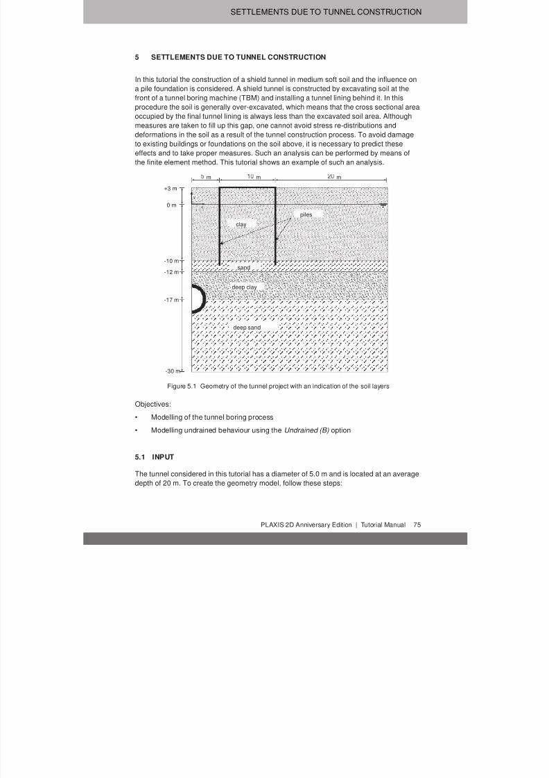
7/21/2019 2DAnniversaryEdition 1 Tutorial
http://slidepdf.com/reader/full/2danniversaryedition-1-tutorial 75/176
SETTLEMENTS DUE TO TUNNEL CONSTRUCTION
5 SETTLEMENTS DUE TO TUNNEL CONSTRUCTION
In this tutorial the construction of a shield tunnel in medium soft soil and the influence on
a pile foundation is considered. A shield tunnel is constructed by excavating soil at the
front of a tunnel boring machine (TBM) and installing a tunnel lining behind it. In thisprocedure the soil is generally over-excavated, which means that the cross sectional area
occupied by the final tunnel lining is always less than the excavated soil area. Although
measures are taken to fill up this gap, one cannot avoid stress re-distributions and
deformations in the soil as a result of the tunnel construction process. To avoid damage
to existing buildings or foundations on the soil above, it is necessary to predict these
effects and to take proper measures. Such an analysis can be performed by means of
the finite element method. This tutorial shows an example of such an analysis.
x
y
+3 m
0 m
-10 m
-12 m
-17 m
-30 m
m m m
clay
piles
sand
deep clay
deep sand
Figure 5.1 Geometry of the tunnel project with an indication of the soil layers
Objectives:
• Modelling of the tunnel boring process
• Modelling undrained behaviour using the Undrained (B) option
5.1 INPUT
The tunnel considered in this tutorial has a diameter of 5.0 m and is located at an average
depth of 20 m. To create the geometry model, follow these steps:
PLAXIS 2D Anniversary Edition | Tutorial Manual 75

7/21/2019 2DAnniversaryEdition 1 Tutorial
http://slidepdf.com/reader/full/2danniversaryedition-1-tutorial 76/176
TUTORIAL MANUAL
General settings
• Start the Input program and select Start a new project from the Quick select dialog
box.
• In the Project tabsheet of the Project properties window, enter an appropriate title.• In the Model tabsheet keep the default options for Model (Plane strain ), and
Elements (15-Noded ).
• Keep the default values for units and the general parameters.
• Set the model dimensions to x min = 0.0 m, x max = 35.0 m, y min = -30.0 m, y max = 3.0
m and press OK to close the Project properties window.
Definition of soil stratigraphy
The soil profile indicates four distinct layers: The upper 13 m consists of soft clay type
soil with stiffness that increases approximately linearly with depth. Under the clay layerthere is a 2.0 m thick fine sand layer. This layer is used as a foundation layer for old
wooden piles on which traditional brickwork houses were built. The pile foundation of
such a building is modelled next to the tunnel. Displacements of these piles may cause
damage to the building, which is highly undesirable. Below the sand layer there is a 5.0 m
thick deep loamy clay layer.
To define the soil stratigraphy:
Create a borehole at x = 0. The Modify soil layers window pops up.
• Create the soil stratigraphy as shown in Figure 5.2.
Figure 5.2 The soil stratigraphy in the Modify soil layers window
• Keep the Head in the borehole at 0.0 m.
Open the Material sets window.• Create data sets under the Soil and interfaces set type according to the information
given in Table 5.1.
76 Tutorial Manual | PLAXIS 2D Anniversary Edition

7/21/2019 2DAnniversaryEdition 1 Tutorial
http://slidepdf.com/reader/full/2danniversaryedition-1-tutorial 77/176
SETTLEMENTS DUE TO TUNNEL CONSTRUCTION
Table 5.1 Material properties of soil in the tunnel project
Parameter Name Clay Sand Deep clay Deep sand Unit
General
Material model Model Mohr-Coulomb
Hardeningsoil
Mohr-Coulomb
HS small -
Drainage type Type Undrained(B)
Drained Undrained(B)
Drained -
Soil unit weight above p.l. γ unsat 15 16.5 16 17 kN/m3
Soil unit weight below p.l. γ sat 18 20 18.5 21 kN/m3
Parameters
Young's modulus at referencelevel
E ' 3.4·103 - 9.0· 103 - kN/m2
Secant stiffness in standarddrained triaxial test
E ref 50 - 2.5· 104 - 4.2· 104 kN/m2
Tangent stiffness for primaryoedometer loading
E ref oed - 2.5· 104 - 4.2· 104 kN/m2
Unloading / reloading stiffness E ref ur - 7.5· 104 - 1.26· 105 kN/m2
Power for stress-leveldependency of stiffness
m - 0.5 - 0.5 -
Cohesion c 'ref - 0 - 0 kN/m2
Undrained shear strength atreference level
s u ,ref 5 - 40 - kN/m2
Friction angle ϕ' - 31 - 35 ◦
Dilatancy angle ψ - 1.0 - 5 ◦
Shear strain at which G s =0.722G 0
γ 0.7 - - - 1.3·10-4 -
Shear modulus at very smallstrains
G ref 0 - - - 1.1· 105 kN/m2
Poisson's ratio ν ' 0.33 0.3 0.33 0.3 -
Young's modulus inc. E 'inc 400 - 600 - kN/m3
Reference level y ref
3.0 - -12 - m
Undrained shear strength inc. s u ,inc 2 - 3 - kN/m2
Reference level y ref 3.0 - -12 - m
Flow parameters
Horizontal permeability k x 1·10-4 1.0 1·10-2 0.5 m/day
Vertical permeability k y 1·10-4 1.0 1·10-2 0.5 m/day
Interfaces
Interface strength type Type Rigid Rigid Manual Manual -
Interface strength R inter 1.0 1.0 0.7 0.7 -
Initial
K 0 determination − Manual Automatic Manual Automatic -
Lateral ear th pressure
coefficient
K 0,x 0.60 0.485 0.60 0.4264 -
Over-consolidation ratio OCR - 1.0 - 1.0 -
Pre-overburden ratio POP - 0.0 - 0.0 -
For the upper clay layer the stiffness and shear strength increase with depth. Therefore
values for E 'inc and s u ,inc are entered in the Advanced subtree. The values of E 'ref and
s u ,ref become the reference values at the reference level y ref . Below y ref , the actual
values of E ' and s u , increase with depth according to:
E '(y ) = E 'ref + E 'inc (y ref − y )
s u (y ) = s u ,ref + s u ,inc (y ref − y )
The data sets of the two lower soil layers include appropriate parameters for the tunnelinterfaces. In the other data sets the interface properties just remain at their default
values. Enter four data sets with the properties as listed in Table 5.1 and assign them to
PLAXIS 2D Anniversary Edition | Tutorial Manual 77

7/21/2019 2DAnniversaryEdition 1 Tutorial
http://slidepdf.com/reader/full/2danniversaryedition-1-tutorial 78/176
TUTORIAL MANUAL
the corresponding clusters in the geometry model.
5.1.1 DEFINITION OF STRUCTURAL ELEMENTS
The tunnel considered here is the right half of a circular tunnel and will be composed offour sections. After generating the basic geometry, follow these steps to design the
circular tunnel:
In the Structures mode click the Create tunnel button in the side toolbar and click at
(0.0 -17.0) in the draw area. The Tunnel designer window pops up displaying the
General tabsheet of the Cross section mode.
• Select the Circular option in the Shape type drop-down menu.
• Select the Define right half option in the Whole or half tunnel drop-down menu.
• In the Offset to begin point group set Axis 2 to -2.5. No change is required for the
orientation axes.
• Click the Segments tab to proceed to the corresponding tabsheet. A segment is
automatically created. A new box is shown under the segment list where the
properties of the segment can be defined.
• In the Segment box set Radius to 2.5 m. The generated segment is shown in Figure
5.3.
Figure 5.3 The geometry of the tunnel segment
• Click the Properties tab to proceed to the corresponding tabsheet.
• Right-click the segment in the display area and select the Create plate option in the
appearing menu.
• In the Polycurve box expand the Plate subtree.Create a new material dataset. Specify the material parameters for lining according
to Table 5.2.
78 Tutorial Manual | PLAXIS 2D Anniversary Edition

7/21/2019 2DAnniversaryEdition 1 Tutorial
http://slidepdf.com/reader/full/2danniversaryedition-1-tutorial 79/176
SETTLEMENTS DUE TO TUNNEL CONSTRUCTION
Hint: In the tunnel as considered here the segments do not have a specific
meaning as the tunnel lining is homogeneous and the tunnel will be
constructed at once. In general, the meaning of segments becomes
significant when:• It is desired to excavate or construct the tunnel (lining) in different
stages.
• Different tunnel segments have different lining properties.
• One would consider hinge connections in the lining (hinges can be
added after the design of the tunnel in the general draw area).
• The tunnel shape is composed of arcs with different radii (for example
NATM tunnels).
Table 5.2 Material properties of the plates
Parameter Name Lining Building Unit
Material type Type Elastic;Isotropic
Elastic;Isotropic
-
Normal stiffness EA 1.4·107 1·1010 kN/m
Flexural rigidity EI 1.43·105 1·1010 kNm2 /m
Weight w 8.4 25 kN/m/m
Poisson's ratio ν 0.15 0.0 -
Hint: A tunnel lining consists of curved plates (shells). The lining properties can be
specified in the material database for plates. Similarly, a tunnel interface is
nothing more than a curved interface.
• Right-click the segment in the display area and select the Create negative interface
option in the appearing menu.
• Right-click the segment in the display area and select the Create line contraction
option in the appearing menu. In the polycurve box expand the Contractions subtree
and specify a value of 0.5%. The tunnel model is shown in Figure 5.4.
Hint: A line contraction of the tunnel contour of 0.5% corresponds approximately toa value loss of 1% of the tunnel volume.
• Click on Generate to include the defined tunnel in the model.
• Close the Tunnel designer window.
The building itself will be represented by a stiff plate founded on piles.
Draw a plate from (5.0 3.0) to (15.0 3.0), representing the building.
Create a material set for the building according to Table 5.2 and assign it to the plate.
Draw two piles (embedded pile row) from (5.0 3.0) to (5.0 -11.0) and from (15.0 3.0)to (15.0 -11.0).
PLAXIS 2D Anniversary Edition | Tutorial Manual 79

7/21/2019 2DAnniversaryEdition 1 Tutorial
http://slidepdf.com/reader/full/2danniversaryedition-1-tutorial 80/176
TUTORIAL MANUAL
Figure 5.4 Tunnel model in the Properties mode
Create a material set for the foundation piles according to Table 5.3 and assign it to
the corresponding geometric entities in the model.
Table 5.3 Material properties of the piles
Parameter Name Foundation piles Unit
Stiffness E 1.0·107 kN/m2
Unit weight γ 24.0 kN/m3
Diameter D 0.25 m
Pile spacing Lspacing 3.0 m
Skin resistance T top ,max 1.0 kN/m
T bot ,max 100.0 kN/m
Base resistance F max 100.0 kN
Interface stiffness factors - Default kN
Hint: In the Standard fixities option, a plate that extends to a geometry boundary
that is fixed in at least one direction obtains fixed rotations, whereas a plate
that extends to a free boundary obtains a free rotation.
5.2 MESH GENERATION
The default global coarseness parameter (Medium ) can be accepted in this case. Note
that the structural elements (plate and embedded piles) are internally automatically
refined by a factor of 0.25.
• Proceed to the Mesh mode.
Create the mesh. Use the default option for the Element distribution parameter
(Medium ).
80 Tutorial Manual | PLAXIS 2D Anniversary Edition

7/21/2019 2DAnniversaryEdition 1 Tutorial
http://slidepdf.com/reader/full/2danniversaryedition-1-tutorial 81/176
SETTLEMENTS DUE TO TUNNEL CONSTRUCTION
View the mesh.
• In the Output program click on the Fixities option in the Geometry menu to display
them in the model. The generated mesh is shown in (Figure 5.5).
• Click on the Close tab to close the Output program.
Figure 5.5 The generated mesh
5.3 CALCULATIONS
To simulate the construction of the tunnel it is clear that a staged construction calculation
is needed.
• Click on the Staged construction tab to proceed with the definition of the calculation
phases.
• The initial phase has already been introduced. Keep its calculation type as K0
procedure . The water pressures can be generated on the basis of a general phreatic
level at a level of y = 0.0 m as already defined in the borehole. Make sure that the
building, foundation piles and tunnel lining are deactivated.
Phase 1: Building
The first calculation phase is used to activate the building.
In the Phases explorer click the Add phase button to introduce a new phase.
• In the Phases window rename the phase as 'Building'.
• In the Deformation control parameters subtree select the Ignore undr. behaviour
(A,B) option. The default values of the remaining parameters are valid for this phase.• In the draw area activate the plate and the foundation piles.
PLAXIS 2D Anniversary Edition | Tutorial Manual 81

7/21/2019 2DAnniversaryEdition 1 Tutorial
http://slidepdf.com/reader/full/2danniversaryedition-1-tutorial 82/176
TUTORIAL MANUAL
Simulation of the construction of the tunnel
A staged construction calculation is needed in which the tunnel lining is activated and the
soil clusters inside the tunnel are deactivated. Deactivating the soil inside the tunnel only
affects the soil stiffness and strength and the effective stresses. Without additional input
the water pressures remain. To remove the water pressure inside the tunnel the Water conditions of the two soil clusters in the tunnels must be set to Dry in the Object
explorers . The calculation phases are Plastic analyses, Staged construction . To create
the input, follow these steps.
Phase 2: Tunnel
Add a new calculation phase.
• In the Phases window select the Reset displacements to zero option in the
Deformation control parameters subtree.
• In Staged construction multi-select the clusters inside the tunnel. In the Selection explorer deactivate the two soil clusters and set the Water conditions to Dry .
• Activate the tunnel lining and the negative interfaces. Note that contraction is not
active in this phase.
Phase 3: Contraction
In addition to the installation of the tunnel lining, the excavation of the soil and the
dewatering of the tunnel, the volume loss is simulated by applying a contraction to the
tunnel lining. This contraction will be defined in a staged construction calculation phase:
Add a new calculation phase.
• Multi-select the plates. In the Selection explorer activate the contraction.
Hint: For a more realistic model, different properties should be defined for the
lining in this phase and in the final one.
» The contraction of the tunnel lining by itself does not introduce forces in the
tunnel lining. Eventual changes in lining forces as a result of the contraction
procedure are due to stress redistributions in the surrounding soil or to
changing external forces.
Phase 4: Grouting
At the tail of the tunnel boring machine (TBM), grout is injected to fill up the gap between
the TBM and the final tunnel lining. The grouting process is simulated by applying a
pressure on the surrounding soil.
Add a new calculation phase.
• In the Phases window do not select the Reset displacements to zero option in the
Deformation control parameters subtree.• In the Staged construction mode deactivate the tunnel lining (plates, negative
interfaces and contraction).
82 Tutorial Manual | PLAXIS 2D Anniversary Edition
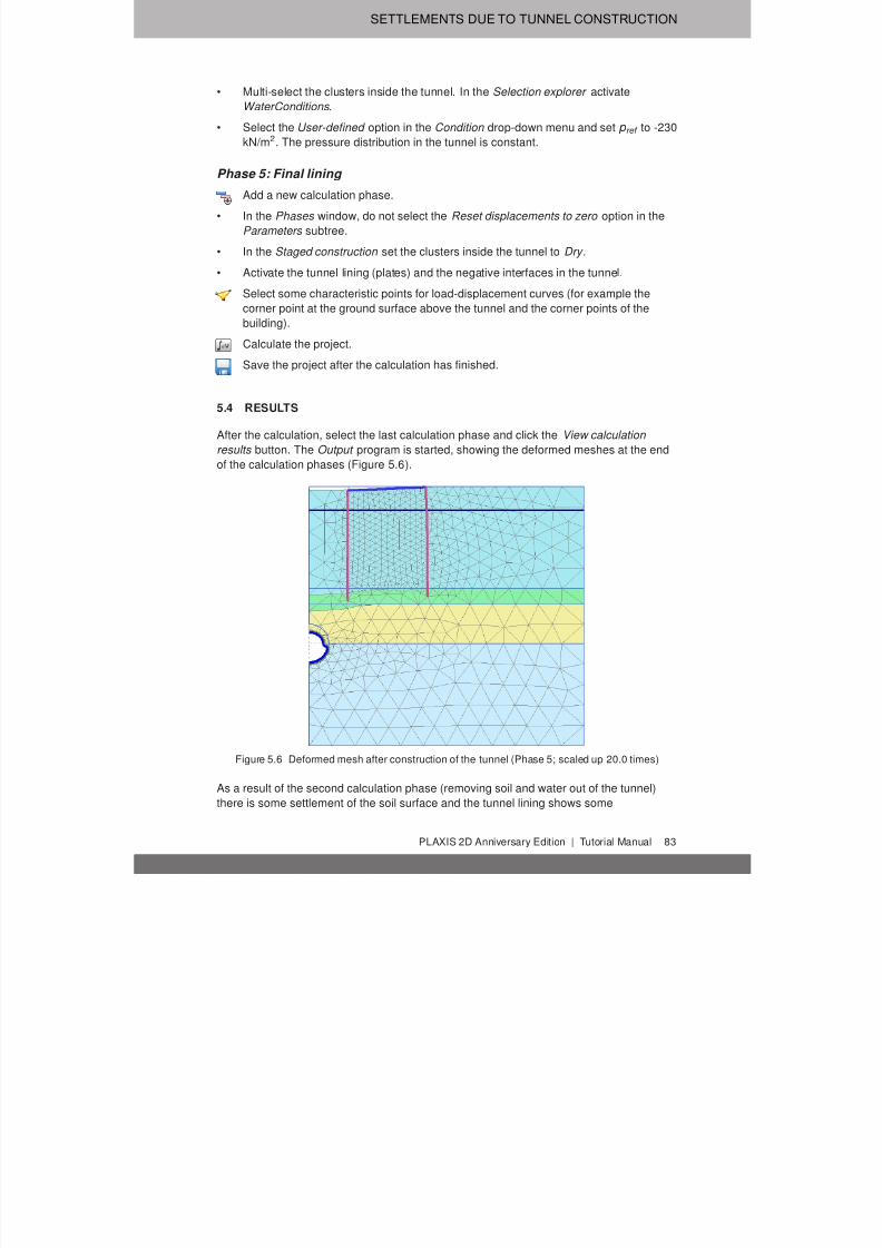
7/21/2019 2DAnniversaryEdition 1 Tutorial
http://slidepdf.com/reader/full/2danniversaryedition-1-tutorial 83/176
SETTLEMENTS DUE TO TUNNEL CONSTRUCTION
• Multi-select the clusters inside the tunnel. In the Selection explorer activate
WaterConditions .
• Select the User-defined option in the Condition drop-down menu and set p ref to -230
kN/m2. The pressure distribution in the tunnel is constant.
Phase 5: Final lining
Add a new calculation phase.
• In the Phases window, do not select the Reset displacements to zero option in the
Parameters subtree.
• In the Staged construction set the clusters inside the tunnel to Dry .
• Activate the tunnel lining (plates) and the negative interfaces in the tunnel.
Select some characteristic points for load-displacement curves (for example the
corner point at the ground surface above the tunnel and the corner points of thebuilding).
Calculate the project.
Save the project after the calculation has finished.
5.4 RESULTS
After the calculation, select the last calculation phase and click the View calculation
results button. The Output program is started, showing the deformed meshes at the end
of the calculation phases (Figure 5.6).
Figure 5.6 Deformed mesh after construction of the tunnel (Phase 5; scaled up 20.0 times)
As a result of the second calculation phase (removing soil and water out of the tunnel)
there is some settlement of the soil surface and the tunnel lining shows some
PLAXIS 2D Anniversary Edition | Tutorial Manual 83

7/21/2019 2DAnniversaryEdition 1 Tutorial
http://slidepdf.com/reader/full/2danniversaryedition-1-tutorial 84/176
TUTORIAL MANUAL
deformation. In this phase the axial force in the lining is the maximum axial force that will
be reached. The lining forces can be viewed by double clicking the lining and selecting
force related options from the Force menu. The plots of the axial forces and bending
moment are scaled by factors of 5·10-3 and 0.02 respectively (Figure 5.7).
Figure 5.7 Axial forces and Bending moments in the lining after the second phase
The plot of effective stresses, Figure 5.8, shows that arching occurs around the tunnel.
This arching reduces the stresses acting on the tunnel lining. As a result, the axial force
in the final phase is lower than that after the second calculation phase.
Figure 5.8 Effective principal stresses after the construction of the tunnel
84 Tutorial Manual | PLAXIS 2D Anniversary Edition

7/21/2019 2DAnniversaryEdition 1 Tutorial
http://slidepdf.com/reader/full/2danniversaryedition-1-tutorial 85/176
SETTLEMENTS DUE TO TUNNEL CONSTRUCTION
To display the tilt of the structure:
Click the Distance measurement in the side toolbar.
• Click the node located at the left corner of the structure (5.0 3.0).
• Click the node located at the right corner of the structure (15.0 3.0). The Distance measurement information window is displayed where the resulting tilt of the structure
is given (Figure 5.9).
Figure 5.9 Distance measurement information window
PLAXIS 2D Anniversary Edition | Tutorial Manual 85

7/21/2019 2DAnniversaryEdition 1 Tutorial
http://slidepdf.com/reader/full/2danniversaryedition-1-tutorial 86/176
TUTORIAL MANUAL
86 Tutorial Manual | PLAXIS 2D Anniversary Edition
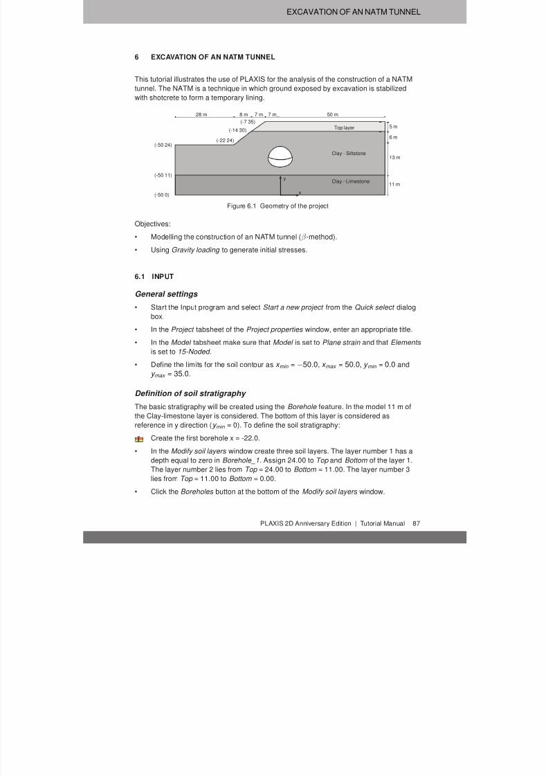
7/21/2019 2DAnniversaryEdition 1 Tutorial
http://slidepdf.com/reader/full/2danniversaryedition-1-tutorial 87/176
EXCAVATION OF AN NATM TUNNEL
6 EXCAVATION OF AN NATM TUNNEL
This tutorial illustrates the use of PLAXIS for the analysis of the construction of a NATM
tunnel. The NATM is a technique in which ground exposed by excavation is stabilized
with shotcrete to form a temporary lining.
x
y
28 m 8 m 7 m 7 m 50 m
5 m
6 m
13 m
11 m
Top layer
Clay - Siltstone
Clay - Limestone
(-50 0)
(-50 11)
(-50 24)(-22 24)
(-14 30)
(-7 35)
Figure 6.1 Geometry of the project
Objectives:
• Modelling the construction of an NATM tunnel (β -method).
• Using Gravity loading to generate initial stresses.
6.1 INPUT
General settings
• Start the Input program and select Start a new project from the Quick select dialog
box.
• In the Project tabsheet of the Project properties window, enter an appropriate title.
• In the Model tabsheet make sure that Model is set to Plane strain and that Elements
is set to 15-Noded .
• Define the limits for the soil contour as x min = −50.0, x max = 50.0, y min = 0.0 and
y max = 35.0.
Definition of soil stratigraphy
The basic stratigraphy will be created using the Borehole feature. In the model 11 m of
the Clay-limestone layer is considered. The bottom of this layer is considered as
reference in y direction (y min = 0). To define the soil stratigraphy:
Create the first borehole x = -22.0.
• In the Modify soil layers window create three soil layers. The layer number 1 has a
depth equal to zero in Borehole_1. Assign 24.00 to Top and Bottom of the layer 1.
The layer number 2 lies from Top = 24.00 to Bottom = 11.00. The layer number 3
lies from Top = 11.00 to Bottom = 0.00.
• Click the Boreholes button at the bottom of the Modify soil layers window.
PLAXIS 2D Anniversary Edition | Tutorial Manual 87

7/21/2019 2DAnniversaryEdition 1 Tutorial
http://slidepdf.com/reader/full/2danniversaryedition-1-tutorial 88/176
TUTORIAL MANUAL
• In the appearing menu select the Add option. The Add borehole window pops up.
• Specify the location of the second borehole (X = -14).
• Note that the soil layers are available for Borehole_2 . The layer number 1 has a
depth equal to zero in Borehole_2 . However as the depth of layer 2 is higher assign30.00 to Top and Bottom of the layer 1. The layer number 2 lies from Top = 30.00 to
Bottom = 11.00. The layer number 3 lies from Top = 11.00 to Bottom = 0.00.
• Create a new borehole (Borehole_3) at X = -7.
• In Borehole_3 the layer number 1 has a non-zero thicknesss and lies from Top =
35.00 to Bottom = 30.00. The layer number 2 lies from Top = 30.00 to Bottom =
11.00. The layer number 3 lies from Top = 11.00 to Bottom = 0.00.
• In all the boreholes the water level is located at y = 0 m.
• Specify the soil layer distribution as shown in Figure 6.2.
• Create soil material data sets according to Table 6.1 and assign them to the
corresponding layers (Figure 6.2).
• Close the Modify soil layers window and proceed to the Structures mode to define
the structural elements.
Table 6.1 Material properties of the soil layers
Parameter Name Top layer Clay-siltstone Clay-limestone Unit
General
Material model Model H ardening soil Hoek-Brown Hoek-Brown -
Type of material behaviour Type Drained Drained Drained -
Soil unit weight above phreatic level γ unsat 20 25 24 kN/m3
Soil unit weight below phreatic level γ sat 22 25 24 kN/m3
Initial void ratio e init 0.5 0.5 0.5 -
Parameters
Secant stiffness in standard drained triaxialtest
E ref 50 4.0·104 - - kN/m2
Tangent stiffness for primary oedometerloading
E ref oed 4.0·104 - - kN/m2
Unloading / reloading stiffness E ref ur 1.2·105 - - kN/m2
Power for stress-level dependency ofstiffness
m 0.5 - - -
Young's modulus E ' - 1.0·106 2.5·106 kN/m2
Poisson's ratio ν 'ur 0.2 0.25 0.25 -
Uniaxial compressive strength σci
- 2.5·104 5.0·104 kN/m2
Material constant for the intact rock m i - 4.0 10.0 -
Geological Strength Index GSI - 40.0 55.0 -
Disturbance factor D - 0.2 0.0 -
Cohesion c 'ref 10.0 - - kN/m2
Friction angle ϕ' 30 - - ◦
Dilatancy parameter ψmax - 30.0 35.0 ◦
Dilatancy parameter σψ - 400 1000 kN/m2
Interfaces
Interface strength − Rigid Manual Rigid -
Strength reduction factor R inter 1.0 0.5 1.0 -
88 Tutorial Manual | PLAXIS 2D Anniversary Edition

7/21/2019 2DAnniversaryEdition 1 Tutorial
http://slidepdf.com/reader/full/2danniversaryedition-1-tutorial 89/176
EXCAVATION OF AN NATM TUNNEL
Figure 6.2 Soil layer distribution
6.1.1 DEFINITION OF TUNNEL
In the Structures mode click the Create tunnel button in the side toolbar and click on
(0.0 16.0) in the draw area to specify the location of the tunnel. The Tunnel designer
window pops up.
• The default shape option (Free ) will be used. The default values of the rest of the
parameters defining the location of the tunnel in the model are valid as well.
• Click on the Segments tab.
Click the Add button in the side toolbar.
• In the segment info box set the Segment type to Arc . Set Radius to 10.4 m and the
Segment angle to 22◦. The default values of the remaining parameters are valid.
Add a new arc segment. Set Radius to 2.4 m and the Segment angle to 47◦. The
default values of the remaining parameters are valid.
Add a new arc segment. Set Radius to 5.8 m and the Segment angle to 50◦. The
default values of the remaining parameters are valid.
Click the Extend to symmetry axis option to complete the right half of the tunnel. Anew arc segment is automatically added closing the half of the tunnel.
Click the Symmetric close button to complete the tunnel. Four new arc segment are
automatically added closing the tunnel.
• Click on the Subsections tab.
Add a new subsection. This subsection will be used to separate the top heading
(upper excavation cluster) from the invert (lower excavation cluster).
• Set Offset 2 to 3 m. Select the Arc option from the Segment type drop-down menu.
Set Radius to 11 m and Segment angle to 360 ◦.
PLAXIS 2D Anniversary Edition | Tutorial Manual 89

7/21/2019 2DAnniversaryEdition 1 Tutorial
http://slidepdf.com/reader/full/2danniversaryedition-1-tutorial 90/176
TUTORIAL MANUAL
Figure 6.3 Segments in the tunnel cross section
Select all the geometric entities in the slice.
Click the Intersect button.
Delete the part of the subsection outside of the slice by selecting it in the display
area and clicking the Delete button in the side toolbar.
• Proceed to the Properties mode.
• Multi-select the polycurves in the display area and select the Create plate option in
the appearing menu.
• Click <Ctrl> + <M> to create a new material dataset according to Table 6.2.
• Multi-select the polycurves in the display area and right click and assign the Lining
material dataset to all the plates in the tunnel.
Table 6.2 Material properties of the plates
Parameter Name Lining Unit
Material type Type Elastic; Isotropic kN/m
Normal stiffness EA 6.0·106 kN/m
Flexural rigidity EI 2.0·104 kNm2 /m
Weight w 5.0 kN/m/m
Poisson's ratio ν 0.15 -
• Assign negative interfaces to the lines defining the shape of the tunnel (not the
excavation levels). The final tunnel view in the Tunnel designer window is given in
Figure 6.4.
• Click on Generate to update the tunnel in the model and press Close .
90 Tutorial Manual | PLAXIS 2D Anniversary Edition

7/21/2019 2DAnniversaryEdition 1 Tutorial
http://slidepdf.com/reader/full/2danniversaryedition-1-tutorial 91/176
EXCAVATION OF AN NATM TUNNEL
Figure 6.4 Final tunnel
6.2 MESH GENERATION
The default global coarseness parameter (Medium ) can be accepted in this case.
• Proceed to the Mesh mode.
Create the mesh. Use the default option for the Element distribution parameter
(Medium ).
View the mesh. The generated mesh is shown in Figure 6.5.
• Click on the Close tab to close the Output program.
Figure 6.5 The generated mesh
6.3 CALCULATIONS
To simulate the construction of the tunnel it is clear that a staged construction calculationis needed.
• Click on the Staged construction tab to proceed with the definition of the calculation
PLAXIS 2D Anniversary Edition | Tutorial Manual 91
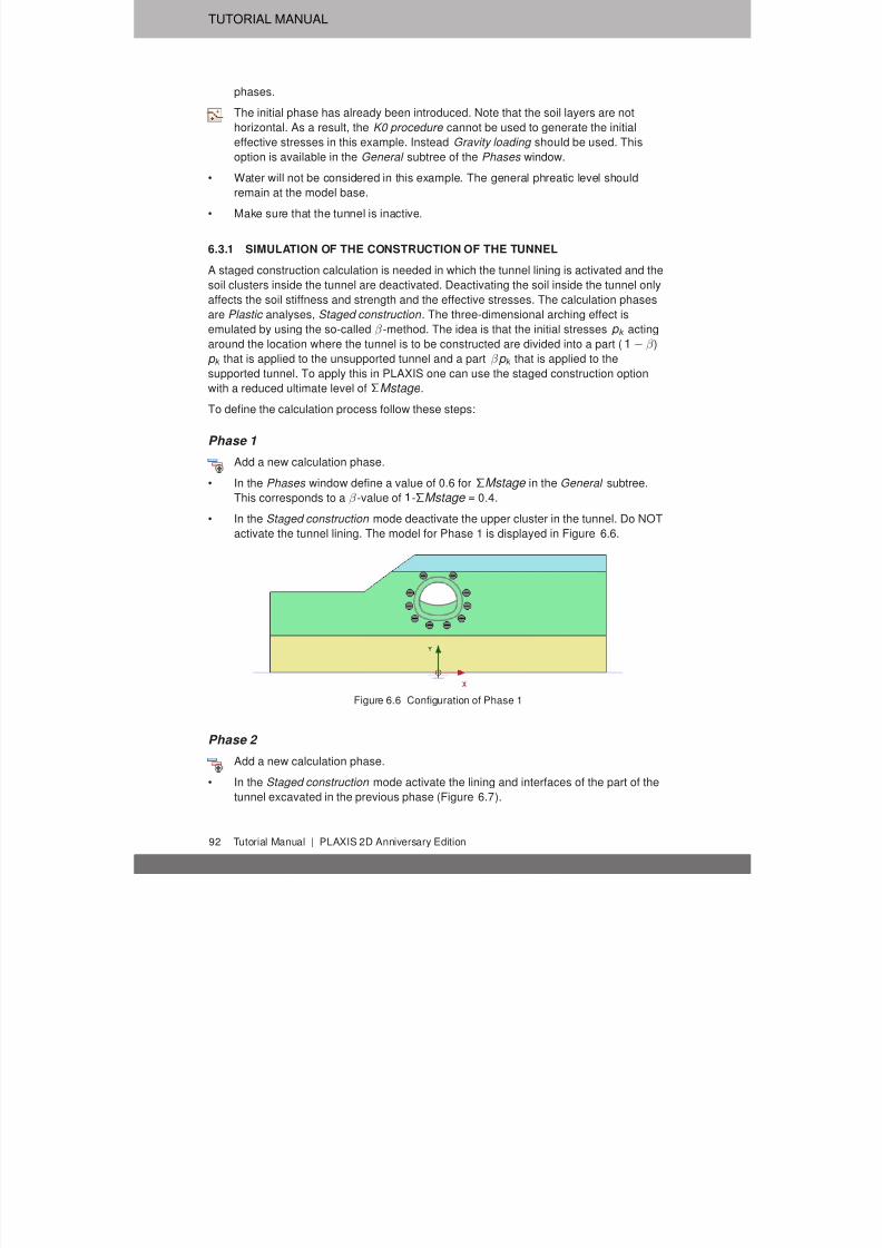
7/21/2019 2DAnniversaryEdition 1 Tutorial
http://slidepdf.com/reader/full/2danniversaryedition-1-tutorial 92/176
TUTORIAL MANUAL
phases.
The initial phase has already been introduced. Note that the soil layers are not
horizontal. As a result, the K0 procedure cannot be used to generate the initial
effective stresses in this example. Instead Gravity loading should be used. This
option is available in the General subtree of the Phases window.
• Water will not be considered in this example. The general phreatic level should
remain at the model base.
• Make sure that the tunnel is inactive.
6.3.1 SIMULATION OF THE CONSTRUCTION OF THE TUNNEL
A staged construction calculation is needed in which the tunnel lining is activated and the
soil clusters inside the tunnel are deactivated. Deactivating the soil inside the tunnel only
affects the soil stiffness and strength and the effective stresses. The calculation phases
are Plastic analyses, Staged construction . The three-dimensional arching effect is
emulated by using the so-called β -method. The idea is that the initial stresses p k acting
around the location where the tunnel is to be constructed are divided into a part (1 − β )
p k that is applied to the unsupported tunnel and a part β p k that is applied to the
supported tunnel. To apply this in PLAXIS one can use the staged construction option
with a reduced ultimate level of ΣMstage .
To define the calculation process follow these steps:
Phase 1
Add a new calculation phase.
• In the Phases window define a value of 0.6 for ΣMstage in the General subtree.
This corresponds to a β -value of 1-ΣMstage = 0.4.
• In the Staged construction mode deactivate the upper cluster in the tunnel. Do NOT
activate the tunnel lining. The model for Phase 1 is displayed in Figure 6.6.
Figure 6.6 Configuration of Phase 1
Phase 2
Add a new calculation phase.
• In the Staged construction mode activate the lining and interfaces of the part of the
tunnel excavated in the previous phase (Figure 6.7).
92 Tutorial Manual | PLAXIS 2D Anniversary Edition

7/21/2019 2DAnniversaryEdition 1 Tutorial
http://slidepdf.com/reader/full/2danniversaryedition-1-tutorial 93/176
EXCAVATION OF AN NATM TUNNEL
• Note that the value of ΣMstage is automatically reset to 1.0.
Figure 6.7 Configuration of Phase 2
Phase 3
Add a new calculation phase.
• In the Phases window define a value of 0.6 for ΣMstage in the General subtree.
This corresponds to a β -value of 1-ΣMstage = 0.4.
• In the Staged construction mode deactivate the lower cluster (invert) and the
temporary lining in the middle of the tunnel (Figure 6.8).
Figure 6.8 Configuration of Phase 3
Phase 4
Add a new calculation phase.
• Activate the remaining lining and interfaces. All the plates and interfaces around the
full tunnel are active (Figure 6.9).
• Note that the value of ΣMstage is automatically reset to 1.0.
Select a node at the slope crest point and the tunnel crest. These points might be of
interest to evaluate the deformation during the construction phases.
Calculate the project.
Save the project after the calculation has finished.
PLAXIS 2D Anniversary Edition | Tutorial Manual 93

7/21/2019 2DAnniversaryEdition 1 Tutorial
http://slidepdf.com/reader/full/2danniversaryedition-1-tutorial 94/176
TUTORIAL MANUAL
Figure 6.9 Configuration of Phase 4
6.4 RESULTS
After the calculation, select the last calculation phase and click the View calculation
results button. The Output program is started, showing the deformed mesh at the end of
the calculation phases (Figure 6.10).
Figure 6.10 The deformed mesh at the end of the the final calculation phase
To display the bending moments resulting in the tunnel:
To select the lining of all the tunnel sections, click the corresponding button in the
side toolbar and drag the mouse to define a rectangle where all the tunnel sections
are included. Select the Plate option in the appearing window (Figure 6.11) and
press View . Note that the tunnel lining is displayed in the Structures view.
Figure 6.11 Select structures window
• From the Forces menu select the Bending moment M option. The result, scaled by a
factor or 0.5 is displayed in Figure 6.12.
94 Tutorial Manual | PLAXIS 2D Anniversary Edition

7/21/2019 2DAnniversaryEdition 1 Tutorial
http://slidepdf.com/reader/full/2danniversaryedition-1-tutorial 95/176
EXCAVATION OF AN NATM TUNNEL
Figure 6.12 Resulting bending moments in the NATM tunnel
PLAXIS 2D Anniversary Edition | Tutorial Manual 95

7/21/2019 2DAnniversaryEdition 1 Tutorial
http://slidepdf.com/reader/full/2danniversaryedition-1-tutorial 96/176
TUTORIAL MANUAL
96 Tutorial Manual | PLAXIS 2D Anniversary Edition
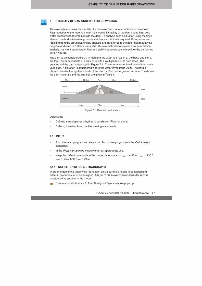
7/21/2019 2DAnniversaryEdition 1 Tutorial
http://slidepdf.com/reader/full/2danniversaryedition-1-tutorial 97/176
STABILITY OF DAM UNDER RAPID DRAWDOWN
7 STABILITY OF DAM UNDER RAPID DRAWDOWN
This example concerns the stability of a reservoir dam under conditions of drawdown.
Fast reduction of the reservoir level may lead to instability of the dam due to high pore
water pressures that remain inside the dam. To analyse such a situation using the finiteelement method, a transient groundwater flow calculation is required. Pore pressures
resulting from the groundwater flow analysis are transferred to the deformation analysis
program and used in a stability analysis. This example demonstrates how deformation
analysis, transient groundwater flow and stability analysis can interactively be performed
in PLAXIS 2D.
The dam to be considered is 30 m high and the width is 172.5 m at the base and 5 m at
the top. The dam consists of a clay core with a well graded fill at both sides. The
geometry of the dam is depicted in Figure 7.1. The normal water level behind the dam is
25 m high. A situation is considered where the water level drops 20 m. The normal
phreatic level at the right hand side of the dam is 10 m below ground surface. The data ofthe dam materials and the sub-soil are given in Table 1.
x
y
50 m 77.5 m
5 m
5 m
25 m
20 m 120 m120 m
37.5 m
30 m
30 m
90 m
Core
FillFill
Subsoil
Figure 7.1 Geometry of the dam
Objectives:
• Defining time-dependent hydraulic conditions (Flow functions)
• Defining transient flow conditions using water levels
7.1 INPUT
• Start the Input program and select the Start a new project from the Quick select
dialog box.
• In the Project properties window enter an appropriate title.
• Keep the default units and set the model dimensions to x min = -130.0, x max = 130.0,
y min = -30.0 and y max = 30.0.
7.1.1 DEFINITION OF SOIL STRATIGRAPHY
In order to define the underlying foundation soil, a borehole needs to be added and
material properties must be assigned. A layer of 30 m overconsolidated silty sand isconsidered as sub-soil in the model.
Create a borehole at x = 0. The Modify soil layers window pops up.
PLAXIS 2D Anniversary Edition | Tutorial Manual 97

7/21/2019 2DAnniversaryEdition 1 Tutorial
http://slidepdf.com/reader/full/2danniversaryedition-1-tutorial 98/176
TUTORIAL MANUAL
• Add a soil layer extending from ground surface (y = 0.0) to a depth of 30 m (y =
-30.0).
Open the Material sets window.
• Create data sets under Soil and interfaces set type according to the informationgiven in Table 7.1. Note that the Interfaces and Initial tabsheets are not relevant (no
interfaces or K0 procedure used).
• Assign the Subsoil material dataset to the soil layer in the borehole.
Table 7.1 Material properties of the dam and sub-soil
Parameter Name Core Fill Subsoil Unit
General
Material model Model Mohr-Coulomb Mohr-Coulomb Mohr-Coulomb -
Drainage type Type Undrained (B) Drained Drained -
Soil unit weight above p.l. γ unsat 16.0 16.0 17.0 kN/m3
Soil unit weight below p.l. γ sat
18.0 20.0 21.0 kN/m3
Parameters
Young's modulus E ' 1.5·103 2.0·104 5.0·104 kN/m2
Poisson's ratio ν ' 0.35 0.33 0.3 -
Cohesion c 'ref - 5.0 1.0 kN/m2
Undrained shear strength s u ,ref 5.0 - - kN/m2
Friction angle ϕ' - 31 35.0 ◦
Dilatancy angle ψ - 1.0 5.0 ◦
Young's modulus inc. E 'inc 300 - - kN/m2
Reference level y ref 30 - - m
Undrained shear strength inc. s u ,inc 3.0 - - kN/m2
Reference level y ref 30 - - m
FlowFlow data set Model Hypres Hypres Hypres -
Model - VanGenuchten
VanGenuchten
VanGenuchten
-
Soil - Subsoil Subsoil Subsoil -
Soil coarseness - Very fine Coarse Coarse -
Horizontal permeability k x 1.0·10-4 1.00 0.01 m/day
Vertical permeability k y 1.0·10-4 1.00 0.01 m/day
7.1.2 DEFINITION OF THE EMBANKMENT
The embankment will be defined in the Structures mode.
Define a polygon by specifying points located at (-80.0 0.0), (92.5 0.0), (2.5 30.0)
and (-2.5 30.0).
To create the sub-clusters in the embankment define two cutting lines from (-10.0
0.0) to (-2.5 30.0) and from (10.0 0.0) to (2.5 30.0).
• Assign the corresponding material datasets to the soil clusters.
7.2 MESH GENERATION
• Proceed to the Mesh mode.Create the mesh. Use the Fine option for the Element distribution parameter.
View the generated mesh. The generated mesh is shown in Figure 7.2.
98 Tutorial Manual | PLAXIS 2D Anniversary Edition
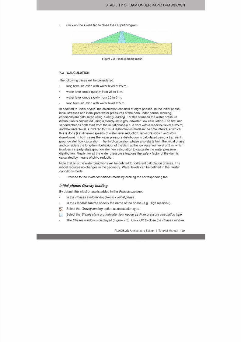
7/21/2019 2DAnniversaryEdition 1 Tutorial
http://slidepdf.com/reader/full/2danniversaryedition-1-tutorial 99/176
STABILITY OF DAM UNDER RAPID DRAWDOWN
• Click on the Close tab to close the Output program.
Figure 7.2 Finite element mesh
7.3 CALCULATION
The following cases will be considered:
• long term situation with water level at 25 m.
• water level drops quickly from 25 to 5 m.
• water level drops slowly from 25 to 5 m.
• long term situation with water level at 5 m.
In addition to Initial phase , the calculation consists of eight phases. In the initial phase,
initial stresses and initial pore water pressures of the dam under normal working
conditions are calculated using Gravity loading . For this situation the water pressure
distribution is calculated using a steady-state groundwater flow calculation. The first and
second phases both start from the initial phase (i.e. a dam with a reservoir level at 25 m)and the water level is lowered to 5 m. A distinction is made in the time interval at which
this is done (i.e. different speeds of water level reduction; rapid drawdown and slow
drawdown). In both cases the water pressure distribution is calculated using a transient
groundwater flow calculation. The third calculation phase also starts from the initial phase
and considers the long-term behaviour of the dam at the low reservoir level of 5 m, which
involves a steady-state groundwater flow calculation to calculate the water pressure
distribution. Finally, for all the water pressure situations the safety factor of the dam is
calculated by means of phi-c reduction.
Note that only the water conditions will be defined for different calculation phases. The
model requires no changes in the geometry. Water levels can be defined in the Water conditions mode.
• Proceed to the Water conditions mode by clicking the corresponding tab.
Initial phase: Gravity loading
By default the initial phase is added in the Phases explorer .
• In the Phases explorer double-click Initial phase .
• In the General subtree specify the name of the phase (e.g. High reservoir).
Select the Gravity loading option as calculation type.
Select the Steady state groundwater flow option as Pore pressure calculation type
• The Phases window is displayed (Figure 7.3). Click OK to close the Phases window.
PLAXIS 2D Anniversary Edition | Tutorial Manual 99

7/21/2019 2DAnniversaryEdition 1 Tutorial
http://slidepdf.com/reader/full/2danniversaryedition-1-tutorial 100/176
TUTORIAL MANUAL
Figure 7.3 The Phases window
Hint: Note that by default Undrained behaviour (A) and (B) are ignored for a
Gravity loading calculation type. The corresponding option is available in the
Deformation control parameters subtree in the Phases window.
Define the water level corresponding to the level of water in the reservoir prior to the
drawdown. The water level consists of four points; starting at the very left side at alevel of 25 m above the ground surface (-132.0 25.0); the second point is just inside
the dam at a level of 25 m (-10.0 25.0); the third point is near the dam toe (93.0
-10.0) and the forth point just outside the right boundary at a level of 10 m below the
ground surface (132.0 -10.0). The defined water level is shown in Figure 7.4.
• Right-click the created water level and select the Make global option in the
appearing menu. Note that the global water level can also be specified by selecting
the corresponding option in the GlobalWaterLevel menu in the Water subtree in the
Model conditions .
Hint: Straight lines can be defined by keeping the <Shift> key pressed while
defining the geometry.
Figure 7.4 High water level in the reservoir
100 Tutorial Manual | PLAXIS 2D Anniversary Edition

7/21/2019 2DAnniversaryEdition 1 Tutorial
http://slidepdf.com/reader/full/2danniversaryedition-1-tutorial 101/176
STABILITY OF DAM UNDER RAPID DRAWDOWN
• In the Model explorer expand the Attributes library .
• Expand the Water levels subtree. The levels created in the Water conditions mode
are grouped under User water levels .
• Expand the User water levels subtree. The created water level can be seen namedas 'UserWaterLevel_1'. The location of the water levels in Model explorer is shown
in Figure 7.5.
Figure 7.5 Water levels in Model explorer
• Double-click on the created water level and rename it as 'FullReservoir_Steady'.
This is a distinctive name that satisfies the naming requirements (no invalid
characters).
• Expand the Model conditions subtree.
• Expand the GroundWaterFlow subtree. Note that by default the boundary at the
bottom of the model is set to Closed . This is relevant for this example (Figure 7.6).
Figure 7.6 GroundwaterFlow boundary conditions in Model explorer
PLAXIS 2D Anniversary Edition | Tutorial Manual 101

7/21/2019 2DAnniversaryEdition 1 Tutorial
http://slidepdf.com/reader/full/2danniversaryedition-1-tutorial 102/176
TUTORIAL MANUAL
Phase 1: Rapid drawdown
In this phase rapid drawdown of the reservoir level is considered.
Add a new calculation phase.
• In Phases explorer double-click the newly added phase. The Phases window isdisplayed.
• In the General subtree specify the name of the phase (e.g. Rapid drawdown). Note
that the High reservoir phase is automatically selected in the Start from phase
drop-down menu.
Select the Fully coupled flow-deformation option as calculation type.
• Assign a value of 5 days to the Time interval parameter.
• Make sure that the Reset displacements to zero and Reset small strain options are
selected in the Deformation control parameters subtree.
• Click OK to close the Phases window.
• Due to the global nature of the water levels, if an attribute is assigned to a water
level in the model it will affect it in all phases. The water level in this phase has the
same geometry with the one previously defined, however it is time dependent and a
function needs to be assigned to it. As a result, it is required to create a new water
level with the same geometry and different attributes. In Model explorer right-click
on FullReservoir_Steady and select the Duplicate option in the appearing menu
(Figure 7.7). A copy of the water level is created.
Figure 7.7 Copying water levels in Model explorer
• Rename the newly created water level as 'FullReservoir_Rapid'.
The behaviour of the water levels can be described by specifying Flow functions . Notethat Flow functions are global entities and are available under the Attributes library in
Model explorer . To define the flow functions:
102 Tutorial Manual | PLAXIS 2D Anniversary Edition

7/21/2019 2DAnniversaryEdition 1 Tutorial
http://slidepdf.com/reader/full/2danniversaryedition-1-tutorial 103/176
STABILITY OF DAM UNDER RAPID DRAWDOWN
• Right-click the Flow functions option in the Attributes library in the Model explorer
and select the Edit option in the appearing menu. The Flow functions window is
displayed.
In the Head functions tabsheet add a new function by clicking the corresponding
button. The new function is highlighted in the list and options to define the functionare displayed.
• Specify a proper name to the function for the rapid drawdown (e.g. Rapid).
• Select the Linear option from the Signal drop-down menu.
• Specify a time interval of 5 days.
• Assign a value of -20 m to ∆Head , representing the amount of the head decrease.
A graph is displayed showing the defined function (Figure 7.8).
Figure 7.8 The flow function for the rapid drawdown case
• Click OK to close the Flow functions window.
• In the Model explorer right-click on FullReservoir_Rapid and select the Use as
global phreatic level option in the appearing menu.
• Expand the FullReservoir_Rapid subtree. Note that the water level is composed of 3
water segments. Select the water segment in the upstream shoulder (left from the
dam, at the reservoir side).
• Expand the subtree of the selected segment and select the Time dependent option
for the TimeDependency parameter.
• Select the Rapid option for the HeadFunction parameter. Figure 7.9 shows the
selected water segment in Model explorer .
• In the Water subtree under the Model conditions in the Model explorer note that the
new water level (FullReservoir_Rapid) is assigned to GlobalWaterLevel .
PLAXIS 2D Anniversary Edition | Tutorial Manual 103
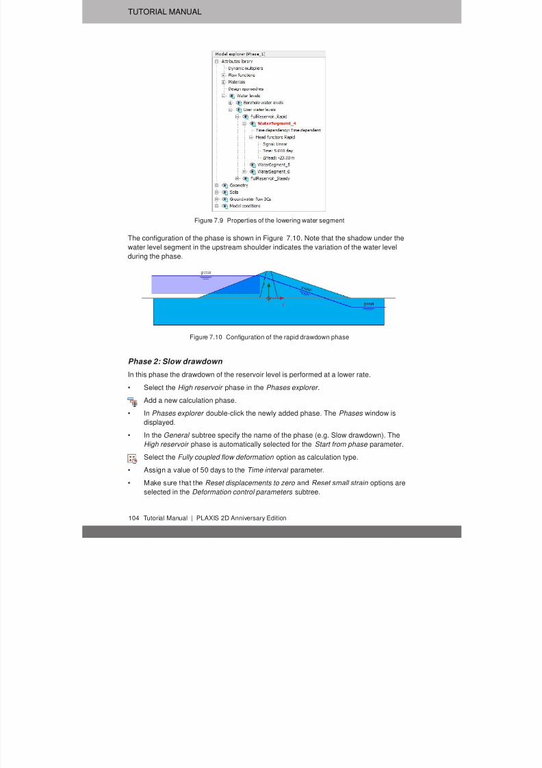
7/21/2019 2DAnniversaryEdition 1 Tutorial
http://slidepdf.com/reader/full/2danniversaryedition-1-tutorial 104/176
TUTORIAL MANUAL
Figure 7.9 Properties of the lowering water segment
The configuration of the phase is shown in Figure 7.10. Note that the shadow under the
water level segment in the upstream shoulder indicates the variation of the water level
during the phase.
Figure 7.10 Configuration of the rapid drawdown phase
Phase 2: Slow drawdown
In this phase the drawdown of the reservoir level is performed at a lower rate.
• Select the High reservoir phase in the Phases explorer .
Add a new calculation phase.
• In Phases explorer double-click the newly added phase. The Phases window is
displayed.
• In the General subtree specify the name of the phase (e.g. Slow drawdown). The
High reservoir phase is automatically selected for the Start from phase parameter.
Select the Fully coupled flow deformation option as calculation type.
• Assign a value of 50 days to the Time interval parameter.• Make sure that the Reset displacements to zero and Reset small strain options are
selected in the Deformation control parameters subtree.
104 Tutorial Manual | PLAXIS 2D Anniversary Edition

7/21/2019 2DAnniversaryEdition 1 Tutorial
http://slidepdf.com/reader/full/2danniversaryedition-1-tutorial 105/176
STABILITY OF DAM UNDER RAPID DRAWDOWN
• Click OK to close the Phases window.
• Create a new duplicate of the high water level. The newly created water level will be
used as Global water level in the slow drawdown phase. Even though the water
level in this phase has the same geometry as the previously defined ones, the flow
function for the time dependency is different.
• Rename the newly created water level as 'FullReservoir_Slow'.
Add a new flow function following the steps described for the previous phase.
• Specify a proper name to the function for the slow drawdown (e.g. Slow).
• Select the Linear option from the Signal drop-down menu.
• Specify a time interval of 50 days.
• Assign a value of -20 m to ∆Head , representing the amount of the head decrease.
A graph is displayed showing the defined function (Figure 7.11).
• Click OK to close the Flow functions window.
Figure 7.11 The flow function for the slow drawdown case
• In the Model explorer right-click on FullReservoir_Slow and select the Use as global
phreatic level option in the appearing menu.
• Expand the FullReservoir_Slow subtree. Select the water segment in the upstream
shoulder (left from the dam, at the reservoir side). The segment selected in Model
explorer is indicated by a red colour in the model.
• Expand the subtree of the selected segment and select the Time dependent option
for the TimeDependency parameter.
• Select the Slow option for the HeadFunction parameter.
• In the Water subtree under the Model conditions in the Model explorer note that the
PLAXIS 2D Anniversary Edition | Tutorial Manual 105
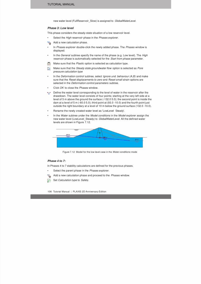
7/21/2019 2DAnniversaryEdition 1 Tutorial
http://slidepdf.com/reader/full/2danniversaryedition-1-tutorial 106/176
TUTORIAL MANUAL
new water level (FullReservoir_Slow) is assigned to GlobalWaterLevel .
Phase 3: Low level
This phase considers the steady-state situation of a low reservoir level.
• Select the High reservoir phase in the Phases explorer .
Add a new calculation phase.
• In Phases explorer double-click the newly added phase. The Phases window is
displayed.
• In the General subtree specify the name of the phase (e.g. Low level). The High
reservoir phase is automatically selected for the Start from phase parameter.
Make sure that the Plastic option is selected as calculation type.
Make sure that the Steady state groundwater flow option is selected as Pore
pressure calculation type
• In the Deformation control subtree, select Ignore und. behaviour (A,B) and make
sure that the Reset displacements to zero and Reset small strain options are
selected in the Deformation control parameters subtree.
• Click OK to close the Phases window.
Define the water level corresponding to the level of water in the reservoir after the
drawdown. The water level consists of four points; starting at the very left side at a
level of 5 m above the ground the surface (-132.0 5.0); the second point is inside the
dam at a level of 5 m (-60.0 5.0); third point at (93.0 -10.0) and the fourth point just
outside the right boundary at a level of 10 m below the ground surface (132.0 -10.0).
• Rename the newly created water level as 'LowLevel_Steady'.
• In the Water subtree under the Model conditions in the Model explorer assign the
new water level (LowLevel_Steady) to GlobalWaterLevel . All the defined water
levels are shown in Figure 7.12.
Figure 7.12 Model for the low level case in the Water conditions mode
Phase 4 to 7:
In Phases 4 to 7 stability calculations are defined for the previous phases.
• Select the parent phase in the Phases explorer .
Add a new calculation phase and proceed to the Phases window.
Set Calculation type to Safety .
106 Tutorial Manual | PLAXIS 2D Anniversary Edition

7/21/2019 2DAnniversaryEdition 1 Tutorial
http://slidepdf.com/reader/full/2danniversaryedition-1-tutorial 107/176
STABILITY OF DAM UNDER RAPID DRAWDOWN
• In the Deformation control subtree, select Reset displacements to zero .
• In the Numerical control parameters subtree set the Max steps parameter to 30 for
Phase 4 and to 50 for phases 5 to 7. The final view of Phases explorer is given in
Figure 7.13.
Figure 7.13 The final view of Phases explorer
• Proceed to the Staged construction mode.
Select nodes located at the crest (-2.5 30.0) and at the toe of the dam (-80.0 0.0).
Start the calculation process by clicking the Calculate button in the Staged
construction mode.
Save the project after the calculation has finished.
7.4 RESULTS
The results of the four groundwater flow calculations in terms of pore pressure distribution
are shown in Figures 7.14 to 7.17. Four different situations were considered:
• The steady-state situation with a high (standard) reservoir level (Figure 7.14).
Figure 7.14 Pore pressure distribution, (p active ), for high reservoir level
• The pore pressure distribution after rapid drawdown of the reservoir level (Figure
7.15).
PLAXIS 2D Anniversary Edition | Tutorial Manual 107

7/21/2019 2DAnniversaryEdition 1 Tutorial
http://slidepdf.com/reader/full/2danniversaryedition-1-tutorial 108/176
TUTORIAL MANUAL
Figure 7.15 Pore pressure distribution, (p active ), after rapid drawdown
• The pore pressure distribution after slow drawdown of the reservoir level (Figure
7.16).
Figure 7.16 Pore pressure distribution, (p active ), after slow drawdown
• The steady-state situation with a low reservoir level (Figure 7.17).
Figure 7.17 Pore pressure distribution, (p active ), for low reservoir level
When the change of pore pressure is taken into account in a deformation analysis, some
additional deformation of the dam will occur. These deformations and the effective stress
distribution can be viewed on the basis of the results of the first four calculation phases.
Here, attention is focused on the variation of the safety factor of the dam for the different
situations. Therefore, the development of ΣMsf is plotted for the phases 4 to 7 as afunction of the displacement of the dam crest point (see Figure 7.18).
Rapid drawdown of a reservoir level can reduce the stability of a dam significantly. Fully
coupled flow-deformation and stability analysis can be performed with PLAXIS 2D to
effectively analyze such situations
108 Tutorial Manual | PLAXIS 2D Anniversary Edition

7/21/2019 2DAnniversaryEdition 1 Tutorial
http://slidepdf.com/reader/full/2danniversaryedition-1-tutorial 109/176
STABILITY OF DAM UNDER RAPID DRAWDOWN
Figure 7.18 Safety factors for different situations
PLAXIS 2D Anniversary Edition | Tutorial Manual 109

7/21/2019 2DAnniversaryEdition 1 Tutorial
http://slidepdf.com/reader/full/2danniversaryedition-1-tutorial 110/176
TUTORIAL MANUAL
110 Tutorial Manual | PLAXIS 2D Anniversary Edition

7/21/2019 2DAnniversaryEdition 1 Tutorial
http://slidepdf.com/reader/full/2danniversaryedition-1-tutorial 111/176
DRY EXCAVATION USING A TIE BACK WALL - ULS
8 DRY EXCAVATION USING A TIE BACK WALL - ULS
In this tutorial a Ultimate Limit State (ULS) calculation will be defined and performed for
the submerged construction of an excavation. The geometry model of Chapter 3 will be
used. The Design approaches feature is introduced in this example. This feature allowsfor the use of partial factors for loads and model parameters after a serviceability
calculation has already been performed.
Objectives:
• Using Design approaches
8.1 INPUT
In order to define a design approach:
• Open the project created in Chapter 3 and save it under a different name.
• Select the Design approaches option in the Soil or Structures menu. The
corresponding window is displayed.
• Click the Add button. A new design approach is added in the list.
• In this example the design approach 3 of the Eurocode 7 will be used. This design
approach involves partial factors for loads and partial factors for materials (strength).
Click the design approach in the list and specify a representative name (ex:
'Eurocode 7 - DA 3').
• In the lower part of the window the partial factors can be defined for loads andmaterials. Set the partial factor for Variable unfavourable 1.3.
Figure 8.1 Partial factors for loads
• Click the Materials tab.
• Assign a value of 1.25 to Effective friction angle and Effective cohesion .
PLAXIS 2D Anniversary Edition | Tutorial Manual 111

7/21/2019 2DAnniversaryEdition 1 Tutorial
http://slidepdf.com/reader/full/2danniversaryedition-1-tutorial 112/176
TUTORIAL MANUAL
Figure 8.2 Partial factors for materials
• Click the Materials button. The Material sets window pops up.
• Open the Loam material data set. Note that the view has changed. In the current
view it is possible to assign factors to different soil parameters, as well as to see the
effect of these factors on the soil parameters.
• Click the Parameters tab. In the Parameters tabsheet select the corresponding
labels for c 'ref and ϕ' (Figure 8.3)
• Do the same for the remaining soil data sets.
• Close the Design approaches window.
Figure 8.3 Assignment of partial factors to material parameters
112 Tutorial Manual | PLAXIS 2D Anniversary Edition

7/21/2019 2DAnniversaryEdition 1 Tutorial
http://slidepdf.com/reader/full/2danniversaryedition-1-tutorial 113/176
DRY EXCAVATION USING A TIE BACK WALL - ULS
Hint: Note that a partial factor for φ and ψ applies to the tangent of φ and ψ
respectively.
8.2 CALCULATIONS
There are two main schemes to perform design calculations in relation to serviceability
calculations (Section ?? of the Reference Manual). The first approach is used in this
tutorial.
• Proceed to the Staged construction mode.
• Click Phase_1 in the Phases explorer .
Add a new phase.• Double-click the newly added phase to open the Phases window.
• In the General subtree of the Phases window select the defined design approach in
the corresponding drop-down menu.
• In the Model explorer expand the Line loads and all the subtrees under it.
• Select the Variable unfavourable option in the LoadFactorLabel drop-down menu of
the static component of the load (Figure 8.4).
Figure 8.4 Assignment of factor label to loads in the Selection explorer
• Follow the same steps to define ULS phases for all the remaining SLS phases.Make sure that the Phase 7 starts from Phase 1, Phase 8 from Phase 2, Phase 9
from Phase 3 and so on.
PLAXIS 2D Anniversary Edition | Tutorial Manual 113

7/21/2019 2DAnniversaryEdition 1 Tutorial
http://slidepdf.com/reader/full/2danniversaryedition-1-tutorial 114/176
TUTORIAL MANUAL
Select some characteristic points for curves (for example the connection points of
the ground anchors on the diaphragm wall, such as (40.0 27.0) and (40.0 23.0)).
Calculate the project.
Save the project after the calculation has finished.
8.3 RESULTS
The results obtained for the design approach phases can be evaluated in Output. Figure
8.5 displays the ΣMstage - |u | plot for the node located at (40.0 27.0).
Figure 8.5 Σ− Mstage - |u | plot for the ULS phases
If the ULS calculations have successfully finished, the model complies with the
corresponding design approach. If there are doubts about this due to excessive
deformations, an additional Safety calculation may be considered using the same design
approach, which should then result in a stable ΣM sf value larger than 1.0. Note that if
partial factors have been used it is not necessary that ΣM sf also includes a safety margin.
Hence, in this case ΣMsf just larger that 1.0 is enough. Figure 8.6 displays the ΣMsf -
|u | plot for the Safety calculations of the Phase 6 and the corresponding ULS phase(Phase 12). It can be concluded that the situation complies with the design requirements.
114 Tutorial Manual | PLAXIS 2D Anniversary Edition

7/21/2019 2DAnniversaryEdition 1 Tutorial
http://slidepdf.com/reader/full/2danniversaryedition-1-tutorial 115/176
DRY EXCAVATION USING A TIE BACK WALL - ULS
Figure 8.6 ΣMsf - |u | plot for the last calculation phase and the corresponding ULS phase
PLAXIS 2D Anniversary Edition | Tutorial Manual 115

7/21/2019 2DAnniversaryEdition 1 Tutorial
http://slidepdf.com/reader/full/2danniversaryedition-1-tutorial 116/176
TUTORIAL MANUAL
116 Tutorial Manual | PLAXIS 2D Anniversary Edition

7/21/2019 2DAnniversaryEdition 1 Tutorial
http://slidepdf.com/reader/full/2danniversaryedition-1-tutorial 117/176
FLOW THROUGH AN EMBANKMENT
9 FLOW THROUGH AN EMBANKMENT
In this chapter the flow through an embankment will be considered. The crest of the
embankment has a width of 2.0 m. Initially the water in the river is 1.5 m deep. The
difference in water level between the river and the polder is 3.5 m.
Figure 9.1 shows the layout of the embankment problem where free surface groundwater
flow occurs. Flow takes place from the left side (river) to the right side (polder). As a
result seepage will take place at the right side of the embankment. The position of the
phreatic level depends on the river water level, which varies in time.
x
y
1 m
2 m2 m
3 m
3 m
3 m10 m
5 m
6 m
Figure 9.1 Geometry of the embankment
Objectives:
• Performing Groundwater flow only analysis
• Using cross section curves
9.1 INPUT
To create the geometry model, follow these steps:
General settings
• Start the Input program and select Start a new project from the Quick select dialog
box.
• In the Project tabsheet of the Project properties window, enter an appropriate title.
• In the Model tabsheet keep the default options for Model (Plane strain ), and
Elements (15-Node ).
• Keep the default values for units and the general parameters.
• Set the model dimensions to x min = 0.0 m, x max = 23.0 m, y min = 0.0 m, y max = 6.0 m
and press OK to close the Project properties window.
Definition of soil stratigraphy
To define the soil stratigraphy:
Create a borehole at x = 2. The Modify soil layers window pops up.
• Specify the head value as 4.5.
PLAXIS 2D Anniversary Edition | Tutorial Manual 117

7/21/2019 2DAnniversaryEdition 1 Tutorial
http://slidepdf.com/reader/full/2danniversaryedition-1-tutorial 118/176
TUTORIAL MANUAL
• Add a soil layer in the borehole. Set the top level to 3. No change is required for the
bottom boundary of the layer.
• Create the rest of the required boreholes according to the information given in Table
9.1.
Table 9.1 Information on the boreholes in the model
Borehole number Location (x) Head Top Bottom
1 2.0 4.5 3.0 0.0
2 8.0 4.5 6.0 0.0
3 10.0 4.0 6.0 0.0
4 20.0 1.0 1.0 0.0
Define the soil material according to the Table 9.2 and assign the material dataset to
the cluster. Skip the Interfaces and Initial tabsheets as these parameters are not
relevant.
Table 9.2 Properties of the embankment material (sand)
Parameter Name Sand Unit
General
Material model Model Linear elastic -
Type of material behaviour Type Drained -
Soil unit weight above phreatic
level
γ unsat 20 kN/m3
Soil unit weight below phreatic
level
γ sat 20 kN/m3
Parameters
Stiffness E ' 1.0· 104 kN/m2
Poisson's ratio ν ' 0.3 -
Flow parameters
Data set - Standard -
Soil type - Medium fine -
Set permeability to default - Yes -
Horizontal permeability k x 0.02272 m/day
Vertical permeability k y 0.02272 m/day
• After assigning the material to the soil cluster close the Modify soil layers window.
9.2 MESH GENERATION
• Proceed to the Mesh mode.
Refine the lines shown in Figure 9.2 by specifying a Coarseness factor of 0.5.
Click the Generate mesh button in order to generate the mesh. The Mesh options
window appears.
118 Tutorial Manual | PLAXIS 2D Anniversary Edition

7/21/2019 2DAnniversaryEdition 1 Tutorial
http://slidepdf.com/reader/full/2danniversaryedition-1-tutorial 119/176
FLOW THROUGH AN EMBANKMENT
Figure 9.2 Indication of the local refinement of the mesh in the model
• Select the Fine option in the Element distribution drop-down menu and generate the
mesh.
View the mesh. The resulting mesh is displayed in Figure 9.3).
• Click on the Close tab to close the Output program.
Figure 9.3 The generated mesh
9.3 CALCULATIONS
In this project only the flow related behaviour will be analysed. The calculation process
consists of three phases that will be defined in the Staged construction mode. In the
initial phase, the groundwater flow in steady state is calculated for an average river level.
In Phase 1, the transient groundwater flow is calculated for a harmonic variation of the
water level. In Phase 2, the calculation is similar as in Phase 1, but the period is longer.
• Click the Staged construction tab to proceed to the corresponding mode. A global
level is automatically created according to the head values specified for each
borehole (Table 9.1). The model in the Staged construction mode is shown in Figure
9.4.
Figure 9.4 The model in the Staged construction mode
PLAXIS 2D Anniversary Edition | Tutorial Manual 119

7/21/2019 2DAnniversaryEdition 1 Tutorial
http://slidepdf.com/reader/full/2danniversaryedition-1-tutorial 120/176
TUTORIAL MANUAL
Hint: Note that the 'internal' part of the global water level will be replaced by the
result of the groundwater flow calculation.
Initial phase:
• Double-click the initial phase in the Phases explorer.
• In the General subtree select the Groundwater flow only option as the Calculation
type .
• The default values of the remaining parameters are valid for this phase. Click OK to
close the Phases window.
• In the Model explorer expand the Model conditions subtree.
• In the Model conditions expand the GroundwaterFlow subtree. The default
boundary conditions (Figure 9.5) are relevant for the initial phase. Check that only
the bottom boundary is closed.
Figure 9.5 The groundwater flow boundary conditions for the initial phase
• In the Model explorer expand the Groundwater flow BCs subtree. The boundary
conditions at the extremities of the model are automatically created by the program
and listed under the GWFlowBaseBC .
Hint: Note that when the boundary conditions under the Groundwater flow BCs
subtree are active, the model conditions specified in the GrounwaterFlow are
ignored.
Phase 1:
Add a new calculation phase.
• In the Phases explorer double-click the current phase.
120 Tutorial Manual | PLAXIS 2D Anniversary Edition

7/21/2019 2DAnniversaryEdition 1 Tutorial
http://slidepdf.com/reader/full/2danniversaryedition-1-tutorial 121/176
FLOW THROUGH AN EMBANKMENT
• In the General subtree select the Transient groundwater flow option as pore
pressure calculation type.
• Set the Time interval to 1.0 day.
• In the Numerical control parameters subtree set the Max number of steps stored parameter to 50. The default values of the remaining parameters will be used.
• Click OK to close the Phases window.
Click the Select multiple objects button in the side toolbar.
Point to the Select lines option and click on the Select water boundaries option in
the appearing menu (Figure 9.6).
Figure 9.6 The Select water boundaries option in the Select multiple objects menu
• Select the hydraulic boundaries as shown in Figure 9.7.
• Right-click and select the Activate option in the appearing menu.
Figure 9.7 The time dependent boundaries in the model
• In the Selection explorer set the Behaviour parameter to Head .
• Set h ref to 4.5.
• Select the Time dependent option in the Time dependency drop-down menu.• Click on the Head function parameter.
Add a new head function.
• In the Flow functions window select the Harmonic option in the Signal drop-down
menu. Set the amplitude to 1.0 m, the phase angle to 0 ◦ and the period to 1.0 day
(Figure 9.8).
• Click OK to close the Flow functions window.
Phase 2:
Add a new calculation phase.
• In the Phases explorer double-click the current phase.
PLAXIS 2D Anniversary Edition | Tutorial Manual 121

7/21/2019 2DAnniversaryEdition 1 Tutorial
http://slidepdf.com/reader/full/2danniversaryedition-1-tutorial 122/176
TUTORIAL MANUAL
Figure 9.8 The flow function for the rapid case
• In the General subtree select the initial phase in the Start from phase drop-down
menu.
• Select the Transient groundwater flow option as pore pressure calculation type.
• Set the Time interval to 10.0 day.
• In the Numerical control parameters subtree set the Max number of steps stored parameter to 50. The default values of the remaining parameters will be used.
• Click OK to close the Phases window.
• In the Selection explorer click on the Head function parameter.
Add a new head function.
• In the Flow functions window select the Harmonic option in the Signal drop-down
menu. Set the amplitude to 1.0 m, the phase angle to 0 ◦ and the period to 10.0 day
(Figure 9.9).
• Click OK to close the Flow functions window.To select points to be considered in curves:
In the Staged construction mode click the Select point for curves button in the side
toolbar. The Connectivity plot is displayed in the Output program.
• In the Select points window select nodes located nearest to (0.0 3.0) and (8.0 2.5) to
be considered in curves.
• Click Update to close the output program.
Calculate the project.
Save the project after the calculation has finished.
122 Tutorial Manual | PLAXIS 2D Anniversary Edition

7/21/2019 2DAnniversaryEdition 1 Tutorial
http://slidepdf.com/reader/full/2danniversaryedition-1-tutorial 123/176
FLOW THROUGH AN EMBANKMENT
Figure 9.9 The flow function for the slow case
9.4 RESULTS
In the Output program the Create animation tool can be used to animate the results
displayed in the Output program. To create the animation follow these steps:
• In the Stresses menu select the Pore pressures → Groundwater head .
• Select the Create animation option in the File menu. The corresponding window
pops up.
• Define the name of the animation file and the location where it will be stored. By
default the program names it according to the project and stores it in the project
folder. In the same way animations can be created to compare the development of
pore pressures or flow field.
• Deselect the initial phase and Phase 2, such that only Phase 1 is included in the
animations and rename the animation accordingly. The Create animation window is
shown in Figure 9.10.
To view the results in a cross section:
Click the Cross section button in the side toolbar. The Cross section points window
pops up and the start and the end points of the cross section can be defined. Draw
a cross section through the points (2.0 3.0) and (20.0 1.0). The results in the cross
section are displayed in a new window.
• In the Cross section view select Pore pressures → p active in the Stresses menu.
• Select the Cross section curves option in the Tools menu. The Select steps for
curves window pops up.
• Select Phase 1. The variation of the results in the cross section is displayed in anew window.
• Do the same for Phase 2. This may take about 30 seconds,
PLAXIS 2D Anniversary Edition | Tutorial Manual 123

7/21/2019 2DAnniversaryEdition 1 Tutorial
http://slidepdf.com/reader/full/2danniversaryedition-1-tutorial 124/176
TUTORIAL MANUAL
Figure 9.10 Create animation window
• The variation of the results due to different time intervals in harmonic variation at a
specific cross section can be compared (Figure 9.11 and Figure 9.12).
It can be seen that the slower variation of the external water level has a more significant
influence on the pore pressures in the embankment and over a larger distance.
Figure 9.11 Active pore pressure variation in the cross section in Phase 1
124 Tutorial Manual | PLAXIS 2D Anniversary Edition

7/21/2019 2DAnniversaryEdition 1 Tutorial
http://slidepdf.com/reader/full/2danniversaryedition-1-tutorial 125/176
FLOW THROUGH AN EMBANKMENT
Figure 9.12 Active pore pressure variation in the cross section in Phase 2
PLAXIS 2D Anniversary Edition | Tutorial Manual 125

7/21/2019 2DAnniversaryEdition 1 Tutorial
http://slidepdf.com/reader/full/2danniversaryedition-1-tutorial 126/176
TUTORIAL MANUAL
126 Tutorial Manual | PLAXIS 2D Anniversary Edition

7/21/2019 2DAnniversaryEdition 1 Tutorial
http://slidepdf.com/reader/full/2danniversaryedition-1-tutorial 127/176
FLOW AROUND A SHEET PILE WALL
10 FLOW AROUND A SHEET PILE WALL
In this tutorial the flow around a sheetpile wall will be analyzed. The geometry model of
Chapter 3 will be used. The Well feature is introduced in this example.
Objectives:
• Using wells
10.1 INPUT
To create the geometry:
• Open the project defined in Chapter 3.
• Save the project under a different name (e.g. 'Flow around a sheet pile wall'). The
material parameters remain unchanged. The used flow parameters are shown inTable 10.1.
Table 10.1 Flow parameters
Parameter Name Silt Sand Loam Unit
Flow parameters
Data set - USDA USDA USDA -
Model - Van Genuchten Van Genuchten Van Genuchten -
Soil type - Silt Sand Loam -
> 2µm - 6.0 4.0 20.0 %
2µm − 50µm - 87.0 4.0 40.0 %
50µm − 2mm - 7.0 92.0 40.0 %
Set parameters to defaults - Yes Yes Yes -
Permeability in horizontal direction k x 0.5996 7.128 0.2497 m/day
Permeability in vertical direction k y 0.5996 7.128 0.2497 m/day
In the Structures mode click the Create hydraulic conditions button in the side
toolbar.
Select the Create well option in the appearing menu.
• Draw the first well by clicking on (42.0 23.0) and (42.0 20.0).
• Draw the second well by clicking on (58.0 23.0) and (58.0 20.0).
10.2 MESH GENERATION
• Proceed to the Mesh mode.
Create the mesh. Use the default option for the Element distribution parameter
(Medium ).
View the mesh. The resulting mesh is displayed in Figure 10.1.
• Click on the Close tab to close the Output program.
PLAXIS 2D Anniversary Edition | Tutorial Manual 127

7/21/2019 2DAnniversaryEdition 1 Tutorial
http://slidepdf.com/reader/full/2danniversaryedition-1-tutorial 128/176
TUTORIAL MANUAL
Figure 10.1 The generated mesh
10.3 CALCULATIONS
• Proceed to the Staged construction mode. In this project only groundwater flow
analysis will be performed.
In the Phases explorer remove the existing phases (Phases 1 to 6).
Initial phase
In this phase the initial steady-state pore pressure distribution is considered. To define
the initial phase:
• In the General subtree of the Phases window select the Groundwater flow only
option in the Calculation type drop-down menu.
• The standard settings for the remaining parameters are valid for this phase.
• The default groundwater flow boundary conditions are valid. Only the bottom
boundary of the model (BoundaryYMin ) is Closed whereas the rest of the
boundaries are Open .
• The water level created according to the head specified in the borehole is assigned
as GlobalWaterLevel .
Phase 1
In this phase the lowering of the phreatic level in the excavation down to y = 20 m. This
corresponds to the final excavation level in the project in Chapter 3.
Add a new phase.
• In the Phases window the calculation type is by default defined as Groundwater flow
only .
• The default option (Steady state groundwater flow ) will be used as Pore pressure
calculation type .
• In the Staged construction mode activate the interface elements along the wall.
• Multi-select the wells in the model and activate them.
• In the Selection explorer the behaviour of the wells is by default set to Extraction .
• Set the discharge value to 0.7 m3 /day.
• Set the h min value to 20.0m. This means that water will be extracted as long as the
groundwater head at the wall location is at least 20 m. Figure 10.2 shows the
128 Tutorial Manual | PLAXIS 2D Anniversary Edition
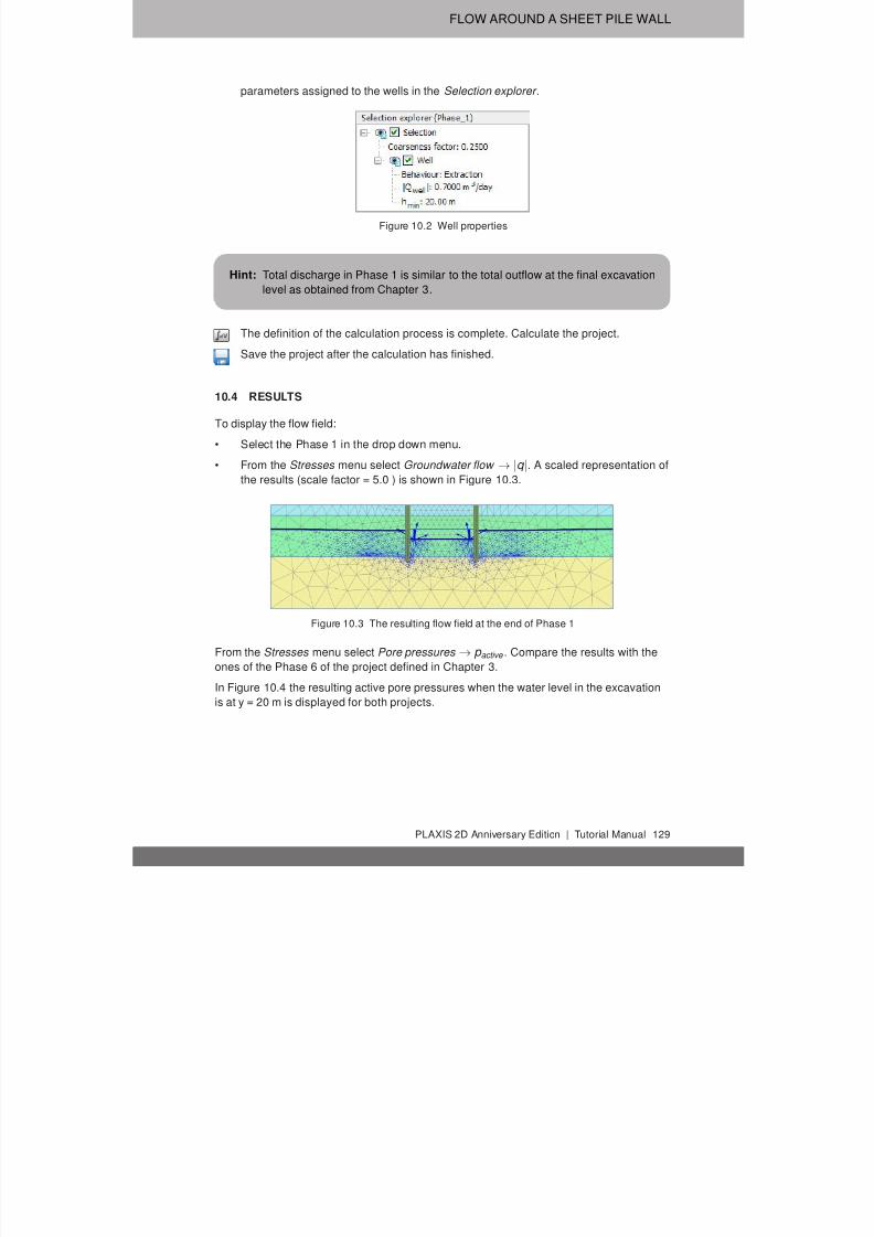
7/21/2019 2DAnniversaryEdition 1 Tutorial
http://slidepdf.com/reader/full/2danniversaryedition-1-tutorial 129/176
FLOW AROUND A SHEET PILE WALL
parameters assigned to the wells in the Selection explorer .
Figure 10.2 Well properties
Hint: Total discharge in Phase 1 is similar to the total outflow at the final excavation
level as obtained from Chapter 3.
The definition of the calculation process is complete. Calculate the project.
Save the project after the calculation has finished.
10.4 RESULTS
To display the flow field:
• Select the Phase 1 in the drop down menu.
• From the Stresses menu select Groundwater flow → |q |. A scaled representation of
the results (scale factor = 5.0 ) is shown in Figure 10.3.
Figure 10.3 The resulting flow field at the end of Phase 1
From the Stresses menu select Pore pressures → p active . Compare the results with the
ones of the Phase 6 of the project defined in Chapter 3.
In Figure 10.4 the resulting active pore pressures when the water level in the excavation
is at y = 20 m is displayed for both projects.
PLAXIS 2D Anniversary Edition | Tutorial Manual 129

7/21/2019 2DAnniversaryEdition 1 Tutorial
http://slidepdf.com/reader/full/2danniversaryedition-1-tutorial 130/176
TUTORIAL MANUAL
a. Active pore pressures (Phase 6 in Chapter 3)
b. Active pore pressures (Phase 1 in the current project)
Figure 10.4 Comparison of the resulting active pore pressures.
130 Tutorial Manual | PLAXIS 2D Anniversary Edition

7/21/2019 2DAnniversaryEdition 1 Tutorial
http://slidepdf.com/reader/full/2danniversaryedition-1-tutorial 131/176
POTATO FIELD MOISTURE CONTENT
11 POTATO FIELD MOISTURE CONTENT
This tutorial demonstrates the applicability of PLAXIS to agricultural problems. The
potato field tutorial involves a loam layer on top of a sandy base. The water level in the
ditches remains unchanged. The precipitation and evaporation may vary on a daily basisdue to weather conditions. The calculation aims to predict the variation of the water
content in the loam layer in time as a result of time-dependent boundary conditions.
precipitation precipitation
sand
loam
15 m15 m0.75 m
0.75 m
0.75 m
0.50 m
1.25 m
Figure 11.1 Potato field geometry
Objectives:
• Defining precipitation
11.1 INPUT
Due to the symmetry of the problem, it is sufficient to simulate a strip with a width of
15.0 m, as indicated in Figure 11.1. The thickness of the loam layer is 2.0 m and the sand
layer is 3.0 m deep.
To create the geometry model, follow these steps:
General settings
• Start the Input program and select Start a new project from the Quick select dialog
box.
• In the Project tabsheet of the Project properties window, enter an appropriate title.• In the Model tabsheet keep the default options for Model (Plane strain ), and
Elements (15-Node ).
• Keep the default values for units and the general parameters.
• Set the model dimensions to x min = 0.0 m, x max = 15.0 m, y min = 0.0 m, y max = 5.0 m
and press OK to close the Project properties window.
PLAXIS 2D Anniversary Edition | Tutorial Manual 131

7/21/2019 2DAnniversaryEdition 1 Tutorial
http://slidepdf.com/reader/full/2danniversaryedition-1-tutorial 132/176
TUTORIAL MANUAL
Definition of soil stratigraphy
Due to the geometry of the model, the options for snapping should be changed.
Click the Snapping options button in the side toolbar.
• In the appearing window set the Number of snap intervals to 100 (Figure 11.2).
• Click OK to close the Snapping window.
Figure 11.2 Modification of the Number of snap intervals
To define the soil stratigraphy:
Create two boreholes located at x = 0.75 and x = 2.00 respectively.
• In the Modify soil layers window add two soil layers.
• In the first borehole set Top = 3.75 and Bottom = 3.00 for the uppermost soil layer.
Set Bottom = 0 for the lowest soil layer.
• In the second borehole set Top = 5.00 and Bottom = 3.0 for the uppermost soil layer.
Set Bottom = 0 for the lowest soil layer.
• For both boreholes the Head is located at y = 4.25. Figure 11.3 shows the soil
stratigraphy defined in the Modify water levels window.
Figure 11.3 Soil stratigraphy in the Modify soil layers window
132 Tutorial Manual | PLAXIS 2D Anniversary Edition

7/21/2019 2DAnniversaryEdition 1 Tutorial
http://slidepdf.com/reader/full/2danniversaryedition-1-tutorial 133/176
POTATO FIELD MOISTURE CONTENT
Create the material data sets according to Table 11.1.
• Assign the material data set to the corresponding clusters in the model.
Table 11.1 Material properties for potato field
Parameter Name Loam Sand UnitGeneral
Material model - Linear elastic Linear elastic -
Type of material behaviour Type Drained Drained -
Soil unit weight above p.l. γ unsat 19 20 kN/m3
Soil unit weight below p.l. γ sat 19 20 kN/m3
Parameters
Young's modulus E ' 1.0·103 1.0·104 kN/m2
Poisson's ratio ν ' 0.3 0.3 -
Flow parameters
Data set Type Staring Staring -
Model - Van Genuchten Van Genuchten -
Subsoil/Topsoil - Topsoil Subsoil -
Type - Clayey loam Loamy sand -
Set parameters to default - Yes Yes -
Horizontal permeability k x 0.01538 0.1270 m/day
Vertical permeability k y 0.01538 0.1270 m/day
11.2 MESH GENERATION
• Proceed to the Mesh mode.
• Multi-select the line segments composing the upper boundary of the model (Figure
11.4).
Figure 11.4 The upper boundary of the model
• In the Selection explorer set the Coarseness factor parameter to 0.5.
Create the mesh. Use the default option for the Element distribution parameter
(Medium ).
View the mesh. The resulting mesh is displayed in (Figure 11.5).
• Click on the Close tab to close the Output program.
PLAXIS 2D Anniversary Edition | Tutorial Manual 133

7/21/2019 2DAnniversaryEdition 1 Tutorial
http://slidepdf.com/reader/full/2danniversaryedition-1-tutorial 134/176
TUTORIAL MANUAL
Figure 11.5 Potato field mesh
11.3 CALCULATIONS
The calculation process consists of two phases. In the initial phase, the groundwater flow
in steady state is calculated. In Phase 1, the transient groundwater flow is calculated.
Initial phase
• Proceed to the Staged construction mode. In this project only groundwater flow
analysis will be performed.
• In the Phases window select the Groundwater flow only option as the Calculation
type in the General subtree.
• The default values of the remaining parameters are valid for this phase. Click OK to
close the Phases window.
Right-click the bottom boundary of the model and select the Activate option in the
appearing menu.
• In the Selection explorer select the Head option in the Behaviour drop-down menu
and set h ref to 3.0 (Figure 11.6).
Figure 11.6 Boundary conditions at the bottom of the geometry model
• In the Model explorer expand the Model conditions subtree.
• Expand the GroundwaterFlow subtree. Set BoundaryXMin and BoundaryXMax to
Closed .
• Expand the Water subtree. The borehole water level is assigned to
GlobalWaterLevel .
Transient phase
In the transient phase the time-dependent variation of precipitation is defined.
134 Tutorial Manual | PLAXIS 2D Anniversary Edition

7/21/2019 2DAnniversaryEdition 1 Tutorial
http://slidepdf.com/reader/full/2danniversaryedition-1-tutorial 135/176
POTATO FIELD MOISTURE CONTENT
Hint: Note that the conditions explicitly assigned to groundwater flow boundaries
are taken into account. In this tutorial the specified Head will be considered
for the bottom boundary of the model, NOT the Closed condition specified in
the GroundwaterFlow subtree under the Model conditions .
Add a new calculation phase.
• In General subtree of the Phases window select the Transient groundwater flow as
Pore pressure calculation type .
• Set the Time interval to 15 days.
• In the Numerical control parameters subtree set the Max number of steps stored to
250. The default values of the remaining parameters will be used.
• Click OK to close the Phases window.To define the precipitation data a discharge function should be defined.
• In the Model explorer expand the Attributes library subtree.
• Right-click on Flow functions and select the Edit option in the appearing menu. The
Flow functions window pops up.
• In the Discharge functions tabsheet add a new function.
• Specify a name for the function and select the Table option in the Signal drop-down
menu.
• Click the Add row button to introduce a new row in the table. Complete the datausing the values given in the Table 11.2.
Table 11.2 Precipitation data
ID Time [day] ∆Discharge [m3 /day]
1 0 0
2 1 1·10-2
3 2 3·10-2
4 3 0
5 4 -2·10-2
6 5 0
7 6 1·10-2
8 7 1·10-2
9 8 0
10 9 -2·10-2
11 10 -2·10-2
12 11 -2·10-2
13 12 -1·10-2
14 13 -1·10-2
15 14 0
16 15 0
• Figure 11.7 shows the defined function for precipitation. Close the windows by
clicking OK .• In the Model explorer expand the Precipitation subtree under Model conditions and
activate it. The default values for discharge (q ) and condition parameters (ψmin =
PLAXIS 2D Anniversary Edition | Tutorial Manual 135
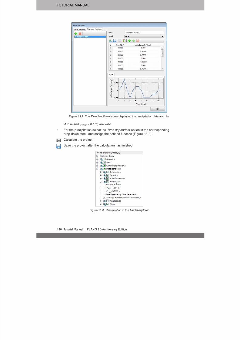
7/21/2019 2DAnniversaryEdition 1 Tutorial
http://slidepdf.com/reader/full/2danniversaryedition-1-tutorial 136/176
TUTORIAL MANUAL
Figure 11.7 The Flow function window displaying the precipitation data and plot
-1.0 m and ψmax = 0.1m) are valid.• For the precipitation select the Time dependent option in the corresponding
drop-down menu and assign the defined function (Figure 11.8).
Calculate the project.
Save the project after the calculation has finished.
Figure 11.8 Precipitation in the Model explorer
136 Tutorial Manual | PLAXIS 2D Anniversary Edition

7/21/2019 2DAnniversaryEdition 1 Tutorial
http://slidepdf.com/reader/full/2danniversaryedition-1-tutorial 137/176
POTATO FIELD MOISTURE CONTENT
Hint: Negative values of precipitation indicate evaporation.
11.4 RESULTS
The calculation was focused on the time-dependent saturation of the potato field. To view
the results:
• From the Stresses menu select Groundwater flow → Saturation .
• Double click the legend. The Legend settings window pops up. Define the settings
as shown in Figure 11.9.
Figure 11.9 Value for settings
• Figure 11.10 shows the spatial distribution of the saturation for the last time step.
Figure 11.10 Saturation field at day 15
• Create an animation of the the transient phase for a better visualisation of the
results.
• It is also interesting to create a vertical cross section at x = 4 m and draw cross
section curves for pore pressure and saturation.
PLAXIS 2D Anniversary Edition | Tutorial Manual 137

7/21/2019 2DAnniversaryEdition 1 Tutorial
http://slidepdf.com/reader/full/2danniversaryedition-1-tutorial 138/176
TUTORIAL MANUAL
138 Tutorial Manual | PLAXIS 2D Anniversary Edition

7/21/2019 2DAnniversaryEdition 1 Tutorial
http://slidepdf.com/reader/full/2danniversaryedition-1-tutorial 139/176
DYNAMIC ANALYSIS OF A GENERATOR ON AN ELASTIC FOUNDATION
12 DYNAMIC ANALYSIS OF A GENERATOR ON AN ELASTIC FOUNDATION
Using PLAXIS, it is possible to simulate dynamic soil-structure interaction. Here the
influence of a vibrating source on its surrounding soil is studied. The vibrating source is a
generator founded on a 0.2 m thick concrete footing of 1 m in diameter, see Figure 12.1.Oscillations caused by the generator are transmitted through the footing into the subsoil.
sandy clay
1m
generator
Figure 12.1 Generator founded on elastic subsoil
The physical damping due to the viscous effects is taken into consideration via the
Rayleigh damping. Also, due to axisymmetry 'geometric damping' can be significant in
attenuating the vibration.The modelling of the boundaries is one of the key points. In order to avoid spurious wave
reflections at the model boundaries (which do not exist in reality), special conditions have
to be applied in order to absorb waves reaching the boundaries.
Objectives:
• Defining a Dynamic calculation.
• Defining Dynamic loads.
• Defining material damping by means of Rayleigh damping.
12.1 INPUT
To create the geometry model, follow these steps:
General settings
• Start the Input program and select Start a new project from the Quick select dialog
box.
• In the Project tabsheet of the Project properties window, enter an appropriate title.
• Due to the three dimensional nature of the problem, an axisymmetric model is used.In the Model tabsheet select the Axisymmetric option for Model and keep the
default option for Elements (15-Noded ).
PLAXIS 2D Anniversary Edition | Tutorial Manual 139
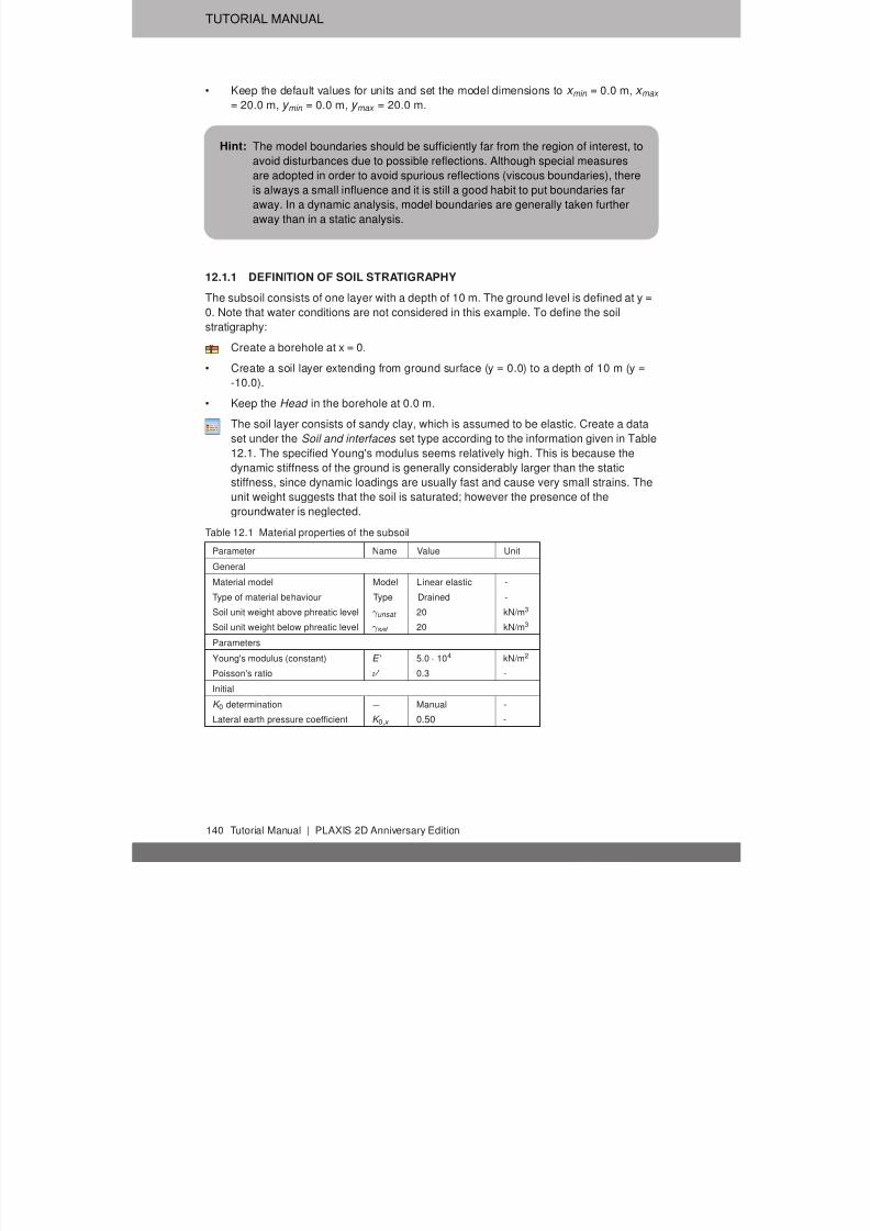
7/21/2019 2DAnniversaryEdition 1 Tutorial
http://slidepdf.com/reader/full/2danniversaryedition-1-tutorial 140/176
TUTORIAL MANUAL
• Keep the default values for units and set the model dimensions to x min = 0.0 m, x max
= 20.0 m, y min = 0.0 m, y max = 20.0 m.
Hint: The model boundaries should be sufficiently far from the region of interest, toavoid disturbances due to possible reflections. Although special measures
are adopted in order to avoid spurious reflections (viscous boundaries), there
is always a small influence and it is still a good habit to put boundaries far
away. In a dynamic analysis, model boundaries are generally taken further
away than in a static analysis.
12.1.1 DEFINITION OF SOIL STRATIGRAPHY
The subsoil consists of one layer with a depth of 10 m. The ground level is defined at y =0. Note that water conditions are not considered in this example. To define the soil
stratigraphy:
Create a borehole at x = 0.
• Create a soil layer extending from ground surface (y = 0.0) to a depth of 10 m (y =
-10.0).
• Keep the Head in the borehole at 0.0 m.
The soil layer consists of sandy clay, which is assumed to be elastic. Create a data
set under the Soil and interfaces set type according to the information given in Table
12.1. The specified Young's modulus seems relatively high. This is because thedynamic stiffness of the ground is generally considerably larger than the static
stiffness, since dynamic loadings are usually fast and cause very small strains. The
unit weight suggests that the soil is saturated; however the presence of the
groundwater is neglected.
Table 12.1 Material properties of the subsoil
Parameter Name Value Unit
General
Material model Model Linear elastic -
Type of material behaviour Type Drained -
Soil unit weight above phreatic level γ unsat 20 kN/m3
Soil unit weight below phreatic level γ sat 20 kN/m3
Parameters
Young's modulus (constant) E ' 5.0 · 104 kN/m2
Poisson's ratio ν ' 0.3 -
Initial
K 0 determination − Manual -
Lateral earth pressure coefficient K 0,x 0.50 -
140 Tutorial Manual | PLAXIS 2D Anniversary Edition

7/21/2019 2DAnniversaryEdition 1 Tutorial
http://slidepdf.com/reader/full/2danniversaryedition-1-tutorial 141/176
DYNAMIC ANALYSIS OF A GENERATOR ON AN ELASTIC FOUNDATION
Hint: When using Mohr-Coulomb or linear elastic models the wave velocities V p
and V s are calculated from the elastic parameters and the soil weight. V p
and V s can also be entered as input; the elastic parameters are then
calculated automatically. See also Elastic parameters and the Wave Velocityrelationships in Section ?? of the Reference Manual.
12.1.2 DEFINITION OF STRUCTURAL ELEMENTS
The generator is defined in the Structures mode.
Create a plate extending from (0.0 0.0) to (0.5 0.0) to represent the footing.
Define a material data set for the footing according to the information given in Table
12.2. The footing is assumed to be elastic and has a weight of 5 kN/m 2.
Table 12.2 Material properties of the footing
Parameter Name Value Unit
Material type Type Elastic; Isotropic -
Normal stiffness EA 7.6 · 106 kN/m
Flexural rigidity EI 2.4 · 104 kNm2 /m
Weight w 5.0 kN/m/m
Poisson's ratio ν 0.0 -
• Apply a distributed load on the footing to model the weight of the generator as well
as the vibrations that it produces. The actual value of the load will be defined later.
The model is shown in Figure 12.2.
Figure 12.2 Model layout
12.2 MESH GENERATION
• Proceed to the Mesh mode.Generate the mesh. Use the default option for the Element distribution parameter
(Medium ).
PLAXIS 2D Anniversary Edition | Tutorial Manual 141

7/21/2019 2DAnniversaryEdition 1 Tutorial
http://slidepdf.com/reader/full/2danniversaryedition-1-tutorial 142/176
TUTORIAL MANUAL
View the generated mesh. The resulting mesh is shown in Figure 12.3. Note that the
mesh is automatically refined under the footing.
• Click on the Close tab to close the Output program.
Figure 12.3 The generated mesh
12.3 CALCULATIONS
The calculation consists of 4 phases and it will be defined in the Staged construction
mode.
Initial phase • Click the Staged construction tab to proceed with the definition of the calculation
phases.
• The initial phase has already been introduced. The default settings of the initial
phase will be used in this tutorial.
Phase 1
Add a new calculation phase. The default settings of the added phase will be used
for this calculation phase.
• Activate the footing.
• Activate the static component of the distributed load. In the Selection explorer set
q y ,start ,ref value to -8 kN/m/m. Do not activate the dynamic component of the load
(Figure 12.4).
Phase 2
In this phase, a vertical harmonic load, with a frequency of 10 Hz and amplitude of 10
kN/m2, is applied to simulate the vibrations transmitted by the generator. Five cycles with
a total time interval of 0.5 sec are considered.
Add a new calculation phase.
In the General subtree in the Phases window, select the Dynamic option as
calculation type.
142 Tutorial Manual | PLAXIS 2D Anniversary Edition
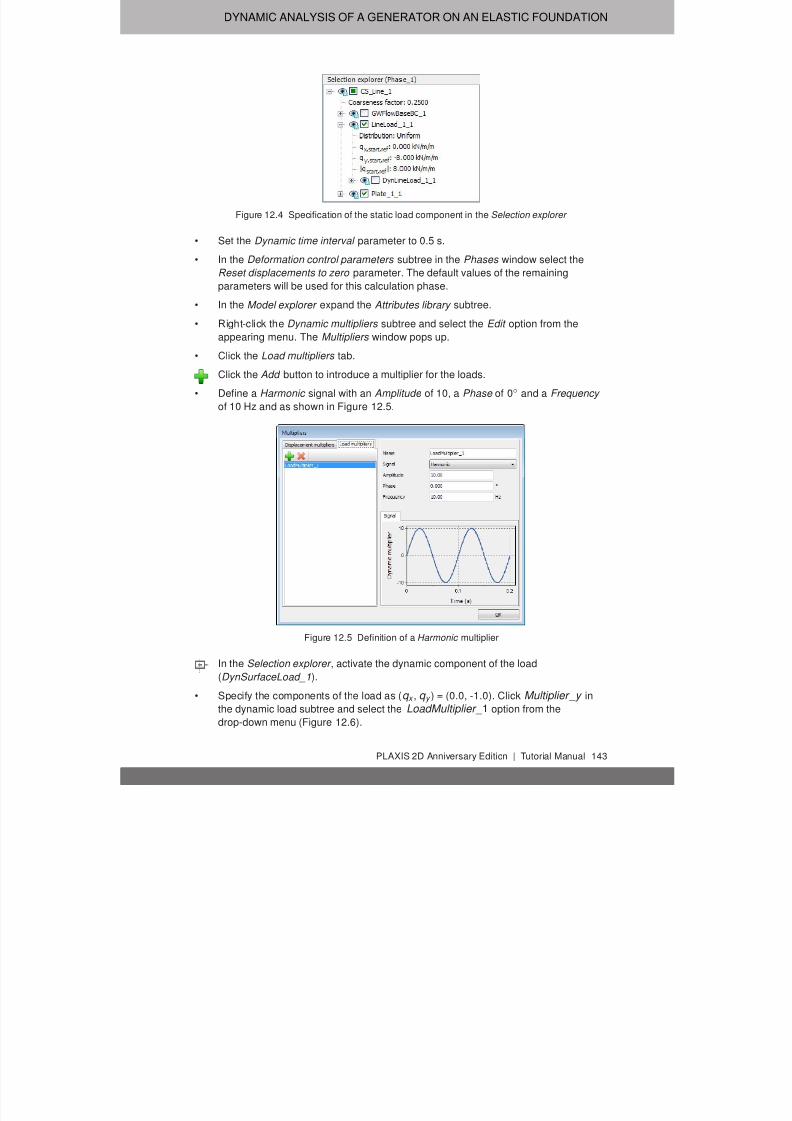
7/21/2019 2DAnniversaryEdition 1 Tutorial
http://slidepdf.com/reader/full/2danniversaryedition-1-tutorial 143/176
DYNAMIC ANALYSIS OF A GENERATOR ON AN ELASTIC FOUNDATION
Figure 12.4 Specification of the static load component in the Selection explorer
• Set the Dynamic time interval parameter to 0.5 s.
• In the Deformation control parameters subtree in the Phases window select the
Reset displacements to zero parameter. The default values of the remainingparameters will be used for this calculation phase.
• In the Model explorer expand the Attributes library subtree.
• Right-click the Dynamic multipliers subtree and select the Edit option from the
appearing menu. The Multipliers window pops up.
• Click the Load multipliers tab.
Click the Add button to introduce a multiplier for the loads.
• Define a Harmonic signal with an Amplitude of 10, a Phase of 0◦ and a Frequency
of 10 Hz and as shown in Figure 12.5.
Figure 12.5 Definition of a Harmonic multiplier
In the Selection explorer , activate the dynamic component of the load
(DynSurfaceLoad_1).
• Specify the components of the load as (q x , q y ) = (0.0, -1.0). Click Multiplier _y in
the dynamic load subtree and select the LoadMultiplier _1 option from the
drop-down menu (Figure 12.6).
PLAXIS 2D Anniversary Edition | Tutorial Manual 143
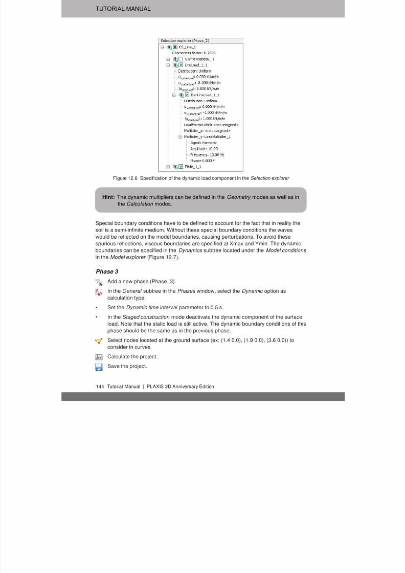
7/21/2019 2DAnniversaryEdition 1 Tutorial
http://slidepdf.com/reader/full/2danniversaryedition-1-tutorial 144/176
TUTORIAL MANUAL
Figure 12.6 Specification of the dynamic load component in the Selection explorer
Hint: The dynamic multipliers can be defined in the Geometry modes as well as in
the Calculation modes.
Special boundary conditions have to be defined to account for the fact that in reality the
soil is a semi-infinite medium. Without these special boundary conditions the waves
would be reflected on the model boundaries, causing perturbations. To avoid these
spurious reflections, viscous boundaries are specified at Xmax and Ymin. The dynamic
boundaries can be specified in the Dynamics subtree located under the Model conditions
in the Model explorer (Figure 12.7).
Phase 3
Add a new phase (Phase_3).In the General subtree in the Phases window, select the Dynamic option as
calculation type.
• Set the Dynamic time interval parameter to 0.5 s.
• In the Staged construction mode deactivate the dynamic component of the surface
load. Note that the static load is still active. The dynamic boundary conditions of this
phase should be the same as in the previous phase.
Select nodes located at the ground surface (ex: (1.4 0.0), (1.9 0.0), (3.6 0.0)) to
consider in curves.
Calculate the project.
Save the project.
144 Tutorial Manual | PLAXIS 2D Anniversary Edition

7/21/2019 2DAnniversaryEdition 1 Tutorial
http://slidepdf.com/reader/full/2danniversaryedition-1-tutorial 145/176
DYNAMIC ANALYSIS OF A GENERATOR ON AN ELASTIC FOUNDATION
Figure 12.7 Boundary conditions for Dynamic calculations
12.3.1 ADDITIONAL CALCULATION WITH DAMPING
In a second calculation, material damping is introduced by means of Rayleigh damping.
Rayleigh damping can be entered in the material data set. The following steps are
necessary:
• Save the project under another name.
• Open the material data set of the soil.
• In the General tabsheet click the box next to the Rayleigh α parameter. Note that the
display of the General tabsheet has changed displaying the Single DOF equivalence
box.
• In order to introduce 5% of material damping, set the value of the ξ parameter to 5%
for both targets and set the frequency values to 1 and 10 for the Target 1 and Target
2 respectively.
• Click on one of the definition cells of the Rayleigh parameters. The values of α and
β are automatically calculated by the program.
• Click OK to close the data base.
• Check whether the phases are properly defined (according to the information given
before) and start the calculation.
PLAXIS 2D Anniversary Edition | Tutorial Manual 145

7/21/2019 2DAnniversaryEdition 1 Tutorial
http://slidepdf.com/reader/full/2danniversaryedition-1-tutorial 146/176
TUTORIAL MANUAL
Figure 12.8 Input of Rayleigh damping
12.4 RESULTS
The Curve generator feature is particularly useful for dynamic analysis. You can easily
display the actual loading versus time (input) and also displacements, velocities and
accelerations of the pre-selected points versus time. The evolution of the defined
multipliers with time can be plotted by assigning Dynamic time to the x-axis and u y to the
y-axis. Figure 12.9 shows the response of the pre-selected points at the surface of the
structure. It can be seen that even with no damping, the waves are dissipated which can
be attributed to the geometric damping.
The presence of damping is clear in Figure 12.10. It can be seen that the vibration is
totally seized when some time is elapsed after the removal of the force (at t = 0.5 s).
Also, the displacement amplitudes are lower. Compare Figure 12.10 (without damping)
with Figure 12.10 (with damping).
It is possible in the Output program to display displacements, velocities and accelerations
at a particular time, by choosing the appropriate option in the Deformations menu. Figure
12.11 shows the total accelerations in the soil at the end of phase 2 (t = 0.5 s).
146 Tutorial Manual | PLAXIS 2D Anniversary Edition

7/21/2019 2DAnniversaryEdition 1 Tutorial
http://slidepdf.com/reader/full/2danniversaryedition-1-tutorial 147/176
DYNAMIC ANALYSIS OF A GENERATOR ON AN ELASTIC FOUNDATION
Figure 12.9 Vertical displ.- time on the surface at different distances to the vibrating source (without
damping)
Figure 12.10 Vertical displ.- time on the surface at different distances to the vibrating source (with
damping)
PLAXIS 2D Anniversary Edition | Tutorial Manual 147
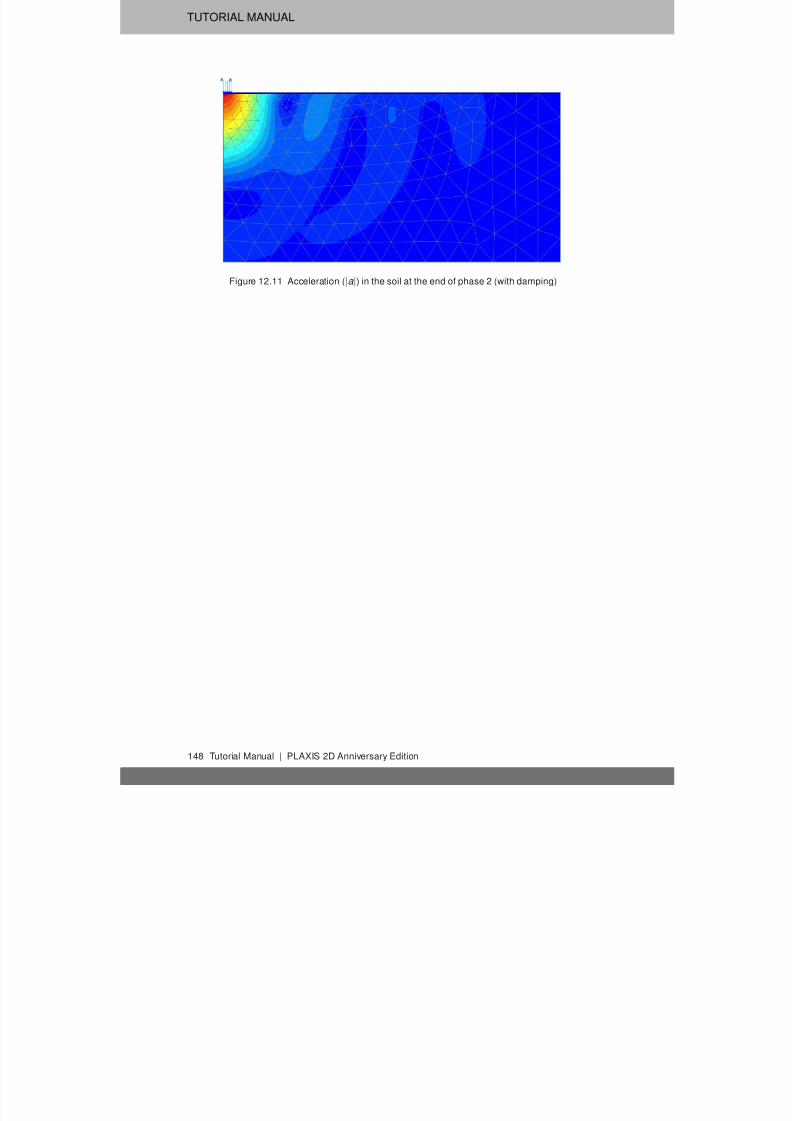
7/21/2019 2DAnniversaryEdition 1 Tutorial
http://slidepdf.com/reader/full/2danniversaryedition-1-tutorial 148/176
TUTORIAL MANUAL
Figure 12.11 Acceleration (|a |) in the soil at the end of phase 2 (with damping)
148 Tutorial Manual | PLAXIS 2D Anniversary Edition
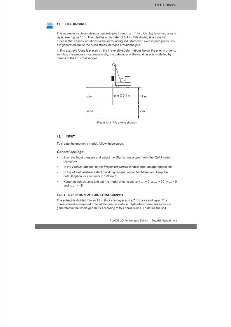
7/21/2019 2DAnniversaryEdition 1 Tutorial
http://slidepdf.com/reader/full/2danniversaryedition-1-tutorial 149/176
PILE DRIVING
13 PILE DRIVING
This example involves driving a concrete pile through an 11 m thick clay layer into a sand
layer, see Figure 13.1. The pile has a diameter of 0.4 m. Pile driving is a dynamic
process that causes vibrations in the surrounding soil. Moreover, excess pore pressuresare generated due to the quick stress increase around the pile.
In this example focus is placed on the irreversible deformations below the pile. In order to
simulate this process most realistically, the behaviour of the sand layer is modelled by
means of the HS small model.
clay
sand
pile Ø 0.4 m 11 m
7 m
Figure 13.1 Pile driving situation
13.1 INPUT
To create the geometry model, follow these steps:
General settings
• Start the Input program and select the Start a new project from the Quick select
dialog box.
• In the Project tabsheet of the Project properties window enter an appropriate title.
• In the Model tabsheet select the Axisymmetric option for Model and keep the
default option for Elements (15-Noded ).
• Keep the default units and set the model dimensions to x min = 0, x max = 30, y min = 0
and y max = 18.
13.1.1 DEFINITION OF SOIL STRATIGRAPHY
The subsoil is divided into an 11 m thick clay layer and a 7 m thick sand layer. Thephreatic level is assumed to be at the ground surface. Hydrostatic pore pressures are
generated in the whole geometry according to this phreatic line. To define the soil
PLAXIS 2D Anniversary Edition | Tutorial Manual 149
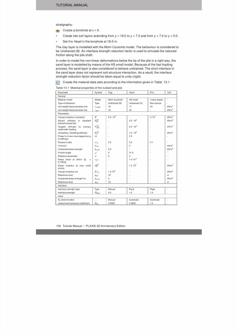
7/21/2019 2DAnniversaryEdition 1 Tutorial
http://slidepdf.com/reader/full/2danniversaryedition-1-tutorial 150/176
TUTORIAL MANUAL
stratigraphy:
Create a borehole at x = 0.
• Create two soil layers extending from y = 18.0 to y = 7.0 and from y = 7.0 to y = 0.0.
• Set the Head in the borehole at 18.0 m.
The clay layer is modelled with the Mohr-Coulomb model. The behaviour is considered to
be Undrained (B). An interface strength reduction factor is used to simulate the reduced
friction along the pile shaft.
In order to model the non-linear deformations below the tip of the pile in a right way, the
sand layer is modelled by means of the HS small model. Because of the fast loading
process, the sand layer is also considered to behave undrained. The short interface in
the sand layer does not represent soil-structure interaction. As a result, the interface
strength reduction factor should be taken equal to unity (rigid).
Create the material data sets according to the information given in Table 13.1.
Table 13.1 Material properties of the subsoil and pile
Parameter Symbol Clay Sand Pile Unit
General
Material model Model Mohr-Coulomb HS small Linear elastic -
Type of behaviour Type Undrained (B) Undrained (A) Non-porous -
Unit weight above phreatic line γ unsat 16 17 24 kN/m3
Unit weight below phreatic line γ sat 18 20 - kN/m3
Parameters
Young's modulus (constant) E ' 5.0· 103 - 3·107 kN/m2
Secant stiffness in standard
drained triaxial test
E ref 50 - 5.0· 104 - kN/m2
Tangent stiffness for primaryoedometer loading
E ref oed - 5.0· 104 - kN/m2
Unloading / reloading stiffness E ref ur - 1.5· 105 - kN/m2
Power for stress-level dependencyof stiffness
m - 0.5 - -
Poisson's ratio ν 'ur 0.3 0.2 0.1 -
Cohesion c 'ref - 0 - kN/m2
Undrained shear strength s u ,ref 5.0 - - kN/m2
Friction angle ϕ' 0 31.0 - ◦
Dilatancy parameter ψ 0 0 - ◦
Shear strain at which G s =0.722G 0
γ 0.7 - 1.0·10-4 - -
Shear modulus at very smallstrains
G ref 0 - 1.2·105 - kN/m2
Young's modulus inc. E 'inc 1.0·103 - - kN/m2
Reference level y ref 18 - - m
Undrained shear strength inc. s u ,inc 3 - - kN/m2
Reference level y ref 18 - - m
Interface
Interface strength type Type Manual Rigid Rigid -
Interface strength R inter 0.5 1.0 1.0 -
Initial
K 0 determination − Manual Automatic Automatic -
Lateral earth pressure coefficient K 0,x 0.5000 0.4850 1.0 -
150 Tutorial Manual | PLAXIS 2D Anniversary Edition
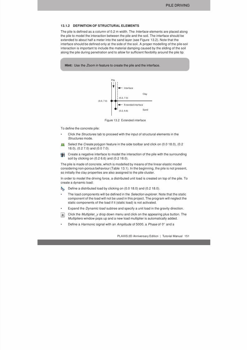
7/21/2019 2DAnniversaryEdition 1 Tutorial
http://slidepdf.com/reader/full/2danniversaryedition-1-tutorial 151/176
PILE DRIVING
13.1.2 DEFINITION OF STRUCTURAL ELEMENTS
The pile is defined as a column of 0.2 m width. The Interface elements are placed along
the pile to model the interaction between the pile and the soil. The interface should be
extended to about half a meter into the sand layer (see Figure 13.2). Note that the
interface should be defined only at the side of the soil. A proper modelling of the pile-soilinteraction is important to include the material damping caused by the sliding of the soil
along the pile during penetration and to allow for sufficient flexibility around the pile tip.
Hint: Use the Zoom in feature to create the pile and the interface.
Pile
Interface
Clay
Extended interface
Sand
(0.0, 7.0)
(0.2, 7.0)
(0.2, 6.6)
Figure 13.2 Extended interface
To define the concrete pile:• Click the Structures tab to proceed with the input of structural elements in the
Structures mode.
Select the Create polygon feature in the side toolbar and click on (0.0 18.0), (0.2
18.0), (0.2 7.0) and (0.0 7.0).
Create a negative interface to model the interaction of the pile with the surrounding
soil by clicking on (0.2 6.6) and (0.2 18.0).
The pile is made of concrete, which is modelled by means of the linear elastic model
considering non-porous behaviour (Table 13.1). In the beginning, the pile is not present,
so initially the clay properties are also assigned to the pile cluster.
In order to model the driving force, a distributed unit load is created on top of the pile. To
create a dynamic load:
Define a distributed load by clicking on (0.0 18.0) and (0.2 18.0).
• The load components will be defined in the Selection explorer . Note that the static
component of the load will not be used in this project. The program will neglect the
static components of the load if it (static load) is not activated.
• Expand the Dynamic load subtree and specify a unit load in the gravity direction.
Click the Multiplier_y drop down menu and click on the appearing plus button. TheMultipliers window pops up and a new load multiplier is automatically added.
• Define a Harmonic signal with an Amplitude of 5000, a Phase of 0◦ and a
PLAXIS 2D Anniversary Edition | Tutorial Manual 151

7/21/2019 2DAnniversaryEdition 1 Tutorial
http://slidepdf.com/reader/full/2danniversaryedition-1-tutorial 152/176
TUTORIAL MANUAL
Frequency of 50 Hz and as shown in Figure 12.5.
Figure 13.3 Definition of a Harmonic multiplier
Hint: Note that dynamic multipliers can be defined by right-clicking the Dynamic
multipliers subtree under Attributes library in the Model explorer .
» Note that dynamic multipliers are attributes and as such it is possible to
define them in all the program modes.
The final geometry model is shown in Figure 13.4.
Figure 13.4 The geometry model
152 Tutorial Manual | PLAXIS 2D Anniversary Edition
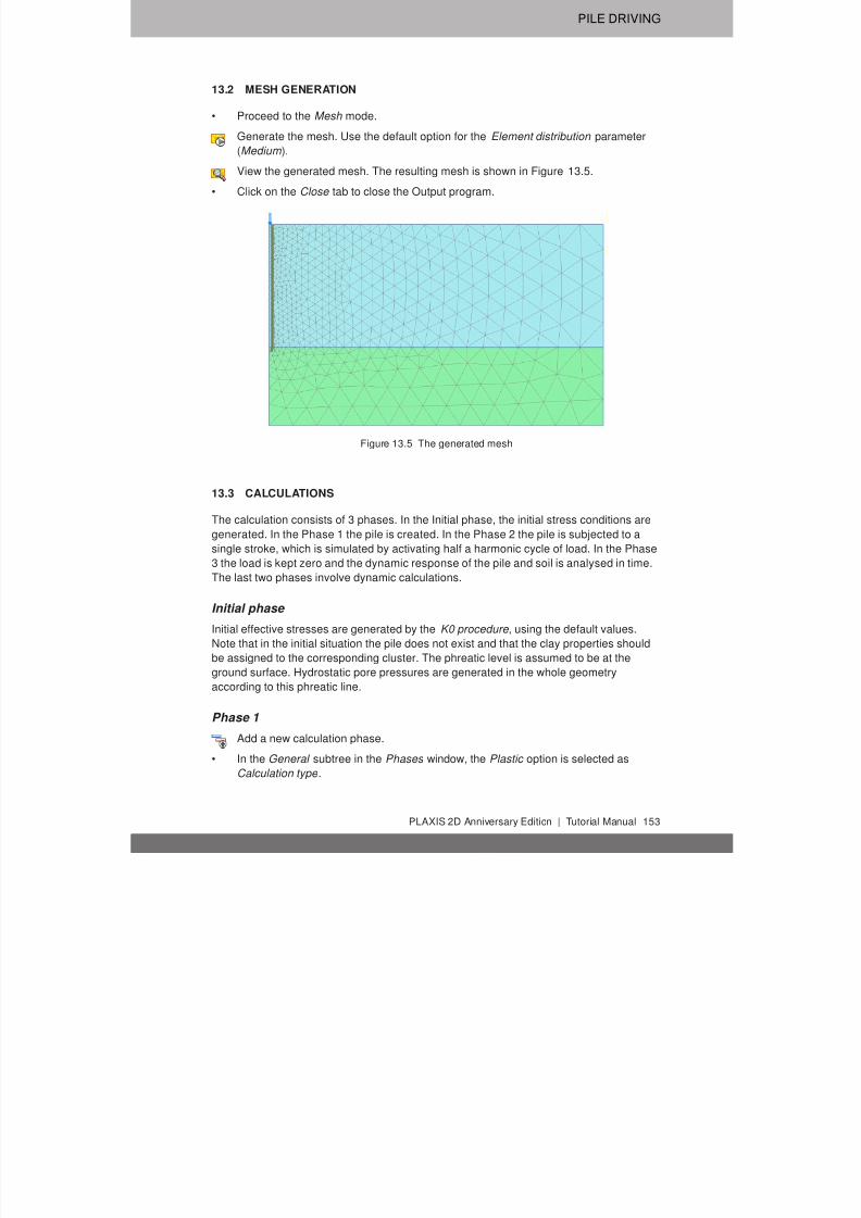
7/21/2019 2DAnniversaryEdition 1 Tutorial
http://slidepdf.com/reader/full/2danniversaryedition-1-tutorial 153/176
PILE DRIVING
13.2 MESH GENERATION
• Proceed to the Mesh mode.
Generate the mesh. Use the default option for the Element distribution parameter
(Medium ).
View the generated mesh. The resulting mesh is shown in Figure 13.5.
• Click on the Close tab to close the Output program.
Figure 13.5 The generated mesh
13.3 CALCULATIONS
The calculation consists of 3 phases. In the Initial phase, the initial stress conditions are
generated. In the Phase 1 the pile is created. In the Phase 2 the pile is subjected to a
single stroke, which is simulated by activating half a harmonic cycle of load. In the Phase
3 the load is kept zero and the dynamic response of the pile and soil is analysed in time.
The last two phases involve dynamic calculations.
Initial phase
Initial effective stresses are generated by the K0 procedure , using the default values.
Note that in the initial situation the pile does not exist and that the clay properties should
be assigned to the corresponding cluster. The phreatic level is assumed to be at the
ground surface. Hydrostatic pore pressures are generated in the whole geometry
according to this phreatic line.
Phase 1
Add a new calculation phase.
• In the General subtree in the Phases window, the Plastic option is selected as
Calculation type .
PLAXIS 2D Anniversary Edition | Tutorial Manual 153

7/21/2019 2DAnniversaryEdition 1 Tutorial
http://slidepdf.com/reader/full/2danniversaryedition-1-tutorial 154/176
TUTORIAL MANUAL
• The Staged construction option is by default selected as Loading type .
• In the Staged construction mode assign the pile properties to the pile cluster.
• Activate the interface. The model for the Phase 1 in the Staged construction mode is
displayed in Figure 13.6.
Figure 13.6 Configuration of Phase 1 in the Staged construction mode
Phase 2 Add a new calculation phase.
• In the General subtree in the Phases window, select the Dynamic option as
Calculation type .
• Set the Dynamic time interval to 0.01 s.
• In the Deformation control parameters subtree select Reset displacements to zero .
• In the Staged construction mode activate the dynamic component of the distributed
load. The activated dynamic component of the load in Selection explorer is shown in
Figure 13.7.
• Expand the Dynamics subtree under Model conditions in the Model explorer .
• Specify viscous boundaries at x max and y min (Figure 13.8).
The result of this phase is half a harmonic cycle of the external load. At the end of this
phase, the load is back to zero.
Phase 3
Add a new calculation phase.
• In the General subtree in the Phases window, select the Dynamic option as
Calculation type .
• Set the Dynamic time interval to 0.19 s.
154 Tutorial Manual | PLAXIS 2D Anniversary Edition

7/21/2019 2DAnniversaryEdition 1 Tutorial
http://slidepdf.com/reader/full/2danniversaryedition-1-tutorial 155/176
PILE DRIVING
Figure 13.7 The dynamic load component in the Selection explorer
Figure 13.8 Boundary conditions for Dynamic calculations
• In the Staged construction mode de-activate the dynamic load.
Select a node at the top of the pile for load displacement curves.
Calculate the project.
Save the project.
PLAXIS 2D Anniversary Edition | Tutorial Manual 155
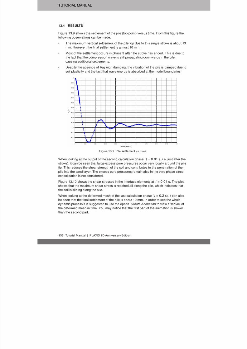
7/21/2019 2DAnniversaryEdition 1 Tutorial
http://slidepdf.com/reader/full/2danniversaryedition-1-tutorial 156/176
TUTORIAL MANUAL
13.4 RESULTS
Figure 13.9 shows the settlement of the pile (top point) versus time. From this figure the
following observations can be made:
• The maximum vertical settlement of the pile top due to this single stroke is about 13mm. However, the final settlement is almost 10 mm.
• Most of the settlement occurs in phase 3 after the stroke has ended. This is due to
the fact that the compression wave is still propagating downwards in the pile,
causing additional settlements.
• Despite the absence of Rayleigh damping, the vibration of the pile is damped due to
soil plasticity and the fact that wave energy is absorbed at the model boundaries.
Figure 13.9 Pile settlement vs. time
When looking at the output of the second calculation phase (t = 0.01 s, i.e. just after the
stroke), it can be seen that large excess pore pressures occur very locally around the pile
tip. This reduces the shear strength of the soil and contributes to the penetration of the
pile into the sand layer. The excess pore pressures remain also in the third phase sinceconsolidation is not considered.
Figure 13.10 shows the shear stresses in the interface elements at t = 0.01 s. The plot
shows that the maximum shear stress is reached all along the pile, which indicates that
the soil is sliding along the pile.
When looking at the deformed mesh of the last calculation phase (t = 0.2 s), it can also
be seen that the final settlement of the pile is about 10 mm. In order to see the whole
dynamic process it is suggested to use the option Create Animation to view a 'movie' of
the deformed mesh in time. You may notice that the first part of the animation is slower
than the second part.
156 Tutorial Manual | PLAXIS 2D Anniversary Edition

7/21/2019 2DAnniversaryEdition 1 Tutorial
http://slidepdf.com/reader/full/2danniversaryedition-1-tutorial 157/176
PILE DRIVING
Figure 13.10 Maximum shear stresses in the interface at t = 0.01 s.
PLAXIS 2D Anniversary Edition | Tutorial Manual 157

7/21/2019 2DAnniversaryEdition 1 Tutorial
http://slidepdf.com/reader/full/2danniversaryedition-1-tutorial 158/176
TUTORIAL MANUAL
158 Tutorial Manual | PLAXIS 2D Anniversary Edition

7/21/2019 2DAnniversaryEdition 1 Tutorial
http://slidepdf.com/reader/full/2danniversaryedition-1-tutorial 159/176
FREE VIBRATION AND EARTHQUAKE ANALYSIS OF A BUILDING
14 FREE VIBRATION AND EARTHQUAKE ANALYSIS OF A BUILDING
This example demonstrates the natural frequency of a five-storey building when
subjected to free vibration and earthquake loading.
The building consists of 5 floors and a basement. It is 10 m wide and 17 m high including
basement. The total height from the ground level is 5 x 3 m = 15 m and the basement is
2 m deep. A value of 5 kN/m2 is taken as the weight of the floors and the walls. The
building is constructed on a clay layer of 15 m depth underlayed by a deep sand layer. In
the model, 25 m of the sand layer will be considered.
14.1 INPUT
General settings
• Start the Input program and select the Start a new project from the Quick select
dialog box.
• In the Project tabsheet of the Project properties window enter an appropriate title.
• In the Model tabsheet keep the default options for Model (Plane strain ) and
Elements (15-Noded ).
• Keep the default units and set the model dimensions to x min = -80.0, x max = 80.0,
y min = -40.0 and y max = 15.0.
x
y15 m
15 m
25 m
75 m75 m 10 m
2 m
Figure 14.1 Geometry of the project
14.1.1 DEFINITION OF SOIL STRATIGRAPHY
The subsoil is divided into an 15 m thick clayey layer and a 25 m thick sandy layer. The
phreatic level is assumed to be at y = -15.0 m. Hydrostatic pore pressures are generated
in the whole geometry according to this phreatic line.
Create a borehole at x = 0. The Modify soil layers window pops up.
• Add two soil layers extending from y = 0.0 to y = -15.0 and from y = -15.0 to y = -40.
• Set the Head in the borehole at -15.0 m.
The upper layer consists of mostly clayey soil and the lower one is sandy. Both have HS
small model properties. The presence of the groundwater is neglected. The soil layers
PLAXIS 2D Anniversary Edition | Tutorial Manual 159

7/21/2019 2DAnniversaryEdition 1 Tutorial
http://slidepdf.com/reader/full/2danniversaryedition-1-tutorial 160/176
TUTORIAL MANUAL
with HS small model properties have inherent hysteretic damping.
Open the Material sets window.
• Create data sets under Soil and interfaces set type according to the information
given in Table 14.1.• Assign the material datasets to the corresponding soil layers in the borehole.
Table 14.1 Material properties of the subsoil layers
Parameter Name Upper clayeylayer
Lower sandylayer
Unit
General
Material model Model HS small HS small -
Type of material behaviour Type Drained Drained -
Soil unit weight above phreaticlevel
γ unsat 16 20 kN/m3
Soil unit weight above phreaticlevel
γ sat 20 20 kN/m3
Parameters
Secant stiffness in standarddrained triaxial test
E ref 50 2.0·104 3.0·104 kN/m2
Tangent stiffness for primaryoedometer loading
E ref oed 2.561·104 3.601·104 kN/m2
Unloading / reloading stiffness E ref ur 9.484·104 1.108·105 kN/m2
Power for stress-level dependencyof stiffness
m 0.5 0.5 -
Cohesion c 'ref 10 5 kN/m2
Friction angle ϕ' 18 28 ◦
Dilatancy angle ψ 0 0 ◦
Shear strain at which G s =
0.722G 0
γ 0.7 1.2·10-4 1.5·10-4 -
Shear modulus at very small
strains
G ref 0 2.7·105 1.0·105 kN/m2
Poisson's ratio ν 'ur 0.2 0.2 -
When subjected to cyclic shear loading, the HS small model will show typical hysteretic
behaviour. Starting from the small-strain shear stiffness, G ref 0 , the actual stiffness will
decrease with increasing shear. Figures 14.2 and 14.3 display the Modulus reduction
curves, i.e. the decay of the shear modulus with strain. The upper curve shows the
secant shear modulus and the lower curve shows the tangent shear modulus.
In the HS small model, the tangent shear modulus is bounded by a lower limit, G ur .
G ur = E ur
2(1 + ν ur )
The values of G ref ur for the Upper clayey layer and Lower sandy layer and the ratio to G ref
0
are shown in Table 14.2. This ratio determines the maximum damping ratio that can be
obtained.
Table 14.2 G ur values and ratio to G ref 0
Parameter Unit Upper clayeylayer
Lower sandylayer
G ur kN /m 2 39517 41167
G ref 0 /G ur - 6.75 2.5
Figures 14.4 and 14.5 show the damping ratio as a function of the shear strain for the
material used in the model. For a more detailed description and elaboration from the
160 Tutorial Manual | PLAXIS 2D Anniversary Edition
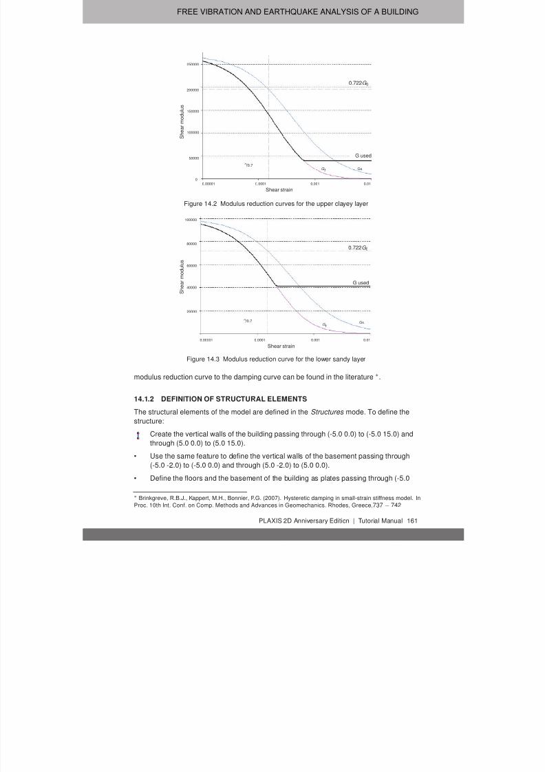
7/21/2019 2DAnniversaryEdition 1 Tutorial
http://slidepdf.com/reader/full/2danniversaryedition-1-tutorial 161/176
FREE VIBRATION AND EARTHQUAKE ANALYSIS OF A BUILDING
0
100000
50000
150000
200000
250000
S h e a r m o d u l u s
Shear strain
0.00001 0.0001 0.001 0.01
G t Gsγ 0.7
0.722G 0
G used
Figure 14.2 Modulus reduction curves for the upper clayey layer
20000
40000
60000
80000
100000
S h e a r m o d u l u s
Shear strain
0.00001 0.0001 0.001 0.01
G t Gs
γ 0.7
0.722G 0
G used
Figure 14.3 Modulus reduction curve for the lower sandy layer
modulus reduction curve to the damping curve can be found in the literature
∗
.
14.1.2 DEFINITION OF STRUCTURAL ELEMENTS
The structural elements of the model are defined in the Structures mode. To define the
structure:
Create the vertical walls of the building passing through (-5.0 0.0) to (-5.0 15.0) and
through (5.0 0.0) to (5.0 15.0).
• Use the same feature to define the vertical walls of the basement passing through
(-5.0 -2.0) to (-5.0 0.0) and through (5.0 -2.0) to (5.0 0.0).
• Define the floors and the basement of the building as plates passing through (-5.0
∗ Brinkgreve, R.B.J., Kappert, M.H., Bonnier, P.G. (2007). Hysteretic damping in small-strain stiffness model. In
Proc. 10th Int. Conf. on Comp. Methods and Advances in Geomechanics. Rhodes, Greece, 737 − 742
PLAXIS 2D Anniversary Edition | Tutorial Manual 161

7/21/2019 2DAnniversaryEdition 1 Tutorial
http://slidepdf.com/reader/full/2danniversaryedition-1-tutorial 162/176
TUTORIAL MANUAL
0
0.2
0.15
0.1
0.05 D a m p i n g
r a t i o
Cyclic shear strain
0.00001 0.0001 0.001 0.01
Figure 14.4 Damping curve for the upper clayey layer
0
0.2
0.15
0.1
0.05 D a m p i n g r a t i o
Cyclic shear strain
0.00001 0.0001 0.001 0.01
Figure 14.5 Damping curve for the lower sandy layer
-2.0) to (5.0 -2.0), (-5.0 0.0) to (5.0 0.0), (-5.0 3.0) to (5.0 3.0), (-5.0 6.0) to (5.0 6.0),
(-5.0 9.0) to (5.0 9.0), (-5.0 12.0) to (5.0 12.0) and (-5.0 15.0) to (5.0 15.0).
The plates, representing the walls and the floors in the building, are considered to be
linear elastic. Note that two different material datasets are used, one for the basement
and the other for the rest of the building. The physical damping in the building is
simulated by means of Rayleigh damping. A description of Rayleigh damping parameters
is given in Section ?? or the Reference Manual.
Define the material datasets for the structural elements in the building according to
Table 14.3.Table 14.3 Material properties of the building (plate properties)
Parameter Name Rest of building Basement Unit
Material type Type Elastic; Isotropic Elastic; Isotropic -
Normal stiffness EA 9.0·106 1.2·107 kN/m
Flexural rigidity EI 6.75·104 1.6·105 kNm2 /m
Weight w 10 20 kN/m/m
Poisson's ratio ν 0.0 0.0 -
Rayleigh damping α 0.2320 0.2320 -
β 8.0·10-3 8.0·10-3 -
• Assign the Basement material dataset to the vertical plates (2) and the lowest
horizontal plate (all under the ground level) in the model.
• Assign the Rest of the building material dataset to the remaining plates in the model.
162 Tutorial Manual | PLAXIS 2D Anniversary Edition

7/21/2019 2DAnniversaryEdition 1 Tutorial
http://slidepdf.com/reader/full/2danniversaryedition-1-tutorial 163/176
FREE VIBRATION AND EARTHQUAKE ANALYSIS OF A BUILDING
Use the Node-to-node anchor feature to define the column at the centre of the
building connecting consecutive floors, (0.0 -2.0) to (0.0 0.0), (0.0 0.0) to (0.0 3.0),
(0.0 3.0) to (0.0 6.0), (0.0 6.0) to (0.0 9.0), (0.0 9.0) to (0.0 12.0) and (0.0 12.0) to
(0.0 15.0).
• Define the properties of the anchor according to Table 14.4 and assign the materialdataset to the anchors in the model.
Table 14.4 Material properties of the node-to-node anchor
Parameter Name Column Unit
Material type Type Elastic -
Normal stiffness EA 2.5· 106 kN
Spacing out of plane Lspacing 3.0 m
Define an interface to model the interaction between soil and building around the
basement floor.
Create a point load at the top left corner of the building.
• Specify the components of the load as (10.0 0.0).
The earthquake is modelled by imposing a prescribed displacement at the bottom
boundary. To define the prescribed displacement:
Define a prescribed displacement at the bottom of the model, through (-80.0 -40.0)
and (80.0 -40.0).
• Set the x-component of the prescribed displacement to Prescribed and assign a
value of 1.0. The y-component of the prescribed displacement is Fixed . The default
distribution (Uniform ) is valid.
To define the dynamic multipliers for the prescribed displacement:
• Expand the Dynamic displacement
Click the Multiplier_x drop down menu and click on the appearing plus button. The
Multipliers window pops up and a new displacement multiplier is automatically
added.
• From the Signal drop-down menu select the Table option.
• The file containing the earthquake data is available in the PLAXIS knowledge base
(http://kb.plaxis.nl/search/site/smc). Copy all the data to a text editor file (e.g.
Notepad) and save the file in your computer.
• Open the page in the web browser and copy all the data.
In the Multipliers window click the Paste button. In the Import data window select the
Strong motion CD-ROM files option from the Parsing method drop-down menu and
press OK to close the window.
• Select the Acceleration option in the Data type drop-down menu.
• Select the Drift correction options and click OK to finalize the definition of the
multiplier. The defined multiplier is displayed (Figure 14.6).
The geometry of the model is shown in Figure 14.7.
PLAXIS 2D Anniversary Edition | Tutorial Manual 163

7/21/2019 2DAnniversaryEdition 1 Tutorial
http://slidepdf.com/reader/full/2danniversaryedition-1-tutorial 164/176
TUTORIAL MANUAL
Figure 14.6 Dynamic multipliers window
Figure 14.7 Geometry of the model
14.2 MESH GENERATION
• Proceed to the Mesh mode.
Click the Generate mesh button. Set the element distribution to Fine .
View the generated mesh. The resulting mesh is shown in Figure 14.8.
• Click on the Close tab to close the Output program.
164 Tutorial Manual | PLAXIS 2D Anniversary Edition

7/21/2019 2DAnniversaryEdition 1 Tutorial
http://slidepdf.com/reader/full/2danniversaryedition-1-tutorial 165/176
FREE VIBRATION AND EARTHQUAKE ANALYSIS OF A BUILDING
Figure 14.8 The generated mesh
14.3 CALCULATIONS
The calculation process consists of the initial conditions phase, simulation of the
construction of the building, loading, free vibration analysis and earthquake analysis.
Initial phase
• Click on the Staged construction tab to proceed with definition of the calculation
phases.
• The initial phase has already been introduced. The default settings of the initial
phase will be used in this tutorial.
• In the Staged construction mode check that the building and load are inactive
(Figure 14.9).
Figure 14.9 Initial phase
Phase 1
Add a new phase (Phase_1). The default settings of the added phase will be used
for this calculation phase.
• In the Staged construction mode construct the building (activate all the plates, the
interfaces and the anchors) and deactivate the basement volume (Figure 14.10).
Phase 2
Add a new phase (Phase_2).
• In the Phases window select the Reset displacement to zero in the Deformation
control parameters subtree. The default values of the remaining parameters will be
used in this calculation phase.
PLAXIS 2D Anniversary Edition | Tutorial Manual 165

7/21/2019 2DAnniversaryEdition 1 Tutorial
http://slidepdf.com/reader/full/2danniversaryedition-1-tutorial 166/176
TUTORIAL MANUAL
Figure 14.10 Construction of the building
• In the Staged construction mode activate the load. The value of the load is already
defined in the Structures mode.
Phase 3
Add a new phase (Phase_3).
In the Phases window select the Dynamic option as Calculation type .
• Set the Dynamic time interval parameter to 5 sec.
• In the Staged construction mode deactivate the point load.
• In the Model explorer expand the Model conditions subtree.
• Expand the Dynamics subtree. Set BoundaryYMin to viscous (Figure 14.11).
Figure 14.11 Boundary conditions for Dynamic calculations
166 Tutorial Manual | PLAXIS 2D Anniversary Edition

7/21/2019 2DAnniversaryEdition 1 Tutorial
http://slidepdf.com/reader/full/2danniversaryedition-1-tutorial 167/176
FREE VIBRATION AND EARTHQUAKE ANALYSIS OF A BUILDING
Hint: For a better visualisation of the results, animations of the free vibration and
earthquake can be created. If animations are to be created, it is advised to
increase the number of the saved steps by assigning a proper value to the
Max steps saved parameter in the Parameters tabsheet of the Phases window.
Phase 4
Add a new phase (Phase_4).
• In the Phases window set the Start from phase option to Phase 1 (construction of
building).
Select the Dynamic option as Calculation type .
• Set the Dynamic time interval parameter to 20 sec.• Select the Reset displacement to zero in the Deformation control parameters
subtree. The default values of the remaining parameters will be used in this
calculation phase.
• In the Model explorer activate the Prescribed displacement and its dynamic
component. The Ymin boundary is NOT viscous in this phase.
Select a point at the top of the building for curves (0.0 15.0).
Calculate the project.
Save the project.
14.4 RESULTS
Figure 14.12 shows the deformed structure at the end of the Phase 2 (application of
horizontal load).
Figure 14.12 Deformed mesh of the system
Figure 14.13 shows the time history of displacements of the selected points A (0 15) for
the free vibration phase. It may be seen from the figure that the vibration slowly decays
with time due to damping in the soil and in the building.
In the Chart tabsheet of the Settings window select the Use frequency representation
(spectrum) and Standard frequency (Hz) options in the Dynamics box. The plot is shown
PLAXIS 2D Anniversary Edition | Tutorial Manual 167

7/21/2019 2DAnniversaryEdition 1 Tutorial
http://slidepdf.com/reader/full/2danniversaryedition-1-tutorial 168/176
TUTORIAL MANUAL
Figure 14.13 Time history of displacements at selected points
in Figure 14.14. From this figure it can be evaluated that the dominant building frequency
is around 1 Hz.
Figure 14.14 Frequency representation (spectrum)
Figure 14.15 shows the time history of the lateral acceleration of the selected points A (0
15) for the earthquake phase (dynamic analysis). For a better visualisation of the results
animations of the free vibration and earthquake can be created.
168 Tutorial Manual | PLAXIS 2D Anniversary Edition

7/21/2019 2DAnniversaryEdition 1 Tutorial
http://slidepdf.com/reader/full/2danniversaryedition-1-tutorial 169/176
FREE VIBRATION AND EARTHQUAKE ANALYSIS OF A BUILDING
Figure 14.15 Variation of acceleration in dynamic time
PLAXIS 2D Anniversary Edition | Tutorial Manual 169

7/21/2019 2DAnniversaryEdition 1 Tutorial
http://slidepdf.com/reader/full/2danniversaryedition-1-tutorial 170/176
TUTORIAL MANUAL
170 Tutorial Manual | PLAXIS 2D Anniversary Edition

7/21/2019 2DAnniversaryEdition 1 Tutorial
http://slidepdf.com/reader/full/2danniversaryedition-1-tutorial 171/176
INPUT MENU 1
File Edit Soil Structures Mesh Water
New project Undo Modify soil layers Import geometry Generate mesh Import water leve
Open project Redo Import geometry Show materials Show materials
Recent projects Copy screen image Show materials Show dynamic multipliers Show flow functio
Save project Cut Design approaches Show flow functions
Save project as Copy Design approaches
Pack project Paste
Close project Delete
Project properties Select all
Print Deselect all
ExitP L A
X I S 2 D
A nni v er s ar y E d i t i on
| T u
t or i al M an u al 1 7 1

7/21/2019 2DAnniversaryEdition 1 Tutorial
http://slidepdf.com/reader/full/2danniversaryedition-1-tutorial 172/176
INPUT MENU 2
Phases Expert
Edit phases Examine comma
Show materials Run commands
Show dynamic multipliers Macro library
Show flow functions Configure remote
View files
1 7 2
T u t or i al M an u al | P L A X I S 2 D
A nni v er s ar y E d i t i on

7/21/2019 2DAnniversaryEdition 1 Tutorial
http://slidepdf.com/reader/full/2danniversaryedition-1-tutorial 173/176
APPENDIX A - MENU TREE
PLAXIS 2D Anniversary Edition | Tutorial Manual 173
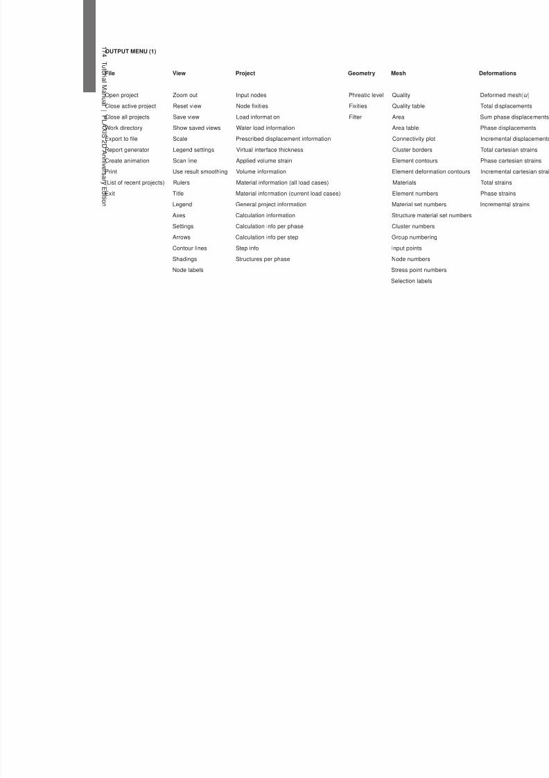
7/21/2019 2DAnniversaryEdition 1 Tutorial
http://slidepdf.com/reader/full/2danniversaryedition-1-tutorial 174/176

7/21/2019 2DAnniversaryEdition 1 Tutorial
http://slidepdf.com/reader/full/2danniversaryedition-1-tutorial 175/176
OUTPUT MENU (2)
Stresses Forces Interface stresses Tools Win
Cross section Axial forces Effective Σ'N Copy Proj
Cartesian effective stresses Shear forces Total ΣN Select points for curves Dup
Cartesian total stresses Bending moments Shear τ N Mesh point selection Clos
Principal effective stresses Table of forces Relative shear τ rel Curves manager Cas
Principal total stresses Maximum shear τ max Table Tile
State parameters Groundwater head Cross section Tile
Pore pressures p active Cross section curves (List
Groundwater flow p water Forces view
Plastic points p steady
Structural forces in volumes
Plastic point history p excess Hint box
Fixed-end anchors Suction Remove annotations
Node to node anchors Suction eff
Wells Plastic points
Drains Table of nodal values
P L A
X I S 2 D
A nni v er s ar y E d i t i on
| T u
t or i al M an u al 1 7 5

7/21/2019 2DAnniversaryEdition 1 Tutorial
http://slidepdf.com/reader/full/2danniversaryedition-1-tutorial 176/176
TUTORIAL MANUAL