2d packet classiﬁcation for internet protocol husni thamrin abstract of master’s thesis academic...

修士論文 2001年度 (平成 13年度)

2D Packet Classification for Internet Protocol

慶應義塾大学大学院政策・メディア研究科

Achmad Husni Thamrin

修士論文要旨　2001年度　（平成13年度）


インターネットの発達により、ルータ内におけるパケット処理が複雑化してきた。ルータは、本来の機能であるパケット転送機能の他に、ファイアウォールやQoSといった様々な機能を持つようになった。パケットのクラス分けは、これらの機能において重要な役割を果たしている。ルータが効率良くクラス分けを行うためには、良いクラス分け手法が必要である。本論文では、ヘッダ中の始点アドレスと終点アドレスを利用した、インターネットにおけ

るパケットの２次元クラス分け手法を提案する。本手法では、あらかじめ、複数の検索面を生成し、その上にフィルタを配置する。目的のフィルタを検索する際は、まず、目的のフィルタが含まれている検索面を探し出す。そして、その検索面内で、目的のフィルタを探し出す。本手法の計算量を解析した結果、最適なフィルタを O(log W )回の検索で発見できること

が判明した。また、データ構造の構築は、O(NW )回の手順で行える。メモリ消費量は最大時に O(N2W )となるが、本手法は最大時になる確率が減少するよう設計した。本手法の評価には、模擬フィルタデータベースを用いた。その結果、メモリ消費量は O(NW )であり、最大時を大きく下回った。

キーワード1. Internet Protocol 2. packet classification 3. filter database 4. firewall5. Quality of Service

慶應義塾大学大学院政策・メディア研究科Achmad Husni Thamrin

Abstract of Master’s Thesis

Academic Year 2001


The Internet’s development has pushed to the more complex processing of Internetpackets in routers. Routers now not only have to forward packets – their main function,but also have to perform other functions such as firewall and Quality of Service functions.The core of these functions is packet classification. Since an Internet router may performseveral classifications for a packet, thus it requires a good packet classification scheme.Packet classification is to classify packets into a flow. Packets are said to match a flow ifthey meet some criterions defined by a rule, thus processed in a similar manner.

This thesis presents a scheme for classifying Internet packets based on two header fieldsof packets, thus called two-dimensional (2D) packet classification. The relevant header fieldsfor this thesis are source and destination addresses. Our scheme solves packet classificationproblem by creating search planes based on filters in a filter database and store the filtersin search planes. Our scheme finds the best matching filter for a packet using a two-stepprocess: find the search plane containing the best matching filter, then find the best matchingfilter in that search plane.

Complexity analysis of our scheme shows that it can search for the best matching filterin O(log W ) time. To build its data structure for a filter database, this scheme requires onlyO(NW ) time. Even though the worst-case memory requirement is O(N2W ), it is designed toreduce the probability of reaching that worst-case. We evaluate our 2D packet classificationscheme by running it using simulated filter databases and the simulation result shows thatthe memory usage tends to be O(NW ), rather than close to the worst-case.

Key Word1. Internet Protocol 2. packet classification 3. filter database 4. firewall5. Quality of Service

Keio University Graduate School of Media and GovernanceAchmad Husni Thamrin

Contents

1 Introduction 11.1 Background . . . . . . . . . . . . . . . . . . . . . . . . . . . . . . . . . . . . 11.2 Packet Classification . . . . . . . . . . . . . . . . . . . . . . . . . . . . . . . 21.3 Research Objective . . . . . . . . . . . . . . . . . . . . . . . . . . . . . . . . 61.4 Organization of Thesis . . . . . . . . . . . . . . . . . . . . . . . . . . . . . . 6

2 Problem Statement and Related Work 72.1 Problem Statement . . . . . . . . . . . . . . . . . . . . . . . . . . . . . . . . 72.2 Related Work . . . . . . . . . . . . . . . . . . . . . . . . . . . . . . . . . . . 8

2.2.1 Scalable High Speed IP Routing Lookup . . . . . . . . . . . . . . . . 82.2.2 Hierarchical Intelligent Cuttings . . . . . . . . . . . . . . . . . . . . 102.2.3 Tuple Space Search . . . . . . . . . . . . . . . . . . . . . . . . . . . . 122.2.4 Fast 2D Classification for Conflict-Free Filters . . . . . . . . . . . . 14

3 2D Packet Classification Scheme 163.1 Binary Search of Prefixes on Multiple Fields . . . . . . . . . . . . . . . . . . 163.2 Searching on Multiple Planes . . . . . . . . . . . . . . . . . . . . . . . . . . 173.3 Filter Search Plane . . . . . . . . . . . . . . . . . . . . . . . . . . . . . . . . 183.4 Algorithm to Search for FSP . . . . . . . . . . . . . . . . . . . . . . . . . . 213.5 Searching for Filters in an FSP . . . . . . . . . . . . . . . . . . . . . . . . . 243.6 Storing Filters in a Search Plane . . . . . . . . . . . . . . . . . . . . . . . . 253.7 Building the Database Structure . . . . . . . . . . . . . . . . . . . . . . . . 273.8 Dealing with Wildcard Filter Problem . . . . . . . . . . . . . . . . . . . . . 27

4 Simulation 324.1 The Implementation Data Structure . . . . . . . . . . . . . . . . . . . . . . 324.2 Simulation Filter Database Design . . . . . . . . . . . . . . . . . . . . . . . 34

4.2.1 Cross-producting prefixes . . . . . . . . . . . . . . . . . . . . . . . . 364.2.2 Random prefixes . . . . . . . . . . . . . . . . . . . . . . . . . . . . . 36

4.3 Cross-product Filter Database Result . . . . . . . . . . . . . . . . . . . . . 384.4 Random Non-wildcard Filter Database Result . . . . . . . . . . . . . . . . . 39

4.4.1 Build time . . . . . . . . . . . . . . . . . . . . . . . . . . . . . . . . . 394.4.2 Memory requirement . . . . . . . . . . . . . . . . . . . . . . . . . . . 39

4.5 Random Wildcard Filter Database Result . . . . . . . . . . . . . . . . . . . 434.6 Memory Requirement of the Scheme in Section 3.1 . . . . . . . . . . . . . . 45

i

5 Analysis and Evaluation 465.1 Effect of Duplicated Prefixes . . . . . . . . . . . . . . . . . . . . . . . . . . 465.2 Memory Requirement . . . . . . . . . . . . . . . . . . . . . . . . . . . . . . 47

5.2.1 Non-wildcard filter database . . . . . . . . . . . . . . . . . . . . . . . 475.2.2 Adding wildcard filters . . . . . . . . . . . . . . . . . . . . . . . . . . 48

5.3 Build Time . . . . . . . . . . . . . . . . . . . . . . . . . . . . . . . . . . . . 505.4 General Evaluation . . . . . . . . . . . . . . . . . . . . . . . . . . . . . . . . 50

6 Conclusion 526.1 Summary . . . . . . . . . . . . . . . . . . . . . . . . . . . . . . . . . . . . . 526.2 Future Work . . . . . . . . . . . . . . . . . . . . . . . . . . . . . . . . . . . 53

Acknowledgments 54

Bibliography 55

ii

List of Figures

1.1 Typical packet-processing flow in an IP router. . . . . . . . . . . . . . . . . 21.2 Conceptual model of packet classification. . . . . . . . . . . . . . . . . . . . 21.3 A filter database. . . . . . . . . . . . . . . . . . . . . . . . . . . . . . . . . . 31.4 Routing table of a router in Telstra Network. . . . . . . . . . . . . . . . . . 41.5 Active BGP entries in Telstra Network. . . . . . . . . . . . . . . . . . . . . 41.6 BGP update in Telstra Network. . . . . . . . . . . . . . . . . . . . . . . . . 41.7 BGP table growth - projections. . . . . . . . . . . . . . . . . . . . . . . . . 5

2.1 Hash tables for prefix lengths. . . . . . . . . . . . . . . . . . . . . . . . . . . 82.2 Binary search on hash tables. . . . . . . . . . . . . . . . . . . . . . . . . . . 92.3 Binary search on trie levels. . . . . . . . . . . . . . . . . . . . . . . . . . . . 92.4 Geometrical representation of seven filters. . . . . . . . . . . . . . . . . . . . 112.5 A possible tree for filters in Figure 2.4. . . . . . . . . . . . . . . . . . . . . . 112.6 Illustration of markers and precomputation. . . . . . . . . . . . . . . . . . . 132.7 Illustration of search strategy. . . . . . . . . . . . . . . . . . . . . . . . . . . 142.8 Two conflicting filters. . . . . . . . . . . . . . . . . . . . . . . . . . . . . . . 14

3.1 Entries for 2D filters using [8] algorithm. . . . . . . . . . . . . . . . . . . . 173.2 A 2D filter and its search plane. . . . . . . . . . . . . . . . . . . . . . . . . . 183.3 Filter overlap is not possible for prefix form fields. . . . . . . . . . . . . . . 183.4 Three filters and search planes. . . . . . . . . . . . . . . . . . . . . . . . . . 203.5 Cases of FSP of two filters. . . . . . . . . . . . . . . . . . . . . . . . . . . . 203.6 FSPs occupy a diagonal of 2D Tuple Space. . . . . . . . . . . . . . . . . . . 223.7 Filters that can be stored in an FSP. . . . . . . . . . . . . . . . . . . . . . . 243.8 Expanding FSPn in FSPm to find filters. . . . . . . . . . . . . . . . . . . . 263.9 FSPn and FSPm store F1. . . . . . . . . . . . . . . . . . . . . . . . . . . . 273.10 A wildcard filter in filter database. . . . . . . . . . . . . . . . . . . . . . . . 28

4.1 Data structure for a filter. . . . . . . . . . . . . . . . . . . . . . . . . . . . . 324.2 Marker for a filter. . . . . . . . . . . . . . . . . . . . . . . . . . . . . . . . . 334.3 An FSP. . . . . . . . . . . . . . . . . . . . . . . . . . . . . . . . . . . . . . . 334.4 Marker for an FSP. . . . . . . . . . . . . . . . . . . . . . . . . . . . . . . . . 334.5 Data structure of FSP hash key. . . . . . . . . . . . . . . . . . . . . . . . . 344.6 Data structure of filter hash key. . . . . . . . . . . . . . . . . . . . . . . . . 344.7 AS border routers. . . . . . . . . . . . . . . . . . . . . . . . . . . . . . . . . 354.8 Time to build the data structure for all filter database. . . . . . . . . . . . . 39

iii

4.9 Filters in structure for all combinations. . . . . . . . . . . . . . . . . . . . . 404.10 Filters of AS 701 pairing with other top 5 of prefix and level ASes. . . . . . 404.11 Filters of AS 701 pairing with other top 5 of duplicated prefix and the per-

centage ASes. . . . . . . . . . . . . . . . . . . . . . . . . . . . . . . . . . . . 414.12 Filters of AS 4787 pairing with other top 5 of prefix and level ASes. . . . . 414.13 Filters of AS 4787 pairing with other top 5 of duplicated prefix and the

percentage ASes. . . . . . . . . . . . . . . . . . . . . . . . . . . . . . . . . . 414.14 Filters of AS 8010 pairing with other top 5 of prefix and level ASes. . . . . 424.15 Filters of AS 8010 pairing with other top 5 of duplicated prefix and the

percentage ASes. . . . . . . . . . . . . . . . . . . . . . . . . . . . . . . . . . 424.16 Filters of AS 9796 pairing with other top 5 of prefix and level ASes. . . . . 424.17 Filters of AS 9796 pairing with other top 5 of duplicated prefix and the

percentage ASes. . . . . . . . . . . . . . . . . . . . . . . . . . . . . . . . . . 434.18 Adding wildcard filters created from AS 701. . . . . . . . . . . . . . . . . . 434.19 Adding wildcard filters created from AS 4787. . . . . . . . . . . . . . . . . . 444.20 Adding wildcard filters created from AS 8010. . . . . . . . . . . . . . . . . . 444.21 Adding wildcard filters created from AS 9796. . . . . . . . . . . . . . . . . . 444.22 Filters of AS701 using the scheme in Section 3.1. . . . . . . . . . . . . . . . 45

5.1 F11 is stored in FSP (F11) and FSP (F12). . . . . . . . . . . . . . . . . . . 475.2 Top series of top 4 ASes. . . . . . . . . . . . . . . . . . . . . . . . . . . . . . 48

iv

List of Tables

2.1 Comparison of worst-case lookup time and space complexities for 2-D packetclassification. . . . . . . . . . . . . . . . . . . . . . . . . . . . . . . . . . . . 15

3.1 FSP and its contained filters of Figure 3.4. . . . . . . . . . . . . . . . . . . . 203.2 Filter database to show the case of Figure 3.5 (d). . . . . . . . . . . . . . . 21

4.1 ASes for cross-product filter databases. . . . . . . . . . . . . . . . . . . . . . 364.2 AS ranked by number of prefixes. . . . . . . . . . . . . . . . . . . . . . . . . 364.3 AS ranked by maximum prefix level. . . . . . . . . . . . . . . . . . . . . . . 374.4 AS ranked by duplicated prefixes. . . . . . . . . . . . . . . . . . . . . . . . . 374.5 AS ranked by percentage of duplicated prefixes. . . . . . . . . . . . . . . . . 374.6 Filters in structure of cross-product filters. . . . . . . . . . . . . . . . . . . . 384.7 Percentage of filters in structure of cross-product filters. . . . . . . . . . . . 39

5.1 Distinct and duplicated prefixes of ASes in filter databases. . . . . . . . . . 495.2 Distinct and top level prefixes of AS . . . . . . . . . . . . . . . . . . . . . . 50

6.1 Our scheme and other 2D packet classification schemes. . . . . . . . . . . . 53

v

List of Algorithms

1 Storing markers of FSP . . . . . . . . . . . . . . . . . . . . . . . . . . . . . 232 Binary search to find the FSP containing the best matching filter. . . . . . 233 Storing filters in an FSP. . . . . . . . . . . . . . . . . . . . . . . . . . . . . . 254 Searching for the BMF of a packet. . . . . . . . . . . . . . . . . . . . . . . . 255 Follow markers to find filters. . . . . . . . . . . . . . . . . . . . . . . . . . . 296 Find all filters in FSPl to be stored in FSPs. . . . . . . . . . . . . . . . . . 307 Build database structure for a filter database. . . . . . . . . . . . . . . . . . 31

vi

Chapter 1

Introduction

1.1 Background

The Internet is a collection of interconnected hosts. These hosts are interconnected usinglinks. Some hosts can only act as the termination point of data (end-hosts), while the otherscan serve as the intermediaries for end-hosts (routers). Hosts on the Internet communicateusing Internet Protocol (IP) where data are exchanged in the form of IP datagram. IPdatagrams packets travel from the source host to their destination through routers, androuters are responsible to forward these datagrams to reach their final destination.

The capability to forward packets is a requirement of every IP router [2]. An IP routermay also do additional processing on incoming packets. The most common process addedto an IP router was packet filtering for security purposes. Now, however, some IP routersperform many new additional processing to the packets, such as delivery guarantees interms of bandwidth, delay, and jitter, and statistics for billing purposes. All these processesrequire IP router to classify packets into a flow. Packets are said to match a flow if theymeet some criterions defined by a rule, thus processed in a similar manner.

The Internet’s development has pushed to the more complex packet-processing in IProuters. The complexity is measured by line speed, the number of packet processing, andthe difficulty level of each packet processing that must be supported by an IP router.Generally, the complexity of packet processing in a router corresponds to router’s locationin the Internet. If a router is located on the backbone of the Internet, packet processing inthat router tends to be more complex than another router located on the leaf of Internet.

Figure. 1.1 shows the typical processing of packets inside the router. An incoming packetis first processed by firewall module to know whether the router can accept the packet orhas to drop it. If the router accepts the packet, QoS (Quality of Service) module processesthe packet to know whether the corresponding flow of the packet still conforms to its QoSspecification. Assuming the packet is not dropped, it is then processed by packet forwardingmodule to forward the packet to the correct gateway to destination.

Now that the router knows the next-hop gateway – and the outgoing interface – of thepacket, once again firewall and QoS modules process the packet. Firewall module decideswhether the packet can be forwarded through the outgoing interface. If it can be forwarded,QoS module performs prioritization, packet shaping, etc., so packets’ flow conforms to itsspecification. This is an illustration of how packets get processed by many modules in an

1

CHAPTER 1. INTRODUCTION 2

Firewall

QoS

Firewall QoS

Billing Packet

Forwarding

Incoming Packet

Outgoing Packet

Figure 1.1: Typical packet-processing flow in an IP router.

dst addr

src addr

proto dst port

src port

data

packet �

F1

F2

F3

Fn

...

...

...

Filter database

packet classification

algorithm �

matched filter

Figure 1.2: Conceptual model of packet classification.

IP router.

1.2 Packet Classification

The above mentioned packet processings have something in common, they have a set ofrules and they match incoming packets to the rules to find which rule(s) match(es) thepacket. This common function is usually called packet classification. Figure 1.2 illustratesthe conceptual model of a packet classification.

Packet classification function has three components: a packet, a filter database, and analgorithm to classify packets. A Packet is the IP datagram to be matched with filters in thefilter database. The packet has several properties that are relevant to classification: sourceand destination addresses, type-of-service, length, etc.

Filter database is a collection of filters (also called rules), and each filter consists ofseveral fields and an action. Each field of a filter is associated to a certain property ofIP packet, usually to a packet header field. Each field can be in the form of single value(e.g. 23), range (e.g. 0–1023), prefix (e.g. 203.178.143/24), or wildcard (matches all values).

A packet property matches to its corresponding filter field if the value of that property


is contained within the value range of the filter field. A packet matches to a filter if allproperties of the packet match to the corresponding fields of the filter. When this happens,packet is classified into the flow defined by the filter, and will be treated according to theaction of the filter.

As an example, filter database in Fig. 1.3 has three filters. This filter database de-fines three flows. Assuming we have a TCP packet whose source address is 202.249.47.142,destination address: 203.178.143.121, source port: 40123, and destination port: 22. Thispacket matches to the upper filter, thus it is permit-ted to enter the router. However, if thepacket is an ICMP packet whose source and destination addresses are 202.249.47.142 and203.178.148.24, then it matches to the middle filter. Therefore, it is deny-ed from enteringthe router.

tcp src 202.249.47/24 port * dst 203.178.142/23 port 20–23 permitip src 202.249/17 dst 203.178.148/25 denyip src * dst * permit

Figure 1.3: A filter database.

Packet classification algorithm performs the matching between IP packet and the filtersto find which filter matches the packet. A naive algorithm would be to compare the packetwith each filter in filter database, from top to bottom, until the algorithm finds a matchedfilter. However, this algorithms’ speed depends linearly to the number of filters in database.From the illustration of Figure 1.1, it is clear that a router may invoke packet classificationfunction – thus, the algorithm – several times, each from different modules. Therefore,packet classification algorithm should be fast enough to allow the algorithm being executedseveral times and still can forward packets at line speed.

The complexity of packet classification problem depends on the number of filter fieldsand the number of filters that must be supported. If the number of filter fields (usuallycalled dimensionality) becomes larger, then the problem becomes more complex. This alsoapplies to the number of filters in filter database.

Packet classification can be categorized as layer 3 or layer 4 classification, dependingon the fields of filters. Filters of layer 3 classification uses IP address fields or other packetheader fields that are relevant for processing at the Internet Layer of TCP/IP protocolstack. If classification includes other fields that are only relevant to UDP and TCP, then itis called layer 4 classification.

Packet forwarding is an example of layer 3 classification. Filters for packet forwarding,the routing/forwarding table, have only one field that corresponds to destination address ofan IP packet. The action of these filters is the next hop gateway for the matching packet.Fig. 1.4 shows a portion of BGP (Border Gateway Protocol) routing table of a router inTelstra Network, which contains the routing table of the whole Internet. Data from TelstraNetwork Australia [1] at December 5, 2001 16:03 (GMT+10) showed that the current BGProuting table holds about 100 thousand active entries (Figure 1.5) and updated at the rateof 550 times per hour on average (Figure 1.6). These data show that while packet forwardingonly has one dimension, it is required to support large database and fast update.

Firewall and QoS functions – in general – are layer 4 classification since they tend to useport fields for their filter databases. Firewalls are used not only to prevent or allow traffic


Network

3.0.0.0

4.18.12.0/22

Next Hop

202.84.219.194

203.50.126.70 ...

167.202.192.0/19

167.203.0.0

203.2.135.0

203.2.142.0

...

203.14.6.7

203.14.0.4

...

202.84.219.194

202.84.219.193 ...

Figure 1.4: Routing table of a router in Telstra Network.

Figure 1.5: Active BGP entries in Telstra Network.

Figure 1.6: BGP update in Telstra Network.


from and to certain hosts, but also from and to certain hosts using certain applications,indicated from the protocol type and port fields. QoS function may the same port fields asfirewall with the purpose of prioritization, traffic shaping, etc.

As of now, it is not clear how many filters defined in the largest firewall database on theInternet, since network administrators do not want to expose their filters due to securityreasons. Firewall database obtained by others in packet classification field are less than2000 filters [3][6][7]. No papers stated that they are using filter databases for QoS function.Despite the difficulties of obtaining real-life filter databases, it is safe to assume that filterdatabases for firewall and QoS are like that of BGP routing table for the IP address fields,while the port fields depend on the popular applications on the Internet.

BGP routing table is an indicator to estimate the complexity for IP address basedpacket classification. Each entry in BGP routing table has information about its originatingAS (Autonomous System). An Autonomous System is defined as a group of IP networksoperated by one or more network operators that has a single and clearly defined externalrouting policy and expressed as AS Number. However, owing to dropping price of telecom-munication lines, many enterprises start to have connectivity to several network operators(multi-homing network) and they apply for their own AS number [5]. This fact practicallymeans that an AS is likely to also have a policy for its firewall and QoS functions because anenterprise tend to have a policy for such functions. Therefore if BGP routing table becomeslarger, then we would likely to find larger filter database.

Figure 1.7: BGP table growth - projections.

In the future, BGP routing table will expand further due to increasing number of multi-homing networks [5]. Figure 1.7 shows the projection of BGP routing growth [5]. The upperand lower the projection based on the past six months and two years trends, respectively.This growth means that more IP prefixes are being advertised to the Internet. This wouldlikely be followed by the increase of filter database size for firewall and QoS functions,mainly because their filter databases have to reflect the increase of IP prefixes on theirIP address fields: source and destination addresses. Due to this projection, it is importantto have two-dimensional packet classification that is capable of handling many source and


destination address filters.

1.3 Research Objective

The previous sections showed that IP routers might execute packet classification severaltimes to process an IP packet. Because of this, then it is important to have good packetclassification function on IP routers. Given the importance of packet classification and theoutlook of BGP routing expansion, the objective of this research is to find a good schemefor classifying two-dimensional –source and destination– filters.

1.4 Organization of Thesis

This thesis consists of six chapters. The next chapter states the problem formally and de-scribes related work on this field. Chapter 3 explains a two dimensional packet classificationscheme, which is the idea of this thesis. Chapter 4 presents implementation and simulationresult. In Chapter 5 we analyze and evaluate our scheme based on the design and simulationresults, and we give summary and conclusion in the final chapter.

Chapter 2

Problem Statement and RelatedWork

2.1 Problem Statement

Packet classification is looking at K fields in the headers of each packet that are relevant toclassification. Suppose we have a packet P and a filter F . A filter F is a K tuple (F [1], F [2],. . . , F [K]) where each F [i], 1 ≤ i ≤ K, is a filter for the corresponding field in a packet,which can be a single value, a variable length prefix bit string, or a range. Variable lengthprefix bit string is mostly used for address fields while range is usually used for port fields.Each filter F has an action that is associated with that filter. For example, a filter mightbe used to block or accept a packet, or even divert it as we see in some filter applicationssuch as ipfw of FreeBSD.

Each field in filter F is compared to the corresponding field of packet P . Let P [i] is thecorresponding field of F [i]. A field F [i] matches P [i] if the value of P [i] is within the rangeof F [i]. A filter F is said to match a packet P if all fields of F matches the correspondingfield of P , i.e. F [i] matches P [i], 1 ≤ i ≤ K. As an example, let (167.205/16, 202.249.47/24)be a filter of source and destination IP addresses. This filter matches an IP packet withsource 167.205.22.108 and destination 202.249.47.142, but not an IP packet whose sourceand destination are 202.249.47.133 and 203.178.143.1.

A filter database consists of N rules F1, F2, ..., FN where each filter has K distinctfields. In a filter database, there is a possibility that two or more filters match a given packetso we have to have a tie breaking mechanism to define the best matching filter. To simplifythe problem, let each filter in a filter database has an associated cost, if there is more thanone rule match a given packet then we define the best matching filter as the least-cost filter.In practice, a filter database is usually indexed linearly and we can use the index number asthe cost of the filter. A filter denoted as Fn has n as its’ index number. As an example, if ina filter database, F2 and F6 match a packet P , then we say that F2 is the best matchingfilter for packet P .

This research is on the two-dimensional case of packet classification (K = 2). Packetheaders that are relevant for this research are source address and destination address. SinceIP addresses are often expressed in the form of prefix, this research assumes that every filterin the filter database can only have that form.

7

CHAPTER 2. PROBLEM STATEMENT AND RELATED WORK 8

Length Hash

4

8

10

0101

01010110 01101011

0111010110

Hash Tables

Figure 2.1: Hash tables for prefix lengths.

2.2 Related Work

There are many publications that are related to packet classification problem. This sectionsummarizes four works by others. This section is closed with a table showing the comparisonof several packet classification schemes.

2.2.1 Scalable High Speed IP Routing Lookup

Waldvogel et.al. [8] describes a new algorithm for best matching prefix using binary searchon hash tables organized by prefix lengths. This algorithm requires a worst-case oflog2(addressbits) hash lookups, thus it scales very well.

There are three significant ideas of this algorithm: using hashing to check whether anaddress D matches any prefix of a particular length; binary search to reduce the number ofsearches from linear to logarithmic; and precomputation to prevent backtracking in case offailures in the binary search of range.

Hashing idea is to look for all prefixes of a certain length L using hashing and usemultiple hashes to find the best matching prefix, starting with the largest value of L andworking backward.

As an example, consider a routing table of four prefix entries, each with prefix length of4, 8, 8, and 10. Each of the entries would be stored in a hash table that corresponds to its’prefix length (Figure 2.1). The hash tables are stored as a sorted array, so for this example,the array has three entries.

Searching for address D, we walk through each hash table in that array starting fromthe largest value l, i.e. 10 on the example, extracting the first l bits of D to get its prefixof D. We then search the hash table using that prefix as the key. If we found a prefix, thenwe have found the best matching prefix (BMP) and the search terminates; otherwise if wefound nothing, we move to the next entry of the array. As we see here, the worst-case searchtime of this algorithm is O(Wdist) hash lookups, Wdist is the distinct prefix lengths in thedatabase, which is less than W (bit width of the address).

A better strategy for this search is to use binary search on that array. To do this, weneed to put markers in the tables corresponding to shorter lengths to point to prefixes ofgreater lengths. These markers direct binary search to look for matching prefixes of greaterlength. This way, the number of hashes is cut down to O(log2Wdist). Searching for an IPv4


1

2

3

L

P1=0

P2=00

P3=111 111

00

0

11

(a) (b) (c)

Binary Search Hash Tables Hash Tables with Marker

Figure 2.2: Binary search on hash tables.

Incr

easi

ng P

refix

Len

gth

Binary Search �

Trie Structure �

Figure 2.3: Binary search on trie levels.

address would require 5 hash accesses in the worst case.To illustrate the binary search strategy, suppose we have three prefixes P1 = 0, P2 = 00,

P3 = 111. Storing the prefixes in hash tables and sorting the array, we have Figure 2.2 (b).If we search for 111, binary search (a) would start at the middle of the hash table and searchfor 11 in the hash table containing P2. This search would fail and have no pointer that itshould search in the longer prefix tables to find the BMP. To correct the search, we need toput the marker for prefix P3 in this table, thus the lookup for 11 would succeed and binarysearch would know that it should search for a match in the longer prefix table.

The hash tables containing prefixes and markers can be thought as a trie where eachhash table is a level of a trie that corresponds to nodes of a certain prefix length (Figure 2.3.Binary search in this trie starts on the median level of the trie and depending on the resultof hash lookup on that level, the search will continue to the level of shorter or longer prefixlength.

Another effect of using binary search on trie levels is the number of markers is reducedto at most log2W markers per real prefix. This reduction is achieved because it suffices toplace markers at all levels in L that could be visited by binary search when looking for anentry whose BMP is P.


A naive implementation of this algorithm will take linear time. Markers, while can pointto the BMP, they can also cause the search to follow false lead, which may fail. When thishappens, we would have to modify the binary search to backtrack and search the upper halfof the level of failure, and that would lead to linear time.

To avoid the backtracking problem, we need use precomputation when inserting markers.Suppose we insert a marker M to the hash table, M would have to record the best matchingprefix of the marker (M.bmp). With this variable, now the binary search remembers thevalue of M.bmp whenever a lookup produces a match. If the search in the lower half producesa failure, search procedure doesn’t need to backtrack, since it remembers the best matchingprefix from M.bmp.

Waldvogel et.al. also shows some refinements to the scheme explained above to reducethe average number of hash computations. These are asymmetric binary search and mutatingbinary search. Both optimizations exploit the structure of the data set. Interested readerscan read [8] for the details.

2.2.2 Hierarchical Intelligent Cuttings

Gupta and McKeown [3] uses heuristics to solve k-dimensional packet classification prob-lem. Their approach focuses on the practical implementation of classification with real-lifefilter database. The approach, called HiCuts (hierarchical intelligent cuttings), attempts topartition the search space in each dimension, guided by simple heuristics that exploit thestructure of filter database.

The HiCuts algorithm builds a decision-tree data structure by carefully preprocessingthe filter database. Each time a packet arrives, the classification algorithm traverses thedecision tree to find a leaf node, which stores a small number of rules. A linear search ofthese rules produces the matching filter.

During the preprocessing, HiCuts creates internal nodes of the decision tree. For eachinternal nodes v, HiCuts associates some properties

• A box B(v), which is a k-tuple of ranges or intervals.

• A cut C(v), the dimension d where B(v) is cut, and np(C), the number of equalintervals B(v) is cut into in dimension d. This cut forms the children of v.

• A set of filters R(v), which is a subset of filters in the filter database that collides withv.

HiCuts starts with a root node v and store all filters R(v) in that node. It then cuts thenode in dimension d into np(C) equal intervals using heuristics that selects both parameters.Node v now has np(C) children nodes and HiCuts stores subsets of R(v) in each childrennodes. The algorithm partitions every nodes of the tree until the number of filters thatcollides with the node doesn’t exceed a threshold, which is called binth. Nodes having nomore than binth rules form the leaf nodes of the decision tree.

Figure 2.4 illustrates the geometrical representation of a two-dimensional filter database.Figure 2.5 shows a possible tree for the database. Each ellipse denotes an internal node vwith a triplet (B(V ), dim(C(v)), np(C(v))). Each rectangle is a leaf node that contains therules. This example uses 2 as its binth.

The preprocessing algorithm of HiCuts uses four heuristics to partition nodes:


0 �

0 �

255 �

255

X

Y

R1

R2

R3

R7

R6

R4

R5

Figure 2.4: Geometrical representation of seven filters.

(256 * 256, X, 4)

R1 R2

(64 * 256, X, 4)

R1 R2

R1 R2

R1 R2

R1 R2

Figure 2.5: A possible tree for filters in Figure 2.4.

• A heuristic that chooses a suitable np(C). A large value of np(C) will decrease thetree’s depth at the expense of increased storage.

• A heuristic that chooses the dimension to cut along at each internal node.

• A heuristic that maximizes the reuse of child nodes.

• A heuristic that eliminates redundancies in the tree.

All these heuristics are combined to create the “best” decision tree for the filter databaseand tuning parameters for these heuristics would possibly create different trees.

Tests on this algorithm use two-dimensional filter database created from publicly avail-able routing tables. For higher dimensions classification, tests are performed using filterdatabase obtained from ISP (Internet Service Provider) and enterprise networks. The num-bers of filters in those databases are between 100 and 1,733.

The results of the tests showed that HiCuts algorithm performed well on the availablefilter database. Worst case search was only 20 memory accesses (200 ns for 10ns SDRAMmemory). The memory requirement was small compared to its theoretical worst case. It is


important to consider the preprocessing time for this algorithm. The worst preprocessingtime was 50 seconds on Pentium-II 333-MHz for a database containing less than 1,000 filters.

2.2.3 Tuple Space Search

Another packet classification scheme that uses hashing is Tuple Space Search [6]. This re-search is motivated by the observation that while filter databases contain many differentprefixes or ranges the number of distinct prefix lengths tends to be small. This observationis backed by empirical study of some industrial firewall database. Knowing this, Srini-vasan et.al [6] defined a tuple for each combination of field length and called the resultingset tuple space. Each tuple has a known set of bits in each field, therefore we can create ahash key by concatenating these bits in order , which can then be used to map filters ofthat tuple into a hash table.

Tuple Space Search (TSS) is a general packet classification, however the research focusedon 5-dimensional filters for the experiments: IP source, IP destination, protocol type, sourceport number, and destination port number.

TSS defines a tuple T as a vector of K lengths, K is the number of fields for filtering. Forexample, [8, 16, 8, 0, 16] is a 5-dimensional tuple, whose IP source field is an 8-bit prefix, IPdestination field is a 16-bit prefix, and so on. A filter F belongs or maps to tuple T if the ithfield of F is specified to exactly T [i] bits. For example, 2-dimensional filters F1 = (01∗, 111∗)and F2 = (11∗, 010∗) both map to the tuple [2, 3].

Tuples require every fields of a filter to be specified as a length. While IP addresses arealways specified using prefixes, port numbers are not. Port numbers are usually specifiedusing ranges, e.g. [0, 1024]. TSS gets around this requirement by using nesting level andRangeId each to simulate prefix length and prefix of IP addresses. For example, we havethree ranges: F1 = [0, 65535], F2 = [0, 1023], and F3 = [1024, 65535]. F1 has nesting level of0 and RangeId of 0. F2 and F3 are nested from F1, thus their nesting level is 1, and theyreceive RangeId of 0 and 1, respectively.

With the get around explained above, each filter can now be mapped to a particulartuple T in a hash table Hashtable(T ) with the concatenated prefix-es and RangeId-es asits hash key. Probing a tuple T involves concatenating the required number of bits from thepacket P as specified by T and then doing a hash in Hashtable(T ).

Searching for a matched filter for a given packet P is performed by linearly probes allthe tuple in the tuple set. If more than one matching filters were found, TSS picks the leastcost filter. The search cost is proportional to m, the number of distinct tuples, which can beup to N , the number of filters in database. However, the previous observation showed thatN tends to be much larger than m. Update cost (inserting and deleting a filter) for tuplespace search is also small, only one hash access. Thus, we can say that tuple space searchperforms much better than linear search.

Srinivasan et.al. [6] shows several improvements for the basic tuple space search. Twoof them are summarized next: Tuple Pruning and Rectangle Search.

Tuple Pruning is motivated by the observation that in real filter databases there seem tobe very few prefixes of a given address. For example, in Mae-East prefix database there is noaddress D has more than 6 matching prefixes. If a 2-dimensional filter is formed from thatdatabase, then if we first find the longest destination match and the longest source match,there are only at most 6 x 6 = 36 possible tuples that are compatible with the individual


0 �

1

2 �

3 �

4 �

5 �

Z1 �

Z �

F1 F2 F3 F4 F

Markers F4 F3 F2 F1 Z1

Filters F = 101*, 1110* Z �

= 1*, 1*

101*, 111* 101*, 11* 101*, 1* 101*, * 1*, *

Figure 2.6: Illustration of markers and precomputation.

destination and source matches. This is very small compared to the maximum number ofpossible tuples for IP source-destination pair, which is 36 x 36 = 1024.

For instance, consider a 2-dimensional filter database for source S and destination Daddresses. Suppose D = 1010∗, and all the filters whose destination is a prefix of D belongto tuples [1, 4], [1, 1], and [2, 3]. Then, the tuple list of D contains these 3 tuples. Similarly,suppose S = 0010∗, and all filters whose source is a prefix of S belong to tuples [2, 4], [1, 1],and [2, 5].

Searching for the matching filter for a packet P computes the longest matching prefixPD and PS for destination and source addresses of P . The next step is to take the tuple listsstored with PD and PS, find their common intersection, and probe into that intersection.If PD = D and PS = S as above, the intersection list only includes [1, 1], thus we onlyprobe into one tuple.

Rectangle Search is an improvement from the basic tuple space search for 2-D filterdatabase. Rectangle Search works to cut the search time by using precomputation andmarkers. Search time is now down from W 2 hash accesses of basic tuple space search into2W accesses, W is the bit width of address. [6] also shows that this algorithm is optimalfor 2-D filter database.

When a filter is added to the database, it leaves a marker at all the tuples to its leftin its row. So a filter in the tuple [i, j] leaves a marker in tuples [i, j − 1], [i, j − 3], . . . ,[i, 1]. Each filter (or marker) also precomputes the least cost filter matching it from amongthe tuples above it in its column. That is, a filter (or marker) in tuple [i, j] precomputesthe least cost filter matching it from the tuples [i− 1, j], [i− 2, j], . . . , [1, j]. This is themarking and precomputation strategy for rectangle search.

Figure 2.6 shows an example of precomputation and markers, using two filters F andZ. The marker F2 precomputes the best matching filter among the entries in the columnabove it, which in this example is Z.

The search strategy for this algorithm starts by probing the lower-left tuple, namely,[W, 1]. At each tuple, if the probe returns a match, the search moves to the next tuple in theright. If there is no match, the search moves up one row in the same column (Figure 2.7).When a match is found, it is an indication that there is a filter on the right of the currenttuple, thus it is not necessary to probe into the tuples above the current one. However,in case of no match, then there is no filter in the tuples on the right, therefore the search


Match

No Match r

c

T

r-1

c

T

T'

r �

c+1

T T'

Figure 2.7: Illustration of search strategy.

can eliminate the tuples on that row. The search terminates when we reach the rightmostcolumn or the first row.

This strategy requires at most 2W − 1 probes since there are W rows and W columnsand requires O(NW ) memory. However, if we want to trade speed with memory, we canget O(N

√W ) memory for for 3W number of hash accesses in the worst case.

2.2.4 Fast 2D Classification for Conflict-Free Filters

Warkhede, et.al. [9] shows that for two-dimensional filter database, the search speed can beimproved to O(log2W ) in the worst case if there is no conflicting filter in the filter database.

Warkhede et.al. define the best matching filter for a packet P as the matching filter thatis not less specific than any other matching filter. This definition differs than the one insection 2.1 that uses filter index number as the tie-breaking mechanism.

Let filters F1 and F2 are two matching filters for packet P . The two filters conflict ifsome fields of F1 are more specifics, i.e. have longer prefix, than F2. Figure 2.8 shows anexample two conflicting filters. In this case, the classification faces ambiguity because noneof the two filters meets the definition of the best matching filter. To eliminate ambiguity,the classification uses conflict resolution filters proposed by Hari et.al. [4] that introducesa new filter that covers the conflicting area of the filters (F3 in Figure 2.8).

F1

F2 F3 Filter F1 F2

F3

Source Prefix 10* 1011*

1011*

Destination 0101* 01*

0101*

source address

destination address

Figure 2.8: Two conflicting filters.


After resolving filter conflicts, this algorithm maps each filter to its tuple space andstored in a hash table. Each filter can create markers in the same row to its left, which issimilar to [6]. In order to perform binary search on column, one half of the tuple space has tobe eliminated at a time. If the hash probe returns no match, we can eliminate the entire righthalf of tuple space. On the other hand, if there is a match, then the entire left half of tuplespace can be eliminated. This elimination is possible because there is no conflicting filterin database. Thus, we can do binary search on columns. If we do linear search on the rows,then hash probe would take O(W log W ) in the worst case and it requires O(NW log W )memory.

All filters in the same column have the same prefix length on one dimension. If weconcatenate this prefix with the prefix of the other dimension, then we can determinewhether there is a matching filter in the column by using best matching prefix lookup. Ifusing [8], then only O(log W ) hash probes are required for each column search. Thus, searchis now O(log2W ) and requires O(N log2W ) memory.

Table 2.1 compares the complexities of several two-dimensional packet classificationschemes.

Table 2.1: Comparison of worst-case lookup time and space complexities for 2-D packetclassification.

Scheme Lookup time Memory usageTuple space search O(W 2) O(N)Rectangle search O(W ) O(NW )Pruned tuple space O(W 2) O(N)Grid of tries O(W ) O(NW )Cross-producting O(log W ) O(N2)Fast-2D O(log2W ) O(N log2W )

Chapter 3

2D Packet Classification Scheme

As stated in the Chapter 1, two-dimensional packet classification for source and destinationIP addresses is important because of the expected expansion of the Internet and the IPaddress usage. This expansion would lead to large filter databases to be installed in manyrouters. At the same time, routers need to process incoming packets faster than the linespeed of their interfaces. This is the objective of any packet classification schemes, includingthe algorithm that will be described in this chapter: to do faster packet classification forlarger filter database.

This chapter explains a scheme to perform two-dimensional packet classification. Thebasic idea of our scheme is to create many search planes and store filters in search planes.Using this idea, we can have a fast packet classification while reducing the probability ofmemory explosion.

3.1 Binary Search of Prefixes on Multiple Fields

The Scalable High Speed IP Routing Lookup [8] results in a logarithmic scale of the addressbit width, O(log W ), for routing lookup, which is a one-dimensional packet classification.The result is considerably fast, it requires only 5 hash accesses for IPv4 address, comparedto 32 memory accesses when using radix trie. If we use perfect hash algorithm, then onehash access requires only one memory access, thus [8] is more than 6 times faster thanradix trie.

The result makes it tempting to apply the algorithm to perform packet classification onmore than single fields. It would make the search complexity to be O(d log W ), where d isthe number of fields for classification. However, the algorithm would require O(Nd) memoryin the worst case and would easily reach that worst case.

Consider an example of a 2D packet classification using this algorithm. To find the bestmatching filter for a packet P using [8], we have to perform the algorithm twice: search forthe best matching prefix (BMP) on the source address, BMPsrc, then search for the BMPon the destination address, BMPdst, based on the value of BMPsrc. One way to do thisis by concatenating BMPsrc to the destination prefix to search for BMPdst, similar to theone performed by [9]. The result of this search is the best matching filter for packet P andwe can get it in O(2 log W ) time.

Suppose we have a 2D filter database. We first store an entry, srcpref, in HashTable(src)

16

CHAPTER 3. 2D PACKET CLASSIFICATION SCHEME 17

for each filter, based on the source prefix of that filter. One can see that an entry mightrepresent more than one filter. For example, we have two filters F1 = (S1, D1) and F2 =(S2, D2). If S1 is a prefix of S2, i.e. S1 = S2 ·A, where “·” is a concatenation operation, thenentry S2 represents F2 only, and entry S1 represents F1 and F1. Then we store the entriesof all filters represented by each srcpref in HashTable(dst) based on filter’s destinationprefix. Therefore, the memory requirement for this 2D packet classification is O(N2). Notethat we also have to put markers for each entry as the original scheme for routing lookup.

Figure 3.1 shows an example of this algorithm for two filters F1 = (101∗, 0101∗) andF1 = (1011∗, 10∗). From this example, we can see that different search order, src-then-dstor dst-then-src, can result in different memory requirement. We can do a simple heuristicto reduce memory requirement, however it is not clear how much reduction we can achieveby doing it.

source

dest

inat

ion

F2

F1

src � -then- dst order

HashTable(src)

Entries 101 1011

Filter F1, F2 F2

HashTable(dst)

Entries 101.0101 1011.0101 1011.10

Filter F1 F2 F2

dst -then- src � order �

HashTable(dst)

Entries 0101 10

Filter F1 F2

HashTable(src)

Entries 0101.101 10.1011

Filter F1 F2

Figure 3.1: Entries for 2D filters using [8] algorithm.

3.2 Searching on Multiple Planes

The above scheme has a high possibility to reach the worst case O(N2) memory even thoughit has a considerably fast search time. The problem on this scheme is how to reduce memoryrequirement while keeping the O(log W ) search time. This section explains a scheme tryingto solve that problem.

The scheme explained in Section 3.1 can be thought as searching for a filter in a single2D plane. We see that addition of a filter into a database of N filters might require us toinsert that filter N times into the data structure, because all filters lie in a single plane.We can reduce this possibility by having multiple planes to store filters. When there aremultiple planes, the search scheme now has to search for a plane that contains the bestmatching filter, then perform the scheme of previous section. This is the basic idea of thisthesis.

In a geometrical visualization, a 2D filter takes the form of a rectangle sized l × w. Wecan create a search plane for a filter as a square whose sides’ s length is same as the lengthl of the rectangle and both shorter sides of the rectangle touches the sides of the square.Figure 3.2 shows the visualization of a 2D filter and its search plane.


src

dst filter

search plane

w �

l s �

Figure 3.2: A 2D filter and its search plane.

src overlap

dst

over

lap

Figure 3.3: Filter overlap is not possible for prefix form fields.

This thesis assumes that fields of a 2D filter can be in prefix form only. This assumptionleads to these properties of filters:

• projection of filters in any dimension cannot overlap (Figure 3.3).

• a filter, when projected in any dimension, can only covers, be covered, or be disjointwith another filter.

The latter property is a collorary to the first one. The prefix-form-only assumption makesit easy to define search planes so there can only be one possible search plane for a filter, asexplained in the next section.

3.3 Filter Search Plane

A search plane of a filter, we call filter search plane FSP , is a square created by taking theshortest prefix length of the filters’ fields. We form a square using prefixes of the filter andthat shortest prefix length. This square will be the search plane for any filter that crosses itand for any filter that covers it. Thus, there can be one search plane for several filters and


a filter can be stored in several planes. Next we have the formal definition of search planefor a filter, and filters that can be contained in a search plane.

Before we proceed, first we define some notations. For a filter F = (Psrc/Lsrc, Pdst/Ldst),where Pdim and Ldim represent the prefix and prefix length of filter F in dimension dim :

1. P ⊗ L is the prefix of P when using L as the prefix length.For example, 010110* ⊗ 3 = 010*.

2. src(F ) = (Psrc/Lsrc) is the projection of F on source dimension

3. dst(F ) = (Pdst/Ldst) is the projection of F on destination dimension

4. ldim(F ) and wdim(F ) is the dimension of the length and width of rectangle F

5. Lfsp(F ) is the prefix length of ldim(F ), i.e. min (Lsrc, Ldst)

We can define a search plane as follows. Consider a 2D filter F = (Psrc/Lsrc, Pdst/Ldst).The search plane for filter F is

FSP (F ) .= (Psrc ⊗ Lfsp(F )/Lfsp(F ), Pdst ⊗ Lfsp(F )/Lfsp(F )).

This definition creates a search plane for a filter, and since we can view the search plane asa filter with prefix form, search planes cannot overlap.

Suppose we have a search plane SP = (PPsrc/LPfsp, PPdst/LPfsp) and a filter F =(PFsrc/LFsrc, PFdst/LFdst). SP contains F if and only if:

1. SP is the search plane of F , i.e. SP = FSP (F ), or

2. F crosses SP , or

3. F covers SP .

Writing the above conditions formally, SP contains F if and only if:

LFldim(F ) ≤ LPfsp and

PPldim(F ) ⊗ LFldim(F ) = PFldim(F ) and

PPwdim(F ) ⊗ LFwdim(F ) = PFwdim(F ) if LFwdim(F ) ≤ LPfsp or

PFwdim(F ) ⊗ LPfsp = PPwdim(F ) if LFwdim(F ) > LPfsp.

As an example we have three filters, F1 = (101∗, 1101∗), F2 = (0100∗, 11∗), and F3 =(10∗, 110∗). The search planes are FSP (F1) = (101∗, 110∗), FSP (F2) = (01∗, 11∗), andFSP (F3) = (10∗, 11∗) (see Figure 3.4). We have three FSPs and a total of four filterscontained in all FSPs, as shown in Table 3.1. From Figure 3.4 and Table 3.1 we note that:

• The square of FSP (F1) is inside of the square of FSP (F3), however both are differentplanes.

• F3 covers FSP (F1), thus it is contained in that FSP.


Filter

F1 (101*, 1101*) F2 (0100*, 11*) F3 (10*, 110*)

Search Plane

(101*, 110*) (01*, 11*) (10*, 11*)

1000 1111 0000

1100

1111

F2 F1

F3

Figure 3.4: Three filters and search planes.

Table 3.1: FSP and its contained filters of Figure 3.4.

FSP Contained filtersFSP (F1) F1, F3FSP (F2) F2FSP (F3) F3

• While F1 is in the square of FSP (F3), F1 is not contained in that FSP because F1doesn’t cross or cover FSP (F3)

We see in Table 3.1, FSP (F1) stores F1 and F3. This is an example where multiplesearch planes can result in O(N2) memory requirement. We are interested to know in whatcases our multiple search plane scheme would lead to that result, i.e. a filter appears in morethan one FSP. Figure 3.5 shows several cases of FSP when there are two filters, namely F1and F2. Filter Fn is defined as (Pnsrc/Lnsrc, Pndst/Lndst).

(b) (a) (c) (d)

F 1

F �

2

FSP(F 1 )

FSP(F �

2 )

F 2

F1

FSP(F 1 )

FSP(F �

2 )

F 2

F1

FSP(F �

1 )

FSP(F 2 )

F �

2

F1 �

FSP(F �

1 )

FSP(F 2 )

Figure 3.5: Cases of FSP of two filters.

Figure 3.5 (a) is a case where F1 covers F2, and Figure 3.5 (b) is a case where F1and F2 conflict. These are two obvious cases where FSP (F2) contains both F2 and F1,thus F1 appears in two FSPs. However, for Figure 3.5 (b), if Lfsp(F1) = Lfsp(F2), thenFSP (F1) = FSP (F2), which means both filters appear only in one FSP. This is a specialcase of conflicting filters.


Figure 3.5 (c) and (d) show two different cases of filter arrangements. These cases areneither a conflicting filters nor a filter covers the other. The difference between these casesis in Figure 3.5 (d), filter F1 crosses FSP (F2), which is not the case for Figure 3.5 (c).Thus, in Figure 3.5 (d), F1 appears twice. We cannot easily infer that case (d) happensjust by looking at the lines of filter definition in filter database.

Here we have a formal definition of this case. Consider two filters F1 and F2 as inFigure 3.5. If F1 is a prefix of F2 on one dimension, and F1 is neither covering F2 nor inconflict with F2, FSP (F2) contains F1 if

ldim(F1) = ldim(F2) = ldim and L1ldim < L2ldim

and P2wdim ⊗ L2ldim is a prefix of P1wdim.

With this formal definition, we can notice the case of Figure 3.5 (d) easier.

Table 3.2: Filter database to show the case of Figure 3.5 (d).

Filter DefinitionF1 (10∗, 11010∗)F2 (101∗, 11001∗)F3 (101∗, 011010∗)

Table 3.2 is an example to illustrate the (d) case. As we see in that table, source dimen-sion definition of F1 is a prefix of that of F2 and F3. Remembering the formal definitionabove, we can infer right away that FSP (F2) contains F1 because 11001* ⊗ 3 is a prefixof 11010*, and FSP (F3), on the other hand, doesn’t contain F1.

3.4 Algorithm to Search for FSP

The previous section defines and explains the filter search plane. Because of its definition,an FSP can be considered as a 2D filter, thus we can search for an FSP using any availablepacket classification algorithm. The objective of any packet classification is to find the bestmatching filter (BMF) for a packet. Our scheme stores filters in search planes, and to findBMF, we use two-step process:

1. search for the FSP containing BMF, then

2. search for BMF within the FSP.

However, a filter – including the best matching filter – can be stored in more than oneFSPs, thus FSP containing the BMF might not be unique. Before we can search for theFSP containing BMF, we have to define which FSP is the best FSP containing BMF, whichis the objective of this search procedure.

Suppose that Fm is the BMF for packet P = (S, D), then FSP (Fm) contains Fm,thus searching for the BMF for P in FSP (Fm) would produce a result. Let’s also supposethat there are other search planes FSPi containing Fm. However, FSPs that are relevant


to packet P are only FSPp,l = (S ⊗ l/l,D ⊗ l/l), l ≤ W . Therefore, FSPs containing Fmrelevant to P are FSPp,l ∩ FSPi, and we can define that the best FSP containing BMFamong them is the one that has the longest prefix. This definition enables us to search forFSP similar to searching for BMF in FSP, as we will see later.

A property of an FSP is FSP has the same prefix length for its source and destinationaddress definitions. If we use the point of view of Tuple Space Search [6], then FSP is alwayslocated in the (l, l) tuple space, where l is the prefix length of FSP, and we can apply thatscheme to find the FSP that contains the best matching filter. Thus, the worst-case searchtime for an FSP is O(W ) hash accesses, where W is the bit-width of address space.

0

0 W �

W �

Figure 3.6: FSPs occupy a diagonal of 2D Tuple Space.

Figure 3.6 shows the visualization of FSPs in 2D Tuple Space. FSPs of a filter databaseonly occupy a diagonal in visualization, so we can search FSPs as if FSPs are one-dimensionalfilters. We can speed up the search by using binary search on prefix length with a little mod-ification, so we have the worst case of O(log W ).

Consider a 2D filter database of N filter search planes FSP i = (Si/Li, Di/Li), 1 ≤ i ≤N . We map FSP i into tuple space Li and store it in HashTable(Li) that corresponds tothat tuple space with (Si, Di) as the key. After storing all FSPs, now for each FSP i we canstore a marker at each HashTable(T ), T < Li, using (Si ⊗ T, Di ⊗ T ) as the key. Storingmarkers for N filter search planes requires O(WN) time and O(WN) memory.

Each marker M points to the best matching FSP of that marker, M.bmsp. We storemarkers for FSP i by moving forwards from 0 to Li. At each T , T ≤ Li, we create a hashkey for the marker and probe HashTable(T ) to know whether there is already an FSPassociated with marker’s key. We only store a marker in a hash table if there is no FSPassociated with the marker’s key in that hash table. If we find an FSP, we record the FSPas the best matching FSP in the subsequent markers. This marking strategy is shown inAlgorithm 1. Given the marking strategy, whenever we probe HashTable(i) and we do notfind a marker, we can be sure that there is no FSP on j > i.

To find the best FSP containing BMF, we start to probe at the median of W , which ison the center of tuple space of Figure 3.6, and we use binary search on these hash tables.If a probe on a HashTable(T ) doesn’t return a match, we can eliminate the lower-rightelements of T in the diagonal. If we have a match, we can eliminate the upper-left ones.Finding a match, we move to probe the median of the lower right half of the diagonal of T ,


Algorithm 1 Storing markers of FSP

Require: all FSPs stored in hash tablesfor all i such that 1 ≤ i ≤ N do

j ⇐ 0M.bmsp ⇐ NULLwhile j < Li do

HashKey ⇐ (Si⊗ j, Di⊗ j)HashEntry ⇐ probe HashTable(j) using key HashKeyif HashEntry is an FSP then

M.bmsp ⇐ HashEntryelse

insert marker M into HashTable(j) using key HashKeyend ifj ⇐ j + 1

end whileend for

Algorithm 2 Binary search to find the FSP containing the best matching filter.Require: Packet P (S,D)

FSP ⇐ 0MinProbe ⇐ 0MaxProbe ⇐ WCurProbe ⇐ median of MinProbe and MaxProbewhile MinProbe ≤ MaxProbe do

HashKey ⇐ (S ⊗ CurProbe,D ⊗ CurProbe)M ⇐ probe HashTable(CurProbe) using key HashKeyif M exists then

FSP ⇐ M.bmspMinProbe ⇐ CurProbe

elseMaxProbe ⇐ CurProbe

end ifCurProbe ⇐ median of MinProbe and MaxProbe

end while

otherwise we proceed to probe the median of the upper-left-half one, until we find the bestFSP.

Whenever we have a match M , we record M.bmsp. If we face failures during the binarysearch after recording M.bmsp, we use it as the result of our search. The search algorithm forFSP is shown in Algorithm 2. This search algorithm requires only O(log W ) hash accessesin the worst case.


F 2

FSP

F 1

FSP

F �

3

FSP

Figure 3.7: Filters that can be stored in an FSP.

3.5 Searching for Filters in an FSP

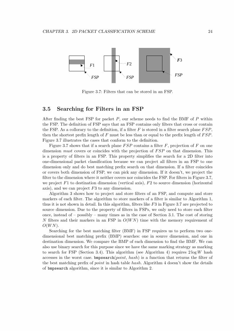
After finding the best FSP for packet P , our scheme needs to find the BMF of P withinthe FSP. The definition of FSP says that an FSP contains only filters that cross or containthe FSP. As a collorary to the definition, if a filter F is stored in a filter search plane FSP ,then the shortest prefix length of F must be less than or equal to the prefix length of FSP .Figure 3.7 illustrates the cases that conform to the definition.

Figure 3.7 shows that if a search plane FSP contains a filter F , projection of F on onedimension must covers or coincides with the projection of FSP on that dimension. Thisis a property of filters in an FSP. This property simplifies the search for a 2D filter intoone-dimensional packet classification because we can project all filters in an FSP to onedimension only and do best matching prefix search on that dimension. If a filter coincidesor covers both dimension of FSP, we can pick any dimension. If it doesn’t, we project thefilter to the dimension where it neither covers nor coincides the FSP. For filters in Figure 3.7,we project F1 to destination dimension (vertical axis), F2 to source dimension (horizontalaxis), and we can project F3 to any dimension.

Algorithm 3 shows how to project and store filters of an FSP, and compute and storemarkers of each filter. The algorithm to store markers of a filter is similar to Algorithm 1,thus it is not shown in detail. In this algorithm, filters like F3 in Figure 3.7 are projected tosource dimension. Due to the property of filters in FSPs, we only need to store each filteronce, instead of – possibly – many times as in the case of Section 3.1. The cost of storingN filters and their markers in an FSP in O(WN) time with the memory requirement ofO(WN).

Searching for the best matching filter (BMF) in FSP requires us to perform two one-dimensional best matching prefix (BMP) searches: one in source dimension, and one indestination dimension. We compare the BMP of each dimension to find the BMF. We canalso use binary search for this purpose since we have the same marking strategy as markingto search for FSP (Section 3.4). This algorithm (see Algorithm 4) requires 2 log W hashaccesses in the worst case. bmpsearch(point, hash) is a function that returns the filter ofthe best matching prefix of point in hash table hash. Algorithm 4 doesn’t show the detailsof bmpsearch algorithm, since it is similar to Algorithm 2.


Algorithm 3 Storing filters in an FSP.Require: F i = (PF isrc/LF isrc, PF idst/LF idst)Require: FSP = (PPsrc/LP, PPdst/LP )

for all F i doLenSrc ⇐ max (LF isrc, LP )LenDst ⇐ max (LF idst, LP )if LenDst > LenSrc then

HashKey ⇐ (PF idst, LF idst)insert filter F i into HashDst(FSP ) using key HashKey

elseHashKey ⇐ (PF isrc, LF isrc)insert filter F i into HashSrc(FSP ) using key HashKey

end ifend forfor all filter entries in HashDst(FSP ) do

compute and store markersend forfor all filter entries in HashSrc(FSP ) do

compute and store markersend for

Algorithm 4 Searching for the BMF of a packet.Require: P = (S,D)Require: FSP = (PPsrc/LP, PPdst/LP )

BMFsrc ⇐ bmpsearch(S, HashSrc(FSP ))BMFdst ⇐ bmpsearch(D, HashDst(FSP ))if BMFsrc is better than BMFdst then

BMF ⇐ BMFsrcelse

BMF ⇐ BMFdstend if

3.6 Storing Filters in a Search Plane

So far we have discussed about creating search planes, searching the best search plane fora packet, and searching the best matching filter for a packet in a search plane. This sectionexplains an algorithm to store filters in search planes.

Assuming that we have already created FSP of all filters, the most naive way to storefilters in FSPs is testing each filter to all FSPs to find out whether the filter has to be storedin the FSP or not. This algorithm requires N comparisons for each FSP to find all filtersthat must be stored in the FSP.

We can detect all those filter faster by the observation explained below. Suppose a filterFl = (Psrc/Lsrc, Pdst/Ldst) has to be stored in a search plane FSP (Fs) = (PPsrc/LP, PPdst/LP ),and FSP (Fl) 6= FSP (Fs). It means that FSP (Fl) must coverFSP (Fs). If we search for fil-ters in all FSPs that cover FSP (Fs), we can find all filters that must be stored in FSP (Fs).


We need to visit at most W FSPs to do this.When we visit an FSP to find filters to be stored FSP (Fs), we will have two cases like

F2 and F3 in Figure 3.7. Case of F2 is where the projection of FSP (Fs) to one dimensioncovers the filter’s projection. Case of F3 is the opposite, filter’s projection covers or matchesthe projection of FSP (Fs). To find F3, we can expand FSP (Fs) until FSP (Fs) = FSP (Fl).At each expansion of FSP (Fs), we detect whether its projection in any dimension matchesthe projection of some filters by probing HashSrc(FSP (Fl)) and HashDst(FSP (Fl)). Thisalgorithm requires at most 2W hash accesses to detect and include all filters to FSP (Fs)filter list.

For example, we have two FSPs, FSPm = (10∗, 01∗) and FSPn = (1001∗, 0110∗),and two filters F1 = (10∗, 011∗) and F2 = (10101∗, 01∗). We expand FSPn until itmatches FSPm: FSP ′

n = (100∗, 011∗), FSP ′′n = (10∗, 01∗). At FSP ′

n level, we probeHashSrc(FSPm) using 100∗ as the key. This probing returns nothing. We then probeHashDst(FSPm) using key 011∗ and it returns the hash entry for filter F1. We do thesame thing at FSP ′′

n level and probings return nothing.Figure 3.8 illustrates the expansion of FSPn. In figure (b), this process finds F1, thus

store it in the filter list of FSPn. In figure (a) and (c), this expansion doesn’t find any filters.

FSP m �

FSP �

n �

F �

1

F 2

F �

1

F 2

F �

1

F 2

(a) (b) (c)

FSP m � FSP m �

FSP �

n � ' FSP �

n � "

Figure 3.8: Expanding FSPn in FSPm to find filters.

When trying to find filters like the case of F2 in Figure 3.7, remember the marking strat-egy for filters in search plane as explained in Section 3.5. We can test whether there are filtersthat have to be stored in FSP (Fs) by probing HashSrc(FSP (Fl)) and HashDst(FSP (Fl))using the source and destination definition of FSP (Fs), respectively, to create the hash keys.If probing resulted nothing, then there is no filter that we have to store in FSP (Fs). If prob-ing matches a marker, we follow the marker down until we find the filter(s) that create(s)the marker.

The procedure above has to probe at most 2W times until it finds the hash entry for afilter. Whenever probing at prefix length l finds a marker Ml, there has to be at least onemarker or filter at prefix length l + 1. For example if a marker Ml = 1010∗ exists, there hasto be either 10101∗ or 10100∗, or both. The algorithm has to probe at both possibilitiesbecause it has no clue which one it has to probe at prefix length l+1 to get a match. Addinganother variable M.lead in marker to lead the algorithm to probe correctly will reduce thenumber of probing to W . Algorithm 5 shows this procedure.

Combining the algorithms to visit FSPs and to find filters in FSPs, we need at most2W 2 + WQ hash accesses, W : bit-width of address space, and Q: the number of filtersfound, for each FSP to find all filters that it has to store in its’ database. Algorithm 6


displays the algorithm to store all filters of an FSP into another. The cost of this algorithmis independent of the number of filters in the database, thus it is useful for large filterdatabases.

3.7 Building the Database Structure

We now have all the necessary algorithms to build the database structure of a two-dimensionalfilter database to enable a two-dimensional packet classification with search time of O(log W ).Before creating a complete algorithm to build the database, we have the following observa-tion, which reduces the time cost of the algorithm.

Previous section shows an algorithm to find all filters that have to be stored in an FSP,which costs at most 2W 2+WQ hash accesses. This is due to the assumption that an FSP hasto visit every FSPs that cover it. Suppose that we have a filter F1, which creates FSP (F1),and two search planes FSPm and FSPn; where FSP (F1) covers FSPm, and FSPm coversFSPn. If FSPn has to store F1, then FSPm also has to store F1 (see Figure 3.9).

FSP n �

FSP m �

FSP(F �

1 )

F 1

F �

2

Figure 3.9: FSPn and FSPm store F1.

This observation means that we can reduce the time to find all filters for an FSP by pro-cessing each search plane in prefix-length order, starting from the shortest up to the longestone. For example, if we have FSPm = (10∗, 11∗) and FSPn = (101∗, 110∗), we processFSPm before process FSPn. This processing order ensures that when we are processing anFSPi, the smallest search plane covering FSPi already contains all filters that FSPi has tostore, so we only have to search for the filters in one search plane. Furthermore, our markingstrategy includes variable bmsp. If we have an FSPn whose prefix length is l and we wantto find the smallest FSP, FSPm covering it, probing at l− 1 and reading its bmsp will leadus directly to FSPm. This reduces the time to store all filters in an FSP to 1 + 2W + WQ.The algorithm to build the database structure is shown in Algorithm 7.

3.8 Dealing with Wildcard Filter Problem

The design of our scheme is susceptible to wildcard filters, e.g. filters with wildcard prefixin any of their dimension. This is because of the definition of which filters can be stored inan FSP. Figure 3.10 shows the case of wildcard filters in filter database.

Figure 3.10 shows a filter database with 4 filters, where F1 is a wildcard filter whosedestination dimension is the one with wildcard prefix. Let’s consider the filter database if


F1 doesn’t exist. If F1 doesn’t exist, then each FSP in this example only stores the filtercreating it. If F1 exists, then FSP (F2), FSP (F3), and FSP (F4) has to store F1. Thissituation is like F2 and F3 of Figure 3.7, but in a much larger scale.

src

dst

F 2

F �

3

F �

4 �

F �

1

FSP ( F 3)

FSP �

( F �

4) �

FSP �

( F �

2)

Figure 3.10: A wildcard filter in filter database.

One way to remove the effect of wildcard filters is not to store them in any FSPs exceptin its search plane. With this strategy, we have an additional step to find the correct bestmatching filter. The additional step is if the best FSP has non-zero prefix length and wefail to find the BMF in that FSP, we have to do another search for BMF in the zero prefix-length FSP. Thus, we have to do 5 log W hash accesses in the worst case. This strategy isa time–space trade-off.

This strategy completes the design of a two-dimensional packet classification of thisthesis. Next chapter will discuss the simulations for this scheme.


Algorithm 5 Follow markers to find filters.Require: Prefix to follow; HashTable storing markers

HashKey ⇐ PrefixMarkSrc ⇐ probe HashTable using HashKeyif MarkSrc exists then

i ⇐ 0PrefChild ⇐ NULLloop

LABEL Loop0:Follow[i].marker ⇐ MarkSrcFollow[i].visit0 ⇐ 0 ; Follow[i].visit1 ⇐ 0if MarkSrc is a filter then

add MarkSrc to FilList arrayend ifif MarkSrc.lead leads to child 0 then

Follow[i].visit0 ⇐ 1end ifif MarkSrc.lead leads to child 1 then

Follow[i].visit1 ⇐ 1end ifLABEL Loop1:if Follow[i].visit0 = 1 then

Follow[i].visit0 ⇐ 0PrefChild ⇐ PrefChild · 0HasKey ⇐ Prefix · PrefChildMarkSrc ⇐ probe HashTable using HashKeyif MarkSrc exists then

i ⇐ i + 1 ; goto Loop0end if

end ifif Follow[i].visit1 = 1 then

Follow[i].visit1 ⇐ 0PrefChild ⇐ PrefChild · 1HashKey ⇐ Prefix · PrefChildMarkSrc ⇐ probe HashTable using HashKeyif MarkSrc exists then

i ⇐ i + 1 ; goto Loop0end if

end ifi ⇐ i− 1if i < 0 then finishPrefChild ⇐ PrefChild⊗ i ; goto Loop1

end loopend if


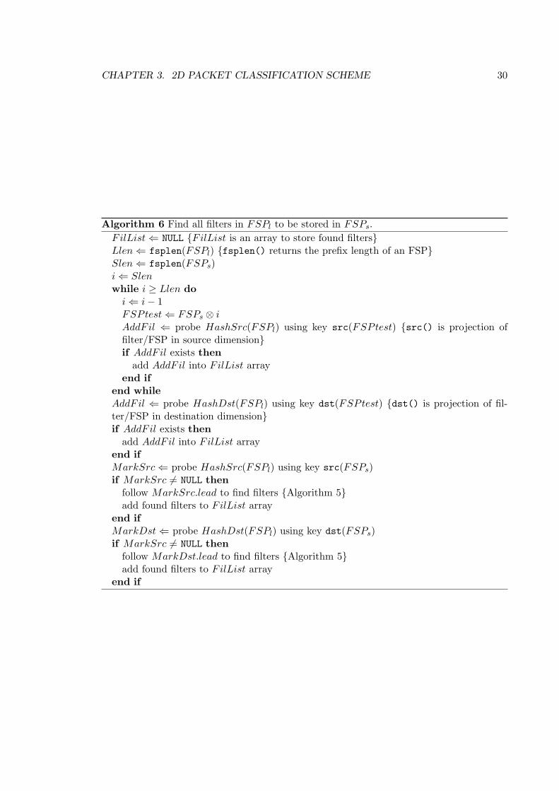
Algorithm 6 Find all filters in FSPl to be stored in FSPs.FilList ⇐ NULL {FilList is an array to store found filters}Llen ⇐ fsplen(FSPl) {fsplen() returns the prefix length of an FSP}Slen ⇐ fsplen(FSPs)i ⇐ Slenwhile i ≥ Llen do

i ⇐ i− 1FSPtest ⇐ FSPs ⊗ iAddFil ⇐ probe HashSrc(FSPl) using key src(FSPtest) {src() is projection offilter/FSP in source dimension}if AddFil exists then

add AddFil into FilList arrayend if

end whileAddFil ⇐ probe HashDst(FSPl) using key dst(FSPtest) {dst() is projection of fil-ter/FSP in destination dimension}if AddFil exists then

add AddFil into FilList arrayend ifMarkSrc ⇐ probe HashSrc(FSPl) using key src(FSPs)if MarkSrc 6= NULL then

follow MarkSrc.lead to find filters {Algorithm 5}add found filters to FilList array

end ifMarkDst ⇐ probe HashDst(FSPl) using key dst(FSPs)if MarkSrc 6= NULL then

follow MarkDst.lead to find filters {Algorithm 5}add found filters to FilList array

end if


Algorithm 7 Build database structure for a filter database.Require: N filters, F i, 0 ≤ i < N

for all filter Fi 0 ≤ i < N doif FSP (F i) not exists then

create search plane FSP (F i)store FSP (F i) based on prefix length order, short to long

end ifstore F i in FSP (F i) {Algorithm 3}

end forfor all FSPk in sorted FSP list, 0 ≤ k < M do

FSPup ⇐ NULLLen ⇐ fsplen(FSPk) {fsplen() returns the prefix length of an FSP}Len ⇐ Len− 1HashKey ⇐ FSPk⊗ LenFSPup ⇐ probe HashTable(Len) using HashKeyHashKey ⇐ FSPk⊗ FSPup.bmspFSPup ⇐ probe HashTable(FSPup.bmsp) using HashKeyif FSPup 6= NULL then

FilList ⇐ get all filters to be stored in FSPk {Algorithm 6}store filters of FilList in FSPk {Algorithm 3}

end ifend for

Chapter 4

Simulation

This chapter presents the details of data structure in implementing 2D packet classificationscheme of Chapter 3. This chapter doesn’t give any details of the pseudo-codes of theimplementation because they are based on the algorithms explained before. This chapterthen explains filter database design for our simulation and presents the simulation results.

4.1 The Implementation Data Structure

The algorithms of our scheme are implemented in C language for simulation purpose. Thissection explains details of the data structure used for our packet classification scheme.

When we read a filter database, we store it as an array of filters. Using an array of filterseases random access to each filter by only using filter’s index value. Each filter is storedas two tuples of prefix and prefix length pair and a number to represent its index value.Figure 4.1 shows the data structure for a filter.

Besides storing it in an array, we also have to store it, probably several times, in a hashtable as a marker for filter. The data structure for a filter marker is shown in Figure 4.2.This data structure has lead element to be used by Algorithm 5 to store other filters in anFSP, and bmp to store best matching prefix. This marker also stores pointer to a filter. Thiselement points to the memory location of a filter if it is really a marker to a filter, otherwiseit contains NULL.

We store an FSP twice: in a linked list and in a hash table. Figure 4.3 shows the datastructure used to represent an FSP. This structure stores FSP definition similar to the data

typedef struct filter_ {u_int32_t src_prefix;u_int src_preflen;u_int32_t dst_prefix;u_int dst_preflen;u_int32_t fil_num;

} filter;

Figure 4.1: Data structure for a filter.

32

CHAPTER 4. SIMULATION 33

typedef struct fil_mark_ {u_int lead, bmp;filter *filter;

} fil_mark;

Figure 4.2: Marker for a filter.

typedef struct fsp_data_ {u_int32_t src_prefix;u_int src_preflen;u_int32_t dst_prefix;u_int dst_preflen;fsp_mark *marker;

} fsp_data;

Figure 4.3: An FSP.

typedef struct fsp_mark_ {u_int bmsp, flsize;filter **flist;

} fsp_mark;

Figure 4.4: Marker for an FSP.

structure of a filter, since as stated in the previous chapter, an FSP is also can be viewedas a filter. This structure also stores pointer to a marker in a hash table representing thisFSP.

A marker for FSP has the bmsp element, the best matching search plane, which is usedduring searching for the best FSP. A marker that represents an FSP, contains at least 1filter. flsize and flist form the filter list of an FSP. Element flsize indicates how many filtersare contained within the FSP. If flsize is not 0, then this marker represents an FSP and thecontained filters can be found by looking in flist. flist is a pointer to an array of pointers tofilter. We use this strategy to reduce memory usage because a filter can be stored in morethan one FSP, thus it is better for an FSP to store pointers to filter instead of the filters.This data structure is shown in Figure 4.4.

The basic data structure for this scheme is hash table. The scheme implies that we needto have (W + 1) + 2N hash tables: W + 1 hash tables for storing FSP entries, and 2 hashtables to store filter’s projections in an FSP for each of N FSPs of the filter database.However, for the ease of implementation, we only use three hash tables: one for FSPsand one for each filter projection in source and destination dimension. This is possible byincluding prefix length in the hash key of each entry and including FSP definition in caseof filter entry. With this strategy, hash key for an FSP entry and a filter are a two tuplesand three tuples, respectively, of prefix and prefix length pair. For example, we have a filter(10/8, 192.168/24). The FSP for this filter is (10/8, 192/8). Hash keys for its FSP and filter


typedef struct fsp_key_ {u_int32_t src_prefix;u_int src_preflen;u_int32_t dst_prefix;u_int dst_preflen;

} fsp_key;

Figure 4.5: Data structure of FSP hash key.

typedef struct fil_key_ {u_int32_t src_prefix;u_int src_preflen;u_int32_t dst_prefix;u_int dst_preflen;u_int32_t fil_prefix;u_int fil_preflen;

} fil_key;

Figure 4.6: Data structure of filter hash key.

entries are (10/8, 192/8) and (10/8, 192/8, 192.168/24). Figure 4.5 and Figure 4.6 show thedata structure of each hash key.

4.2 Simulation Filter Database Design

We use simulation to evaluate the performance of our 2D packet classification scheme.Using simulation, we want to know the time to build data structure for filter databasesand memory usage of our scheme. The worst-case search time of this scheme is O(log W ),which is considerably fast. Memory usage, however, should receive more attention since ourscheme tries to reduce the probability to reach the worst case of O(N2). In this simulation,we want to know how our scheme will perform in real-life filter databases.

To simulate this scheme, we create random and non-random two-dimensional filterdatabases based on the publicly available Internet routing table. Randomly creating fil-ter databases approach is also used by [3], [7], and [10]. However, [3] and [7] do not giveany detail on how to create filter databases. Creating random filter databases straight fromInternet routing table would not result in filters that we can use to evaluate our scheme.Therefore we want artificial filter databases for our simulation can be used as a baseline tomeasure the performance of our scheme, especially for the memory requirement.

[10] attempts to model large filter databases and creates random filter databases basedon that model. The basic idea is to classify network elements into distinct types, e.g. work-station hosts, server hosts, subnet border routers, enterprise core routers, enterprise edgerouters, ISP edge routers, ISP core routers, and ISP peering routers. For each class, theapplications and their filter tables are identified. Based this model, [10] projects that ISPedge routers class has to support the largest number of filters and enterprise edge routers


class is next.For our simulation we choose to use Autonomous System (AS) as the base to create

filters and routers having these filters are AS border routers. We choose to use AutonomousSystems because even though an AS is defined as a group of IP networks operated by oneor more network operators which has a single and clearly defined external routing policy,in practice an AS usually belongs to a single ISP or enterprise. Because of this, it is likelythat an Autonomous System also has a single security (firewall) and QoS policy.

AS-A AS-A BR

AS-B

AS-B BR

AS-C AS-C BR

Figure 4.7: AS border routers.

We choose to simulate filter databases running on AS border routers, and we createfilter databases from prefixes of two ASes. An AS border router connects an AutonomousSystem to another (Figure 4.7). It is the entrance and exit points for packets originatedfrom and destined to the corresponding AS. It is usually where filter database is the mostcomplete compared to the other filter databases in that AS. If we use the model by [10], anAS border router can be categorized as an ISP edge router or as an enterprise edge router,depending on whether the particular AS is owned by an ISP or an enterprise.

In selecting ASes for this simulation, we use the Internet routing table made available byTelstra Network, Australia [1]. This routing table consists of around 100 thousand prefixesand about 12 thousand ASes advertise those prefixes. First we separate prefixes by theiroriginating AS number and we view prefixes of an AS as a single routing table. We processeach routing table by counting the number of prefixes, maximum prefix level, duplicatedprefixes and the ratio of duplicated prefixes to the number of prefixes.

Prefix level is a measure that counts the number of prefixes of a given IP address ina routing table. For example, we have a routing table consists of four entries: 10.1.1/24,10.1/19, 10.1/16, and 10.1.224/23. For IP address 10.1.1.1 we have three prefixes, and forIP address 10.1.224.2 we have two prefixes. The maximum prefix level of our routing tableis 3.

Duplicated prefixes shows the number of times prefixes are stored in other prefixesbecause the former cover the latter. For example, suppose we have an AS consists of 4prefixes: A, B, C, and D. A is a prefix of B, B is a prefix of C, and none of A, B, C isa prefix of D. This AS has maximum prefix level of 2 (A and B are prefixes of C) andduplicated prefixes of 3 (A is stored in B and C, and B is stored in C).


Table 4.1: ASes for cross-product filter databases.

AS num Prefixes Level Dup. pref. % Dup. pref.680 230 1 0 0.00%786 183 1 0 0.00%1913 124 1 0 0.00%4713 117 1 0 0.00%517 111 1 0 0.00%4151 366 4 589 160.93%2907 366 2 2 0.55%2007 166 2 110 66.27%719 166 2 32 19.28%

11492 111 4 194 174.77%7657 111 2 18 16.22%

4.2.1 Cross-producting prefixes

Our scheme could reach O(N2) if there are duplicated prefixes in filter database (Figure 3.5).Looking at our scheme and the result of processing BGP routing table, our hypothesis isan AS whose duplicated prefixes percentage is high has high probability to result in highnumber of filters in structure compared to the number of filters in filter database.

For this simulation, We use filter databases created by cross-producting prefixes of twoASes: one that has duplicated prefixes, and one with no duplicated prefixes. We simulatethese filter databases to confirm our hypothesis. For ASes without duplicated prefixes, weselect five ASes whose number of prefixes rank on the top. For ASes with duplicated prefixes,we select three sets of ASes whose number of prefixes are equal. These ASes are displayedin Table 4.1.

4.2.2 Random prefixes

For filter databases consisted of random prefixes, we rank the ASes based on the four valuesabove. Tables 4.2 to 4.5 show the top 5 ASes of each category. From these tables we have16 distinct ASes, because several ASes appear twice.

Table 4.2: AS ranked by number of prefixes.

AS num Prefixes Level Dup. pref. % Dup. pref.701 2202 3 426 19.35%1221 1422 3 176 12.38%7018 1091 2 156 14.30%702 1053 3 170 16.14%1 844 3 175 20.73%


Table 4.3: AS ranked by maximum prefix level.


Table 4.4: AS ranked by duplicated prefixes.


Table 4.5: AS ranked by percentage of duplicated prefixes.


We create two types of random filter databases for our simulations:

1. database with only non-wildcard filters

2. database with wildcard and non-wildcard filters

To create a non-wildcard filter database for this simulation, we select two ASes out of the16 distinct ASes, namely AS-A and AS-B, create random prefixes from the prefixes of eachAS, and we join two prefixes, one from AS-A and one from AS-B to form a two-dimensionalfilter.

A random prefix of an AS is formed as follows:

1. select Prefix randomly from prefixes of AS

2. select Subplen randomly between 0 and 32−prefix length of Prefix

3. create SubPrefix as a random binary string with length of Subplen


4. concatenate Prefix and SubPrefix to create the result.

Simulating the non-wildcard filter databases, we make the combinations of all distinctASes, thus we have 120 combinations. For each combination we create filter databasesconsisting of 2000, 4000, 10000, 20000, 40000, and 80000 filters, where for each size wecreate 5 filter databases.

For the case of filter databases with wildcard filters, we want to know the memoryrequirement of our scheme without the solution that is explained in Section 3.8. We choose6 of above filter databases, formed by the pair of AS 701, 4787, 8010, and 9796 that consistsof 20000 filters. We create wildcard filters sized 50, 100, 200, 500, 1000, and 2000 filters,containing random prefixes based on the prefixes of each AS. We add a wildcard filterdatabase to the non-wildcard filter database formed from the same AS, thus we have 72filter databases. For example, we add a wildcard filter created from AS 701 to non-wildcardfilters created from AS 701 and 8010 pair.

We compile and run our implementation for each filter database on a Pentium III 1GHzmachine running FreeBSD 4.3-RELEASE. This implementation is compiled using gcc with-out any compile time optimizations.

We record the memory requirement of each filter database and the time to build thedata structure for non-wildcard filters. The build time is measured as user time in secondsobtained from getrusage() system call. Memory requirement is measured as the numberof filters stored in all filter search planes. Results of these simulations are shown in the nextsections. For filters with non-wildcard filters we average the data obtained from 5 filterswhose AS pair and sizes are same before we present the results.

We also run the basic 2D packet classification scheme that is explained in Section 3.1using several filter databases for comparison with our scheme.

4.3 Cross-product Filter Database Result

We display the result of our scheme for cross-product filter databases. Table 4.6 shows thenumber of filters stored in our scheme and Table 4.7 shows the numbers relative to filterdatabase size.

Table 4.6: Filters in structure of cross-product filters.

AS 680 786 1913 4713 5174151 93708 72097 45474 48693 463782907 84280 67024 45384 42916 407142007 41325 31639 20584 21225 20541719 39809 31295 20599 20721 19615

11492 26944 20888 13764 13869 133217657 25792 20417 13764 13139 12501


Table 4.7: Percentage of filters in structure of cross-product filters.

AS 680 786 1913 4713 5174151 111.319% 107.643% 100.198% 113.710% 114.158%2907 100.119% 100.069% 100.000% 100.220% 100.217%2007 108.237% 104.151% 100.000% 109.283% 111.478%719 104.267% 103.019% 100.073% 106.688% 106.453%

11492 105.539% 102.831% 100.000% 106.791% 108.116%7657 101.026% 100.512% 100.000% 101.170% 101.461%

4.4 Random Non-wildcard Filter Database Result

4.4.1 Build time

Figure 4.8 shows the time required to build data structure for the filter database. x andy axes are the number of filters in database (in thousands) and time to build the datastructure (in seconds).

1.572

22.817

7.216

16.280

3.419

8.454

1.574 3.296

0 �

5 �

10

15

20

25

0 �

10 20 �

30 �

40 �

50 �

60 �

70 80 �

90 �

filter database size (N) �

build

tim

e (s

ec)

Figure 4.8: Time to build the data structure for all filter database.

4.4.2 Memory requirement

This sub section shows the memory requirement results for our simulations. The memoryrequirement is shown as the average number of filters stored in all FSPs of 5 random filterdatabases with same AS pairs and size. Figure 4.9 shows the combined result for all AS pairsand sizes. The x axes is the number of filters in filter database and y axes is the number offilters in the data structure of our scheme. Both x and y axes are shown in thousands scale.

To get more insight on the memory requirement, this sub section shows several figures ofthe number of filters in structure, which is shown as the relative percentage of the number


2.000 4.000 10.003

20.009

40.044

80.163

36.654

78.507

163.415

5.538

16.366

0 �

20

40

60 �

80 �

100

120

140

160

180

0 �

10 20 30 �

40 50 �

60 �

70 80 �

90 �

filter database size �

filte

rs in

str

uctu

re

Figure 4.9: Filters in structure for all combinations.

of filters in the database. We show the result of filter databases created by pairing one ofthese ASes with the others: AS 701, 4787, 8010, and 9796. These AS rank number one ineach category. We also display the result of AS 9796 because AS 4787 ranks number onetwice and AS 9796 ranks second in both categories.

100.46 101.01 102.38

104.62

108.89

116.25

90.00 �

95.00 �

100.00

105.00

110.00

115.00

120.00

0 �

10 20 30 �

40 50 �

60 �

70 80 �

90 �


filte

r in

str

uctu

re (

%of

N)

1221 7018 702 1 4787 4323 6172 �

7843

Figure 4.10: Filters of AS 701 pairing with other top 5 of prefix and level ASes.


100.62 101.18 102.44

105.03

109.21

116.65

90.00 �

95.00 �

100.00

105.00

110.00

115.00

120.00

0 �

10 20 �

30 �

40 �

50 �

60 �

70 80 �

90 �


filte

r in

str

uctu

re (

%of

N)

8010 �

4151 3967 �

9796 �

12150 21529 7908

Figure 4.11: Filters of AS 701 pairing with other top 5 of duplicated prefix and the percent-age ASes.

107.14

114.90

126.55

139.05

153.57

170.47

90.00 �

100.00

110.00

120.00

130.00

140.00

150.00

160.00

170.00

180.00

0 �

10 20 30 �

40 50 �

60 �

70 80 �

90 �


filte

r in

str

uctu

re (

%of

N)

701 1221 7018 702 1 4323 6172 �

7843


134.99

149.80

172.46

186.47

194.91 199.83

90.00 �

110.00

130.00

150.00

170.00

190.00

210.00 �

0 �

10 20 30 �

40 50 �

60 �

70 80 �

90 �


filte

r in

str

uctu

re (

%of

N)

8010 �

4151 3967 �

9796 �

12150 21529 7908

Figure 4.13: Filters of AS 4787 pairing with other top 5 of duplicated prefix and the per-centage ASes.


103.15 105.18

110.83

118.42

128.08

139.42

90.00 �

100.00

110.00

120.00

130.00

140.00

150.00

0 �

10 20 30 �

40 50 �

60 �

70 80 �

90 �


filte

r in

str

uctu

re (

%of

N)

701 1221 7018 702 1 4787 4323 6172 �

7843


102.26 104.11

110.00

116.39

126.65

139.23

90.00 �

100.00

110.00

120.00

130.00

140.00

150.00

0 �

10 20 �

30 �

40 �

50 �

60 �

70 80 �

90 �


filte

r in

str

uctu

re (

%of

N)

4151 3967 �

9796 �

12150 21529 7908


134.99

149.80

172.46

186.47

194.91 199.83

90.00 �

110.00

130.00

150.00

170.00

190.00

210.00

0 �

10 20 30 �

40 50 �

60 �

70 80 �

90 �


filte

r in

str

uctu

re (

%of

N)

701 1221 7018 702 1 4787 4323 6172 �

7843



139.69

152.44

172.52

182.61

194.58 198.15

90.00 �

110.00

130.00

150.00

170.00

190.00

210.00

0 �

10 20 30 �

40 50 �

60 �

70 80 �

90 �


filte

r in

str

uctu

re (

%of

N)

8010 �

4151 3967 �

12150 21529 7908


4.5 Random Wildcard Filter Database Result

Figures 4.18 to 4.21 display the effect of adding wildcard filters to non-wildcard filterdatabase. Each figure shows the result when we add wildcard filters created from an AS toa filter database sized 20000 filters. x axes is the number of wildcard filters and y axes isthe number of filters in the structure relative to filter database size.

105.22 106.20

107.52

110.46

115.90

123.88

100.00

105.00

110.00

115.00

120.00

125.00

130.00

0 �

500 �

1000 1500 2000 2500

wildcard filters �

filte

rs in

FS

P (

% o

f N)

4787 8010 �

9796 �

Figure 4.18: Adding wildcard filters created from AS 701.


165.34

203.94

246.62 267.87

412.21

488.56

100.00

150.00

200.00

250.00 �

300.00 �

350.00 �

400.00 �

450.00 �

500.00 �

0 �

500 �

1000 1500 2000 2500


filte

rs in

FS

P (

% o

f N)

701 8010 �

9796 �


105.04 108.08

112.19

127.11

147.49

172.53

100.00

110.00

120.00

130.00

140.00

150.00

160.00

170.00

180.00

0 �

500 �

1000 1500 2000 2500


filte

rs in

FS

P (

% o

f N)

701 4787 9796 �


286.02

313.17

408.80

472.61

161.15

165.43

100.00

150.00

200.00

250.00 �

300.00 �

350.00 �

400.00 �

450.00 �

500.00 �

0 �

500 �

1000 1500 2000 2500


filte

rs in

FS

P (

% o

f N)

701 4787 8010 �



4.6 Memory Requirement of the Scheme in Section 3.1

We show in Figure 4.22 the result of simulations using the scheme in Section 3.1 for threefilter databases, formed by pairing prefixes from AS 701 with the ones from AS 4787, 8010,and 9796. We do not perform many simulations using this scheme since the purpose is onlyas a comparison with our scheme.

664.15 1160.30

2481.26

3857.08

5535.34

8055.06

944.25

0 �

2000 �

4000 �

6000 �

8000 �

10000

0 �

10 20 30 �

40 50 �

60 �

70 80 �

90 �


filte

rs in

str

uctu

re (

% o

f N)

4787 �

8010 �

9796 �

Figure 4.22: Filters of AS701 using the scheme in Section 3.1.

Chapter 5

Analysis and Evaluation

This chapter analyzes and evaluates our 2D packet classification scheme based on schemes’design and the simulation results. First we analyze the effect of duplicated prefixes tomemory requirement, then we look into memory requirement of randomly generated filterdatabase. We also analyze the time to build our data structure. We close this chapter bygiving general evaluation of our two-dimensional packet classification scheme.

5.1 Effect of Duplicated Prefixes

Our hypothesis regarding this scheme is higher percentage of duplicated prefixes of filters indatabase can cause higher number of filters in the structure. Numbers in Table 4.7 seem toconfirm this hypothesis, in general. We can see that filter databases created by ASes whosenumber of prefixes are the same but higher percentage of duplicated prefixes have higherpercentage of filters in structure, except for the ones paired with AS 1913. When our filterswith duplicated prefixes are paired with AS 1913, there is no consistent pattern that showsthe effect of duplicated prefixes. AS 4151 has higher numbers than AS 2907, AS 2007 haslower numbers than AS 719, and AS 11492 and AS 7657 has the same numbers.

For our cross-product filter database case, a filter could be stored in more than one FSPonly if the next conditions hold. Let’s consider that we have a filter database created fromAS A and B. AS A has no duplicated prefixes, while B has some, and there is a prefix PB1covering PB2 in B and a prefix PA1 in A. PB1 could be stored in more than one FSPonly if the prefix length of PB1 is shorter than that of PA1 and the prefix length of PB2is longer than that of PA1. Figure 5.1 pictures this case. F11, formed by PA1 and PB1, isstored in two FSPs, FSP (F11) and FSP (F12).

A probe into prefixes of AS 1913 shows that all but five prefixes have prefix length of24, and all those five prefixes have the length of 16. Looking into all ASes paired with AS1913, we found that:

1. there is no prefix having length larger than 24,

2. only AS 4151 and 719 have prefixes whose length is less than 16 covering other prefixes.

These observations explain why we found low number of filters in structure for the crossproducts of AS 1913 with other ASes in our simulation. These also explain why AS 719

46

CHAPTER 5. ANALYSIS AND EVALUATION 47

PA �

1

PA 2

PB2

PB 1

F 21

F �

11 F �

12

F 22

Figure 5.1: F11 is stored in FSP (F11) and FSP (F12).

has higher number of filters than AS 2007 even though AS 2007 has higher percentage ofduplicated prefixes.

Analysis on this section shows that our hypothesis doesn’t always hold. The reason forthis is if we have two filters F1 and F2 where F1 covers F2 in one dimension, then whetherF1 has to be stored in FSP (F2) depends on the value of the other dimension of both filters(see Figure 3.5). However, this hypothesis can be used as a baseline to qualitatively predictthe number of filters in structure of a filter database.

5.2 Memory Requirement

5.2.1 Non-wildcard filter database

Our results for non-wildcard filter databases show that, in general:

1. filter databases that we used in our simulations require at most about twice of thenumber of filters in the database (see Figure 4.9).

2. filter databases formed by ASes whose number of prefixes is small have higher per-centage of filters in structure.

3. while the percentage of filters in structure increases as the number of filters in databaseincrease, the trend shows that the increase in percentage is getting smaller.

Looking at Figures 4.10 to 4.17 and sorting them by the number of prefixes, we have thedescending order of AS 701, 8010, 4787, and 9796. The series in each figure whose valuesare displayed are the ones that have the highest filters in structure when filter databasesize is 80-thousand filters. These series are shown in Figure 5.2. From this figure we cansee that the order of these series from the lowest percentage to the highest one follows thedescending order of ASes’ number of prefixes.


90.00 �

110.00

130.00

150.00

170.00

190.00

210.00

0 �

10 20 30 �

40 50 �

60 �

70 80 �

90 �

filter database size �

filte

rs in

str

uctu

re

701 (4787) 701 (12150) 8010 (4787) �

8010 (12150) �

4787 (7843) 4787 (9796) 9796 (4787)

�9796 (12150) �

Figure 5.2: Top series of top 4 ASes.

The main reason for this is because at the same number of filters in our simulation,an AS whose number of prefixes is smaller generates more filters per ASes’ prefix than theone with more prefixes. If we extract the field of filters generated from prefixes of a certainAS, we can see that more filters per prefix increases the probability of duplicated prefixes.Table 5.1 shows the distinct and duplicated prefixes generated from these four ASes. Fromthese tables we can see that duplicated prefixes increase as the filter size increases, and ASeswhose number of prefixes is small has higher probability to get more duplicated prefixes (inpercentage) at the same filter database size.

Higher percentage of duplicated prefixes in our simulation means that the probabilityof having filters stored more than once increases. This is what we see in our memory re-quirement results. In our simulation, we generate prefixes of both dimensions of our filterdatabases randomly, thus it is difficult to predict how much filters have to be stored in morethan one FSP.

Another trend that we see from Table 5.1 is the increase rate of distinct prefixes of an ASdiminishes as the size of filter database increases. This trend exists because the more distinctprefixes created by random generator, the probability that the newly created prefixes willhave the same value as the existing ones increases, therefore reducing the increase rate ofdistinct prefixes. This trend is also shown in our simulation result.

The above analysis shows that:

1. the increase of duplicated prefixes in the filter database contributes to the percentageincrease of filters in structure

2. the diminishing increase rate of filters in structure as filter size increases is contributedby the increase rate of distinct prefixes, which is created randomly, is slowing.

5.2.2 Adding wildcard filters

Looking at the effect of wildcard filters if we run our scheme without the strategy of Sec-tion 3.1, we can see that adding wildcard filters created from AS 701 adds the percentage of


Table 5.1: Distinct and duplicated prefixes of ASes in filter databases.

AS 701 AS 8010db size prefixes dupl. pct. dup. prefixes dupl. pct. dup.

2k 993 84 8.46% 988 528 53.44%4k 1971 339 17.20% 1915 1430 74.67%10k 4825 1805 37.41% 4515 8994 199.20%20k 9396 7661 81.53% 8349 26887 322.04%40k 17950 24356 135.69% 14911 70876 475.33%80k 33195 74070 223.14% 25343 160992 635.25%

AS 4787 AS 9796db size prefixes dupl. pct. dup. prefixes dupl. pct. dup.

2k 777 5531 711.84% 791 4792 605.82%4k 1358 10280 757.00% 1432 9980 696.93%10k 2786 25969 932.12% 2846 24472 859.87%20k 4456 45497 1021.03% 4752 44830 943.39%40k 6965 75504 1084.05% 7406 75010 1012.83%80k 9854 111754 1134.10% 10809 115216 1065.93%

filters in structure of all filter databases of our simulation at roughly the same rate. On theother hand, the other three cases of wildcard filters additions don’t show significant increasein percentage except for filter databases pairing with AS 701. Some filter databases evenshow a decrease in number of filters’ percentage.

A pattern that we see here the ASes’ number of distinct prefixes contributes to thedifference percentage increase. This pattern is already discussed in the previous section,i.e. there are more filters per prefixes of an AS with lower number of distinct prefixes at acertain filter database size.

Another pattern is when wildcard filters are created from AS 4787, 8010, or 9796, filterdatabases created from AS 701 show a very high increase in number of filters’ percentage.The other filter databases don’t display this result. The main reason for this is AS 701 hashigher number of top-level prefixes both in absolute and relative figures. A top-level prefixof a routing table is a prefix that is not covered by another prefix. Table 5.2 shows thenumber of distinct and top level prefixes of an AS.


Table 5.2: Distinct and top level prefixes of AS

AS num Prefixes Top level701 2202 18134787 47 18010 720 229796 38 2

5.3 Build Time

Complexity analysis on the algorithms of our scheme shows that the time to build thedata structure in memory is linear with the number of filters in filter database. CreatingFSPs and their markers takes O(NW ), storing filters in FSPs requires O(NW + WQ), andmarking filters needs O(NW ) time. If no filter is stored more than once, then Q = 0, thusthe build time is simply O(NW ). Because W , the bit-width of address, is a constant, thenthe build time is linear with N .

The fastest time to build data structure at each filter database size in Figure 4.8 is thecase where build time is O(NW ) because the lowest figures in Figure 4.9 shows the numberof filters in data structure is almost equal to the number of filters in the database. Thelowest build times show that they are not linear to the number of filters. This is most likelydue to cache memory misses. The more filters in database, the more memory and timeare required. Using more memory means that less portion of the data structure fits in theprocessors’ cache memory and it forces the processor to get the data from main memorymore frequently. More time to build the data structure means that the operating system wasprobably doing more context-switching during the process. This also affects cache memoryusage. This explains the deviation of build time from linear time, in case of no filter is storedmore than once.

5.4 General Evaluation

In general our scheme is able to reduce memory usage compared to the basic scheme ofSection 3.1. We can see from Figure 4.22 that the basic scheme requires very large memorybecause the probability of reaching O(N2) memory is high. Simulations of our scheme onthe same filter databases show that our scheme saves much memory compared to the basicscheme even though both schemes have same worst-case memory requirement. This memoryreduction comes with additional cost in time to search for the best matching filter, thus wecan view our scheme as a time–space tradeoff of the basic scheme.

We evaluate the performance of this 2D packet classification scheme using simulatedfilter databases. While these filter databases are not the real ones, we believe that ourmethod in generating them is sufficient to simulate real-life filter databases.

We do not simulate the search time of our scheme because complexity analysis of searchtime already shows that it is considerably fast and it is independent from the number offilters in database. Time to build data structure of our scheme is linear to the number of


filters, however we also need additional time in this process, which is linear to the numberof duplicated filters. This linear build time is reached through several observations of therelationship between filters and FSPs.

A limitation of our 2D packet classification scheme is we cannot extend the schemeinto more than two dimensions without reducing its memory saving capability. On a two-dimensional filter database, a filter marker in our scheme stores only one filter, which is thebest one. This is not the case for higher dimensional filters. If we use this scheme for higherdimension filter database, whenever filters conflict in the source and destination fields, ourscheme has to store all of them in order for the search algorithm to return the correct bestmatching filter. Therefore, the benefit of our scheme is reduced.

Chapter 6

Conclusion

6.1 Summary

In this thesis we described packet classification problem. Then we proposed a scheme forclassifying Internet packet based on source and destination address fields to solve this prob-lem. To evaluate our scheme, we performed simulation using randomly generated filterdatabases and we presented the results.

We explained packet processing in Internet routers and showed that an Internet routercould process a packet several times using a function, which is packet classification, for dif-ferent applications: QoS, firewall, etc. We showed that Internet routers need to have a goodpacket classification function so they can forward Internet packets as fast as their interfaceline speeds. This thesis then described the packet classification formally and summarizedseveral related works in this fields.

The objective of a packet classification is to find the best matching filter (BMF) ofa packet. This thesis explained a two-dimensional packet classification scheme, where thebasic idea is to create many search planes and store filters in search planes. To search forthe BMF of a packet, we use a two-step process:

1. search for the search plane containing BMF,

2. and then search for BMF in that search plane.

We create a search plane based on filters’ definition. The assumption that we used inthis research is fields of a filter can only take the form of prefixes. With this assumptionwe can create a search plane for a filter by using the shortest prefix length of the filter.We store a filter in a search plane if the filter crosses or covers the search plane. Using thisstrategy, a filter could be stored in more than one search plane, depending on the definitionof both the filter and the search planes.

This scheme has the worst-case search time of O(log W ). Through several observations,we are able achieve O(NW + QW ) time to build our data structure. N is the number offilters in filter database; W is the bitwidth of IP address; and Q is the number of duplicatedfilters. The worst-case memory requirement of our scheme is O(N2W ), however our schemeis designed to reduce the probability of reaching that worst-case. We also observed thatwe can prevent memory explosion caused by wildcard filters by separating them from non-wildcard filters. This can be achieved with an extra cost in search time.

52

CHAPTER 6. CONCLUSION 53

This thesis evaluated the performance of our scheme using randomly generated filterdatabases. We modeled filter databases running on Autonomous System boundary routers.We ran our scheme using various random filter databases with different size. The simulationresults showed that the memory usage tends to be closer to O(NW ) even though the worst-case is O(N2W ). This is an important result of our scheme, which has never been exploredbefore by others.

Table 6.1 shows our scheme among the other two-dimensional packet classificationschemes. We can see that the worst-case lookup time and memory usage are comparable tocross-producting scheme. However, cross-producting tends to come close to the worst-casememory usage, and to reduce the memory usage, it uses a method to build data structureon-demand.

Table 6.1: Our scheme and other 2D packet classification schemes.

Scheme Lookup time Memory usageTuple space search O(W 2) O(N)Rectangle search O(W ) O(NW )Pruned tuple space O(W 2) O(N)Grid of tries O(W ) O(NW )Cross-producting O(log W ) O(N2)Fast-2D O(log2W ) O(N log2W )Our Scheme O(log W ) O(N2W )

6.2 Future Work

A limitation of our scheme is we can use it for higher dimension packet classification,but with a reduction in memory saving capability. The main reason for this is for two-dimensional classification case, our scheme only needs to store the best filter in case ofconflicting filters, but we cannot do this in higher-dimension case. This thesis does notaddress this problem. In the future, we will explore the performance of our scheme forhigher-dimension packet classification.

Acknowledgments

I would like to thank Professor Jun Murai, Associate Professor Hiroyuki Kusumoto, andProfessor Suguru Yamaguchi of Nara Advanced Institute of Science and Technology forall their help and advise even before the start of my study in Japan. I would also thankAssociate Professor Osamu Nakamura, Assistant Professor Masaki Minami, and other mem-bers of Murai Lab. Special thank goes to members of AI3 (Asian Internet InterconnectivityInitiatives) and INSAT group: Hidetaka Izumiyama, Mikiyo Nishida, Haruhito Watanabe,Shoko Mikawa, Shunsuke Fujieda, Ayumu Yasuda, and the bachelor degree students.

A very special thank goes to my wife – Endrieta Virnakhristi –, my child – ShafiyyaNurul Izza –, and my other family members for their love and support. Thank you.

54

Bibliography

[1] http://www.telstra.net/ops/bgp/index.html.

[2] F. Baker, 1995. Requirements for IP Version 4 routers. RFC 1812, Internet EngineeringTask Force, June 1995. ftp://ftp.ietf.org/rfc/rfc1812.txt.

[3] Pankaj Gupta and Nick McKeown. Packet classification using hierarchical intelligentcuttings. In Proceedings of Hot Interconnects VII, 1999.

[4] Hari Adiseshu Hari, Subhash Suri, and Guru M. Parulkar. Detecting and resolvingpacket filter conflicts. In INFOCOM (3), pages 1203–1212, 2000.

[5] Geoff Huston. The state of BGP routing, 2001. 50th IETF.

[6] V. Srinivasan, Subhash Suri, and George Varghese. Packet classification using tuplespace search. In SIGCOMM, pages 135–146, 1999.

[7] Venkatachary Srinivasan, George Varghese, Subhash Suri, and Marcel Waldvogel. Fastand scalable layer four switching. In Proceedings of SIGCOMM ’98, pages 191–202,1998.

[8] Marcel Waldvogel, George Varghese, Jon Turner, and Bernhard Plattner. Scalable highspeed IP routing lookups. In Proceedings of SIGCOMM ’97, pages 25–36, September1997.

[9] Priyank Warkhede, Subhash Suri, and George Varghese. Fast packet classification fortwo-dimensional conflict-free filters. In INFOCOM (3), pages 1434 –1443, 2001.

[10] Thomas Y. C. Woo. A modular approach to packet classification: Algorithms andresults. In INFOCOM (3), pages 1213–1222, 2000.

55

2d packet classiﬁcation for internet protocol husni thamrin abstract of master’s thesis academic...

Documents