2d heat conduction

8/12/2019 2D Heat Conduction

http://slidepdf.com/reader/full/2d-heat-conduction 1/17

Transient Conduction:

Finite-Difference Equationsand

Solutions

Chapter 5Section 5.9



Finite-Difference Method

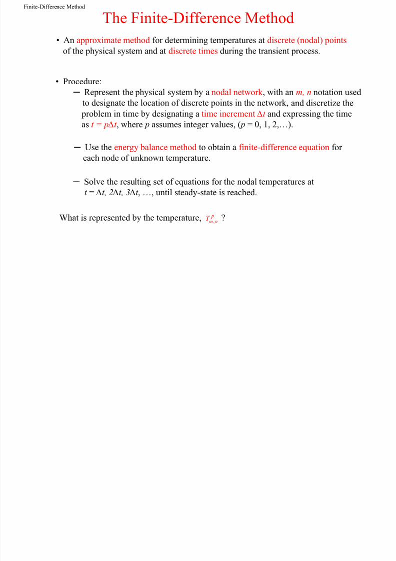
The Finite-Difference Method• An approximate method for determining temperatures at discrete (nodal) points

of the physical system and at discrete times during the transient process.

• Procedure: ─ Represent the physical system by a nodal network , with an m, n notation used

to designate the location of discrete points in the network,

─ Use the energy balance method to obtain a finite-difference equation foreach node of unknown temperature.

─ Solve the resulting set of equations for the nodal temperatures att = ∆t, 2∆t, 3∆t , …, until steady -state is reached.

What is represented by the temperature, ? , p

m nT

and discretize the problem in time by designating a time increment ∆t and expressing the time

as t = p∆t , where p assumes integer values, ( p = 0, 1, 2,…).



Storage Term

Energy Balance and Finite-DifferenceApproximation for the Storage Term

• For any nodal region, the energy balance is

in g st E E E (5.76)

where, according to convention, all heat flow is assumed to be into the region.

• Discretization of temperature variation with time:

• Finite-difference form of the storage term:

1

, ,,

p pm n m n

st m nT T

E ct

• Existence of two options for the time at which all other terms in the energy balance are evaluated: p or p+1 .

1, ,

,

p pm n m n

m n

T T T t t

(5.69)



Explicit Method

The Explicit Method of Solution• All other terms in the energy balance are evaluated at the preceding time

corresponding to p. Equation (5.69) is then termed a forward-differenceapproximation .

• Example: Two-dimensional conductionfor an interior node with ∆x=∆y.

1, ,1, 1, , 1 , 1 1 4 p p p p p p

m n m nm n m n m n m nT Fo T T T T Fo T (5.71)

2 finite-difference form o Four f ier number t Fo x

• Unknown nodal temperatures at the new time, t = (p+1) ∆t, are determinedexclusively by known nodal temperatures at the preceding time, t = p∆t , hencethe term explicit solution .



Explicit Method (cont.)

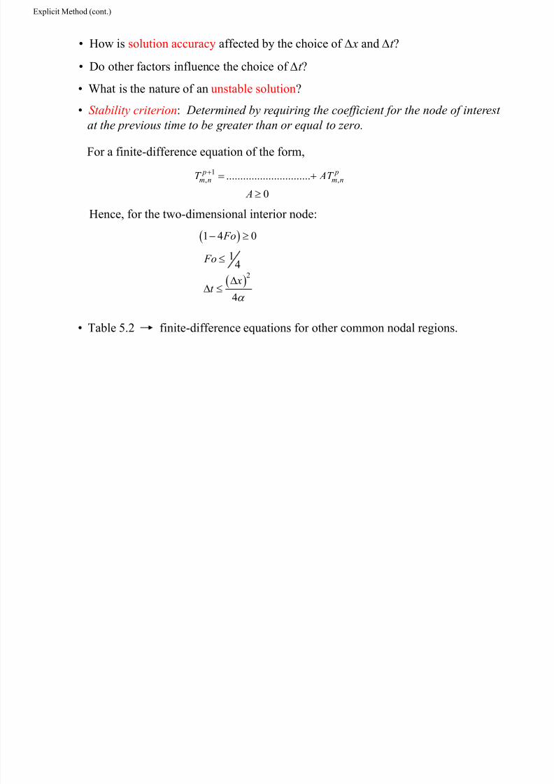
• How is solution accuracy affected by the choice of ∆x and ∆t ?

• Do other factors influence the choice of ∆t ?

• What is the nature of an unstable solution ?• Stability criterion : Determined by requiring the coefficient for the node of interest

at the previous time to be greater than or equal to zero.

1, ,..............................0

p pm n m nT AT A

Hence, for the two-dimensional interior node:

1 4 0 Fo

14 Fo 2

4

xt

• Table 5.2 finite-difference equations for other common nodal regions.

For a finite-difference equation of the form,



Implicit Method

The Implicit Method of Solution• All other terms in the energy balance are evaluated at the new time corresponding

to p+1 . Equation (5.69) is then termed a backward-difference approximation.

• Example: Two-dimensional conduction foran interior node with ∆x=∆y .

1 1 1 1 1, ,1, 1, , 1 , 11 4 p p p p p p

m n m nm n m n m n m n Fo T Fo T T T T T (5.87)

• System of N finite-difference equations for N unknown nodal temperaturesmay be solved by matrix inversion or Gauss-Seidel iteration .

• Solution is unconditionally stable .

• Table 5.2 finite-difference equations for other common nodal regions.



Problem: Finite-Difference Equation

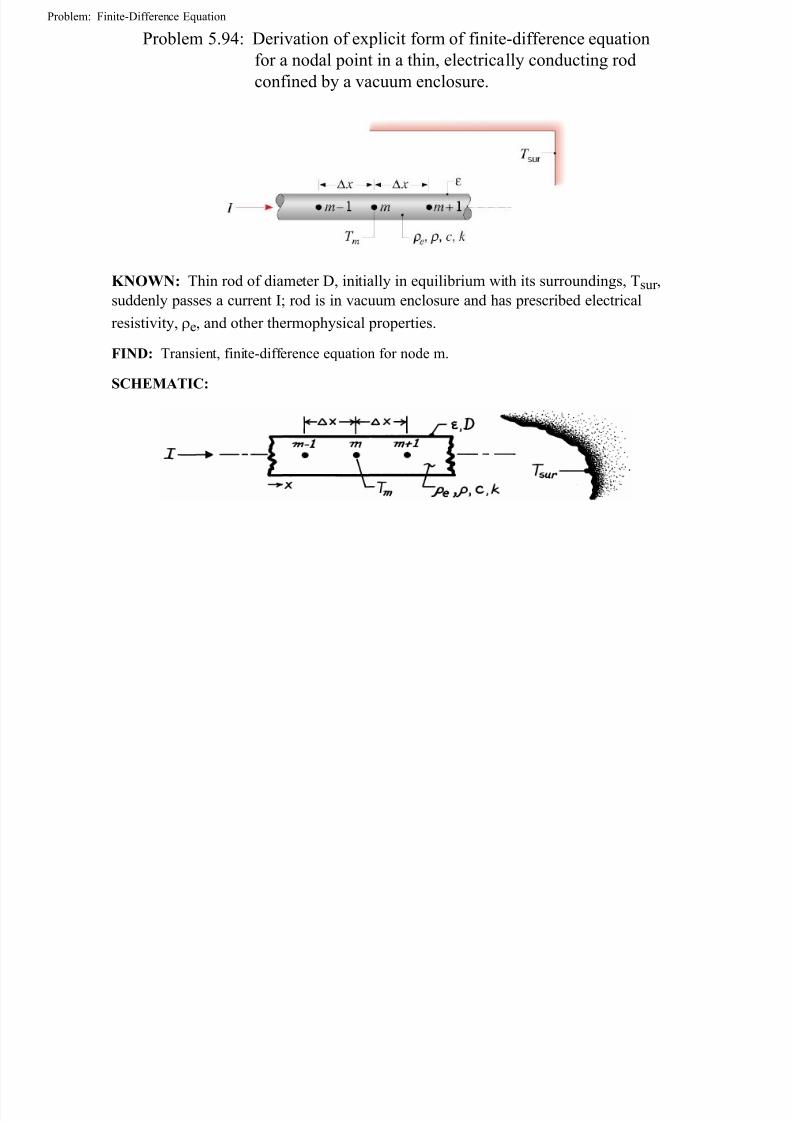
Problem 5.94: Derivation of explicit form of finite-difference equationfor a nodal point in a thin, electrically conducting rodconfined by a vacuum enclosure.

KNOWN: Thin rod of diameter D, initially in equilibrium with its surroundings, T sur ,suddenly passes a current I; rod is in vacuum enclosure and has prescribed electricalresistivity, e, and other thermophysical properties.

FIND: Transient, finite-difference equation for node m.

SCHEMATIC:




ASSUMPTIONS: (1) One-dimensional, transient conduction in rod, (2) Surroundings aremuch larger than rod, (3) Constant properties.

ANALYSIS: Applying conservation of energy to a nodal region of volume cA x,

where2

cA D / 4,

in out g stE E E E

p+1 p2 m m

a b rad eT T

q q q I R cVt

Hence, with 2g eE I R , where e e cR x/A , and use of the forward-difference

representation for the time derivative,

4 p p p p p+1 p4m m p 4 2 em-1 m+1 m m

c c m sur cc

T T T T x T TkA kA D x T T I cA x .

x x A t

Dividing each term by cAc x/ t and solving for p+1mT ,

p+1 p p pm mm-1 m+12 2

k t k tT T T 2 1 T

c cx x

24 p 4 e

m sur 2c c

IP t tT T .

A c cA




or, with Fo = t/ x2,

2 22 4 p+1 p p p p 4 e

m m m sur m-1 m+1 2c c

I xP x

T Fo T T 1 2 Fo T Fo T T Fo.kA kA

Basing the stability criterion on the coefficient of the pmT term, it would follow that

Fo ½.

However, stability is also affected by the nonlinear term, 4 p

mT , and smaller values of Fo may beneeded to insure its existence.



Problem: Cold Plate

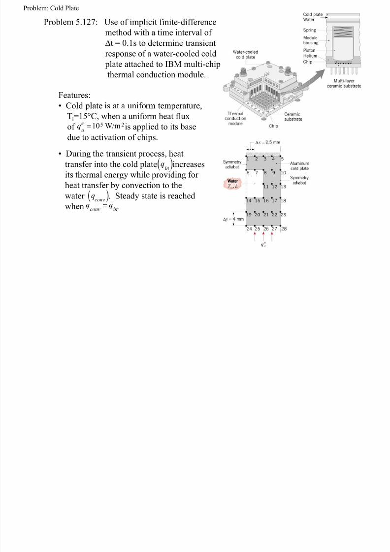
Problem 5.127: Use of implicit finite-differencemethod with a time interval of∆t = 0.1s to determine transientresponse of a water-cooled cold

plate attached to IBM multi-chipthermal conduction module.

Features:• Cold plate is at a uniform temperature,

Ti=15 °C, when a uniform heat fluxof is applied to its basedue to activation of chips.

5 210 W/moq

• During the transient process, heattransfer into the cold plate increasesits thermal energy while providing for

heat transfer by convection to thewater . Steady state is reachedwhen .

inq

convq

conv inq q



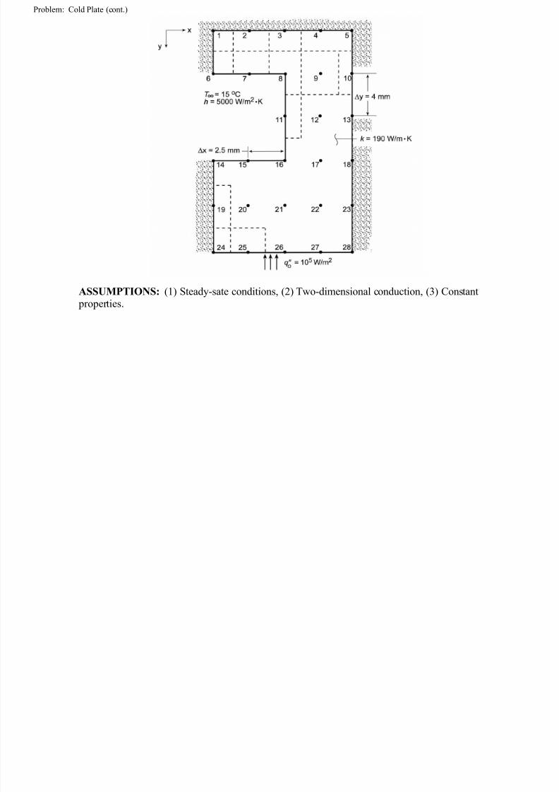
Problem: Cold Plate (cont.)

ASSUMPTIONS: (1) Steady-sate conditions, (2) Two-dimensional conduction, (3) Constant properties.




ANALYSIS:

Nodes 1 and 5:

p+1 p+1 p+1 p1 2 6 12 2 2 2

2 t 2 t 2 t 2 t1 T T T T

x y x y

p+1 p+1 p+1 p5 54 102 2 2 2

2 t 2 t 2 t 2 t1 T T T T

x y x y

Nodes 2, 3, 4:

p+1 p+1 p+1 p+1 pm,n m,nm-1,n m+1,n m,n-12 2 2 2 22 t 2 t t t 2 t1 T T T T Tx y x x y

Nodes 6 and 14:

p+1 p+1 p+1 p76 1 62 2 2 2

2 t 2 t 2h t 2 t 2 t 2h t1 T T T T +T

k y k yx y y x

p+1 p+1 p+1 p14 15 19 142 2 2 2

2 t 2 t 2h t 2 t 2 t 2h t1 T T T T +T

k y k yx y x y




Nodes 7 and 15:

p+1 p+1 p+1 p+1 p7 72 6 82 2 2 2 2

2 t 2 t 2h t 2 t t t 2h t1 T T T T T +T

k y k yx y y x k x

p+1 p+1 p+1 p+1 p15 14 16 20 152 2 2 2 2

2 t 2 t 2h t t t 2 t 2h t1 T T T T T +T

k y k yx y x x y

Nodes 8 and 16:

p+1 p+1 p+178 32 2 2 2

p+1 p+1 p9 11 82 2

2 t 2 t h t t t1 T T Tk xx y y x

4 t 2 t 2 h t 1 1 T T T T

3 3 3 k x yx y

2 2 h t 4 23 3 k y 3 3

p+1 p+1 p+116 11 152 2 2 2

p+1 p+1 p17 21 162 2

2 t 2 t h t t t1 T T T

k xx y y x4 t 4 t 2 h t 1 1

T T T T3 3 3 k x yx y

2 2 h t 2 23 3 k y 3 3




Node 11:

p+1 p+1 p+1 p+1 p11 8 12 16 112 2 2 2 2

2 t 2 t 2h t t t t 2h t1 T T 2 T T T +T

k x k xx y y x y

Nodes 9, 12, 17, 20, 21, 22:

p+1 p+1 p+1 p+1 p+1 pm,n m,nm,n+1 m,n-1 m-1,n m+1,n2 2 2 2

2 t 2 t t t1 T T T T T T

x y y x

Nodes 10, 13, 18, 23:

p+1 p+1 p+1 p+1 pm,n m,nm,n+1 m,n-1 m-1,n2 2 2 22 t 2 t t 2 t1 T T T T Tx y y x

Node 19:

p+1 p+1 p+1 p+1 p19 14 24 20 192 2 2 2

2 t 2 t t 2 t1 T T T T T

x y y x

Nodes 24, 28:

p+1 p+1 p+1 po24 19 25 242 2 2 2

2q t2 t 2 t 2 t 2 t1 T T T +T

k yx y y x

p+1 p+1 p+1 po28 23 27 282 2 2 2

2q t2 t 2 t 2 t 2 t1 T T T +T

k yx y y x




Nodes 25, 26, 27:

p+1 p+1 p+1 p+1 p+1om,n m,nm,n+1 m-1,n m+1,n2 2 2 2

2q t2 t 2 t 2 t t1 T T T T +T

k yx y y x

The convection heat rate per unit length is

conv 6 7 8 11

16 15 14 out.

q h x/2 T T x T T x y T T / 2 y T T xy T T / 2 x T T x/2 T T q

The heat input per unit length is

in oq q 4 x

On a percentage basis, the ratio of convection to heat in is

conv inn q / q 100.




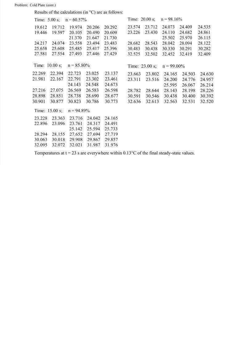
Results of the calculations (in C) are as follows:

Time: 5.00 s; n = 60.57%

19.612 19.712 19.974 20.206 20.29219.446 19.597 20.105 20.490 20.609

21.370 21.647 21.73024.217 24.074 23.558 23.494 23.48325.658 25.608 25.485 25.417 25.39627.581 27.554 27.493 27.446 27.429

Time: 10.00 s; n = 85.80%

22.269 22.394 22.723 23.025 23.13721.981 22.167 22.791 23.302 23.461

24.143 24.548 24.67327.216 27.075 26.569 26.583 26.59828.898 28.851 28.738 28.690 28.67730.901 30.877 30.823 30.786 30.773

Time: 15.00 s; n = 94.89%

23.228 23.363 23.716 24.042 24.16522.896 23.096 23.761 24.317 24.491

25.142 25.594 25.73328.294 28.155 27.652 27.694 27.71930.063 30.018 29.908 29.867 29.85732.095 32.072 32.021 31.987 31.976

Time: 20.00 s; n = 98.16%

23.574 23.712 24.073 24.409 24.53523.226 23.430 24.110 24.682 24.861

25.502 25.970 26.11528.682 28.543 28.042 28.094 28.12230.483 30.438 30.330 30.291 30.28232.525 32.502 32.452 32.419 32.409

Time: 23.00 s; n = 99.00%

23.663 23.802 24.165 24.503 24.63023.311 23.516 24.200 24.776 24.957

25.595 26.067 26.21428.782 28.644 28.143 28.198 28.22630.591 30.546 30.438 30.400 30.39232.636 32.613 32.563 32.531 32.520

Temperatures at t = 23 s are everywhere within 0.13 C of the final steady-state values.

2d heat conduction

Documents