2d ﬂexural backstripping of extensional basins: the … ﬂexural backstripping of extensional...

2D flexural backstripping of extensional basins: the need for asideways glance

Alan M. Roberts1, Nick J. Kusznir2, Graham Yielding1 and Peter Styles2

1Badley Earth Sciences Ltd, North Beck House, North Beck Lane, Hundleby, Spilsby, Lincs, PE23 5NB, UK2Department of Earth Sciences, University of Liverpool, Liverpool, L69 3BX, UK

ABSTRACT: Backstripping is a technique employed to analyse the subsidencehistory of extensional basins, and involves the progressive removal of sedimentloads, incorporating the isostatic and sediment decompaction responses to thisunloading. The results of backstripping calculations using 1D models employinglocal (Airy) isostasy and 2D models employing ‘flexural’ isostasy are compared forthree cross-sections of the North Sea rift basin. Backstripping is commonly used toestimate stretching factor (â) across extensional basins. At structural highs 1D Airybackstripping will overestimate â by comparison with predictions from 2D flexuralbackstripping, because Airy isostasy fails to acknowledge the effects of lateraldifferential loading. Predictions of â from 2D flexural backstripping are closer tothose derived from forward modelling. 1D Airy backstripping also producesunrealistic internal deformation of individual fault-blocks and overestimates â whenthe pre-rift sequence is not fully decompacted.

The palaeobathymetric data required by 1D Airy backstripping are ofteninaccurate, which yields misleading results. 2D flexural backstripping has beenformulated as reverse post-rift modelling, which is used to produce sequential(isostatically balanced) palinspastic post-rift cross-sections. These are calibratedusing only high-quality palaeobathymetric data, allowing 2D flexural backstripping tobe used to predict palaeobathymetry away from the calibration points.

KEYWORDS: isostasy, flexure (geology), compaction (geology), subsidence, basin development

INTRODUCTION

The aim of backstripping is to analyse the subsidence history ofa basin by modelling a progressive reversal of the depositionalprocess. While sensu stricto backstripping may be applied to anysedimentary basin (including platforms and foreland basins), itis most commonly applied to extensional basins, where it isused to determine the magnitude of lithosphere stretching frompost-rift subsidence rate (Sclater & Christie 1980). In additionto constraining the magnitude of lithosphere stretching andresulting basement geotherm perturbations for hydrocarbonmaturation modelling, backstripping may also be used to makepredictions about geological features within a basin, such aspalaeobathymetry and palaeotopography, (Roberts et al. 1993b,Kusznir et al. 1995, Nadin & Kusznir 1995, Roberts et al. 1997,Walker et al. 1997).

The backstripping procedure consists first of removing unitsof stratigraphy from the top downwards (hence backstripping).Corrections must also be made for sediment compaction inresponse to burial and for subsidence arising from the isostaticresponse to sediment loading. Palaeobathymetry estimates areneeded in order to constrain or calibrate earlier stages of basinbathymetry. The isostatic response to loading is commonlycalculated assuming Airy (1D ) isostasy. The ‘traditional’approach, by virtue that it was the first to be used (e.g. Steckler& Watts 1978), is to treat isostasy as a one-dimensionalproblem. 2D flexural backstripping was introduced by Watts

et al. (1982). More recently, 3D flexural backstripping has beenimplemented (Watts & Torne 1992, Norris & Kusznir 1993).The fundamental difference between Airy isostasy, used in 1Dmodelling, and flexural isostasy, used in 2D or 3D modelling, isthat in the 1D approach isostatic loads are compensated locally,i.e. immediately beneath the load, while with the flexuralapproach loads are distributed regionally. 3D backstrippingshould provide the most reliable results, however, its generalapplicability is hampered by the volume of detailed stratigraphicdata (maps) needed. Lateral sampling at scales of 1 km or lesscan, however, readily be provided by 2D data (cross-sections)based on interpreted seismic lines.

In extensional basins subsidence histories produced by back-stripping are usually interpreted in terms of the lithospheric-stretching model of McKenzie (1978), in which lithospherestretching gives rise to crustal thinning and elevation of thegeotherm. Typically the McKenzie lithosphere extension modelassumes a rapid period of syn-rift extension, coincident withsurface faulting, followed by a period of slower time-dependentpost-rift subsidence, during which the thermal anomaly, associ-ated with the elevated geotherm from rifting, cools in anexponential manner with a time constant of c. 65 Ma. Thisepisode of post-rift thermal subsidence causes significant sub-sidence of the basin floor for 150–200 Ma after the rift eventitself.

The aim of this paper is to review 1D Airy-isostatic and 2Dflexural-isostatic backstripping techniques and to compare the

Petroleum Geoscience, Vol. 4 1998, pp. 327–338 1354-0793/98/$10.00 ?1998 EAGE/Geological Society, London

results of backstripping three cross-sections from an exten-sional basin using both techniques. From this we aim to showhow 2D backstripping using flexural isostasy produces moresatisfactory geological predictions.

1D BACKSTRIPPING USING AIRY ISOSTASY

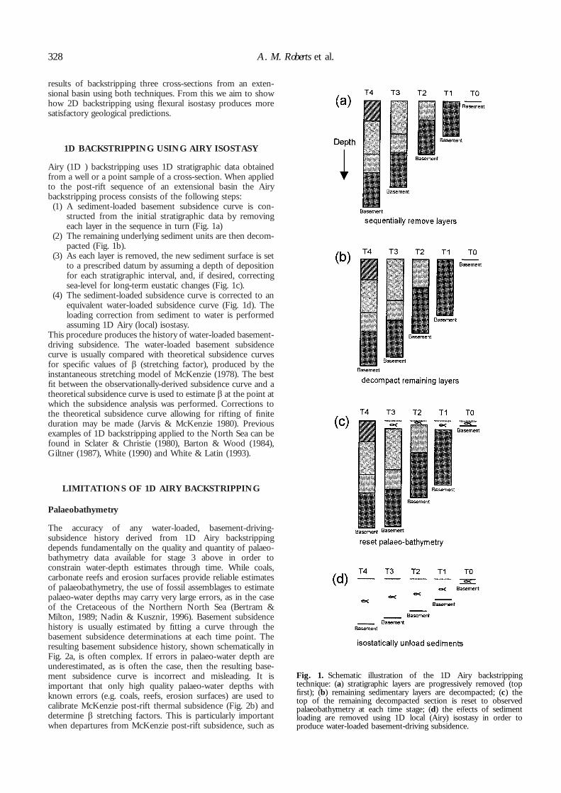
Airy (1D ) backstripping uses 1D stratigraphic data obtainedfrom a well or a point sample of a cross-section. When appliedto the post-rift sequence of an extensional basin the Airybackstripping process consists of the following steps:

(1) A sediment-loaded basement subsidence curve is con-structed from the initial stratigraphic data by removingeach layer in the sequence in turn (Fig. 1a)

(2) The remaining underlying sediment units are then decom-pacted (Fig. 1b).

(3) As each layer is removed, the new sediment surface is setto a prescribed datum by assuming a depth of depositionfor each stratigraphic interval, and, if desired, correctingsea-level for long-term eustatic changes (Fig. 1c).

(4) The sediment-loaded subsidence curve is corrected to anequivalent water-loaded subsidence curve (Fig. 1d). Theloading correction from sediment to water is performedassuming 1D Airy (local) isostasy.

This procedure produces the history of water-loaded basement-driving subsidence. The water-loaded basement subsidencecurve is usually compared with theoretical subsidence curvesfor specific values of â (stretching factor), produced by theinstantaneous stretching model of McKenzie (1978). The bestfit between the observationally-derived subsidence curve and atheoretical subsidence curve is used to estimate â at the point atwhich the subsidence analysis was performed. Corrections tothe theoretical subsidence curve allowing for rifting of finiteduration may be made (Jarvis & McKenzie 1980). Previousexamples of 1D backstripping applied to the North Sea can befound in Sclater & Christie (1980), Barton & Wood (1984),Giltner (1987), White (1990) and White & Latin (1993).

LIMITATIONS OF 1D AIRY BACKSTRIPPING

Palaeobathymetry

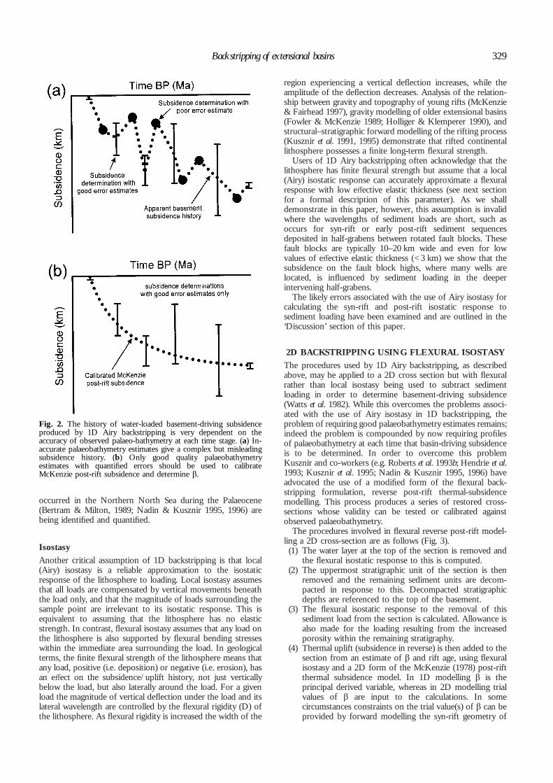
The accuracy of any water-loaded, basement-driving-subsidence history derived from 1D Airy backstrippingdepends fundamentally on the quality and quantity of palaeo-bathymetry data available for stage 3 above in order toconstrain water-depth estimates through time. While coals,carbonate reefs and erosion surfaces provide reliable estimatesof palaeobathymetry, the use of fossil assemblages to estimatepalaeo-water depths may carry very large errors, as in the caseof the Cretaceous of the Northern North Sea (Bertram &Milton, 1989; Nadin & Kusznir, 1996). Basement subsidencehistory is usually estimated by fitting a curve through thebasement subsidence determinations at each time point. Theresulting basement subsidence history, shown schematically inFig. 2a, is often complex. If errors in palaeo-water depth areunderestimated, as is often the case, then the resulting base-ment subsidence curve is incorrect and misleading. It isimportant that only high quality palaeo-water depths withknown errors (e.g. coals, reefs, erosion surfaces) are used tocalibrate McKenzie post-rift thermal subsidence (Fig. 2b) anddetermine â stretching factors. This is particularly importantwhen departures from McKenzie post-rift subsidence, such as

Fig. 1. Schematic illustration of the 1D Airy backstrippingtechnique: (a) stratigraphic layers are progressively removed (topfirst); (b) remaining sedimentary layers are decompacted; (c) thetop of the remaining decompacted section is reset to observedpalaeobathymetry at each time stage; (d) the effects of sedimentloading are removed using 1D local (Airy) isostasy in order toproduce water-loaded basement-driving subsidence.

328 A. M. Roberts et al.

occurred in the Northern North Sea during the Palaeocene(Bertram & Milton, 1989; Nadin & Kusznir 1995, 1996) arebeing identified and quantified.

Isostasy

Another critical assumption of 1D backstripping is that local(Airy) isostasy is a reliable approximation to the isostaticresponse of the lithosphere to loading. Local isostasy assumesthat all loads are compensated by vertical movements beneaththe load only, and that the magnitude of loads surrounding thesample point are irrelevant to its isostatic response. This isequivalent to assuming that the lithosphere has no elasticstrength. In contrast, flexural isostasy assumes that any load onthe lithosphere is also supported by flexural bending stresseswithin the immediate area surrounding the load. In geologicalterms, the finite flexural strength of the lithosphere means thatany load, positive (i.e. deposition) or negative (i.e. erosion), hasan effect on the subsidence/uplift history, not just verticallybelow the load, but also laterally around the load. For a givenload the magnitude of vertical deflection under the load and itslateral wavelength are controlled by the flexural rigidity (D) ofthe lithosphere. As flexural rigidity is increased the width of the

region experiencing a vertical deflection increases, while theamplitude of the deflection decreases. Analysis of the relation-ship between gravity and topography of young rifts (McKenzie& Fairhead 1997), gravity modelling of older extensional basins(Fowler & McKenzie 1989; Holliger & Klemperer 1990), andstructural–stratigraphic forward modelling of the rifting process(Kusznir et al. 1991, 1995) demonstrate that rifted continentallithosphere possesses a finite long-term flexural strength.

Users of 1D Airy backstripping often acknowledge that thelithosphere has finite flexural strength but assume that a local(Airy) isostatic response can accurately approximate a flexuralresponse with low effective elastic thickness (see next sectionfor a formal description of this parameter). As we shalldemonstrate in this paper, however, this assumption is invalidwhere the wavelengths of sediment loads are short, such asoccurs for syn-rift or early post-rift sediment sequencesdeposited in half-grabens between rotated fault blocks. Thesefault blocks are typically 10–20 km wide and even for lowvalues of effective elastic thickness (<3 km) we show that thesubsidence on the fault block highs, where many wells arelocated, is influenced by sediment loading in the deeperintervening half-grabens.

The likely errors associated with the use of Airy isostasy forcalculating the syn-rift and post-rift isostatic response tosediment loading have been examined and are outlined in the‘Discussion’ section of this paper.

2D BACKSTRIPPING USING FLEXURAL ISOSTASY

The procedures used by 1D Airy backstripping, as describedabove, may be applied to a 2D cross section but with flexuralrather than local isostasy being used to subtract sedimentloading in order to determine basement-driving subsidence(Watts et al. 1982). While this overcomes the problems associ-ated with the use of Airy isostasy in 1D backstripping, theproblem of requiring good palaeobathymetry estimates remains;indeed the problem is compounded by now requiring profilesof palaeobathymetry at each time that basin-driving subsidenceis to be determined. In order to overcome this problemKusznir and co-workers (e.g. Roberts et al. 1993b; Hendrie et al.1993; Kusznir et al. 1995; Nadin & Kusznir 1995, 1996) haveadvocated the use of a modified form of the flexural back-stripping formulation, reverse post-rift thermal-subsidencemodelling. This process produces a series of restored cross-sections whose validity can be tested or calibrated againstobserved palaeobathymetry.

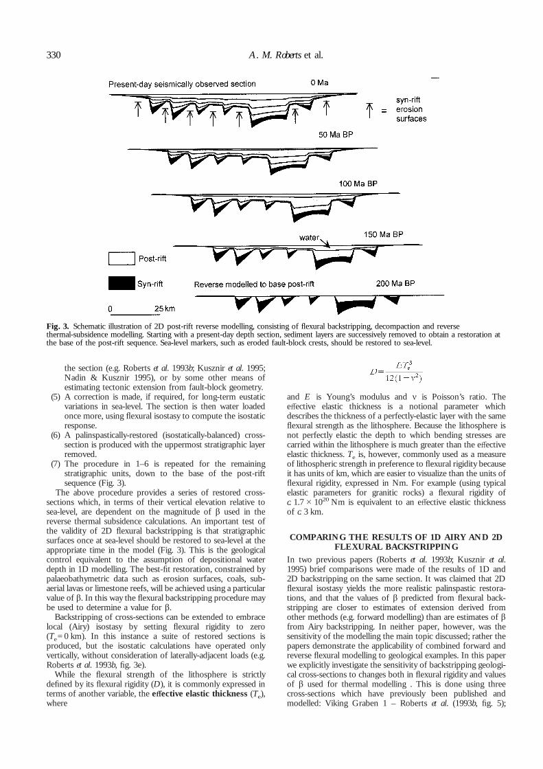
The procedures involved in flexural reverse post-rift model-ling a 2D cross-section are as follows (Fig. 3).

(1) The water layer at the top of the section is removed andthe flexural isostatic response to this is computed.

(2) The uppermost stratigraphic unit of the section is thenremoved and the remaining sediment units are decom-pacted in response to this. Decompacted stratigraphicdepths are referenced to the top of the basement.

(3) The flexural isostatic response to the removal of thissediment load from the section is calculated. Allowance isalso made for the loading resulting from the increasedporosity within the remaining stratigraphy.

(4) Thermal uplift (subsidence in reverse) is then added to thesection from an estimate of â and rift age, using flexuralisostasy and a 2D form of the McKenzie (1978) post-riftthermal subsidence model. In 1D modelling â is theprincipal derived variable, whereas in 2D modelling trialvalues of â are input to the calculations. In somecircumstances constraints on the trial value(s) of â can beprovided by forward modelling the syn-rift geometry of

Fig. 2. The history of water-loaded basement-driving subsidenceproduced by 1D Airy backstripping is very dependent on theaccuracy of observed palaeo-bathymetry at each time stage. (a) In-accurate palaeobathymetry estimates give a complex but misleadingsubsidence history. (b) Only good quality palaeobathymetryestimates with quantified errors should be used to calibrateMcKenzie post-rift subsidence and determine â.

Backstripping of extensional basins 329

the section (e.g. Roberts et al. 1993b; Kusznir et al. 1995;Nadin & Kusznir 1995), or by some other means ofestimating tectonic extension from fault-block geometry.

(5) A correction is made, if required, for long-term eustaticvariations in sea-level. The section is then water loadedonce more, using flexural isostasy to compute the isostaticresponse.

(6) A palinspastically-restored (isostatically-balanced) cross-section is produced with the uppermost stratigraphic layerremoved.

(7) The procedure in 1–6 is repeated for the remainingstratigraphic units, down to the base of the post-riftsequence (Fig. 3).

The above procedure provides a series of restored cross-sections which, in terms of their vertical elevation relative tosea-level, are dependent on the magnitude of â used in thereverse thermal subsidence calculations. An important test ofthe validity of 2D flexural backstripping is that stratigraphicsurfaces once at sea-level should be restored to sea-level at theappropriate time in the model (Fig. 3). This is the geologicalcontrol equivalent to the assumption of depositional waterdepth in 1D modelling. The best-fit restoration, constrained bypalaeobathymetric data such as erosion surfaces, coals, sub-aerial lavas or limestone reefs, will be achieved using a particularvalue of â. In this way the flexural backstripping procedure maybe used to determine a value for â.

Backstripping of cross-sections can be extended to embracelocal (Airy) isostasy by setting flexural rigidity to zero(Te=0 km). In this instance a suite of restored sections isproduced, but the isostatic calculations have operated onlyvertically, without consideration of laterally-adjacent loads (e.g.Roberts et al. 1993b, fig. 3e).

While the flexural strength of the lithosphere is strictlydefined by its flexural rigidity (D), it is commonly expressed interms of another variable, the effective elastic thickness (Te),where

and E is Young’s modulus and í is Poisson’s ratio. Theeffective elastic thickness is a notional parameter whichdescribes the thickness of a perfectly-elastic layer with the sameflexural strength as the lithosphere. Because the lithosphere isnot perfectly elastic the depth to which bending stresses arecarried within the lithosphere is much greater than the effectiveelastic thickness. Te is, however, commonly used as a measureof lithospheric strength in preference to flexural rigidity becauseit has units of km, which are easier to visualize than the units offlexural rigidity, expressed in Nm. For example (using typicalelastic parameters for granitic rocks) a flexural rigidity ofc. 1.7#1020 Nm is equivalent to an effective elastic thicknessof c. 3 km.

COMPARING THE RESULTS OF 1D AIRY AND 2DFLEXURAL BACKSTRIPPING

In two previous papers (Roberts et al. 1993b; Kusznir et al.1995) brief comparisons were made of the results of 1D and2D backstripping on the same section. It was claimed that 2Dflexural isostasy yields the more realistic palinspastic restora-tions, and that the values of â predicted from flexural back-stripping are closer to estimates of extension derived fromother methods (e.g. forward modelling) than are estimates of âfrom Airy backstripping. In neither paper, however, was thesensitivity of the modelling the main topic discussed; rather thepapers demonstrate the applicability of combined forward andreverse flexural modelling to geological examples. In this paperwe explicitly investigate the sensitivity of backstripping geologi-cal cross-sections to changes both in flexural rigidity and valuesof â used for thermal modelling . This is done using threecross-sections which have previously been published andmodelled: Viking Graben 1 – Roberts et al. (1993b, fig. 5);

Fig. 3. Schematic illustration of 2D post-rift reverse modelling, consisting of flexural backstripping, decompaction and reversethermal-subsidence modelling. Starting with a present-day depth section, sediment layers are successively removed to obtain a restoration atthe base of the post-rift sequence. Sea-level markers, such as eroded fault-block crests, should be restored to sea-level.


Viking Graben 2 – White (1990, fig. 11.8); Central Graben –Roberts et al. (1993b, fig. 10). These lines can be geographicallylocated in the earlier papers. For the purposes of this discussiontheir location is not of principal importance.

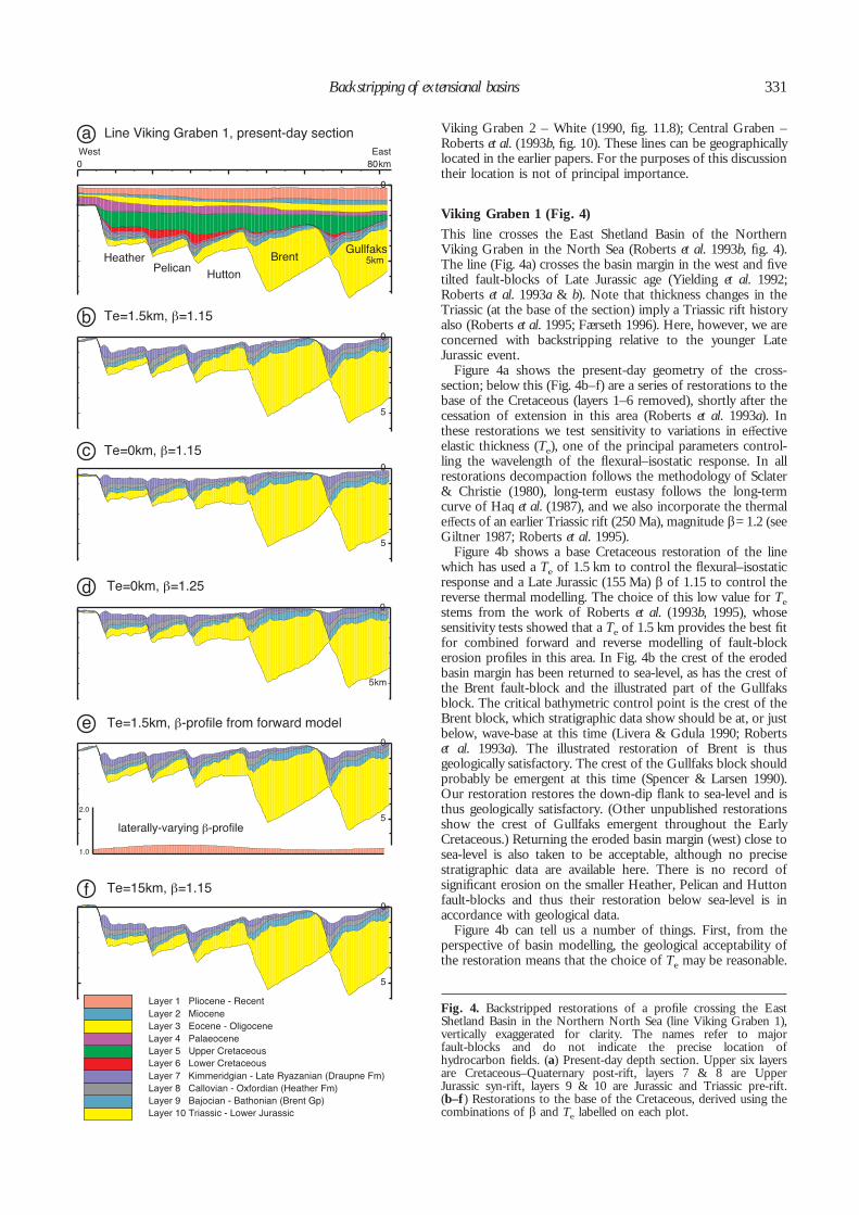
Viking Graben 1 (Fig. 4)

This line crosses the East Shetland Basin of the NorthernViking Graben in the North Sea (Roberts et al. 1993b, fig. 4).The line (Fig. 4a) crosses the basin margin in the west and fivetilted fault-blocks of Late Jurassic age (Yielding et al. 1992;Roberts et al. 1993a & b). Note that thickness changes in theTriassic (at the base of the section) imply a Triassic rift historyalso (Roberts et al. 1995; Færseth 1996). Here, however, we areconcerned with backstripping relative to the younger LateJurassic event.

Figure 4a shows the present-day geometry of the cross-section; below this (Fig. 4b–f) are a series of restorations to thebase of the Cretaceous (layers 1–6 removed), shortly after thecessation of extension in this area (Roberts et al. 1993a). Inthese restorations we test sensitivity to variations in effectiveelastic thickness (Te), one of the principal parameters control-ling the wavelength of the flexural–isostatic response. In allrestorations decompaction follows the methodology of Sclater& Christie (1980), long-term eustasy follows the long-termcurve of Haq et al. (1987), and we also incorporate the thermaleffects of an earlier Triassic rift (250 Ma), magnitude â=1.2 (seeGiltner 1987; Roberts et al. 1995).

Figure 4b shows a base Cretaceous restoration of the linewhich has used a Te of 1.5 km to control the flexural–isostaticresponse and a Late Jurassic (155 Ma) â of 1.15 to control thereverse thermal modelling. The choice of this low value for Testems from the work of Roberts et al. (1993b, 1995), whosesensitivity tests showed that a Te of 1.5 km provides the best fitfor combined forward and reverse modelling of fault-blockerosion profiles in this area. In Fig. 4b the crest of the erodedbasin margin has been returned to sea-level, as has the crest ofthe Brent fault-block and the illustrated part of the Gullfaksblock. The critical bathymetric control point is the crest of theBrent block, which stratigraphic data show should be at, or justbelow, wave-base at this time (Livera & Gdula 1990; Robertset al. 1993a). The illustrated restoration of Brent is thusgeologically satisfactory. The crest of the Gullfaks block shouldprobably be emergent at this time (Spencer & Larsen 1990).Our restoration restores the down-dip flank to sea-level and isthus geologically satisfactory. (Other unpublished restorationsshow the crest of Gullfaks emergent throughout the EarlyCretaceous.) Returning the eroded basin margin (west) close tosea-level is also taken to be acceptable, although no precisestratigraphic data are available here. There is no record ofsignificant erosion on the smaller Heather, Pelican and Huttonfault-blocks and thus their restoration below sea-level is inaccordance with geological data.

Figure 4b can tell us a number of things. First, from theperspective of basin modelling, the geological acceptability ofthe restoration means that the choice of Te may be reasonable.

Fig. 4. Backstripped restorations of a profile crossing the EastShetland Basin in the Northern North Sea (line Viking Graben 1),vertically exaggerated for clarity. The names refer to majorfault-blocks and do not indicate the precise location ofhydrocarbon fields. (a) Present-day depth section. Upper six layersare Cretaceous–Quaternary post-rift, layers 7 & 8 are UpperJurassic syn-rift, layers 9 & 10 are Jurassic and Triassic pre-rift.(b–f ) Restorations to the base of the Cretaceous, derived using thecombinations of â and Te labelled on each plot.


An estimate of Late Jurassic â of 1.15 may also be acceptable.Second, from the geological perspective, the restoration allowsus to make predictions about palaeobathymetry and potentialdepocentres, together with an assessment of which structuresmay, through emergence, have acted as a source for syn-rift/early post-rift reservoir. This would not be possible from 1Dbackstripping of well data.

Figure 4c shows a second base Cretaceous restoration. Theonly difference between the model used here and that ofFig. 4b, is that Te (and thus flexural rigidity) has been set to zero(i.e. Airy isostasy). There are some clear differences betweenFigs 4b & c. In Fig. 4c no part of the section is returned tosea-level and the internal geometry of the fault-blocks haschanged, with much of the differential sea-floor bathymetrypresent in Fig. 4b having been removed.

The internal change of fault-block shape is not thought tomodel a real geological process. It is considered an artefact ofAiry isostasy. Airy isostasy does not acknowledge lateral differ-ential loading and as a consequence results in restorations ofstructural highs (e.g. fault-block crests) which are too deep andrestorations of structural lows which are too shallow, thusremoving much of the internal topography of the fault-blocks.This arises because when finite flexural rigidity is acknowledged(e.g. Fig. 4b) the subsidence history of a given structural high iscontrolled not just by loading from above, it is amplified byloading from the adjacent hanging wall and dip-slope depo-centres. Conversely, the subsidence history of a given structurallow is controlled both by vertical loading from above and thereduced loading on the adjacent structural high and dip-slope.When this lateral loading effect (the ‘sideways glance’ of the titleof this article) is not acknowledged (Airy isostasy) the fault-blocks deform internally (by vertical simple shear) duringrestoration, demonstrating that Airy isostasy is not a realisticmodel of lithosphere loading during post-rift subsidence.

Using 1D sample data (e.g. well data) internal fault-blockdeformation cannot be seen. It is primarily for this reason thatthis shortcoming of 1D backstripping has not previously beenhighlighted.

Figure 4d shows a similar restoration to Fig. 4c, but themagnitude of the Late Jurassic â-factor has been increased to1.25 (i.e. an increase in extension of 66%). In this restorationthe crest of Brent is just below sea-level and the flank ofGullfaks is very slightly emergent. The restoration, however,still suffers from internal deformation of the fault-blocks, andthere is now the question of whether â=1.25 is realistic for thefault geometries on this line.

This question can be answered by forward modelling.Roberts et al. (1993b, fig. 5) illustrated a flexural-cantileverforward model (Kusznir et al. 1991) of this line, matching themodel to a backstripped template. The â-profile produced bythe forward model is shown in Fig. 4e, together with a baseCretaceous restoration which used the â-profile to constrainreverse thermal modelling. Te for this model was 1.5 km.Comparison of Figs 4b & 4e shows them to be similar. This isbecause the â-profile from the forward model encompasses therange 1.1–1.2, the mean value being about 1.15, the constantvalue used to restore Fig. 2b. Most importantly, the forward-modelled â-profile nowhere reaches a value of 1.25, yet this isthe value of â required to restore the crest of Brent, the flankof Gullfaks and the platform margin close to sea-level if Airyisostasy is assumed (Fig. 4d). This suggests that not only is anAiry restoration geometrically inferior to a flexural restorationwith a small-but-finite Te (1.5 km) but that a satisfactorypalaeobathymetric fit is only achieved by using a value of âwhich is not compatible with the fault geometry on the sameline.

Figure 4f is the final base Cretaceous restoration of lineViking Graben 1. As in 4b and 4c a constant â of 1.15 has beenused, but in 4f a large Te of 15 km has constrained flexuralisostasy. This value of Te would correspond to perfect elasticityfor the thickness of the entire upper crustal seismogenic layer innormal continental lithosphere (e.g. Jackson 1987). ComparingFig. 4f with 4b and 4c, it is clear that the geometry of 4f is moresimilar to 4b, the main difference being an increased bathymetryover the central part of the section. We believe the geometryof Fig. 4f to be more acceptable than the Airy restoration inFig. 4c and suggest that while the restoration of this line issensitive to the value of Te, the critical issue is not the exactvalue but whether Te is 0 km or is finite. Iterative modellinghas led us to conclude that a Te of 1.5–3 km provides thebest results in this area. We suggest that a Te of 0 km isunacceptable.

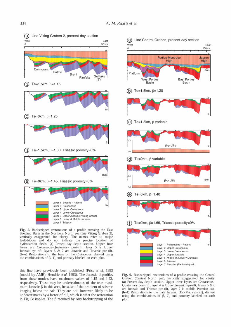
Viking Graben 2 (Fig. 5)

This line also runs c. W–E across the East Shetland Basin,slightly oblique to line Viking Graben 1, intersecting it on theBrent fault-block. This line has previously been used for Airybackstripping by White (1990, see his fig. 2 for location and fig.8 for illustration). Our redisplay of this line (Fig. 5a) is slightlydifferent from White’s original interpretation in that, using theseismic and well data from the area, we have interpreted thelikely top of crystalline basement (base Triassic) (see alsoRoberts et al. 1995; Færseth 1996). White stopped his interpret-ation at the base of the Jurassic. This line is sufficiently close toViking Graben 1 (Fig. 4) that we should expect the results fromanalysis of Viking Graben 1 to be broadly reproducible on thissecond line.

Figure 5b shows Viking Graben 2 backstripped to the base ofthe Cretaceous using a Te of 1.5 km and a Late Jurassic(155 Ma) â of 1.15. In this model, and all others of this line,a Triassic (250 Ma) â of 1.2 is assumed. The controllingparameters on Fig. 5b are thus identical to those of Fig. 4b. Therestoration of the two sections is also similar. In both cases thebasin margin (west) is restored to sea-level, as is the crest ofthe Brent fault-block. The intervening fault-blocks (Cormorant& Hutton in Fig. 5b) are fully submarine in both models. Eastof Brent the crests of the Rimfaks & Gullfaks Sør fault-blocksare restored to sea-level in Fig. 5b. All of the structures atsea-level in Fig. 5b have eroded crests and their restoration tosea-level is therefore consistent with palaeobathymetric infor-mation. There is thus also consistency between two comparableflexural models of lines Viking Graben 1 and 2.

Figure 5c shows Viking Graben 2 backstripped to the baseCretaceous using a Te of 0 km and a constant Late Jurassic of1.25. The controlling parameters are thus the same as forFig. 4d. The crests of the Brent and Rimfaks fault-blocksare restored to sea-level but, as with the Airy models ofViking Graben 1, significant internal deformation of all thefault-blocks has occurred during the reverse modelling. Therestoration in Fig. 5c is less satisfactory than that in Fig. 5b.Flexural isostasy, even with a Te as low as 1.5 km, is required tomaintain the relief between structural highs and lows duringbackstripping.

Figure 4e showed that a â-profile produced by forwardmodelling line Viking Graben 1 is compatible with flexuralbackstripping of the same line, but is incompatible with theAiry backstripped model, the latter requiring higher â values.We have constructed many forward models across the EastShetland Basin. None have produced estimates of Jurassic âexceeding 1.2 and in general â does not exceed 1.15. There is


thus no independent justification for the â of 1.25 required torestore the fault-block crests in Fig. 5c.

White (1990) performed 1D backstripping on six samplepoints from line Viking Graben 2, one from each fault-block. While we estimate a constant â for the profile to bec. 1.15 (Fig. 5b), White estimated the range in Jurassic â to be1.19–1.31, with a mean value of 1.25. This result appearsconsistent with our own Airy backstripping of the line (Fig. 5c).White, however, realized that 1D backstripping yields over-estimates of â when performed on samples from structuralhighs. He therefore sensibly sampled the mid-points of thefault-blocks in an attempt to avoid a structural sampling bias.All other assumptions being the same, Airy backstripping offault-block mid-points should yield similar estimates of â toflexural backstripping, the loading effects of the adjacent highsand lows tending to cancel out. Why then did White obtain anestimate of Jurassic extension c. 66% greater than our own? Thereason lies in the decompaction assumptions. White did notextend his seismic interpretation significantly into the pre-rift,stopping at the top Triassic. He therefore assumed that allpre-Late Jurassic sediments were fully compacted (i.e. hadzero porosity) prior to Late Jurassic extension. This is not aviable assumption in the Northern Viking Graben, because oilis produced from primary porosity in Triassic sandstonereservoirs (e.g. Snorre field, Hollander 1987; Dahl & Solli1993).

Figure 5d shows the effect on backstripping line VikingGraben 2 (Te=1.5 km) when the Triassic is assumed to have noporosity at the beginning of the Cretaceous. In order to restorethe crests of the Brent and Rimfaks fault-blocks to sea-level aLate Jurassic â of 1.3 is required, i.e. the predicted extension istwice that of the flexural model in which the Triassic wasdecompacted (Fig. 5b). We believe this prediction of â to beunsustainable by forward modelling and suggest that theassumptions in the decompaction scheme must be wrong. Weprefer to involve the full sediment column in decompaction,rather than stop decompacting within the pre-rift stratigraphy.This explains why White’s estimates of Jurassic â for this linewere larger than our own.

Figure 5e shows the final restoration of Viking Graben 2.Airy isostasy has been assumed and the Triassic has not beendecompacted. The geometry of the section is highly distortedand in order to restore the crest of the Brent block to sea-levela â of 1.45 is required, an extension estimate (45%) three timesthat of Fig. 5b. This is an unacceptable amount of Jurassicextension for this area and serves to highlight the dangers ofinaccurate geological input during backstripping.

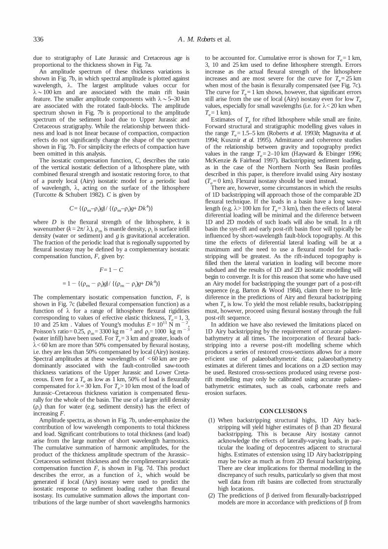
Central Graben (Fig. 6)

This section crosses the Central Graben of the North Sea,c. 400 km south of the previous lines. It was interpreted andforward modelled by Price et al. (1993, fig. 3, located on theirfig. 1) and backstripped by Roberts et al. (1993b, fig. 10). Thesensitivity of this line to assumptions in backstripping has notpreviously been investigated. The line provides a number offeatures to observe during backstripping (Fig. 6a). In thewestern footwall of the Graben is the Forth ApproachesPlatform (Platform on Fig. 6a) and in the eastern footwall is theJæren High; both are thought to be eroded at the base of theCretaceous following footwall uplift on the graben boundaryfaults (Roberts et al. 1990; Price et al. 1993). The Central Grabenitself comprises two Late Jurassic basins, the symmetric WestForties Basin and the asymmetric East Forties Basin, separatedby the eroded Forties–Montrose High. This high is also anuplifted and eroded Late Jurassic footwall (Price et al. 1993,

fig. 4). The aim of backstripping this line is to restore theeroded basin margins and the Forties–Montrose High tosea-level at the time of Late Jurassic extension (c. 155 Ma). TheTriassic locally overlies mobile Zechstein salt which addsstructural complexity to this section not seen in the VikingGraben.

Triassic extension has not been explicitly quantified in thisarea, but the presence of a regionally-thick Triassic sequence inthe Central Graben (e.g. Sørensen 1986; Lervik et al. 1989)suggests that Triassic extension was not negligible. We haveassumed a Triassic â of 1.2, as in our Viking Graben models(see also Roberts et al. 1995). All models incorporate long-termeustasy (after Haq et al. 1987).

The end syn-rift restoration of this line shown in Fig. 6b is aflexural model. It has been backstripped to the base of layer 4(155 Ma) using a Te of 1.5 km and a constant Late Jurassic â of1.2. The eroded platforms flanking the graben are restored tosea-level, but the eroded Forties–Montrose High is left with abathymetry of a few hundred metres. This is rectified in Fig. 6c,which uses a laterally-varying â-profile (1.2 at the margins, 1.3in the centre) to constrain reverse thermal modelling. Thisâ-profile is not constrained by forward modelling, it is simply abest-fit profile for restoring the eroded structures to sea-level.Figure 6c is geologically acceptable.

Although parts of the section are restored to sea-level inFig. 6c, other areas show appreciable bathymetry (>1 km in theEast and West Forties Basins), in which it should have beenpossible to deposit syn-rift reservoir sandstones (Roberts et al.1990; Price et al. 1993). The salt-cored anticlines of the WestForties Basin are also very prominent. These salt structuresgrew during the Late Jurassic, perhaps triggered by extension inthe basement (Roberts et al. 1990) and their relief is probablyexaggerated at the time of the restoration. Nevertheless moni-toring the way in which these short-wavelength/high-amplitudestructures respond to different backstripping assumptions isinformative.

Figure 6d shows a restoration produced using Airy isostasy,with other assumptions the same as Fig. 6c. Nowhere on thissection has been returned to sea-level, indicating that Airybackstripping of the structural highs will require a higher â thanthe comparable flexural model for satisfactory restoration.There are, however, more fundamental differences betweenFigs 6c & 6d, notably the overall geometry of the sections. Airybackstripping has imposed substantial internal deformation ofthe fault-blocks and basins during restoration. The results ofthis are that the East Forties Basin (hanging wall of the JærenHigh) has disappeared, the sea-floor topography in the WestForties Basin has been reduced and the central Forties–Montrose High now lies below the adjacent basinal areas. Thedistortion of the salt-induced topography in the West FortiesBasin has also resulted in deformation of the base-salt/top-basement interface. None of this distortion of internal structureis likely to reflect real geological deformation during post-riftburial, rather it is an artefact of backstripping with Airy isostasy.This would not be apparent if 1D sample data had been used.

Figure 6e shows a second Airy restoration of the CentralGraben line, produced using a constant Jurassic â of 1.4. Thisrestoration still shows internal deformation imposed duringbackstripping, but it does restore the eroded basin margins tosea-level. The ‘penalty’ for this is the much higher value of âthat has been used by comparison with flexural restoration ofthe basin margins. The forward modelling of extension in theCentral Graben is more difficult than in the Viking Graben,because the Permian salt acts to decouple much of thedeformation in the basin fill from true crustal extension in thesub-salt basement. Nevertheless two simple forward models of


this line have previously been published (Price et al. 1993(model by AMR); Hendrie et al. 1993). The Jurassic â-profilesfrom these models have maximum values of 1.15 and 1.23,respectively. These may be underestimates of the true maxi-mum Jurassic â in this area, because of the problem of seismicimaging below the salt. They are not, however, likely to beunderestimates by a factor of c. 2, which is what the restorationin Fig. 6e implies. The â required by Airy backstripping of the

Fig. 5. Backstripped restorations of a profile crossing the EastShetland Basin in the Northern North Sea (line Viking Graben 2),vertically exaggerated for clarity. The names refer to majorfault-blocks and do not indicate the precise location ofhydrocarbon fields. (a) Present-day depth section. Upper fourlayers are Cretaceous–Quaternary post-rift, layer 5 is UpperJurassic syn-rift, layers 6 & 7 are Jurassic and Triassic pre-rift.(b–e) Restorations to the base of the Cretaceous, derived usingthe combinations of â, Te and porosity labelled on each plot.

Fig. 6. Backstripped restorations of a profile crossing the CentralGraben (Central North Sea), vertically exaggerated for clarity.(a) Present-day depth section. Upper three layers are Cretaceous–Quaternary post-rift, layer 4 is Upper Jurassic syn-rift, layers 5 & 6are Jurassic and Triassic pre-rift, layer 7 is mobile Permian salt.(b–f ) Restorations to the Late Jurassic (155 Ma, syn-rift), derivedusing the combinations of â, Te and porosity labelled on eachplot.


structural highs on this line is thus too high to be consistentwith the observed fault-block geometries.

The final restoration of the Central Graben profile (Fig. 6f) issimilar in its construction to the final restoration of line VikingGraben 2 (Fig. 5e). It has been derived using Airy isostasy andwithout decompacting the Triassic. (The salt is not decom-pacted in any restoration). A constant Jurassic â of 1.65 hasbeen used. The Forth Approaches Platform is restored tosea-level, the Forties–Montrose and Jæren Highs are just belowsea-level. There has once more been considerable internaldeformation imposed during the backstripping. The additionalpenalty of the restoration is the unacceptably high â that hasbeen used in order to honour sea-level markers on thestructural highs. At the rift flanks the â of 1.65 implies arequired extension more than three times greater than thatimplied by our preferred flexural model (â=1.2, Fig. 6b & c).

In view of the discussion above, the assumptions used forbackstripping to Fig. 6f might seem unacceptably simple. Thecombined assumptions of Airy isostasy and non-compactingpre-rift are, however, often made in 1D backstripping studies.Figure 6a lies within the bounds of a regional 1D backstrippingstudy in the Central North Sea (White & Latin 1993). TheWhite & Latin study, which used a large number of explorationwells, adopted the assumptions of Airy isostasy and non-compacting pre-rift (Triassic). While the sample of wells in thestudy was selected in order to attempt to avoid a structuralsampling bias, this is unlikely to have been achieved asexploration companies have not drilled structural lows in thisarea. The well-derived 1D data used for this study weretherefore unavoidably biased towards structural highs, some ofwhich are salt cored. In their study of sensitivities White &Latin (fig. 2) demonstrated that ignoring decompaction of the

Triassic in this area can lead to an overestimation of Jurassicextension by as much as 66–100%, much as we have shown. Inthe remainder of their analyses, however, no decompaction ofthe Triassic was performed and yet they argued that theirestimates of Jurassic â were likely minima once all variableswere considered.

In the Central Graben, White & Latin estimated Jurassic âin the graben axis to be in the range 1.5–1.75 (their fig. 9).This range brackets our own estimate of â=1.65, derived fromthe same assumptions (Fig. 6f). We believe this to be anoverestimate of Jurassic â.

DISCUSSION

In this paper we have compared and contrasted the resultsof 1D Airy and 2D flexural backstripping, as applied tothree cross-sections from the North Sea. We believe that 2Dflexural backstripping gives more reliable predictions than thecorresponding 1D Airy backstripping technique. The reasonsfor this are apparent from a spectral analysis of syn-rift andearly post-rift loads across a full transect of the northern VikingGraben.

Lateral variations in the present-day thickness of the syn-rift(Upper Jurassic) and early post-rift (Cretaceous, Upper &Lower) stratigraphic units across a profile from the northernViking Graben are shown in Fig. 7a (see Nadin & Kusznir1995, fig. 11 for original profile). The saw-tooth thicknessvariations, with wavelengths 10–20 km, reflect the control byextensional faulting and rotated fault block geometry on bothLate Jurassic and Early Cretaceous deposition. The total widthof the rift system is of the order of 200 km. Basin fill generatesan isostatic response by sediment loading; the sediment load

Fig. 7. Analysis of the spectral contentof syn-rift and early post-rift sedimentloading and its flexural isostaticresponse. (a) Thickness profile ofUpper Jurassic (syn-rift) and Cretaceous(early post-rift) across the North VikingGraben. (b) Amplitude spectrum ofUpper Jurassic–Cretaceous thickness asa function of wavelength. (c) Flexuralcompensation function, F, (also calledcomplementary isostatic compensationfunction, see text) as a function ofwavelength for Te=1, 3, 10 and 25 km.(d) Cumulative summation of harmonicamplitudes for the product of theamplitude spectrum of Upper Jurassicand Cretaceous thickness and thecomplimentary isostatic compensationfunction, F, as a function ofwavelength. This product and itscumulative summation show thesignificant errors arising from the useof local (Airy) isostasy to determine theisostatic response to sediment loading.Flexural isostasy should be used instead.


due to stratigraphy of Late Jurassic and Cretaceous age isproportional to the thickness shown in Fig. 7a.

An amplitude spectrum of these thickness variations isshown in Fig. 7b, in which spectral amplitude is plotted againstwavelength, ë. The largest amplitude values occur forë2100 km and are associated with the main rift basinfeature. The smaller amplitude components with ë25–30 kmare associated with the rotated fault-blocks. The amplitudespectrum shown in Fig. 7b is proportional to the amplitudespectrum of the sediment load due to Upper Jurassic andCretaceous stratigraphy. While the relationship between thick-ness and load is not linear because of compaction, compactioneffects do not significantly change the shape of the spectrumshown in Fig. 7b. For simplicity the effects of compaction havebeen omitted in this analysis.

The isostatic compensation function, C, describes the ratioof the vertical isostatic deflection of a lithosphere plate, withcombined flexural strength and isostatic restoring force, to thatof a purely local (Airy) isostatic model for a periodic loadof wavelength, ë, acting on the surface of the lithosphere(Turcotte & Schubert 1982). C is given by

C={(ñm–ñi)g}/{(ñm–ñi)g+Dk4)}

where D is the flexural strength of the lithosphere, k iswavenumber (k=2ð/ë), ñm is mantle density, ñi is surface infilldensity (water or sediment) and g is gravitational acceleration.The fraction of the periodic load that is regionally supported byflexural isostasy may be defined by a complementary isostaticcompensation function, F, given by:

F=1"C

=1"{(ñm"ñi)g}/{(ñm"ñi)g+Dk4)}

The complementary isostatic compensation function, F, isshown in Fig. 7c (labelled flexural compensation function) as afunction of ë for a range of lithosphere flexural rigiditiescorresponding to values of effective elastic thickness, Te=1, 3,10 and 25 km . Values of Young’s modulus E=1011 N m"2,Poisson’s ratio=0.25, ñm=3300 kg m"3 and ñi=1000 kg m"3

(water infill) have been used. For Te=3 km and greater, loads ofë<60 km are more than 50% compensated by flexural isostasy,i.e. they are less than 50% compensated by local (Airy) isostasy.Spectral amplitudes at these wavelengths of <60 km are pre-dominantly associated with the fault-controlled saw-tooththickness variations of the Upper Jurassic and Lower Creta-ceous. Even for a Te as low as 1 km, 50% of load is flexurallycompensated for ë=30 km. For Te>10 km most of the load ofJurassic–Cretaceous thickness variation is compensated flexu-rally for the whole of the basin. The use of a larger infill density(ñi) than for water (e.g. sediment density) has the effect ofincreasing F.

Amplitude spectra, as shown in Fig. 7b, under-emphasize thecontribution of low wavelength components to total thicknessand load. Significant contributions to total thickness (and load)arise from the large number of short wavelength harmonics.The cumulative summation of harmonic amplitudes, for theproduct of the thickness amplitude spectrum of the Jurassic–Cretaceous sediment thickness and the complimentary isostaticcompensation function F, is shown in Fig. 7d. This productdescribes the error, as a function of ë, which would begenerated if local (Airy) isostasy were used to predict theisostatic response to sediment loading rather than flexuralisostasy. Its cumulative summation allows the important con-tributions of the large number of short wavelengths harmonics

to be accounted for. Cumulative error is shown for Te=1 km,3, 10 and 25 km used to define lithosphere strength. Errorsincrease as the actual flexural strength of the lithosphereincreases and are most severe for the curve for Te=25 kmwhen most of the basin is flexurally compensated (see Fig. 7c).The curve for Te=1 km shows, however, that significant errorsstill arise from the use of local (Airy) isostasy even for low Tevalues, especially for small wavelengths (i.e. for ë<20 km whenTe=1 km).

Estimates of Te for rifted lithosphere while small are finite.Forward structural and stratigraphic modelling gives values inthe range Te=1.5–5 km (Roberts et al. 1993b; Magnavita et al.1994; Kusznir et al. 1995). Admittance and coherence studiesof the relationship between gravity and topography predictvalues in the range Te=2–10 km (Hayward & Ebinger 1996;McKenzie & Fairhead 1997). Backstripping sediment loading,as in the case of the Northern North Sea Basin profilesdescribed in this paper, is therefore invalid using Airy isostasy(Te=0 km). Flexural isostasy should be used instead.

There are, however, some circumstances in which the resultsof 1D backstripping will approach those of the comparable 2Dflexural technique. If the loads in a basin have a long wave-length (e.g. ë>100 km for Te=3 km), then the effects of lateraldifferential loading will be minimal and the difference between1D and 2D models of such loads will also be small. In a riftbasin the syn-rift and early post-rift basin floor will typically beinfluenced by short-wavelength fault-block topography. At thistime the effects of differential lateral loading will be at amaximum and the need to use a flexural model for back-stripping will be greatest. As the rift-induced topography isfilled then the lateral variation in loading will become moresubdued and the results of 1D and 2D isostatic modelling willbegin to converge. It is for this reason that some who have usedan Airy model for backstripping the younger part of a post-riftsequence (e.g. Barton & Wood 1984), claim there to be littledifference in the predictions of Airy and flexural backstrippingwhen Te is low. To yield the most reliable results, backstrippingmust, however, proceed using flexural isostasy through the fullpost-rift sequence.

In addition we have also reviewed the limitations placed on1D Airy backstripping by the requirement of accurate palaeo-bathymetry at all times. The incorporation of flexural back-stripping into a reverse post-rift modelling scheme whichproduces a series of restored cross-sections allows for a moreefficient use of palaeobathymetric data; palaeobathymetryestimates at different times and locations on a 2D section maybe used. Restored cross-sections produced using reverse post-rift modelling may only be calibrated using accurate palaeo-bathymetric estimates, such as coals, carbonate reefs anderosion surfaces.

CONCLUSIONS

(1) When backstripping structural highs, 1D Airy back-stripping will yield higher estimates of â than 2D flexuralbackstripping. This is because Airy isostasy cannotacknowledge the effects of laterally-varying loads, in par-ticular the loading of depocentres adjacent to structuralhighs. Estimates of extension using 1D Airy backstrippingmay be twice as much as from 2D flexural backstripping.There are clear implications for thermal modelling in thediscrepancy of such results, particularly so given that mostwell data from rift basins are collected from structurallyhigh locations.

(2) The predictions of â derived from flexurally-backstrippedmodels are more in accordance with predictions of â from


forward modelling than are the predictions of 1D Airybackstripped models.

(3) 1D backstripping can only analyse 1D data, such as wellsor vertical stratigraphic samples. 2D backstripping can beused to analyse geological cross-sections.

(4) 1D backstripping yields modelled subsidence curves as itsprimary output. 2D backstripping can also be used toproduce subsidence curves, but its primary output of asequence of palinspastically-restored cross-sections, pre-dicting bathymetry and emergence through the post-rifthistory of a basin, provides more information on the basinevolution than do the simple subsidence curves.

(5) 2D flexural backstripping may be formulated as a reversepost-rift modelling process which produces a series ofisostatically-balanced, restored cross-sections. Theserestored cross-sections are calibrated using only highquality palaeobathymetric estimates, thus providing moreaccurate estimates of â stretching factors.

(6) 1D Airy backstripping, when applied as a series of 1Dsamples across a cross-section, produces unrealistic dis-tortion of internal fault-block geometries, that wouldnot be recognized when isolated samples are analysed.Flexural backstripping maintains the internal geometry offault-blocks.

(7) When incomplete decompaction of the pre-rift stratigra-phy is performed then this too leads to overestimation ofâ, with extension estimates from incomplete decompac-tion being up to twice as large as estimates from a fullydecompacted stratigraphic sequence.

(8) If 1-D Airy backstripping is combined with incompletedecompaction of the pre-rift, then extension estimatesmay be three times larger than those derived from a fullydecompacted flexural model.

(9) Even if Te is low (e.g. the 1.5 km used here) 2D flexuralbackstripping should always be superior in its predictionsto Airy backstripping, because a 2D, rather than 1D,treatment of a 3D problem is being applied. The use of aflexural model is most critical when short-wavelengthtopography or short-wavelength loads are analysed.Flexural and Airy models start to converge when moreregionally distributed loads are considered.

(10) The accuracy of the results of 1D Airy backstripping arevery dependent on the quality of palaeobathymetric esti-mates required by the Airy backstripping process. As aconsequence the predictions of Airy backstripping areoften complex and may produce misleading estimates of âstretching factor.

We thank Kai Sørensen for his review and Tony Spencer for hiseditorial assistance. The corresponding author is Alan Roberts(email: [email protected]).

REFERENCES

BARTON, P. & WOOD, R. 1984. Tectonic evolution of the North Seabasin: crustal stretching and subsidence. Geophysical Journal of the RoyalAstronomical Society, 79, 987–1022.

BERTRAM, G. T. & MILTON, N. J. 1989. Reconstructing basin evolutionfrom sedimentary thickness; the importance of palaeobathymetric control,with reference to the North Sea. Basin Research, 1, 247–257.

DAHL, N. & SOLLI, T. 1993. The structural evolution of the SnorreField and surrounding areas. In: Parker, J. R. (eds) Petroleum Geology ofNorthwest Europe: Proceedings of the 4th Conference. Geological Society, London,1159–1166.

FÆRSETH, R. B. 1996. Interaction of Permo-Triassic and Jurassic exten-sional fault-blocks during the development of the northern North Sea.Journal of the Geological Society, London, 153, 931–944.

FOWLER, S. & McKENZIE, D. P. 1989. Gravity studies of the Rockall andExmouth Plateaux using SEASAT altimetry. Basin Research, 2, 27–34.

GILTNER, J. P. 1987. Application of extensional models to the NorthernViking Graben. Norsk Geologisk Tidsskrift, 67, 339–352.

HAQ, B., HARDENBOL, J. & VAIL, P. R. 1987. Chronology of fluctuatingsea level since the Triassic (250 million years to present). Science, 25,1156–1167.

HAYWARD, N. J. & EBINGER, C. J. 1996. Variations in the along strikesegmentation of the Afar rift system. Tectonics, 15, 244–257.

HENDRIE, D. B., KUSZNIR, N. J. & HUNTER, R. H. 1993. Jurassicextension estimates for the North Sea ‘triple junction’ from flexuralbackstripping: implications for decompression melting models. Earth andPlanetary Science Letters, 116, 113–127.

HOLLANDER, N. B. 1987. Snorre. In: Spencer, A. M. et al. (eds) Geology ofthe Norwegian Oil and Gas Fields. Graham & Trotman, London, 307–318.

HOLLIGER, K. & KLEMPERER, S. L. 1990. Gravity and deep seismicreflection profiles across the North Sea rifts. In: Blundell, D. J. & Gibbs,A. D. (eds) Tectonic Evolution of the North Sea Rifts. Oxford University Press,Oxford, 82–100.

JACKSON, J. A. 1987. Active normal faulting and crustal extension. In:Coward, M. P., Dewey, J. F. & Hancock, P. L. (eds) Continental ExtensionalTectonics. Geological Society, London, Special Publications, 28, 3–17.

JARVIS, G. T. & McKENZIE, D. P. 1980. Sedimentary basin formationwith finite extension rates. Earth and Planetary Science Letters, 48, 42–52.

KUSZNIR, N. J., MARSDEN, G. & EGAN, S. S. 1991. A flexural cantileversimple-shear/pure-shear model of continental lithosphere extension:application to the Jeanne d’Arc Basin and Viking Graben. In: Roberts,A. M., Yielding, G. & Freeman, B. (eds) The Geometry of Normal Faults.Geological Society, London, Special Publications, 56, 41–60.

——, ROBERTS, A. M. & MORLEY, C. 1995. Forward and ReverseModelling of Rift Basin Formation. In: Lambiase, J. (ed.) HydrocarbonHabitat in Rift Basins. Geological Society, London, Special Publications, 80,33–56.

LERVIK, K. S., SPENCER, A. M. & WARRINGTON, G. 1989. Outline ofTriassic stratigraphy and structure in the central and northern North Sea.In: Collinson, J. D. (ed.) Correlation in Hydrocarbon Exploration, (NorwegianPetroleum Society) Graham & Trotman, London, 173–189.

LIVERA, S. E. & GDULA, J. E. 1990. Brent Oil Field. In: Beaumont, E. A.& Foster, N. H. (eds) Atlas of Oil and Gas Fields, Structural Traps II, TrapsAssociated with Tectonic Faulting. American Association of PetroleumGeologists, 21–63.

MAGNAVITA, L. P., DAVISON, I. & KUSZNIR, N. J. 1994. Rifting,erosion and uplift history of the Reconcavo–Tucano–Jatoba Rift, northernBrazil. Tectonics, 13, 367–388.

McKENZIE, D. P. 1978. Some remarks on the development of sedimentarybasins. Earth and Planetary Science Letters, 40, 25–32.

—— & FAIRHEAD, D. 1997. Estimates of the effective elastic thickness ofthe continental lithosphere from Bouguer and free air gravity anomalies.Journal of Geophysical Research, 102, 27 523–27 552.

NADIN, P. A. & KUSZNIR, N. J. 1995. Palaeocene uplift and Eocenesubsidence in the northern North Sea Basin from 2D forward and reversestratigraphic modelling. Journal of the Geological Society, London, 152, 833–848.

—— & —— 1996. Forward and reverse stratigraphic modelling ofCretaceous-Tertiary post-rift subsidence and Palaeogene uplift in the OuterMoray Firth Basin, central North Sea. In: Knox, R. W. O’B., Corfield,R. M. & Dunay, R. E. (eds) Correlation of the Early Palaeogene in NorthwestEurope. Geological Society, London, Special Publications, 101, 43–62.

NORRIS, S. & KUSZNIR, N. J. 1993. 3-D reverse modelling of post-riftextensional basins. Terra Nova, 5, 173–174.

PRICE, J. D., DYER, R., GOODALL, I., McKIE, T., WATSON, P. &WILLIAMS, G. 1993. Effective stratigraphical subdivision of the HumberGroup and the Late Jurassic evolution of the UK Central Graben. In:Parker, J. R. (eds) Petroleum Geology of Northwest Europe: Proceedings of the 4thConference. Geological Society, London, 443–458.

ROBERTS, A. M., LUNDIN, E. R. & KUSZNIR, N. J. 1997. Subsidence ofthe Vøring Basin and the influence of the Atlantic continental margin.Journal of the Geological Society, London, 154, 551–557.

——, PRICE, J. D. & OLSEN, T. S. 1990. Late Jurassic half-graben controlon the siting and structure of hydrocarbon accumulations: UK/NorwegianCentral Graben. In: Hardman, R. F. P. & Brooks, J. (eds) Tectonic EventsResponsible for Britain’s Oil and Gas Reserves. Geological Society, London,Special Publications, 55, 229–258.

——, YIELDING, G. & BADLEY, M. E. 1993a. Tectonic and bathymetriccontrols on stratigraphic sequences within evolving half-graben. In:Williams, G. D. & Dobb, A. (eds) Tectonics and Seismic Sequence Stratigraphy.Geological Society, London, Special Publication, 71, 87–121.

——, ——, KUSZNIR, N. J., WALKER, I. & DORN-LOPEZ, D. 1993b.Mesozoic extension in the North Sea: constraints from flexural back-stripping, forward modelling and fault populations. In: Parker, J. R. (eds)


Petroleum Geology of Northwest Europe: Proceedings of the 4th Conference. TheGeological Society, London, 1123–1136.

——, ——, ——, —— & —— 1995. Quantitative analysis of Triassicextension in the Northern Viking Graben. Journal of the Geological Society,London, 152, 15–26.

SCLATER, J. G. & CHRISTIE, P. A. F. 1980. Continental Stretching: anexplanation of the post mid-Cretaceous subsidence of the Central NorthSea Basin. Journal of Geophysical Research, 85, 3711–3739.

SØRENSEN, K. 1986. Danish Basin subsidence by Triassic rifting on alithosphere cooling background. Nature, 319, 660–663.

SPENCER, A. M. & LARSEN, V. B. 1990. Fault traps in the NorthernNorth Sea. In: Hardman, R. F. P. & Brooks, J. (eds) Tectonic EventsResponsible for Britain’s Oil and Gas Reserves. Geological Society, London,Special Publications, 55, 281–298.

STECKLER, M. S. & WATTS, A. B. 1978. Subsidence of the Atlantic-typecontinental margin off New York. Earth and Planetary Science Letters, 41,1–13.

TURCOTTE, D. L. & SCHUBERT, G. 1982. Geodynamics. Wiley, Chichester.WALKER, I. M., BERRY, K. A., BRUCE, J. R., BYSTØL, L. & SNOW,

J. H. 1997. Structural modelling of regional depth profiles in the Vøring

Basin: implications for the structural and stratigraphic development of theNorwegian passive margin. Journal of the Geological Society, London, 154,537–544.

WATTS, A. B. & TORNEu , M. 1992. Crustal structure and the mechanicalproperties of extended continental lithosphere in the Valencia trough(western Mediterranean). Journal of the Geological Society, London, 149,813–827.

——, KARNER, G. D. & STECKLER, M. S. 1982. Lithospheric flexure andthe evolution of sedimentary basins. Philosophical Transactions of the RoyalSociety, London, 305, 249–281.

WHITE, N. J. 1990. Does the uniform stretching model work in the NorthSea? In: Blundell, D. J. & Gibbs, A. D. (eds) Tectonic Evolution of the North SeaRifts. Oxford University Press, Oxford, 217–240.

—— & LATIN, D. M. 1993. Subsidence analyses from the North Sea ‘triplejunction’. Journal of the Geological Society, London, 150, 473–488.

YIELDING, G., BADLEY, M. E. & ROBERTS, A. M. 1992. The structuralevolution of the Brent Province. In: Morton, A. C., Haszeldine, R. S., Giles,M. R. & Brown, S. (eds) Geology of the Brent Group. Geological Society,London, Special Publications, 61, 27–44.

Received 19 June 1997; revised typescript accepted 13 July 1998.


2d ﬂexural backstripping of extensional basins: the … ﬂexural backstripping of extensional...

Documents