1

2.810 Manufacturing Processes and Systems Quiz #2 Solutions

November 18, 2015

90 minutes

Open book, open notes, calculators, computers with internet off. Please present your work clearly and state all assumptions.

Name: ______________________________

Problems: 1. Gas Shortage 2. Manufacturing Systems 3. Process Control

+ Extra Credit (4 points)

4. Unreliable Machines 5. Literature

/ 15 points / 25 points / 20 points / 25 points / 15 points __________

/ 100 points

2

Problem 1. Gas Shortage (15 points) (a) (7 points) Suppose that all car owners fill up their tanks when they are exactly half full. At

the present time, an average of 6 customers per hour arrive at a single pump gas station. It takes an average of 5 minutes to service a car. Please estimate the total time each car is in the station, including the waiting time, and the number of cars in the queue. You may assume that the time distributions are exponential. We can use the M/M/1 queue model (since we are told that the time distributions are exponential) combined with Little’s Law (𝐿 = 𝜆𝑊) to find the required quantities. Average arrival rate: 𝜆 = 6 !"#$

!!= 0.1 !"#$

!"#

Average service rate: 𝜇 = !

!!"#$!"#

= 0.2 !"#$!"#

Then, from M/M/1 queue, the average number of cars in the queue is: 𝐿 = !

!!!= !.!

!.!!!.!= 1 𝑐𝑎𝑟

From Little’s Law, the average waiting time is: 𝑊 = !

!= !

!.!= 10 𝑚𝑖𝑛

(b) (8 points) Now suppose that MIT changes its mind and decides to divest from fossil fuels.

This causes Exxon Mobil to re-examine their business model and they abruptly decide to stop making gasoline and instead invest in renewables. Suppose this causes a gasoline shortage and panic buying takes place. To model this phenomenon, suppose that all car owners now purchase gas when their tanks are exactly 3/4 full. Now since each car owner is putting less gas into her tank during each visit to the station, we assume that the average service time has been reduced to 4.5 minutes. How has panic buying affected the wait at the gas station and the size of the queue?

The drivers are now filling up when their tanks are ¾ full, which is twice as often as before. Therefore, the arrival rate doubles: Average arrival rate: 𝜆 = 12 !"#$

!!= 0.2 !"#$

!"#

The service rate increases slightly: Average service rate: 𝜇 = !

!.!!"#$!"#

= 0.222 !"#$!"#

As before, using M/M/1 queue and Little’s Law:

𝐿 =𝜆

𝜇 − 𝜆=

0.20.222 − 0.2

= 9 𝑐𝑎𝑟𝑠

𝑊 =𝐿𝜆=

90.2

= 45 𝑚𝑖𝑛 We can see that the both the number of cars in the queue and the waiting time increased significantly.

3

Problem 2. Manufacturing Systems (25 points) Consider the Toyota machining cell as shown in the diagram below. The table provides the walking times, manual times, and machining times for the operations in the cell. The part to be produced is the “toy” part you have seen in class. The manual time/machine time is shown above every process, and each of the walking segments is numbered next to an arrow.

Segment Process Walk (sec) Manual (sec) Machine time

(sec) 1 Raw “L” stock 5 0 0 2 Saw 5 15 50 3 Belt Sander 5 15 30 4 Drill 1” diameter 5 20 40 5 Machine 2 corners 5 20 65 6 Machine semi-circle 5 20 70 7 Deposit finished part 5 0 0 Totals 35 90 255

(a) (5 points) Please estimate the production rate for this cell, as well as the inventory in the

system and the total time in the system for a part. Note that manual time includes loading and unloading parts at the machine. Assume that the raw stock is an extruded “L” shape stock already having the correct dimensions. The production rate is generally dependent on the operator’s total time, unless there is a machine whose operation time is longer than the operator’s total time and thus requires him to wait. Operator time = walking time + manual time = 35 + 90 = 125 seconds This is much larger than any of the machine times, so the production rate of the cell will be dependent on the operator’s time: 𝜆 = !

!"#$%&'$ !"#$= !

!"# != 0.008 !"#$%

!= 0.48 !"#$!

!"#

4

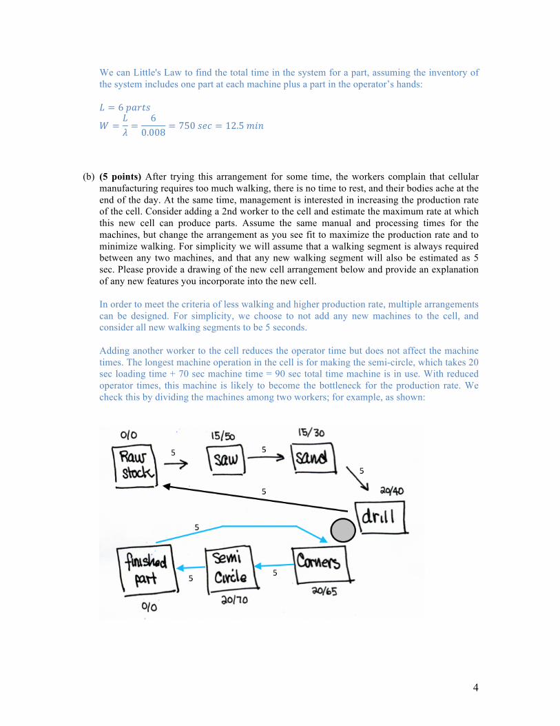
We can Little's Law to find the total time in the system for a part, assuming the inventory of the system includes one part at each machine plus a part in the operator’s hands:

𝐿 = 6 𝑝𝑎𝑟𝑡𝑠

𝑊 =𝐿𝜆=

60.008

= 750 𝑠𝑒𝑐 = 12.5 𝑚𝑖𝑛 (b) (5 points) After trying this arrangement for some time, the workers complain that cellular

manufacturing requires too much walking, there is no time to rest, and their bodies ache at the end of the day. At the same time, management is interested in increasing the production rate of the cell. Consider adding a 2nd worker to the cell and estimate the maximum rate at which this new cell can produce parts. Assume the same manual and processing times for the machines, but change the arrangement as you see fit to maximize the production rate and to minimize walking. For simplicity we will assume that a walking segment is always required between any two machines, and that any new walking segment will also be estimated as 5 sec. Please provide a drawing of the new cell arrangement below and provide an explanation of any new features you incorporate into the new cell. In order to meet the criteria of less walking and higher production rate, multiple arrangements can be designed. For simplicity, we choose to not add any new machines to the cell, and consider all new walking segments to be 5 seconds. Adding another worker to the cell reduces the operator time but does not affect the machine times. The longest machine operation in the cell is for making the semi-circle, which takes 20 sec loading time + 70 sec machine time = 90 sec total time machine is in use. With reduced operator times, this machine is likely to become the bottleneck for the production rate. We check this by dividing the machines among two workers; for example, as shown:

5

Then the times for the two workers, in seconds, are: Worker 1 Worker 2 Walking time 5 + 5 + 5 + 5 = 20 5 + 5 + 5 = 15 Loading time 15 + 15 + 20 = 50 20 + 20 = 40 Total W+L time 20 + 50 = 70 15 + 40 = 55 Max Machine Time Saw: 15 + 50 = 65 Semi-circle: 20 + 70 = 90 As expected, the production rate is limited by the 90-second machine time. Therefore, the overall production rate will be:

𝜆 =190 𝑠

= 0.011 𝑝𝑎𝑟𝑡𝑠𝑠

= 0.667𝑝𝑎𝑟𝑡𝑠𝑚𝑖𝑛

Note that to get this production rate, we would also need to add a buffer where the two workers’ paths meet. Note: All answers that came up with a different design but still demonstrated that the new production rate was higher than in (a) were considered correct.

(c) (5 points) A second option being considered is to incorporate the same processes used in the cell into a transfer line. For the transfer line, the part is attached to a “universal fixture” that is loaded off line. This eliminates the manual loading and unloading time, but adds an operator to load the universal fixture. The transfer line also includes automatic transfer to the next station (which for this exercise we will assume takes no time.). What would be the production rate of the transfer line? The operator can now load the parts off the transfer line, thus eliminating his manual loading time at each machine. The parts are now transferred directly from one machine to the next, so the limiting factor in the production rate is now the longest machining time. From the table provided, the longest machine time is 70 seconds, so the production rate is:

𝜆 =1

𝑀𝑎𝑥 𝑚𝑎𝑐ℎ𝑖𝑛𝑒 𝑡𝑖𝑚𝑒=

170 𝑠

= 0.014 𝑝𝑎𝑟𝑡𝑠𝑠

= 0.86𝑝𝑎𝑟𝑡𝑠𝑚𝑖𝑛

6

(d) (10 points) You need to produce 100,000 of these parts per year, and you are deciding between implementing one of the 3 setups above: cell with 1 worker, cell with 2 workers, or transfer line with one worker to load parts and to monitor the process. The total equipment cost is $100,000 for a cell and $180,000 for a transfer line. The cost of labor is $20 per hour per worker. Which of these manufacturing systems would you choose, based solely on cost? How much does it cost to produce each part? (You can ignore material and any other costs.)

The cost to produce each part is a function of the fixed costs, variable costs, and the number of parts produced. Ignoring material costs, the only variable cost will be the cost of labor:

𝐶!"#$ =𝐹𝑖𝑥𝑒𝑑𝐶𝑜𝑠𝑡𝑁!"#$%

+ 𝑉𝑎𝑟𝐶𝑜𝑠𝑡

𝐶!"#$ =𝐹𝑖𝑥𝑒𝑑𝐶𝑜𝑠𝑡𝑁!"#$%

+ 𝑁!"#$%#&$ℎ𝑟

ℎ𝑟𝑝𝑎𝑟𝑡

𝐶!"#$ =𝐹𝑖𝑥𝑒𝑑𝐶𝑜𝑠𝑡𝑁!"#$%

+ 𝑁!"#$%#&$ℎ𝑟

1𝜆×

13600

ℎ𝑟𝑠

Assume, for instance, that you’re only operating for one year, i.e., you are producing a total of 100,000 parts. Then the production costs for the 3 options are: Cell with 1 worker:

𝐶!"#$ =100,000100,000

+ 1 201

0.008×3600 = 1 + 0.694 = 1.694 $/ 𝑝𝑎𝑟𝑡

Cell with 2 workers, using the production rate found in part (b):

𝐶!"#$ =100,000100,000

+ 2 201

0.011×3600 = 1 + 1.010 = 2.010 $/ 𝑝𝑎𝑟𝑡

Transfer line:

𝐶!"#$ =180,000100,000

+ 1 201

0.014×3600 = 1.8 + 0.397 = 2.197 $/ 𝑝𝑎𝑟𝑡

Based on these results, you would choose the option of the cell with one worker. You could have also compared the options assuming you are operating for longer than a year, i.e., producing more than 100,000 parts. If you plot the three equations with Nparts as the independent variable, you will see that the cost per part for the cell with 2 workers is always higher than for the cell with one worker. However, when producing more than 268,800 parts, the cost per part for the transfer line becomes lower than that for the cell with 1 worker. Note: Your results might vary, depending on the production rate you achieved in part (b).

7

Problem 3. Process Control (20 points) You would like to create a control chart for a process that makes parts to a specific length. You are certain that your process is currently in control, so you take 10 batches of measurements of the length, each batch consisting of n samples. The sample statistics for each batch are provided below (xbar = sample mean, R = sample range, s = sample standard deviation).

Batch xbar R s 1 10.48 0.2 0.084 2 10.38 0.5 0.192 3 10.32 0.5 0.217 4 10.32 0.2 0.084 5 10.30 0.2 0.071 6 10.46 0.4 0.167 7 10.34 0.5 0.207 8 10.48 0.2 0.084 9 10.40 0.4 0.200

10 10.27 0.3 0.134 Average 10.375 0.34 0.144

(a) (5 points) Assuming the number of samples in each batch was n = 5, please calculate the

UCL and LCL of this process. (A table of constants for UCL/LCL equations is included on the last page of the exam.)

We can find the upper and lower control limits using the constants in the chart provided with the values corresponding to n = 5 (5 samples per batch).

𝑥 using 𝑅

𝑥 ± A!R

A2 = 0.5768

𝑥 using 𝑠

𝑥 ± A!s A3 = 1.427

UCL 10.571 10.580 Mean 10.375 LCL 10.179 10.170

You could also calculate the control limits for the range and standard deviation charts (this was not required):

𝑅

D3 = 0, D4 = 2.114

𝑠

B3 = 0, B4 = 2.089 UCL 𝑅𝐷! = 0.000 𝑠𝐵! = 0.000 Mean 𝑅 = 0.340 𝑠 = 0.144 LCL 𝑅𝐷! = 0.719 𝑠𝐵! = 0.301

8

(b) (10 points) Suppose you later take two more batches of 5 samples each, which have the following values:

Batch x1 x2 x3 x4 x5

1 10.41 10.29 10.14 10.17 10.21 2 10.30 10.13 10.12 10.14 10.29

Is the process still in control? Why or why not?

We first find the xbar values for these two batches. They are 10.244 and 10.196, respectively. Comparing these values to the control limits from (a), you can see that both are above the LCL, and thus you could conclude that the process is in control. You could also analyze this a bit deeper and check where the new xbar points fall with respect to the number of standard deviations from the mean. Since we know that the control limits were set to be equal to +/-3σ from the process mean, we can calculate the process standard deviation (or, rather, its estimate) as σ = (UCL - mean)/3 = 0.0654. With this, you could find that the xbar of the first batch falls right on the (mean-2σ) line, while the second one falls outside 2σ from the mean. (This is also clear from the plot below.) This can be a cause for concern, even though the points are still within the control limits.

(c) (5 points) Suppose that all of these measurements are in millimeters (mm). Which

manufacturing process(es) could give you satisfactory results within the control limits from part (a)? Show this by locating these requirements on the figure below.

Using part dimension = 10.375 mm, tolerance = ±0.2 mm, the most appropriate manufacturing processes seem to be investment casting and powder metallurgy.

UCL

LCL

9

Extra Credit (please finish the rest of the exam first!) (d) (4 points) Suppose the original batches actually contained n = 10 samples each, and the 10 samples from part (b) were all taken as one batch (instead of 2 batches of 5 samples). Given this information, is the process still in control? Why or why not? Similarly to part (a) but using different constants for n = 10: xbar (using R)

A2 = 0.3082 xbar (using s) A3 = 0.975

UCL 10.480 10.515 LCL 10.270 10.235

The xbar for the new batch of 10 samples is 10.22. This is below the lower control limit (no matter which method is used to estimate it), so we can conclude that the process is likely to be out of control.

10

Problem 4. Unreliable Machines (25 points) You are making parts on a transfer line consisting of 4 machines. Each machine has a different mean time to failure and mean time to repair, listed in the table (in minutes). The operation time on every machine is 1 minute per part. There is no buffer between any of the machines.

M1 M2 M3 M4 MTTF 500 100 200 250 MTTR 20 10 10 20

(a) (5 points) Assume that machine failures occur as a result of tool breakage, which only happens when the machines are operating. What is the average production rate of the transfer line? This question assumes the operation-dependent failure model, i.e., the machine can only fail when it is operating. Thus, Buzacott’s formula for the production rate of a line with no buffers can be used.

𝑃 =1𝜏

1

1 + 𝑀𝑇𝑇𝑅𝑀𝑇𝑇𝐹

𝑃 = 11

1 + (0.04 + 0.10 + 0.05 + 0.08)= 0.787

𝑝𝑎𝑟𝑡𝑠𝑚𝑖𝑛

(b) (5 points) Assume you are using machines with the same MTTF and MTTR, but now their

failures are caused only by the failure of the control system (which is always on whether or not the machine is operating). What is the average production rate of the transfer line? This problem asks to use a different failure model, i.e. time-dependent failure, rather than operation-dependent failure as in part (a), which was presented on slides 27-29 of the “Time Analysis for Manufacturing Systems” lecture. The equation for production rate with this model is slightly different:

𝑃 =1𝜏𝑃!𝑃!𝑃!𝑃! =

1𝜏

1

1 +𝑀𝑇𝑇𝑅!𝑀𝑇𝑇𝐹!

1

1 +𝑀𝑇𝑇𝑅!𝑀𝑇𝑇𝐹!

1

1 +𝑀𝑇𝑇𝑅!𝑀𝑇𝑇𝐹!

1

1 +𝑀𝑇𝑇𝑅!𝑀𝑇𝑇𝐹!

𝑃 = 11

1.0411.1

11.05

11.08

= 0.9615 0.9091 0.9524 0.9259 = 0.771𝑝𝑎𝑟𝑡𝑠𝑚𝑖𝑛

M1 M2 M3 M4

11

(c) (10 points) You can place one infinite buffer between any two machines. Where would you place it in order to achieve a minimum production rate of 0.85 parts/minute? Assume the original (operation-dependent) failure model applies. You would generally want to place buffers around the bottleneck machine, which in this case is machine 2 (it has the lowest production rate on its own). If we try placing an infinite buffer after this machine, we get a line of machines 1+2 with no buffer, followed by the line of machines 3+4. Using Buzacott’s formula for each of the two lines:

𝑃!,! =1

1 + 0.04 + 0.10=

11.14

= 0.8772𝑝𝑎𝑟𝑡𝑠𝑚𝑖𝑛

𝑃!,! =1

1 + 0.05 + 0.08=

11.13

= 0.8850𝑝𝑎𝑟𝑡𝑠𝑚𝑖𝑛

With the infinite buffer, the production rate of the entire line will be the bottleneck (minimum production rate) among these two parts:

𝑃 = min 𝑃!,!,𝑃!,! = min 0.877, 0.885 = 0.877𝑝𝑎𝑟𝑡𝑠𝑚𝑖𝑛

, which exceeds the requirement of 0.85 parts/minute.

Note: If you place the buffer between machines 1 and 2, you get a production rate of 0.813 parts/min. If you place it between machines 3 and 4, you get a production rate of 0.84 parts/min.

(d) (5 points) Assume the buffer from part (c) is now in place. Please estimate the average number of parts in the buffer. State any assumptions you make.

You can make this estimate using the M/M/1 queue model, with the buffer acting as the system, the production rate of machines 1+2 as the arrival rate (λ), and the production rate of machines 3+4 as the departure rate (µ). With the M/M/1 queue result, the average number of parts is:

𝐿 =𝜆

𝜇 − 𝜆=

0.87720.8850 − 0.8772

= 112 𝑝𝑎𝑟𝑡𝑠

Note, however, that the M/M/1 queue model assumes exponentially-distributed arrival and departure times – this assumption would need to be confirmed. Additionally, if the departure rate was lower than the arrival rate, there would not be a steady-state estimate for the average number of parts in the buffer, as it would keep on growing with time.

12

Problem 5. Literature (15 points) (a) (4 points) According to Maccoby, which jobs are most prized by factory workers?

From Maccoby, page 162: “Even when supervisors have allowed teamwork and opportunities for problem solving and participation (all of which workers appreciate), assembly work remains monotonous and stressful… The jobs most prized by employees are the ones that allow the most autonomy, ranging from high-paying jobs such as programming robots to lower-paying janitorial work.”

(b) (5 points) Please list four reasons explaining why Ford’s changeover from the Model T to the

Model A was so difficult. Hounshell’s Chapter 7 (pp. 280- 292) identifies multiple challenges encountered during the changeover to the Model A in 1927, which required a 6-month complete shutdown of the plant. Some examples: (1) Henry Ford wanted to stop using stampings for the car body and use forgings instead.

Forging was used only minimally on the previous Model T, so most forging capability had been eliminated from the Rouge plant and they were purchased from outside suppliers. This caused procurement delays and a large cost increase.

(2) Delays in design due to disagreements between Ford and his engineers. (3) Ford’s decision to make the gasoline tank integral with the cowl of the Model A, which

caused issues in production with seam welding. (4) Ford decided to increase the precision of all machining work in order to ensure the

highest possible quality for the automobile. Smaller tolerances on most parts required more frequent use of gauging, scaling, and balancing in production and thus more time.

(c) (6 points) Please list three possible sources of waste in a manufacturing system and describe

how the Toyota Production System addressed each one.

Referring to the Monden reading, several sources of waste can be pointed out, such as: (1) excessiveworkforce, (2) excessive inventory, (3) excessive capital investment. The TPS addresses these as follows: (1) Excessive workforce can be eliminated by re-allocating worker operations and ensuring a

flexible multi-functional workforce. (2) Excessive inventory is controller by implementing Just-in-time production, i.e.,

production regulated by the velocity of sales, which is maintained using the pull system. (3) Excessive capital investment can be reduced by eliminating excessive inventory, since

extra inventory requires investment in extra warehouses and additional transport equipment.

13