2.7 astronomy and geophysics - national physical · pdf file2.7 astronomy and geophysics ......

2.7 Astronomy and geophysics

2.7.1 Astronomical and atomic time systems Time systems

The fundamental reference timescale is now international atomic time (TAI). This provides both the standard unit of time (the SI second) and a precise, unambiguous identification of any instant of time, but it is not convenient for general use. There are still valid, practical reasons for continuing to relate the timescalesin general use to the rotation of the Earth by the adoption of a system of standard times each of which differs from that for the prime meridian (zero longitude) by an exact number of hours. The standard time forthe prime meridian is formally known as coordinated universal time (UTC), but the name Greenwich meantime (GMT) is still in widespread use throughout the world. This timescale differs from TAI by an exact number of seconds in such a way that it corresponds closely (to within 1 s) to universal time (UT) and so can be used directly in astronavigation as a measure of the rotation of the Earth with respect to the celestialsphere.

The rotation of the Earth on its axis is no longer of value for the measurement of precise time since the length of the day is subject to unpredictable variations. The systems of sidereal and solar time, includinguniversal time, that represent this rotation are, however, still of value for astronomical purposes and for thedetermination of position on the Earth. These timescales may be regarded as angles expressed in time-units atthe rate of 1 day of 24 hours for each complete rotation (or 1h = 15°).

Precise measurements of the positions of astronomical objects and the corresponding theories of themotions of bodies in the Solar System require the use of the general theory of relativity for the definition of celestial space–time reference frames. The time-like arguments, or scales of coordinate time, that are usedfor such purposes are related to TAI, but they are defined so that they maintain continuity with the earlier scalesof dynamical time and ephemeris time (ET).

International atomic time and coordinated universal time

Independent atomic timescales based on caesium frequency standards were maintained by several nationalorganisations from 1955 onwards, but the standard timescales continued to be based on universal time (UT)until 1972. The second of UT varies and so offsets in the carrier frequencies of the broadcast transmissions and occasional small adjustments in phase were required. In 1967 the General Conference on Weights and Measures (CGPM) adopted the atomic definition of the second as the unit of time interval; the adopted frequency of the chosen caesium transition gave continuity with the previous use of the ephemeris second. In 1971 the CGPM gave formal recognition to the atomic timescale maintained by the Bureau International de l’Heure (BIH) as international atomic time (TAI); the arbitrary epoch of the scale was chosen so that TAI and UT were coincident at 1958 January 1.0.

The International Bureau of Weights and Measures (BIPM) assumed responsibility for TAI on 1988January 1. In forming TAI the BIPM combines the results of comparisons of the primary time-standards of three countries and of about 150 secondary time-standards from 30 countries in an attempt to maintain the uniformity of the scale. Transmissions from satellites of the Global Positioning System (GPS) are the mainintermediary in the comparisons; a precision of 10–20 ns is routinely achieved. The current estimate (1993) of the uniformity of the scale is 1 part in 1013 in frequency so that the accumulated error in epoch is less than 3 µs/year.

The second of TAI is made available directly through the transmissions of coordinated universal time(UTC), which was redefined from the beginning of 1972 as an approximation to UT in which the second markers coincide with those of TAI but the numerical values assigned to them are of an adjacent second of UT. At 0h 00m 00s on 1972 January 1 the difference ∆AT = TAI – UTC was made exactly 10 seconds. ‘Leapseconds’ are added to, or subtracted from, UTC as UT drifts with respect to TAI so that the difference ∆UT = UT – UTC does not normally exceed 0.7 s. The one-second steps are made on the last second of a month,preferably June or December; the date is announced several months in advance on the advice of theInternational Earth Rotation Service. Estimates of the differences ∆UT are often given by coding in the broadcast time signals that are used for the dissemination of time and frequency.

182

Differences ∆AT = TAI – UTC

The table gives the dates of the beginning of the periods during which the differences ∆AT took the values indicated.

Relativistic timescales for astronomy

In the context of the general theory of relativity, international atomic time (TAI) may be regarded as a scale of proper time that is appropriate for use for measurements on the surface of the geoid, the equipotential surface for the Earth that corresponds to mean sea level. In astronomy, however, TAI is not used directly, butinstead a scale known as terrestrial time (TT), which is equal to TAI + 32s.184, is used in order to maintaincontinuity with ephemeris time (ET), which is the timescale of many theories and ephemerides and which provides a uniform timescale before 1955. In addition it is necessary to introduce scales of coordinate time foruse in high-precision theories of the motions of bodies with respect to other space–time reference frames. In particular, scales of geocentric coordinate time (TCG) and barycentric coordinate time (TCB) have been defined for use for motions referred to the centre of the Earth and the barycentre of the Solar System,respectively.

These new scales, (TT, TCG and TCB) were defined in a series of recommendations that were adopted by the International Astronomical Union (IAU) in 1991; they supersede the scales of dynamical time that wererecommended by the IAU in 1976.

Ephemeris time

In general terms, ephemeris time is the independent variable of the differential equations for the motions of theSun, Moon and planets under the influence of their mutual gravitational attractions. Formally, the fundamentalepoch and unit of time interval are defined by the first two terms in an adopted expression for the mean longitude of the Sun, although in practice the timescale is determined indirectly from observations of the Moon.The ephemeris second is equal to the SI second to within the limits of accuracy of its determination, and thescale is such that the relation

ET = TAI + 32s.184

can be used for most purposes when interpolating ephemerides whose argument is ephemeris time.Ephemeris time has been superseded by relativistic timescales for current purposes, but for historical

purposes the concept of ephemeris time is still valid. ET may be regarded as the backward continuation of TAI – 32s.184. Current estimates of the annual-mean values of the differences ∆T between universal time and ephemeris time are given in the following table; the values for the earlier epochs depend critically on the value adopted (in this case – 26''/century2 ) for the tidal term in the expression for the Moon’s mean longitude.

1972 Jan. 1 10 s 1979 Jan. 1 18 s 1991 Jan. 1 26 s1972 July 1 11 s 1980 Jan. 1 19 s 1992 July 1 27 s1973 Jan. 1 12 s 1981 July 1 20 s 1993 July 1 28 s1974 Jan. 1 13 s 1982 July 1 21 s 1994 July 1 29 s1975 Jan. 1 14 s 1983 July 1 22 s1976 Jan. 1 15 s 1985 July 1 23 s1977 Jan. 1 16 s 1988 Jan. 1 24 s1978 Jan. 1 17 s 1990 Jan. 1 25 s

2.7 ASTRONOMY AND GEOPHYSICS 183

184 ASTRONOMY AND GEOPHYSICS 2.7Annual-mean values of AT = ET – UT

ET = UT + ∆T UT = ET – ∆T

Sidereal time

Sidereal time represents the orientation of the celestial system of right ascension with respect to the terrestrialsystem of longitude. Local sidereal time is usually defined as the local hour angle of the equinox (‘First Pointof Aries’). An equivalent definition is that it is the right ascension of the local meridian. The direction of theequinox is the line of intersection of the ecliptic (the mean plane of the Earth’s orbit around the Sun) with theplane of the Earth’s equator; it is used as the zero of right ascension. Sidereal time may be determined by observing stars, whose right ascensions are assumed to be known, as they cross the observer’s meridian. The local sidereal time (LST) at a place differs from Greenwich sidereal time (GST) by the longitude of theplace measured from the Greenwich meridian according to the expression

LST = GST + east longitude

where longitude is measured in time-units at the rate of 15° = l h.The precession of the Earth’s axis of rotation around the pole of the ecliptic causes a slow drift of the

equinox with respect to the stars. Consequently, the mean length of the sidereal day is slightly shorter than the period of rotation of the Earth with respect to an inertial frame. The luni-solar forces acting on the Earthalso cause an oscillatory nutation that is superposed on the precessional drift. It is therefore necessary to distinguish between apparent sidereal time and mean sidereal time, where the latter is free from the quasi-periodic irregularities due to nutation. The obliquity of the ecliptic (the inclination of the ecliptic to theplane of the equator) is also affected by the nutation of the axis of rotation of the Earth. The effects of nutationare computed from an adopted numerical series, the principal terms of which are given on p. 189.

Observations of local sidereal time are also affected by the motion of the axis of rotation with respect to the axis of figure of the Earth. This ‘polar motion’, which also causes variations in the latitudes of the observing site with respect to the celestial equator, is unpredictable and must be determined from observations at two or more sites. Its principal components are an annual term and a ‘Chandler wobble’, whose period is about 427 days; the amplitude of the polar motion is usually less than 0 ''.3, corresponding to a displacement of about 9 m on the surface of the Earth.

Universal time

Universal time (UT) is formally defined in terms of Greenwich mean sidereal time (GMST) by a conventionalexpression (see p. 189) that ensures continuity with past practice and yet frees UT from irregularities that would arise if UT were defined in terms of the hour angle of the Sun. (In effect, UT is equivalent to 12h plusthe Greenwich hour angle of a fictitious mean sun.) Even so, UT does not provide a uniform timescale sincethe rate of rotation of the Earth, and hence the length of the day in SI units, is subject to secular, irregular and quasi-periodic changes due to many different causes. During the course of a year the length of the dayvaries by about 1 ms (i.e. 1 part in 108) about its mean value. During the course of a decade the mean valuemay change by as much as 4 ms. During the course of a millenium the mean value increases by about 20 ms as a result of ‘tidal friction’.

h s s s s

– 500 + 4.9 1600 + 128 1850 + 7 1900 – 3 1950 + 290 2.9 1650 50 1860 8 1910 + 10 1960 33

+ 500 1.5 1700 9 1870 + 2 1920 20 1970 411000 0.6 1750 13 1880 – 6 1930 23 1980 511500 0.1 1800 14 1890 – 7 1940 24 1990 57

UT, polar motion and the geodetic positions of the observing sites are now determined mainly from VLBIobservations of extra-galactic radio sources, from laser ranging to certain artificial satellites and the Moon, andfrom the reception of transmissions from satellites of the Global Positioning System (GPS). The results fromthe various techniques are combined and published by the International Earth Rotation Service, which also publishes the relevant standard constants and models.

Local time and the equation of time

Local mean (solar) time (LMT) differs from UT by the time equivalent of the longitude of the place accordingto the expression

LMT = UT + east longitude.

Local mean time differs from clock time by the time equivalent of the difference in longitude between the placeand the appropriate standard meridian, which may not be the nearest standard meridian. This difference will be1 hour greater when summer (daylight-saving) time is in force. The standard meridians, which differ in longitude by 15°, divide the world into standard time zones, in each of which the time differs from UTC by anintegral number of hours.

The time indicated by a simple sundial is known as local apparent (solar) time and it differs from localmean (solar) time by the so-called equation of time. The average amounts by which apparent solar time is inadvance of mean solar time are indicated in the following table; the actual amounts for a given day may varyby up to 0m.3 from these average values.

Equation of time: apparent time – mean time (minutes)

LMT of transit of Sun = 12h – equation of time.

The principal contributions to the equation of time arise from the eccentricity of the Earth’s orbit and fromthe inclination of the plane of the Earth’s orbit to the plane of the Earth’s equator. The equation of time is givento a precision of about 1m by the expression

+ 7m.6 sin(176°.24 + 0°.9856 d) + 9m.8 sin(198°.82 + 1°.9712 d),

where d is the interval in days from January 0.The directions of the stars at a given time are determined by the local sidereal time, which is equal to

the right ascension of the stars on the meridian. The following table shows the approximate right ascension of the stars that will be due south at 0h LMT (midnight) at the beginning of each month. LST gains on LMT by about 4 minutes each day, so that

LST = LMT + value from table for month + (4 minutes × (day of month – 1),

where LMT is the local clock time plus/minus the correction in time for longitude east/west of the appropriatestandard meridian. The value on a given day of the year varies by up to 4 minutes in a four-year cycle.


m m m m

Jan. 1 –3.3 Apr. 1 –3.8 July 1 –3.8 Oct. 1 +10.415 –9.2 15 0.0 15 –5.9 15 +14.3

Feb. 1 –13.6 May 1 +3.0 Aug. 1 –6.2 Nov. 1 +16.414 –14.3 15 +3.7 15 –4.4 15 +15.3

Mar. 1 –12.4 June 1 +2.0 Sep. 1 +0.1 Dec. 1 +10.915 –8.9 15 –0.4 15 +4.9 15 +4.7

At a given LST the local hour angle (LHA) of a star is given by

LHA = LST – right ascension of star.

Local sidereal time (LST) minus local mean time (LMT) (midnight)

The value of LST – LMT increases by about 4 minutes each day.G.A.Wilkins

Time and frequency signals

Portable atomic clocks of high accuracy are now available and are used to compare standard clocks in differentplaces. But this has the disadvantage that only occasional comparisons are possible. Time and its reciprocal,frequency, are unique among physical quantities in that the magnitude of the units can be disseminated by radio means without the need for travelling standards. A number of countries operate standard time and frequency broadcast services: these are available for use by anyone within range of the transmitters who has a suitable radio receiver. The majority of the transmissions are in the MF and HF bands (see p. 113) and can be received over distances of some thousands of kilometres. But because variable delays occur when signals are propagated via the ionosphere, the full accuracy can be obtained only by a receiver within ground-wave range.

In Britain, the service is provided by the National Physical Laboratory by a 60 kHz signal from the MSFtransmitter at Rugby. This has a carrier derived from an atomic frequency standard, with a stability within ± 2 in 1012 of the nominal frequency. It carries accurate time signals and is related to the national atomic frequency standard at Teddington. Corrections to the radiated frequencies are subsequently available to an accuracy of ± 1 in 1013. The carrier of the BBC broadcast transmitter on 198 kHz at Droitwich is also stabilised.

In the United States, NIST broadcasts time and frequency signals at a number of frequencies in the HFband from WWVB (Colorado) and WWVH (Hawaii). WWVB also broadcasts at 60 kHz. Some other countries, notably Germany and Japan, also have dedicated time and frequency broadcast services.

In addition, there are a number of types of signal broadcast for other purposes which can be used for accurate time comparisons. These include television signals, Loran-C and others. But in recent years most interest has been aroused by the possibility of using signals from satellites. There are a number of systemswhich have been used for time comparisons, but perhaps the one which has received most attention has beenthe US Department of Defense Global Positioning System (GPS) in which the satellites carry atomic clocks.This is a navigation system in which, if you know the time, you can work out where you are from the receivedsignals. But equally, if you know where you are (and where the satellite is) you can determine the time. Manylaboratories have made use of this, but it does have the slight disadvantage of being primarily a military system. In an alternative approach, NPL has recently carried out experiments using signals from direct broadcast satellites (DBS) to compare clocks at distances up to 400 km apart with uncertainties of about 100 ns in time and a few parts in 1014 in frequency. Plans for the intercomparison of national standards via satellite links are now under way.

Clearly, the situation is changing rapidly. Some HF broadcasts have already been abandoned and otherbroadcasts are likely to follow. It is not possible to give here details of facilities which are likely to remain inuse. Anyone wishing to obtain up-to-date information on what is currently available should seek it from theirnational standards laboratory (NPL in Britain).

A.E.Bailey

186 ASTRONOMY AND GEOPHYSICS 2.7

h m h m h m h m

Jan. 1 6 40 Apr. 1 12 34 July 1 18 34 Oct. 1 0 34Feb. 1 8 40 May 1 14 34 Aug. 1 20 34 Nov. 1 2 40Mar. 1 10 34 June 1 16 34 Sep. 1 22 40 Dec. 1 4 40

2.7.2 Astronomical units and constants The IAU and IERS systems of astronomical units and constants

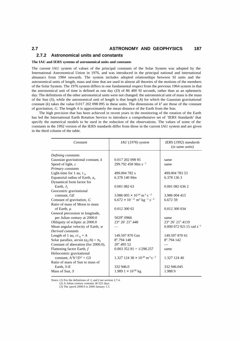
The current IAU system of values of the principal constants of the Solar System was adopted by theInternational Astronomical Union in 1976, and was introduced in the principal national and internationalalmanacs from 1984 onwards. The system includes adopted relationships between SI units and the astronomical units of length, mass and time that are used in almost all theories of the motions of the membersof the Solar System. The 1976 system differs in one fundamental respect from the previous 1964 system in thatthe astronomical unit of time is defined as one day (D) of 86 400 SI seconds, rather than as an ephemeris day. The definitions of the other astronomical units were not changed: the astronomical unit of mass is the massof the Sun (S), while the astronomical unit of length is that length (A) for which the Gaussian gravitational constant (k) takes the value 0.017 202 098 095 in these units. The dimensions of k2 are those of the constant of gravitation, G. The length A is approximately the mean distance of the Earth from the Sun.

The high precision that has been achieved in recent years in the monitoring of the rotation of the Earth has led the International Earth Rotation Service to introduce a comprehensive set of ‘IERS Standards’ that specify the numerical models to be used in the reduction of the observations. The values of some of the constants in the 1992 version of the IERS standards differ from those in the current IAU system and are givenin the third column of the table.


Constant IAU (1976) system IERS (1992) standards(in same units)

Defining constantsGaussian gravitational constant, k 0.017 202 098 95 sameSpeed of light, c 299.792 458 Mm s– 1 samePrimary constantsLight-time for 1 au, τ A 499.004 782 s 499.004 783 53Equatorial radius of Earth, ae 6.378 140 Mm 6.378 136 3Dynamical form factor for

Earth, J2 0.001 082 63 0.001 082 636 2Geocentric gravitational

constant, GE 3.986 005 × 10 14 m 3 s – 2 3.986 004 415Constant of gravitation, G 6.672 × 10 – 11 m3 kg – 1 s – 2 6.672 59Ratio of mass of Moon to mass

of Earth, µ 0.012 300 02 0.012 300 034General precession in longitude,

per Julian century at 2000.0 5029″.0966 sameObliquity of ecliptic at 2000.0 23° 26′ 21″.448 23° 26′ 21″.4119Mean angular velocity of Earth, ω — 0.000 072 92115 rad s–1

Derived constantsLength of 1 au, cτ A = A 149.597 870 Gm 149.597 870 61Solar parallax, arcsin (ae/A) = π 0 8″.794 148 8″.794 142Constant of aberration (for 2000.0), 20″.495 52 —Flattening factor Earth, f 0.003 352 81 = 1/298.257 sameHeliocentric gravitational

constant, A 3k2/D 2 = GS 1.327 124 38 × 10 20 m 3 s – 2 1.327 124 40Ratio of mass of Sun to mass of

Earth, S /E 332 946.0 332 946.045Mass of Sun, S 1.989 1 × 10 30 kg 1.988 9

Notes: (1) For the definitions of J2 and f see section 2.7.4.(2) A Julian century contains 36 525 days.(3) The epoch 2000.0 is 2000 January 1.5.

Other units and the standard epoch

The unit of time in the fundamental formulae for precession (and in similar expressions) is the Julian centuryof 36 525 days (the tropical century is not to be used). The new standard epoch is designated J2000.0 and is the calendar date 2000 January ld.5, which is the Julian date JD 245 1545.0.

An alternative unit for use in Newtonian dynamics of the solar system and binary stars is the Gaussian year, which is the sidereal period of a particle of negligible mass moving around the Sun in an orbit with a mean distance of 1 au; it is equal to 2π/k (= 365.256 898) days. Kepler’s law for the relative motion of two isolated particles of mass M and m is then, simply,

a 3 = P 2(M + m)

where a is the semi-major axis of the orbit in au, P is the period in Gaussian years, and the unit of mass is the mass of the Sun.

A convenient unit for the measurement of the distances of nearby stars is the parsec (pc); this is the distance at which 1 au subtends an angle of 1 second of arc. Hence

1 parsec = l/(sin 1″) au = 2.063 × 10 5 au = 3.086 × 10 16 m

The multiple units kiloparsec (kpc) and megaparsec (Mpc) are more appropriate for most galactic and extragalactic objects respectively. The ‘light-year’ is normally only used in popular astronomical texts:

1 light-year = 0.307 pc = 6.32 × 10 4 au = 9.46 × 10 15 m

Constants relating to time

The following relationships hold in all time systems:

1 day = 24 hours = 1440 minutes = 86 400 seconds1 Julian year = 365.25 days = 8766 hours = 525 960 minutes = 31 557 600 seconds1 century = 100 years

The following values of the lengths of the year, month and day are expressed in units of 1 day of 86 400SI seconds; T is measured in Julian centuries from 2000.0.

1 tropical year (equinox to equinox) = 365d. 242 193 – 0d.000 006 1 T= 365d 05h 48m 45s.5 –0s.53 T

1 sidereal year (fixed star to fixed star) = 365d. 256 360 + 0d. 000 0001 T= 365d 06h 09m 09s. 5 + 0s.01 T

1 mean synodic month (new moon) = 29d. 530 859 = 29d 12h44m02s.91 mean tropical month (equinox) = 27d. 321 582 = 27d 07h43m04s. 71 mean sidereal month (fixed star) = 27d. 321 661 = 27d 07h43m11s.51 mean solar day (current) = ld. 000 000 04 = 86 400s. 0031 mean sidereal day (current) = 0d. 997 269 60 = 86 164s. 0941 mean period of rotation of Earth (current) = 0d. 997 269 70 = 86 164s. 102

The rate of rotation of the Earth is

72 921 151.467 – 0.844 ∆D picoradians/second,

where ∆D is the difference measured in milliseconds between the duration of the mean solar day and 86 400 SIseconds. The current value of ∆D is about 3.

Although the Earth’s period of rotation is variable when measured in SI units the following relationshipsare almost independent of the variability.

1 mean solar day= interval between successive transits of the fictitious mean sun= ld.002 737 909 = 24 h 03m 56 s. 555 3 = 86 636 s. 555 3 of mean sidereal time


1 mean sidereal day= interval between successive transits of the mean equinox= 0d.997 269 566 = 23 h 56m 04 s. 090 5 = 86 164 s. 090 5 of mean solar time

1 period of rotation of the Earth with respect to an inertial reference frame= 1d.000 000 097 = 24 h 00m 00 s. 008 4 = 86 400 s. 008 4 of mean sidereal time= 0d.997 269 663 = 23 h 56m 04 s. 098 9 = 86 164 s. 098 9 of mean solar time

Universal time is related to Greenwich mean sidereal time through the expression:

GMST at 0h UT = 6h 41m 50 s. 548 41 + 8640 184s. 812 866Tu + 0 s. 093 104 T 2u – 6.2 × 10 – 6 T 3

u

where Tu is measured in centuries of 36 525 mean solar days from 2000 January 1 at 12h UT (JD 245 1545.0 UT).

Constants for precession and nutation

The precessional motion of the celestial equator (plane normal to the axis of rotation of the Earth) around the ecliptic (mean plane of the Earth’s orbit around the Sun) has a period of about 25 725 years, and gives rise to the luni-solar precession in celestial longitude of 50″. 37 per year. There is also a slow precessional motion of the ecliptic due to planetary perturbations; this gives both a change in the obliquity (inclination of the ecliptic to the equator) and a motion of the equinox (direction of the line of intersection of equator and ecliptic) along the equator of 0″.12 per year. The combined effect is known as the general precession.

Obliquity of ecliptic = 23° 26' 21″.45 – 46″. 81T = 23°.439 291 – 0°.013 00TAnnual general precession in longitude = 50″. 2910 + 0″. 0222 T

Where T is measured in Julian centuries from 2000.0. For a star with right ascension α and declination δthe annual precessions in right ascension and declination are m + n sin α tan δ and n cos α, respectively, where

m = 3 s. 074 96 + 0s.001 86 T, n = 1s. 336 21 – 0 s. 000 57 T = 20″.0431 – 0″. 0085 T

The nutation of the axis of rotation of the Earth is normally specified by its effects in celestial longitudeand obliquity. The principal terms in the trigonometric series for the nutation are:

References

The Explanatory Supplement to the Astronomical Almanac (ed. P. K. Seidelmann, 1992, University ScienceBooks, Mill Valley, California, ISBN 0-935702-68-7) contains detailed accounts of astronomical time and coordinate systems and of the IAU system of astronomical units and constants.

The IERS Standards (1992) (ed. D. D. McCarthy) have been published as IERS Technical Note 13 by the Central Bureau of the International Earth Rotation Service (Observatoire de Paris, 61 ave de l’Observatoire, F-5014 Paris, France).

G. A. Wilkins


In longitude In obliquity Period (days)

–17 ″. 200 – 0″.017 T +9″.202 + 0″.001 T 6798+0.206 –0.090 3399–1.319 +0.574 183–0.227 +0.098 13.7

2.7.3 The Solar SystemDimensions, etc., of Sun, Moon and planets

Mean elements of the orbits of the planets


Body Equatorial Mass Surface Mean Flattening Period Inclination Numberradius gravity density of of equator of known

(on scale: Earth = 1)† rotation to orbit satellitesMg m– 3

Sun . . . 109.12 332 946 27.96 1.41 0.0 25 d 09 h 7°. —Mercury . 0.382 0.0553 0.38 5.43 0.0 58d 16 h 0°.0 0Venus . . 0.949 0.8150 0.90 5.24 0.0 243 d 00 h 177°.3 0Earth . . 1.000 1.0000 1.00 5.52 0.0034 23 h 56 m 23°.4 1Moon . . 0.272 0.0123 0.17 3.34 See note 4 27 d 08 h 1°.5 —Mars . . 0.532 0.1074 0.38 3.94 0.0052 24 h 37 m 25°.2 2Jupiter . . 11.19 317.89 2.54 1.33 0.0648 9 h 50 m 3°.1 16Saturn . 9.41 95.18 1.07 0.70 0.1076 10 h 14 m 26°.7 18Uranus . 3.98 14.50 0.9 1.30 0.030 15 h 34 m 97°.9 15Neptune . 3.81 17.24 1.2 1.76 0.026 18 h 26 m 29°.6 8Pluto . . 0.23 0.0025 0.05 1.1 0.0 6 d 09 h 117°.6 1

† For Earth values see section 2.7.4.Notes:

(1) The Sun is a star of spectral type G2V and absolute magnitude + 4.79. The effective temperature of its photosphere is about 5800 K. The radiation emitted per unit area is 63.3 MWm – 2, giving a total emission rate of 3.85 × 10 26 W. The radiation received at the Earth under standard conditions (i.e. the solar constant) is 1.37 kW m– 2.

(2) The periods of rotation of the Sun, Jupiter and Saturn refer to their equatorial visual regions; the periods increase with latitude.(3) The inclinations of the equators of the Sun and Moon are referred to the ecliptic; the inclination of the equator of the Moon to the

plane of the Moon’s orbit around the Earth is about 6°.7 and the axis of rotation precesses at the same rate as the line of nodes of the orbit (period 18.6 years).

(4) The mean radius of the Moon may be taken as 1738.0 km, but the irregularities in the surface are of the order of 1/500 of the radius; the principal moments of inertia are all different.

Planet Mean distance Sidereal Synodic Inclination Eccentricity Longitude Longitudefrom Sun period period to ecliptic of node of perihelion

au Gm year day degree degree degree

Mercury . 0.387 57.9 0.241 116 7.005 0.2056 48.3 77.5Venus . . 0.723 108.2 0.615 584 3.394 0.0068 76.7 131.6Earth + Moon 1.000 149.6 1.000 — 0.0 0.0167 — 102.9Mars . . 1.524 227.9 1.881 780 1.850 0.0934 49.6 336.1Jupiter . . 5.203 778.3 11.857 399 1.303 0.0485 100.5 14.3Saturn . . 9.555 1429 29.42 378 2.49 0.055 113.7 93Uranus . 19.22 2875 83.75 370 0.0773 0.046 74.0 173Neptune . 30.11 4504 164 367 1.770 0.009 131.8 48Pluto . . 39.54 5916 248 367 17.13 0.249 110.3 224

Notes:(1) The planetary orbits are subject to both secular and periodic perturbations, so that the osculating elements at any instant may differ

in the end figures from the elements for 2000 that are given above.(2) The values given for Earth + Moon refer to motion of their centre of mass, which lies about 4700 km from the centre of the Earth. The

mean distance between the centres of the Earth and Moon is 384 400 km; the mean eccentricity of the relative orbit is 0.055 and its mean inclination to the ecliptic is 5°.2. The orbit is, however, subject to considerable perturbations. The line of nodes moves around westwards once in 18.6 years, and so the inclination of the orbit to the Earth’s equator (and hence the extremes of declination in any month) varies between 28°.6 and 18°.3.

References

Annual tabulations of astronomical data and ephemerides will be found in: The Astronomical Almanac(USGPO, Washington; HMSO, London), The Handbook of the British Astronomical Association , TheObserver’s Handbook (Royal Astronomical Society of Canada), and Whitaker’s Almanac. The bookletAstronomical Phenomena contains extracts from The Astronomical Almanac, such as the dates and times ofplanetary and lunar phenomena and other astronomical data of general interest, and is published by HMSO several years in advance. The volume Planetary and Lunar Coordinates, 1984–2000 (HMSO) contains heliocentric, geocentric, spherical and rectangular coordinates of the Sun, Moon and planets, eclipse data, and auxiliary data, such as orbital elements and processional constants, for use in advance of the almanacs and for other purposes.

Extended lists of astronomical data and other information are given in: C. W. Allen (1977) AstrophysicalQuantities, The Athlone Press, London; K. R. Lang (1992) Astrophysical Data, Springer-Verlag, Berlin; and I. Ridpath (ed.) (1989) Norton’s 2000.0: Star atlas and reference handbook, Longman, London.

The Explanatory Supplement to the Astronomical Almanac (see end of section 2.7.2) contains much additional physical and orbital data on the planets and on their satellites and rings. The Astronomical Almanacalso contains lists of positional and other data on a wide variety of celestial objects, including stars, star clusters, bright galaxies, radio sources and X-ray sources.

G.A.Wilkins

2.7.4 Physical properties of the EarthA set of conventional constants, based mainly on data from artificial satellites and radar observations of theMoon and the planets, was adopted by the International Union of Geodesy and Geophysics in 1979. Whileadopted as conventional values, they also represent the best observational data very closely. In the followingtable, values given under ‘Whole Earth’ are IUGG primary constants (p) or are derived from them.

The Earth: mechanical properties


Property Whole Earth Core

p Equatorial radius, a . . . . . . . . . . . . 6378.137 km 3488 kmPolar radius, c . . . . . . . . . . . . . . 6356.752 km 3479 kmPolar flattening, f=(a – c)/a . . . . . . . . . 1/298.2572 1/390Mean radius (a 2 c)1/3 . . . . . . . . . . . . 6371.00 km 3485 kmMass M . . . . . . . . . . . . . . . . 5.976 × 10 24 kg 1.88 × 10 24 kgMean density . . . . . . . . . . . . . . 5518 kg m − 3 10 720 kg m− 3

Moments of inertia in terms of Ma 2

Polar C/Ma 2 . . . . . . . . . . . . . 0.3306 0.380Equatorial A/Ma 2 . . . . . . . . . . . . 0.3295

p GM . . . . . . . . . . . . . . . . . 398 600.5 × 10 9 m3 s − 2

p J 2 = (C – A)/Ma 2 . . . . . . . . . . . . . 1.082 63 × 10 − 3

Dynamical ellipticity (C – A)/C . . . . . . . . 3.275 × 10 − 3

Angular velocity . . . . . . . . . . . . . 7.292 115 2 × 10 − 5 rad/sSurface area . . . . . . . . . . . . . . 5.101 × 10 14 m 2 1.52 × 10 14 m 2

Volume . . . . . . . . . . . . . . . . 1.083 × 10 21 m 3 0.176 × 10 21 m 3

Quadrant of meridian . . . . . . . . . . . 10 002.002 km 5640 km

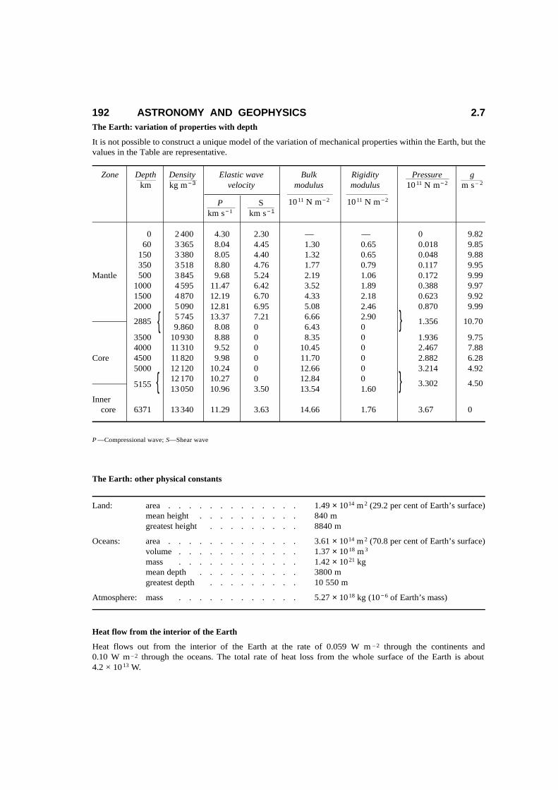
The Earth: variation of properties with depth

It is not possible to construct a unique model of the variation of mechanical properties within the Earth, but thevalues in the Table are representative.

The Earth: other physical constants

Heat flow from the interior of the Earth

Heat flows out from the interior of the Earth at the rate of 0.059 W m – 2 through the continents and 0.10 W m – 2 through the oceans. The total rate of heat loss from the whole surface of the Earth is about 4.2 × 10 13 W.


Land: area . . . . . . . . . . . . . 1.49 × 1014 m 2 (29.2 per cent of Earth’s surface)mean height . . . . . . . . . . 840 mgreatest height . . . . . . . . . 8840 m

Oceans: area . . . . . . . . . . . . . 3.61 × 1014 m 2 (70.8 per cent of Earth’s surface)volume . . . . . . . . . . . . 1.37 × 10 18 m 3

mass . . . . . . . . . . . . 1.42 × 10 21 kgmean depth . . . . . . . . . . 3800 mgreatest depth . . . . . . . . . 10 550 m

Atmosphere: mass . . . . . . . . . . . . 5.27 × 10 18 kg (10− 6 of Earth’s mass)

Zone Depth Density Elastic wave Bulk Rigidity Pressure gkm kg m− 3 velocity modulus modulus 10 11 N m− 2 m s – 2

P S 10 11 N m− 2 10 11 N m− 2

km s− 1 km s− 1

0 2 400 4.30 2.30 — — 0 9.8260 3 365 8.04 4.45 1.30 0.65 0.018 9.85

150 3 380 8.05 4.40 1.32 0.65 0.048 9.88350 3 518 8.80 4.76 1.77 0.79 0.117 9.95

Mantle 500 3 845 9.68 5.24 2.19 1.06 0.172 9.991000 4 595 11.47 6.42 3.52 1.89 0.388 9.971500 4 870 12.19 6.70 4.33 2.18 0.623 9.922000 5 090 12.81 6.95 5.08 2.46 0.870 9.99

2885 5 745 13.37 7.21 6.66 2.90 } 1.356 10.70{ 9.860 8.08 0 6.43 03500 10 930 8.88 0 8.35 0 1.936 9.754000 11 310 9.52 0 10.45 0 2.467 7.88

Core 4500 11 820 9.98 0 11.70 0 2.882 6.285000 12 120 10.24 0 12.66 0 3.214 4.92

5155 { 12 170 10.27 0 12.84 0 } 3.302 4.5013 050 10.96 3.50 13.54 1.60

Innercore 6371 13 340 11.29 3.63 14.66 1.76 3.67 0

P —Compressional wave; S—Shear wave

References

K. Bullen and B. A. Bolt (1985) An Introduction to the Theory of Seismology, Cambridge University Press,Cambridge.

Geodetic Reference System (1980), IUGG.J. G. Slater, C. Jaupart, and D. Galson (1970) Rev. Geophys. Space Phys. 18, 269–311. W. Torge (1991) Geodesy, 2nd edn, de Gruyter, Berlin, New York.

Sir Alan Cook

2.7.5 GravityThe gravity field of the Earth

The potential of the external gravity field of the Earth is usually expressed as a series of spherical harmonicterms:

where r = distance from the centre of the Eartha = Earth’s equatorial radius, θ = geocentric co-latitude,

M = mass of the Earth (see below) Pn(cos θ) = Legendre function of degree n

10 6J 2 = 1082.63 10 6J 3 = –2.5 10 6J 4 = –2.37The values of Jn are determined from the behaviour of artificial satellites about the Earth. (See section 2.7.4)The corresponding expression for the variation of the acceleration due to gravity over the surface of

the (spinning) Earth isg = ge(1 + β 1 sin 2 φ – β 2 sin2 2φ) – 3.088 × 10 – 6 H m s– 2

where φ is the geographical latitude, H is the height above sea level (in metres) and ge is the value of gravity at the equator.

The values recommended by the International Union of Geodesy and Geophysics arege = 9.780 327 m s – 2

β 1 = 0.005 302 4 β 2 = 0.000 005 8

The above formula gives the best simple method of calculating g at a place where it has not been meas-ured. It will almost always give results within 10 – 3 and usually within 5 × 10 – 4 m s – 2. The agreement withobservation is usually made worse by the application of a correction for the attraction of the land above sealevel.

The standard acceleration of gravity is defined as 9.80665 ms– 1 exactly.Absolute value of the acceleration due to gravity, g.Values of the acceleration due to gravity in terms of the fundamental units of length and time were, until recently, measured at very few sites and values elsewhere were found from measurements of differences. Inrecent years absolute apparatus using laser interferometer measurements of positions of falling reflectors hasbecome highly developed and easy to use. The constant term in the gravity above is now derived from a number of absolute measurements and it is no longer necessary to give an absolute value at one or two or three preferred sites.References

Geodetic Reference System (1980), IUGG.W. Torge, (1989) Gravimetry, de Gruyter, Berlin, New York.W. Torge, (1991), Geodesy, 2nd edn, de Gruyter, Berlin, New York.

Sir Alan Cook


GM ∝ aV = – [1 – Σ Jn ( )n

Pn (cosθ ) + terms depending on longitude]r n = 2 r

2.7.6 GeomagnetismThe Earth’s magnetic field corresponds approximately to that of a dipole situated at the centre of the Earth with its axis inclined at an angle of about 11° to the axis of rotation. There are, however, appreciable temporaland spatial departures from this simple model. According to presently accepted theories, the smooth geomagnetic or ‘normal’ field and its slow secular change are ascribed to fluid motions in the Earth’s electrically conducting core. The influence of magnetic constituents of crustal rocks superposes on the normalfield anomalies whose magnitude can, in extreme cases, be comparable to that of the normal field.

In addition, changes on the Sun and of its position relative to the Earth cause erratic and often rapid fluctuations in the magnetic field (magnetic storms) occasionally exceeding one-tenth of the normal field value,as well as smaller and more regular diurnal and seasonal variations.

The geomagnetic field at any point is usually defined by three of seven elements: five intensity components,H (parallel to the Earth’s surface), Z (vertically downwards), F or T (total, scalar), X (geographic north) and Y (geographic east); and two angles, D (declination or variation, D = arctan Y/X) and I (inclination or dip, I = arctan Z/H).

The main geomagnetic field, due to internal sources, at points on or above the Earth’s surface may be represented by the following series:

where a is the Earth’s mean radius, λ is east longitude, r is radial distance from the Earth’s centre and P mn(θ)

is an associated Legendre function of the colatitude or north polar distance, θ, of degree n and order m. The setof numerical coefficients (gm

n, hmn), usually expressed in units of nT, constitute a spherical harmonic model

of the geomagnetic field.The associated Legendre functions used in geomagnetism are of the Schmidt quasi-normalized form. They

are such that the mean square value of Pmn cos mλ or Pm

n sin mλ taken over a sphere is (2n + 1)–1 and may bederived from the relation:

where

c = cos θ

δm = 1 for m = 0; 2 for m >– 1

and

Pn(c) is the Legendre polynomial of degree n.

The International Geomagnetic Reference Field (IGRF) is a set of 21 spherical harmonic models: 20 describing the main geomagnetic field at epochs from 1900 to 1995, inclusive, five years apart and one for the (predicted) annual rate of secular variation for the interval 1995 to 2000. The main-field models extendto m = n = 10 (120 coefficients each) and the secular variation model is truncated at m = n = 8 (80 coefficients).Field component values for dates differing from the epochs of the main-field models are derived, for dates before1995, by linear interpolation and, for dates after 1995, by using the secular variation model to up-date the 1995main-field model. For further details see R. A. Langel (1992).

Figures 1 and 2 show contours of the declination and of the secular variation of the declination, respectively, at 1995 derived from the IGRF. A Fortran subroutine for synthesizing field component values from a spherical harmonic model is described by S. R. C. Malin and D. R. Barraclough (1981).

More detailed world magnetic charts are published by the Hydrographic Office of the Ministry of Defenceand are obtainable from Admiralty Chart Agents. The latest charts for all elements are for epoch 1995.


k n

X = Σ Σ (gmn cos mλ + hm

n sin mλ) (a/r)n + 2 dPmn (θ )

dθ,

n = 1 m = 0

k n

Y = Σ Σ (gmn sin mλ – hm

n cos mλ) (a/r)n + 2m cosec θPmn (θ ) ,

n = 1 m = 1

k n

Z = – Σ Σ (gmn cos mλ + hm

n sin mλ) (a/r)n + 2 (n + 1) Pmn (θ ) ,

n = 1 m = 0

δ m(n – m)!(1 – c2)m dm

Pmn (c) = ( )1/2

Pn(c)(n + m)! dc m


Con

tour

s of

mag

neti

c de

clin

atio

n at

199

5.0

from

the

6th

gen

erat

ion

IGR

F, in

deg

rees

.T

he c

onto

ur in

terv

al is

10°

. Pos

itive

(or

eas

t) d

eclin

atio

n is

indi

cate

d by

das

hed

lines

, zer

o an

d ne

gativ

e (o

r w

est)

dec

linat

ion

is in

dica

ted

by s

olid

line

s.


Con

tour

s of

sec

ular

vari

atio

n of

mag

netic

dec

linat

ion

for

the

inte

rval

199

0–19

95 f

rom

the

6th

gen

erar

atio

n IG

RF,

in

arcm

inut

es/y

ear.

The

co

ntou

r in

terv

al

is

2 ar

cmin

/yr.

Posi

tive

(or

east

) va

lues

ar

e in

dica

ted

by

dash

ed

lines

, ze

ro

and

nega

tive

(or

wes

t)

valu

es

are

indi

cate

d by

sol

id li

nes.

2.7 ASTRONOMY AND GEOPHYSICS 197Magnetic elements for London at different epochs

Values from 1850 onwards are for Greenwich. For 1580 the D observation was by Borough and the I value isNorman’s observation made about 1576.

Geomagnetic data 1990

The following table contains the mean values of D, H and Z observed during the year 1990 and their annualrates of change for a selection of permanent magnetic observatories.

Epoch Declination Inclination H /µT Z /µT

deg min deg min

1580 . . . . . . . . . . . . . . . 11 19 E 71 50 — —1665 . . . . . . . . . . . . . . . 0 0 — — —1673 . . . . . . . . . . . . . . . — 73 47 — —1719 . . . . . . . . . . . . . . . 11 30 W — — —1720 . . . . . . . . . . . . . . . — 75 14* — —1816 . . . . . . . . . . . . . . . 24 28 W* — — —1818 . . . . . . . . . . . . . . . — 70 35 — —1850 . . . . . . . . . . . . . . . 22 24 W 68 47 — —1875 . . . . . . . . . . . . . . . 19 21 W 67 42 17.97 43.831907 . . . . . . . . . . . . . . . 16 0 W 66 56 18.55* 43.571913 . . . . . . . . . . . . . . . 15 15 W 66 50† 18.53 43.321929 . . . . . . . . . . . . . . . 12 23 W 66 54 18.38 43.06†

1937 . . . . . . . . . . . . . . . 11 1 W 66 59 18.34† 43.171946 . . . . . . . . . . . . . . . 9 37 W 67 2* 18.39 43.371975 . . . . . . . . . . . . . . . 6 39 W 66 27 19.16 43.98

* Maximum. † Minimum.

Observatory Lat. Long. D Annual H Annual Z Annual change change change

deg deg deg nTnT

nTmin/yr nT/yr

Resolute Bay . +74.7 −94.9 −48.7 +79 1068 +30 58248 −30Bjørnøya . . +74.5 19.2 +4.3 +5 9027 −23 52875 −1Point Barrow . +71.3 −156.8 +25.0 −9 9504 −32 56270 −6Tromsø . . . +69.7 18.9 +1.5 +5 11146 −18 51624 +6College . . . +64.9 −147.8 +26.9 −11 12751 −24 55333 −6Lerwick (UK) +60.1 −1.2 −6.4 +8 14898 −4 48001 +17Magadan . . +60.1 151.0 −13.5 −2 17714 −20 52610 +24Moscow . . +55.5 37.3 +8.2 +1 17207 +13 48773 +5Eskdalemuir (UK) +55.3 −3.2 −6.9 +7 17314 +2 45950 +16Irkutsk . . . +52.2 104.4 −2.2 +2 19282 −26 56999 +13Hartland (UK) +51.0 −4.5 −6.2 +8 19395 +8 43896 +14Memambetsu . +43.9 144.2 −8.6 −2 26341 −18 41641 +42Coimbra . . +40.2 −8.4 −6.1 +6 25071 +10 36284 −12

(continued overleaf )

Geomagnetic data 1990 (contd)

References

R. A. Langel (1992) J. Geomagn. Geoelectr. 44, 679–707.S. R. C. Malin and D. R. Barraclough (1981) Computers and Geosciences 7, 401–405.

D.R.Barraclough

2.7.7 Cosmic raysThere is in nearby interstellar space a flux of particles—mostly protons and atomic nuclei—travelling at almostthe speed of light, having kinetic energies from below 108 eV to above 1020 eV. The flux reaching the solar system is virtually isotropic (to within 0.1% below 1014 eV) and unchanging, but the flux observed at the Earth varies somewhat because: (a) at energies below a few GeV, particles are affected by interplanetary magnetic fields, which cause intensity variations with an irregular 11-year period; and (b) the geomagnetic field deflects low-energy particles away from low-latitude regions. The particles incident at the top of theatmosphere are mainly protons and bare atomic nuclei: encounters with nuclei in the air generate secondary particles, and the less energetic particles are attenuated on traversing the atmosphere, so that near sea level the dominant particles are the penetrating secondary muons and the rapidly generated secondary electrons,positrons and photons.

Occasional bursts of particles originating in solar flares can reach a few GeV (usually having little effectat most sea level locations); there is also a variable anomalous component of nuclei below 0.1 GeV per nucleonoriginating in the solar system. These are not tabulated.


Observatory Lat. Long. D Annual H Annual Z Annual change change change

deg deg deg nTnT

nTmin/yr nT/yr

Fredericksburg +38.2 −77.4 −9.5 −6 20660 +17 50223 −105Kakioka . . +36.2 140.2 −6.8 −2 30136 −10 34953 +43Tucson . . . +32.2 −110.8 +11.8 −1 25342 −32 42505 −45Quetta . . . +30.2 67.0 +1.5 +1 32510 −5 33550 −15Honolulu . . +21.3 −158.0 +11.0 −4 27574 −13 22048 −26Alibag . . . +18.6 72.9 −0.5 +1 37982 −10 17982 +3San Juan . . +18.1 −66.2 −10.9 −8 27195 −6 29585 −146Guam . . . +13.6 144.9 +1.8 −1 35863 +3 7269 +20Bangui . . . +4.4 18.6 −2.0 +5 32028 −6 −9 294 −16Pamatai . . −17.6 −149.6 +11.3 0 30980 −34 −18926 −2Vassouras . . −22.4 –43.6 −20.3 −5 20332 −91 −12167 −89Hartebeesthoek −25.9 27.7 −16.0 −4 12879 −16 −26148 +74Gnangara . . −31.8 116.0 −3.1 +3 23195 −2 −53802 +13Hermanus . . −34.4 19.2 −23.4 −3 10932 −35 −24849 +92Canberra . . –35.3 149.4 +12.5 +1 23653 −6 −53663 +17Kerguelen . . −49.4 70.3 −53.0 −10 18603 −32 −44708 −4Macquarie Island −54.5 159.0 +29.7 +5 12577 −4 −63519 +32Mawson . . −67.6 62.9 −64.4 −8 18492 +14 −46015 +71

† Sign conventions: positive values of latitude are north; of longitude, and of D and its annual change are cast; and of Z and its annualchange are downwards.

Lat. Long.North magnetic dip-pole (1995) + 78.7º 104.8ºWSouth magnetic dip-pole (1995) – 64.6º 138.6ºE

Cosmic rays at the top of the atmosphere

The flux of particles per unit time, area and solid angle has a variation with energy of the general form

J (E ) dE ∝ E – γ dE,

where E is the particle’s kinetic energy (usually quoted in GeV). γ varies between 2.5 and 3.1 in different energyranges (see below). The integral flux, I(E), gives the flux of particles of kinetic energy >E: J = –dI/dE. The table below gives estimates of the particle flux at a time of minimum sunspot activity (when the flux is highest,as in 1965, 1977, 1987) and also (in italics) for a period of near maximum solar activity (low flux—though there is no well-defined absolute minimum). J and I are quoted for protons and I for the aggregate of all nuclear particles (including protons). Some compromises between inconsistent data mean that J and I are not always exactly consistent: errors of ~15% may be present in the fluxes for nuclei and protons: the uncertainties for electrons are much larger. To interpolate between quoted fluxes, a power law as quoted above is satisfactory: see also formulae given below. (The coverage is extended by empirical formulae givenlater.)

Fluxes observed (above atmosphere) where particles are not excluded by geomagnetic field

Differential flux J in m– 2 s – 1 sr – 1 GeV – 1, I in m– 2 s – 1 sr – 1.

The ‘electron’ flux includes positrons—about 30% of the total below 0.3 GeV, but only ~ 7% above 4 GeV. The photon flux above 0.1 GeV is 0.6 m– 2 s – 1 sr – 1 averaged over the sky, but 50% is from galactic latitudes<10°; about 20% is probably of extragalactic origin.

The more common nuclei heavier than protons have very similar spectra when expressed in terms of magnetic rigidity R = c . momentum/charge. (When v ~ c, R≈ (E + Mc 2) /eZ, Z being the nuclear charge number: thus a 100 GeV He nucleus has a rigidity of 52 GV.) Somewhat more convenient is to express the fluxes of cosmic ray nuclei in terms of kinetic energy-per-nucleon, U = E/A, where A is the atomic mass number. Over the range ~2 to 104 GeV/nucleon, the flux of some type of particle may be expressed to within~15% by

j(U) = C(U +V ) – γ particles m– 2 s – 1 sr – 1 (GeV/nucleon) – 1


E/GeV Jproton I proton I all nuclei Jelec I elec

0.1 1100 92 2900 1300 — — — ~8 — —0.2 1500 210 2800 1300 — 200 ~5 90 260.5 1600 420 2300 1200 2600 1400 70 10 60 241.0 1000 400 1700 1000 2000 1100 30 9 38 202.0 420 220 1000 700 1200 830 11 6 20 125.0 90 64 410 340 540 420 1.8 — 5 4

10 24 20 180 160 240 210 0.27 — 1.3 1.220 5 4.6 62 58 95 85 0.034 — 0.3 0.3

100 0.066 0.065 3.8 3.7 7.6 7.3 0.000 17 — — —1000 0.000 12 — 0.067 — 0.16 — — — — —5 × 10 6 — — — — 1.2 × 10 – 7 — — — —

10 9 — — — — 1.9 × 10 – 12 — — — —10 11 — — — — 0.8 km – 2 — — — —

century – 1 sr – 1

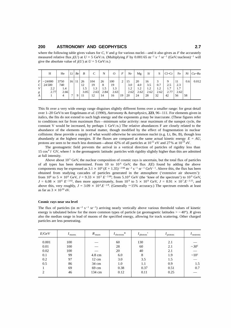
where the following table gives values for C, V and γ for various nuclei—and it also gives as F the accuratelymeasured relative flux j(U ) at U = 5 GeV/n. (Multiplying F by 0.001 65 m – 2 s – 1 sr – 1 (GeV/nucleon)– 1 willgive the absolute value of j(U ) at U = 5 GeV/n.)

This fit over a very wide energy range disguises slightly different forms over a smaller range: for great detailover 1–20 GeV/n see Engelmann et al. (1990), Astronomy & Astrophysics, 223, 96–111. For elements given initalics, the fits do not extend to such high energy and the exponents γ may be inaccurate. (These figures referto conditions not far from maximum flux—minimum solar activity: near maximum of the sunspot cycle, theconstant V would be increased, by perhaps 1 GeV/n.) The relative abundances F are closely related to the abundance of the elements in normal matter, though modified by the effect of fragmentation in nuclear collisions: these provide a supply of what would otherwise be uncommon nuclei (e.g. Li, Be, B), though lessabundantly at the highest energies. If the fluxes are compared at the same actual kinetic energy E = AU, protons are seen to be much less dominant—about 42% of all particles at 1012 eV and 27% at 10 14 eV.

The geomagnetic field prevents the arrival in a vertical direction of particles of rigidity less than 15 cos4 λ GV, where λ is the geomagnetic latitude: particles with rigidity slightly higher than this are admittedat full intensity.

Above about 10 5 GeV, the nuclear composition of cosmic rays is uncertain, but the total flux of particlesof all types has been determined. From 10 to 10 6 GeV, the flux J(E) found by adding the above components may be expressed as 3.1 × 104 (E + 1.35) – 2.68 m – 2 s – 1 sr – 1 GeV – 1. Above this, the flux has beenobtained from studying cascades of particles generated in the atmosphere (‘extensive air showers’): from 106 to 5 × 10 6 GeV, J = 9.33 × 10 3 E– 2.60; from 5.10 6 GeV (the ‘knee of the spectrum’) to 10 9 GeV, J = 6.08 × 10 6 E – 3.02, then more approximately, from 10 9 to 5 × 10 9 GeV, J = 8.91 × 10 7.E – 3.15, and above this, very roughly, J = 3.09 × 10 4.E – 2.8. (Generally ~15% accuracy.) The spectrum extends at least as far as 3 × 10 20 eV.

Cosmic rays near sea level

The flux of particles (in m – 2 s – 1 sr – 1) arriving nearly vertically above various threshold values of kinetic energy is tabulated below for the more common types of particle (at geomagnetic latitudes > ~ 40°). R givesalso the median range in lead of muons of the specified energy, allowing for track scattering. Other charged particles are less penetrating.


H He Li Be B C N O F Ne Mg Si S Cl−Cr Fe Ni Cu−Ru

F ~24000 3750 16 11 26 104 26 100 2 15 20 16 3 9 11 0.6 0.012C 24 500 740 12 19 8 19 3.0 4.0 3.5 0.7 2.5 2.3V 2.2 1.4 1.5 1.3 1.5 1.3 1.2 1.2 1.2 1.2 1.7 1.7γ 2.77 2.66 3.05 2.63 2.84 2.63 2.62 2.62 2.62 2.62 2.77 2.62A 1 4 7 9 11 12 14 16 19 20 24 28 32 42 56 58

E/GeV I muons R muon I electrons* I photons† I protons I neutrons

0.001 100 — 60 130 2.1 —0.01 100 — 28 60 2.1 ~ 30‡

0.02 100 — 20 40 2.1 —0.1 99 4.8 cm 6.0 8 1.9 ~10‡

0.2 97 12 cm 3.0 3.5 1.5 —0.5 86 34 cm 1.0 1.1 0.9 1.51 69 69 cm 0.38 0.37 0.51 0.72 46 134 cm 0.12 0.11 0.25 —

Above 100 GeV, pions will have fluxes comparable to nucleons: they are less important at lower energies.Fluxes are averaged over the 11-year cycle. The total muon flux will vary about 3% either way: above

1 GeV the variation is slight. The muon fluxes are the best determined—a few percent at low E (20% say at100 GeV); the proton flux is uncertain to tens of percent above a few GeV.

Away from the vertical direction, the muon flux per unit solid angle varies with zenith angle θ, approximately as I ∝ cos n θ, with n = 2.15, out to 80° (these refer to the total flux including all energies: muons of tens of GeV vary little with zenith angle). For the protons and neutrons, however, at least above tens of MeV, n ~ 8. About 20% of the electrons striking the ground will be distributed like nucleons, the restlike muons. With a zenith-angle variation of this form, the flux passing through unit horizontal surface, integrated over a hemisphere of angles, is 2π/(n + 2) times the vertical flux per unit solid angle, as tabulatedabove. Thus a thin, horizontal plane detector will record a flux per m2 per second of about 150 muons and, if its wall has 1 MeV electron stopping power, 70 electrons, and 1 proton.

Nuclear interactions of cosmic rays in the atmosphere generate about 6 × 10 4 neutrons s– 1 per m2 of theEarth at 45° latitude, of which 4 × 104 m–2s–1 are absorbed by nitrogen to generate 14C when solar activity is low: the long-term all-Earth average would be about 60% of this. 0.05 –0.13 (or 0.2) neutrons s – 1 are generated per kg of air (or Pb) near sea level, at latitudes >40° at times of low solar activity.

Showers. Primary cosmic rays above ~ 10 12 eV generate extensive showers of secondary particles in the atmosphere and above ~10 14 eV these penetrate to sea level. At this level, such a shower contains about 1charged particle per 10 GeV of primary energy (at 1014 eV, or 1 per 3 GeV at 1017 eV, 1 per 1.6 GeV at 10 20 eV): 5% of the particles are within 3 m of the centre, 50% are within 40 m and 90% within ~250 m. Most of the particles are electrons and positrons; a few percent are penetrating muons. A burst of > 100 particles m – 2 over a few m 2 due to a shower in the air would be seen about once per hour near sea level under a very thin cover (mass can add local showers), and > 650 m – 2 once per day, the rate of showers doubling per 100 mb reduction in atmospheric overlay.

Variation with latitude. The number of vertical muons above 0.2 GeV is typically about 13% lower at theequator than at high geomagnetic latitudes; above 50° the flux does not change much. The component generating neutrons by nuclear interactions (largely the neutrons below 1 GeV)—long used to monitor cosmicray variations—falls by about 24% in going from latitude 55° to the equator.

Variations with time. During the course of the 11-year sunspot cycle, the flux of neutron-generating particlesnear sea level varies by about 20%, being highest in years of low solar activity (e.g. 1954, 1965, less well-defined in 1977, 1987), though the variation is far from smooth. Flux minima occurred in 1947, 1958,1969, 1982. The muon flux varies much less.


E/GeV I muons R muon I electrons* I photons† I protons I neutrons

5 20 3.1 m 0.02 0.02 0.077 —10 8.6 5.8 m — — 0.025 ~ Ip20 3.0 — — — 0.008 —50 0.58 — — — 0.001 6 —

100 0.14 — — — 4.3 × 10 − 4 —200 0.030 — — — 1.1 × 10 − 4 —500 3.2 × 10 − 3 — — — 2 × 10 − 5 —1000 5 × 10 − 4 — — — — —

* 40 – 50% are positrons, above 0.1 GeV (but only ~5% at 1 MeV).† Theoretical values, as measurements are inadequate.‡ Uncertain angular distribution makes vertical flux uncertain.

Cosmic rays as background radiation. Near sea level the dose equivalent rate of cosmic rays, describing theirmedical (whole body) effect, is about 0.31 mSv per year (somewhat less at latitudes < 30°), but this might beonly a third or less of the total natural dose. The dose increases by about 3% per 100 m up in the lower atmosphere. (Above the atmosphere the dose due to low-energy nuclei is very much larger.)

Cosmic radiation is more penetrating than radioactive emissions. The particles penetrating more than 5 cm of lead are mostly muons (only above 0.7 GeV does an electron produce more than 0.5 particle under such a shield), so the particle flux penetrating a thickness x of absorber normally may be judged from the table above—shielding materials of ligher elements are more effective than lead (for a given mass per unit area) by about a factor 1.4, but lead is much more effective in cutting out electrons and photons.

Cosmic rays at other levels

Some muons have extraordinary penetrating power. The following table gives their flux in the vertical direction(in m– 2 s – 1 sr – 1 ) under specified masses h of ‘standard rock’ (having effective Z2 /A = 5.5). The mass is givenin tonnes m – 2, equivalent in mass to metres of water, and, roughly, to feet of rock. The actual depth of waterwhich is estimated to have the same stopping power is also given, though measurements at great depths of water are not yet available.

At great depths, the chemical composition of the rock (Z2/A) can have a large effect. The flux at angle θ to the vertical, under rock, may be estimated quite well from the formula

H being the mass overlay measured along the slant direction from the top of the atmosphere: H = h rock, slant +(10 sec θ). For standard rock, k = 7.1 × 10 – 4, but if the rock has Z2/A = 6.37, as at the Kolar Gold Fields, where many of the observations were made, k = 8 × 10 – 4. The formula fits the observations to about 15% for small angles and for depths of more than a few metres, and probably for θ up to 45°.

Above ground level, the absorption length, in which the intensity increases by a factor e, is roughly as follows, for the lower half of the atmosphere:

Nucleons above a few GeV, 110 g cm– 2; total muon flux, 550 g cm – 2;total electronic flux, 180 g cm– 2; nuclear disintegrations 165 g cm– 2.

The rate of nuclear disintegration reaches a peak near the 100 millibar level, several hundred times the sea-levelrate (depending on latitude). At this level, though, large increases due to solar flares occasionally occur, lastingfor a few hours.

A.M.Hillas

2.7.8 The atmosphereVariation of pressure, density and temperature with altitude

Values given in the table are based on the standard atmosphere of the International Civil Aviation Organization (ICAO). They are representative of average atmospheric conditions in temperate latitudes.


h (standard rock) 50 100 200 500 1000 2000 4000 7000 10 000Water depth (km) 0.043 0.087 0.175 0.450 0.92 2.0 4.3 8.2 12.5Flux (m − 2 s − 1 sr − 1) 7.7 2.5 0.65 0.081 0.013 1.4 × 10 − 3 7.0 × 10 − 5 1.9 × 10 − 6 1 × 10 − 7

1.7 × 106 secθI(h,θ ) = H – 1.53 e – kH m – 2 s – 1 sr – 1

H + 390 secθ

Reference

Manual of ICAO Standard Atmosphere (1964) International Civil Aviation Organization Doc. 7488/2, ICAO, Montreal, Canada.

K.W.T.Elliott

Pressure, mean molecular weight and temperature in the upper atmosphere


Altitude Pressure Density Temperature Altitude Pressure Density Temperaturem kPa kg m−3 °C m kPa kg m−3 °C

−250 104.4 1.25 17 6 000 47.2 0.66 −240 101.3 1.22 15 7 000 41.1 0.59 −30

250 98.4 1.20 13 8 000 35.6 0.53 −37500 95.5 1.17 12 9 000 30.7 0.47 −44750 92.6 1.14 10 10 000 26.4 0.41 −50

1000 89.9 1.11 8 12 000 19.3 0.31 −561500 84.6 1.06 5 14 000 14.1 0.23 −562000 79.5 1.00 2 16 000 10.3 0.17 −562500 74.7 0.96 −1 18 000 7.5 0.12 −563000 70.1 0.91 −4 20 000 5.5 0.088 −563500 65.8 0.86 −8 22 000 4.0 0.064 −544000 61.6 0.82 −11 24 000 2.9 0.046 −524500 57.7 0.78 −14 26 000 2.2 0.034 −505000 54.0 0.74 −18 28 000 1.6 0.025 −48

30 000 1.2 0.018 −46

Altitude /km Mean molecular Pressure /Pa Temp./Kweight

30 . . . . . . . . . . . . . . . . 28.97 1.20 × 10 3 230.140 . . . . . . . . . . . . . . . . 28.97 2.94 × 10 2 250.550 . . . . . . . . . . . . . . . . 28.97 8.10 × 10 1 271.060 . . . . . . . . . . . . . . . . 28.97 2.19 × 10 1 243.370 . . . . . . . . . . . . . . . . 28.97 5.12 × 10 0 216.680 . . . . . . . . . . . . . . . . 28.96 9.75 × 10 – 1 186.090 . . . . . . . . . . . . . . . . 28.94 1.63 × 10 – 1 186.0

100 . . . . . . . . . . . . . . . . 28.30 3.10 × 10 – 2 208.1120 . . . . . . . . . . . . . . . . 27.01 2.73 × 10 – 3 355.7150 . . . . . . . . . . . . . . . . 25.17 4.70 × 10 – 4 652

200Night . . . . . . . . . . . . . 22.7 9.5 × 10 – 5 890{ Day . . . . . . . . . . . . . 23.0 1.2 × 10 – 4 1100

300Night . . . . . . . . . . . . . 18.6 8.9 × 10 – 6 980{ Day . . . . . . . . . . . . . 19.7 1.8 × 10 – 5 1360

500Night . . . . . . . . . . . . . 15.0 2.8 × 10 – 7 1000{ Day . . . . . . . . . . . . . 16.3 1.3 × 10 – 6 1420

800Night . . . . . . . . . . . . . 6.5 1.1 × 10 – 8 1000{ Day . . . . . . . . . . . . . 12.1 6.6 × 10 – 8 1430

The above values are a mean over all conditions. Considerable variation occurs with latitude, season and(above 100 km) with solar activity. Above 100 km the composition of the atmosphere changes due to dissociation and diffusive separation, the main constituents in addition to N2 and O 2 being atomic oxygen and helium.

Reference

COSPAR International Reference Atmosphere, (1965) North Holland Publishing Co.Sir John Houghton

2.7.9 Physical properties of sea waterThe properties of sea water are a function of temperature, salinity (i.e. total dissolved solids in g kg – 1) and pressure. For the sources of the data see M. Hill (ed.), The Sea, vol. 1, chap. 1 and vol. 4, pt. 1, chap. 18 (Wiley) and Cox et al., Deep Sea Res., 1970, 17, 679. For chemical composition see section 3.1.3.

Density ρ of sea water at atmospheric pressure

Density ρ of sea water at 0 °C and salinity 35 g kg – 1

Mechanical and thermal properties of sea water at salinity 35 g kg – 1 and atmospheric pressure (unless otherwisestated)


Temperature Salinity (g kg – 1)

°C20 25 30 35 40

(ρ /kg m– 3 – 1000)*

0 . . . . . . . . . . . 16.04 20.06 24.08 28.10 32.145 . . . . . . . . . . . 15.84 19.78 23.73 27.68 31.64

10 . . . . . . . . . . . 15.31 19.18 23.07 26.96 30.8615 . . . . . . . . . . . 14.48 18.30 22.13 25.97 29.8220 . . . . . . . . . . . 13.39 17.17 20.96 24.75 28.5625 . . . . . . . . . . . 12.07 15.82 19.57 23.34 27.12

* In oceanographical work these data are always expressed in terms of 1000(S – 1) where S is the density relative to water at 4 °C. Values for this can be obtained by adding 0.03 to the values in the table.

Pressure /MPa 0 20 40 60 80 100

(ρ /kg m– 3 – 1000) 28.10 37.44 46.37 54.92 63.12 71.02

Property 0 °C 20 °C

Dynamic viscosity . . . . . . . . . . . 1.88 × 10 – 3 Pa s 1.08 × 10 – 3 Pa sKinematic viscosity, v . . . . . . . . . . 1.83 × 10 – 6 m 2 s – 1 1.05 × 10 – 6 m 2 s – 1

Thermal conductivity . . . . . . . . . . 0.563 W m – 1 K – 1 0.596 W m – 1 K – 1

Thermal diffusivity, κ . . . . . . . . . . 1.37 × 10 – 7 m 2 s – 1 1.46 × 10 – 7 m 2 s – 1

Prandtl number, v/κ . . . . . . . . . . . 13.4 7.2

Mechanical and thermal properties of sea water at salinity 35 g kg – 1 and atmospheric pressure (unless otherwisestated) (contd)

Electrical conductivity γ of sea water at atmospheric pressure

At a depth of 4000 m the bottom water (about 0 °C, salinity 35 g kg – 1) has a conductivity 6% greater than thesurface water. The mean conductivity of the oceans (excluding the shallow seas) is 3.27 S m– 1.

Sir Edward Bullard


Temperature Salinity / (g kg – 1)

°C20 25 30 35 40

γ / (S m– 1 )

0 . . . . . . . . . . . 1.745 2.137 2.523 2.906 3.2855 . . . . . . . . . . . 2.015 2.466 2.909 3.346 3.778

10 . . . . . . . . . . . 2.300 2.811 3.313 3.808 4.29715 . . . . . . . . . . . 2.595 3.170 3.735 4.290 4.83720 . . . . . . . . . . . 2.901 3.542 4.171 4.788 5.39725 . . . . . . . . . . . 3.217 3.926 4.621 5.302 5.974

Property 0 °C 20 °C

Specific hear capacity, Cp . . . . . . . . . 3985 J kg – 1 K – 1 3993 J kg – 1 K – 1

Thermal expansion coefficient . . . . . . .Pressure = 0.1 MN m – 2 . . . . . . . . 52 × 10 – 6 K – 1 250 × 10 – 6 K – 1

Pressure = 100 MN m – 2 . . . . . . . . 244 × 10 – 6 K – 1 325 × 10 – 6 K – 1

Ratio of specific hear capacities, Cp /Cv . . . . 1.000 4 1.010 6Velocity of sound* . . . . . . . . . . . 1449 m s – 1 1522 m s – 1

Compressibility . . . . . . . . . . . . 4.65 × 10 – 10 Pa – 1 4.28 × 10 – 10 Pa – 1

Freezing point . . . . . . . . . . . . – 1.910 °CBoiling point . . . . . . . . . . . . . 100.56 °C

* See also section 2.4.1.

2.7.10 The geological timescaleIn assessing the relative age of rock formations, superposition of uninterrupted and undisturbed strata establishes a stratigraphic sequence (i.e. older below younger), while the thickness of deposition is a guide tothe time period of sedimentary accretion. In palaeontology, the presence of fossils from the Cambrian periodonwards promotes a correlation between strata in different areas. Geological Periods, collected into palaeontological Era, have been named after the districts in which the rock horizons were classically identified.

A variety of geochronological techniques are available. The most recent past is indicated from dendrochronology (annular growth rings in very old trees), or the examination of a sequence of glacial meltwater varves (upper Pleistocene lacustrine deposits); both methods are related to changes in terrestrial climate and solar excursions. For anthropological specimens less than 1.5 million years old, fluorine dating(Oakley, 1980) may provide relative estimates of contemporaneous age of associated specimens, at least one of which has been dated by independent stratigraphic, cultural or absolute means. Their inter-relation is inferred from chemical measurement of fluorine /phosphate ratios (Glover and Phillips, 1965) of apatite mineral in bone, teeth, antlers, etc. from contiguous horizons.

Absolute age may be computed from the decay of various radioisotopes which occur in specific relationships ‘starting’ from some geomorphological or biological event. Radiocarbon dating relies on a livingorganism exchanging carbon dioxide at an equilibrium level of 14C/ 12C until it dies; the level of 14C then decays according to its 5730 year half-life. Dates are reliable to 5% or better but this scale is only useful forevents in the last 70 000 years. For earlier events, e.g. in the Tertiary Era, the measurement of 40K/ 40A ratios in micaceous and volcanic rocks has been notable in assessing the antiquity of fossil remains of very earlyhominids and anthrapoids found in East Africa. Dating of older (e.g. Palaeozoic) rock formations relies ondetermining the ratios of longer lived isotopes, e.g. 87Rb/87Sr or various uranium/lead ratios. Estimates of the age of the earth’s crust have been derived from ratios of 206Pb and 207Pb to (nonradiogenic) 204Pb.

(See section 4.6.2 for an exposition of the uranium and thorium radioactive disintegration series.)Harland and colleagues (1990) developed a chronostratic scale of rock sequences (with data through 1988)

which assigns ages with standardised stratigraphic reference points. In the following table, the geological periods are mostly given classic (West) European stage names but some broadly equivalent East European and Asian strata (marked ‘*’) have been included. For more detailed reference there is a useful wall chart byhis co-author Smith (1990) based on their book but with some minor revisions.

In the table, the age point for the base bed of most systems has been abstracted from data in Harland et al. (1990).

References

M. J. Glover and G. F. Phillips (1965) J. Appl. Chem., 15, 570−576.W. B. Harland et al., (1990) A geological time scale 1989, Cambridge University Press.K. P. Oakley (1980) Relative dating of the fossil hominids of Europe, Bull. Br. Mus. Nat. Hist. 34(1).A. G. Smith (1990) Wall chart: a geological time scale 1989, Cambridge University Press.

G.F.Phillips


The geological timescale 1989

Age points are expressed in million years; uncertainties are generally around 5 in the last digit


ERA, Period and Epoch Bed Base Duration ERA, Period and Epoch Bed Base Duration

QUATERNARY PRIMARY = PALAEOZOICHOLOCENE – post-Glacial 0.01 0.01

upper PERMIAN Zechstein 256.1 11.0 45PLEISTOCENE 1.64 1.63 lower PERMIAN *Kungurian 259.7 3.6

Rotliegendes *Artinskian 268.8 9.1TERTIARY = CENOZOIC *Sakmarian 281.5 12.7PLIOCENE Asselian 290.0 8.5

upper Piacenzian 3.4 1.8 3.6lower Zanclian 5.2 1.8 upper CARBONIFEROUS = Silesian

NA2 Stephanian 295.1 5.1 33MIOCENE Messinian 6.7 1.5 18 Westphalian 311.3 16.2

Tortonian 10.4 3.7 Namurian 322.8 11.5Serravallian 14.2 3.8 lower CARBONIFEROUS = DinantianLanghian 16.3 2.1 NA1 Viséan 349.5 26.7 40Burdigalian 21.5 5.2 Tournaisian 362.5 13.0Aquitanian 23.3 1.8

upper DEVONIAN Famennian 367.0 4.5 46OLIGOCENE Chattian 29.3 6.0 12 D3 Frasnian 377.4 10.4

Rupelian 35.4 6.1 middleDEVONIAN Givetian 380.8 3.4

EOCENE Priabonian 38.6 3.2 21 D2 Eifelian 386.0 5.2Bartonian 42.1 3.5 lower DEVONIAN Emsian 390.4 4.4Lurtetian 50.0 7.9 D1 Siegenian/Pragian 396.3 5.9Ypresian 56.5 6.5 Gedinnian/ 408.5 12.2

LochkovianPALAEOCENE Thanetian 60.5 4.0 10

Montian + Danian 65.0 4.5 SILURIAN Ludlow 424.0 15.5 30Wenlock 430.4 6.4Valentian/ 439.0 8.6Llandovery

SECONDARY = MESOZOICupper CRETACEOUS K2 upper

Maastrichtian 74.0 9.0 32 ORDOVICIAN Ashgill 443.1 4.1 71Campanian 83.0 9.0 Bala Caradoc 463.9 20.8

Senonian { Santonian 86.6 3.6 middleConiacian 88.5 1.9 ORDOVICIAN Llandeilo 468.6 4.7Turonian 90.4 1.9 Dyfed Llanvirn 476.2 7.6Cenomanian 97.0 6.6 lower

ORDOVICIAN Arenig 493.0 16.8lower CRETACEOUS K1 Canadian Tremadoc 510.0 17.0

Albian 112.0 15.0 49Aptian 124.5 12.5 upper CAMBRIAN Merioneth 517.2 7.2 60

Barremian 131.8 7.3 middle

Necomian 145.6 13.8 CAMBRIAN St Davids 536.0 18.8lower CAMBRIAN Lenian/Comley 553.7 17.7

upper JURASSIC J3 Caerfai Atdabanian 560 6.3Purbeckian 62 Tommotian 570 10

Tithonian { Portlandian} 152.1 6.5Malm Kimmeridgian 154.7 2.6 PROTEROZOICOxfordian 157.1 2.4 SINIAN Neoproterozoic 230middle JURASSIC Callovian 161.3 4.2 Pt3 Poundian 580 10J2 Bathonian 166.1 4.8 Wonokan 590 10Dogger Bajocian 173.5 7.4 Vendian { Mortensnes 600 10Aslenian 178.0 4.5 Smâlfjord 610 10lower JURASSIC Toarcian 187.0 9.0 Sturtian ca 800 190J1 Pliensbachian 194.5 7.5Lias Sinemurian 203.5 9.0 RIPHEAN/HELIKIAN Mesoproterozoic 850

Hettangian 208.0 4.5 Pt2 Karatau 1050 250Yurmatin 1350 300

upper TRIASSIC Rhaetic 209.5 1.5 37 Burzyan 1650 300TR3 Keuper Norian 223.4 13.9

*Karnian 235.0 11.6 APHEBIAN Palaeoproterozoic 750middle TRIASSIC *Ladinian 239.5 4.5 Pt1 Animikean 2200 550TR2 Muschelkalk *Anisian 241.1 1.6 Huronian 2400 200lower TRIASSIC Scythian

AZOIC = ARCHEAN ca 4500 ca 2100TR1 Bunter *Olenekian ca 245 ca 4crust formation without organic life

2.7 astronomy and geophysics - national physical · pdf file2.7 astronomy and geophysics ......

Documents