26 machine learning unsupervised fuzzy c-means
TRANSCRIPT

Machine Learning for Data MiningFuzzy Clustering
Andres Mendez-Vazquez
July 27, 2015
1 / 39

Images/cinvestav-1.jpg
Outline
1 Fuzzy ClusteringHistoryFuzzy C-Means ClusteringUsing the Lagrange MultipliersThe Final Algorithm!!!Pros and Cons of FCM
2 What can we do? Possibilistic ClusteringIntroductionCost FunctionExplanation
2 / 39

Images/cinvestav-1.jpg
Outline
1 Fuzzy ClusteringHistoryFuzzy C-Means ClusteringUsing the Lagrange MultipliersThe Final Algorithm!!!Pros and Cons of FCM
2 What can we do? Possibilistic ClusteringIntroductionCost FunctionExplanation
3 / 39

Images/cinvestav-1.jpg
Some of the Fuzzy Clustering Models
Fuzzy Clustering ModelBezdek, 1981
Possibilistic Clustering ModelKrishnapuram - Keller, 1993
Fuzzy Possibilistic Clustering ModelN. Pal - K. Pal - Bezdek, 1997
4 / 39

Images/cinvestav-1.jpg
Some of the Fuzzy Clustering Models
Fuzzy Clustering ModelBezdek, 1981
Possibilistic Clustering ModelKrishnapuram - Keller, 1993
Fuzzy Possibilistic Clustering ModelN. Pal - K. Pal - Bezdek, 1997
4 / 39

Images/cinvestav-1.jpg
Some of the Fuzzy Clustering Models
Fuzzy Clustering ModelBezdek, 1981
Possibilistic Clustering ModelKrishnapuram - Keller, 1993
Fuzzy Possibilistic Clustering ModelN. Pal - K. Pal - Bezdek, 1997
4 / 39

Images/cinvestav-1.jpg
Outline
1 Fuzzy ClusteringHistoryFuzzy C-Means ClusteringUsing the Lagrange MultipliersThe Final Algorithm!!!Pros and Cons of FCM
2 What can we do? Possibilistic ClusteringIntroductionCost FunctionExplanation
5 / 39

Images/cinvestav-1.jpg
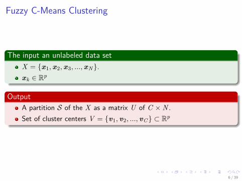
Fuzzy C-Means Clustering
The input an unlabeled data setX = {x1,x2,x3, ...,xN}.xk ∈ Rp
OutputA partition S of the X as a matrix U of C ×N .Set of cluster centers V = {v1, v2, ..., vC} ⊂ Rp
6 / 39
Images/cinvestav-1.jpg
Fuzzy C-Means Clustering
The input an unlabeled data setX = {x1,x2,x3, ...,xN}.xk ∈ Rp
OutputA partition S of the X as a matrix U of C ×N .Set of cluster centers V = {v1, v2, ..., vC} ⊂ Rp
6 / 39

Images/cinvestav-1.jpg
What we want
Creation of the Cost FunctionFirst:
We can use a distance defined as:
‖xk − vi‖ =√
(xk − vi)T (xk − vi) (1)
The euclidean distance from a point k to a centroid i.NOTE other distances based in Mahalonobis can be taken inconsideration.
7 / 39

Images/cinvestav-1.jpg
What we want
Creation of the Cost FunctionFirst:
We can use a distance defined as:
‖xk − vi‖ =√
(xk − vi)T (xk − vi) (1)
The euclidean distance from a point k to a centroid i.NOTE other distances based in Mahalonobis can be taken inconsideration.
7 / 39

Images/cinvestav-1.jpg
What we want
Creation of the Cost FunctionFirst:
We can use a distance defined as:
‖xk − vi‖ =√
(xk − vi)T (xk − vi) (1)
The euclidean distance from a point k to a centroid i.NOTE other distances based in Mahalonobis can be taken inconsideration.
7 / 39

Images/cinvestav-1.jpg
Do you remember the cost function for K -means?
Finding a partition S that minimizes the following function
minS
N∑k=1
∑k:xk∈Ci
‖xk − vi‖2 (2)
Where vi = 1Ni
∑xk∈Ci
xk
We can rewrite the previous equation as
minS
N∑k=1
C∑i=1
I (xk ∈ Ci) ‖xk − vi‖2 (3)
8 / 39

Images/cinvestav-1.jpg
Do you remember the cost function for K -means?
Finding a partition S that minimizes the following function
minS
N∑k=1
∑k:xk∈Ci
‖xk − vi‖2 (2)
Where vi = 1Ni
∑xk∈Ci
xk
We can rewrite the previous equation as
minS
N∑k=1
C∑i=1
I (xk ∈ Ci) ‖xk − vi‖2 (3)
8 / 39

Images/cinvestav-1.jpg
In addition
Did you notice that the membership is always one or zero?
minS
N∑k=1
C∑i=1
Membership︷ ︸︸ ︷I (xk ∈ Ci) ‖xk − vi‖2 (4)
9 / 39

Images/cinvestav-1.jpg
Thus, we can rethink the membership using something“Fuzzy”
What if we modify the cost function to something like this
minS
N∑k=1
C∑i=1
Membership︷ ︸︸ ︷Fuzzy Value ‖xk − vi‖2 (5)
This means that we think that each cluster Ci is “Fuzzy”We can assume a fuzzy set for the cluster Ci with memebership function:
Ai : Rp → [0, 1] (6)
Such that we can tune it by using a power i.e. decreasing it by a m power.
10 / 39

Images/cinvestav-1.jpg
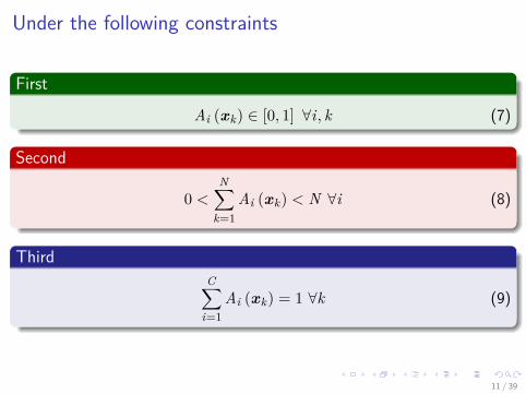
Under the following constraints
First
Ai (xk) ∈ [0, 1] ∀i, k (7)
Second
0 <N∑
k=1Ai (xk) < N ∀i (8)
ThirdC∑
i=1Ai (xk) = 1 ∀k (9)
11 / 39

Images/cinvestav-1.jpg
Under the following constraints
First
Ai (xk) ∈ [0, 1] ∀i, k (7)
Second
0 <N∑
k=1Ai (xk) < N ∀i (8)
ThirdC∑
i=1Ai (xk) = 1 ∀k (9)
11 / 39
Images/cinvestav-1.jpg
Under the following constraints
First
Ai (xk) ∈ [0, 1] ∀i, k (7)
Second
0 <N∑
k=1Ai (xk) < N ∀i (8)
ThirdC∑
i=1Ai (xk) = 1 ∀k (9)
11 / 39

Images/cinvestav-1.jpg
Final Cost Function
Properties
Jm (S) =N∑
k=1
C∑i=1
[Ai (xk)]m ‖xk − vi‖2 (10)
Under the constraintsAi (xk) ∈ [0, 1], for 1 ≤ k ≤ N and 1 ≤ i ≤ C .∑C
i=1 Ai (xk) = 1, for 1 ≤ k ≤ N .0 <
∑Nk=1 Ai (xk) < n, for 1 ≤ i ≤ C .
m > 1.
12 / 39

Images/cinvestav-1.jpg
Final Cost Function
Properties
Jm (S) =N∑
k=1
C∑i=1
[Ai (xk)]m ‖xk − vi‖2 (10)
Under the constraintsAi (xk) ∈ [0, 1], for 1 ≤ k ≤ N and 1 ≤ i ≤ C .∑C
i=1 Ai (xk) = 1, for 1 ≤ k ≤ N .0 <
∑Nk=1 Ai (xk) < n, for 1 ≤ i ≤ C .
m > 1.
12 / 39

Images/cinvestav-1.jpg
Final Cost Function
Properties
Jm (S) =N∑
k=1
C∑i=1
[Ai (xk)]m ‖xk − vi‖2 (10)
Under the constraintsAi (xk) ∈ [0, 1], for 1 ≤ k ≤ N and 1 ≤ i ≤ C .∑C
i=1 Ai (xk) = 1, for 1 ≤ k ≤ N .0 <
∑Nk=1 Ai (xk) < n, for 1 ≤ i ≤ C .
m > 1.
12 / 39

Images/cinvestav-1.jpg
Final Cost Function
Properties
Jm (S) =N∑
k=1
C∑i=1
[Ai (xk)]m ‖xk − vi‖2 (10)
Under the constraintsAi (xk) ∈ [0, 1], for 1 ≤ k ≤ N and 1 ≤ i ≤ C .∑C
i=1 Ai (xk) = 1, for 1 ≤ k ≤ N .0 <
∑Nk=1 Ai (xk) < n, for 1 ≤ i ≤ C .
m > 1.
12 / 39

Images/cinvestav-1.jpg
Final Cost Function
Properties
Jm (S) =N∑
k=1
C∑i=1
[Ai (xk)]m ‖xk − vi‖2 (10)
Under the constraintsAi (xk) ∈ [0, 1], for 1 ≤ k ≤ N and 1 ≤ i ≤ C .∑C
i=1 Ai (xk) = 1, for 1 ≤ k ≤ N .0 <
∑Nk=1 Ai (xk) < n, for 1 ≤ i ≤ C .
m > 1.
12 / 39

Images/cinvestav-1.jpg
Outline
1 Fuzzy ClusteringHistoryFuzzy C-Means ClusteringUsing the Lagrange MultipliersThe Final Algorithm!!!Pros and Cons of FCM
2 What can we do? Possibilistic ClusteringIntroductionCost FunctionExplanation
13 / 39

Images/cinvestav-1.jpg
Using the Lagrange Multipliers
New cost function
J̄m (S) =N∑
k=1
C∑i=1
[Ai (xk)]m ‖xk − vi‖2 −N∑
k=1λk
[ C∑i=1
Ai (xk)− 1]
(11)
Derive with respect to Ai (xk)∂J̄m (S)∂Ai (xk) = mAi (xk)m−1 ‖xk − vi‖2 − λk = 0 (12)
Thus
Ai (xk) =[
λk
m ‖xk − vi‖2
] 1m−1
(13)
14 / 39

Images/cinvestav-1.jpg
Using the Lagrange Multipliers
New cost function
J̄m (S) =N∑
k=1
C∑i=1
[Ai (xk)]m ‖xk − vi‖2 −N∑
k=1λk
[ C∑i=1
Ai (xk)− 1]
(11)
Derive with respect to Ai (xk)∂J̄m (S)∂Ai (xk) = mAi (xk)m−1 ‖xk − vi‖2 − λk = 0 (12)
Thus
Ai (xk) =[
λk
m ‖xk − vi‖2
] 1m−1
(13)
14 / 39

Images/cinvestav-1.jpg
Using the Lagrange Multipliers
New cost function
J̄m (S) =N∑
k=1
C∑i=1
[Ai (xk)]m ‖xk − vi‖2 −N∑
k=1λk
[ C∑i=1
Ai (xk)− 1]
(11)
Derive with respect to Ai (xk)∂J̄m (S)∂Ai (xk) = mAi (xk)m−1 ‖xk − vi‖2 − λk = 0 (12)
Thus
Ai (xk) =[
λk
m ‖xk − vi‖2
] 1m−1
(13)
14 / 39

Images/cinvestav-1.jpg
Using the Lagrange MultipliersSum over all i’s
C∑i=1
Ai (xk) = λ1
m−1k
m1
m−1 ‖xk − vi‖2
m−1(14)
Thus
λk = m[∑Ci=1
1‖xk−vi‖
2m−1
]m−1 (15)
Plug Back on equation 12 using j instead of im[∑C
j=11
‖xk−vj‖2
m−1
]m−1 = mAi (xk)m−1 ‖xk − vi‖2 (16)
15 / 39

Images/cinvestav-1.jpg
Using the Lagrange MultipliersSum over all i’s
C∑i=1
Ai (xk) = λ1
m−1k
m1
m−1 ‖xk − vi‖2
m−1(14)
Thus
λk = m[∑Ci=1
1‖xk−vi‖
2m−1
]m−1 (15)
Plug Back on equation 12 using j instead of im[∑C
j=11
‖xk−vj‖2
m−1
]m−1 = mAi (xk)m−1 ‖xk − vi‖2 (16)
15 / 39

Images/cinvestav-1.jpg
Using the Lagrange MultipliersSum over all i’s
C∑i=1
Ai (xk) = λ1
m−1k
m1
m−1 ‖xk − vi‖2
m−1(14)
Thus
λk = m[∑Ci=1
1‖xk−vi‖
2m−1
]m−1 (15)
Plug Back on equation 12 using j instead of im[∑C
j=11
‖xk−vj‖2
m−1
]m−1 = mAi (xk)m−1 ‖xk − vi‖2 (16)
15 / 39

Images/cinvestav-1.jpg
Finally
We have that
Ai (xk) = 1[∑Cj=1
{‖xk−vi‖2
‖xk−vj‖2
} 1m−1
] (17)
In a similar way we have
vi =∑N
k=1 Ai (xk)m xk∑Nk=1 Ai (xk)m (18)
16 / 39

Images/cinvestav-1.jpg
Finally
We have that
Ai (xk) = 1[∑Cj=1
{‖xk−vi‖2
‖xk−vj‖2
} 1m−1
] (17)
In a similar way we have
vi =∑N
k=1 Ai (xk)m xk∑Nk=1 Ai (xk)m (18)
16 / 39

Images/cinvestav-1.jpg
Outline
1 Fuzzy ClusteringHistoryFuzzy C-Means ClusteringUsing the Lagrange MultipliersThe Final Algorithm!!!Pros and Cons of FCM
2 What can we do? Possibilistic ClusteringIntroductionCost FunctionExplanation
17 / 39

Images/cinvestav-1.jpg
Final AlgorithmFuzzy c-means
1 Let t = 0. Select an initial fuzzy pseudo-partition.
2 Calculate the initial C cluster centers using, v(t)i =
∑Nk=1 A(t)
i (xk)mxk∑Nk=1 A(t)
i (xk)m .
3 Update for each xk the membership function by
I Case I:∥∥∥xk − v(t)
i
∥∥∥2> 0 for all i ∈ {1, 2, ...,C} then
A(t+1)i (xk) = 1[∑C
j=1
{‖xk −v(t)
i ‖2
‖xk −v(t)j ‖
2
} 1m−1]
I Case II:∥∥∥xk − v(t)
i
∥∥∥2= 0 for some i ∈ I ⊆ {1, 2, ...,C} then define
A(t+1)i (xk) by any nonnegative number such that
∑i∈I Ai (xk) = 1
and A(t+1)i (xk) = 0 for i /∈ I .
4 If∣∣∣S(t+1) − S(t)
∣∣∣ = maxi,k
∣∣∣A(t+1)i (xk)−A(t)
i (xk)∣∣∣ ≤ ε stop; otherwise
increase t and go to step 2.18 / 39

Images/cinvestav-1.jpg
Final Output
The Matrix UThe elements of U are Uik = Ai (xk).
The centroidsV = {v1, v2, ..., vC}
19 / 39

Images/cinvestav-1.jpg
Final Output
The Matrix UThe elements of U are Uik = Ai (xk).
The centroidsV = {v1, v2, ..., vC}
19 / 39

Images/cinvestav-1.jpg
Outline
1 Fuzzy ClusteringHistoryFuzzy C-Means ClusteringUsing the Lagrange MultipliersThe Final Algorithm!!!Pros and Cons of FCM
2 What can we do? Possibilistic ClusteringIntroductionCost FunctionExplanation
20 / 39

Images/cinvestav-1.jpg
Pros and Cons of Fuzzy C-Means
AdvantagesUnsupervisedAlways converges
DisadvantagesLong computational timeSensitivity to the initial guess (speed, local minima)Sensitivity to noise
I One expects low (or even no) membership degree for outliers (noisypoints)
21 / 39

Images/cinvestav-1.jpg
Pros and Cons of Fuzzy C-Means
AdvantagesUnsupervisedAlways converges
DisadvantagesLong computational timeSensitivity to the initial guess (speed, local minima)Sensitivity to noise
I One expects low (or even no) membership degree for outliers (noisypoints)
21 / 39

Images/cinvestav-1.jpg
Pros and Cons of Fuzzy C-Means
AdvantagesUnsupervisedAlways converges
DisadvantagesLong computational timeSensitivity to the initial guess (speed, local minima)Sensitivity to noise
I One expects low (or even no) membership degree for outliers (noisypoints)
21 / 39

Images/cinvestav-1.jpg
Pros and Cons of Fuzzy C-Means
AdvantagesUnsupervisedAlways converges
DisadvantagesLong computational timeSensitivity to the initial guess (speed, local minima)Sensitivity to noise
I One expects low (or even no) membership degree for outliers (noisypoints)
21 / 39

Images/cinvestav-1.jpg
Pros and Cons of Fuzzy C-Means
AdvantagesUnsupervisedAlways converges
DisadvantagesLong computational timeSensitivity to the initial guess (speed, local minima)Sensitivity to noise
I One expects low (or even no) membership degree for outliers (noisypoints)
21 / 39

Images/cinvestav-1.jpg
Pros and Cons of Fuzzy C-Means
AdvantagesUnsupervisedAlways converges
DisadvantagesLong computational timeSensitivity to the initial guess (speed, local minima)Sensitivity to noise
I One expects low (or even no) membership degree for outliers (noisypoints)
21 / 39

Images/cinvestav-1.jpg
Outliers, Disadvantage of FCMAfter running without outliers
0
1
22 / 39

Images/cinvestav-1.jpg
Outliers, Disadvantage of FCMNow add an outlier
0
1
23 / 39

Images/cinvestav-1.jpg
Outline
1 Fuzzy ClusteringHistoryFuzzy C-Means ClusteringUsing the Lagrange MultipliersThe Final Algorithm!!!Pros and Cons of FCM
2 What can we do? Possibilistic ClusteringIntroductionCost FunctionExplanation
24 / 39

Images/cinvestav-1.jpg
Krinshapuram and Keller
Following ZadehThey took in consideration that each class prototype as defining an elasticconstraint.
What?Giving the ti (xk) as degree of compatibility of sample xk with cluster Ci .
We do the followingIf we consider the Ci as fuzzy sets over the set of samplesX = {x1,x2, ...,xN}
25 / 39

Images/cinvestav-1.jpg
Here is the Catch!!!
We should not use the old membershipC∑
i=1Ai (xk) = 1 (19)
BecauseThis is quite probabilistic... which is not what we want!!!
ThusWe only ask for membership, now using the possibilistic notation of ti (xk)(This is known as typicality value), to be in the interval [0, 1].
26 / 39

Images/cinvestav-1.jpg
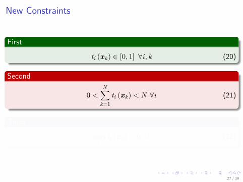
New Constraints
First
ti (xk) ∈ [0, 1] ∀i, k (20)
Second
0 <N∑
k=1ti (xk) < N ∀i (21)
Third
maxi
ti (xk) > 0 ∀k (22)
27 / 39
Images/cinvestav-1.jpg
New Constraints
First
ti (xk) ∈ [0, 1] ∀i, k (20)
Second
0 <N∑
k=1ti (xk) < N ∀i (21)
Third
maxi
ti (xk) > 0 ∀k (22)
27 / 39

Images/cinvestav-1.jpg
New Constraints
First
ti (xk) ∈ [0, 1] ∀i, k (20)
Second
0 <N∑
k=1ti (xk) < N ∀i (21)
Third
maxi
ti (xk) > 0 ∀k (22)
27 / 39

Images/cinvestav-1.jpg
Outline
1 Fuzzy ClusteringHistoryFuzzy C-Means ClusteringUsing the Lagrange MultipliersThe Final Algorithm!!!Pros and Cons of FCM
2 What can we do? Possibilistic ClusteringIntroductionCost FunctionExplanation
28 / 39

Images/cinvestav-1.jpg
We have the following cost function
Cost FunctionN∑
k=1
C∑i=1
[ti (xk)]m ‖xk − vi‖2 (23)
ProblemUnconstrained optimization of first term will lead to the trivial solutionti (xk) = 0 for all i, k.
Thus, we can introduce the following constraint
ti (xk)→ 1 (24)
Roughly it means to make the typicality values as large as possible.
29 / 39

Images/cinvestav-1.jpg
We can try to control this tendency
By putting all them together inN∑
k=1(1− ti (xk))m (25)
With m to control the tendency of ti (xk)→ 1
We can also run this tendency over all the cluster using a suitablewi > 0 per cluster
C∑i=1
wi
N∑k=1
(1− ti (xk))m (26)
30 / 39

Images/cinvestav-1.jpg
We can try to control this tendency
By putting all them together inN∑
k=1(1− ti (xk))m (25)
With m to control the tendency of ti (xk)→ 1
We can also run this tendency over all the cluster using a suitablewi > 0 per cluster
C∑i=1
wi
N∑k=1
(1− ti (xk))m (26)
30 / 39

Images/cinvestav-1.jpg
Possibilistic C-Mean Clustering (PCM)
The final Cost Function
Jm (S) =N∑
k=1
C∑i=1
[ti (xk)]m ‖xk − vi‖2 +C∑
i=1wi
N∑k=1
(1− ti (xk))m (27)
Whereti (xk) are typicality values.wi are cluster weights
31 / 39

Images/cinvestav-1.jpg
Possibilistic C-Mean Clustering (PCM)
The final Cost Function
Jm (S) =N∑
k=1
C∑i=1
[ti (xk)]m ‖xk − vi‖2 +C∑
i=1wi
N∑k=1
(1− ti (xk))m (27)
Whereti (xk) are typicality values.wi are cluster weights
31 / 39

Images/cinvestav-1.jpg
Outline
1 Fuzzy ClusteringHistoryFuzzy C-Means ClusteringUsing the Lagrange MultipliersThe Final Algorithm!!!Pros and Cons of FCM
2 What can we do? Possibilistic ClusteringIntroductionCost FunctionExplanation
32 / 39

Images/cinvestav-1.jpg
Explanation
First TermN∑
k=1
C∑i=1
[ti (xk)]m ‖xk − vi‖2 (28)
It demands that the distance from feature vector to prototypes be as smallas possible!!!
Second Termc∑
i=1wi
n∑k=1
(1− ti (xk))m (29)
It forces the typicality values ti (xk) to be as large as possible.
33 / 39

Images/cinvestav-1.jpg
Explanation
First TermN∑
k=1
C∑i=1
[ti (xk)]m ‖xk − vi‖2 (28)
It demands that the distance from feature vector to prototypes be as smallas possible!!!
Second Termc∑
i=1wi
n∑k=1
(1− ti (xk))m (29)
It forces the typicality values ti (xk) to be as large as possible.
33 / 39

Images/cinvestav-1.jpg
Explanation
First TermN∑
k=1
C∑i=1
[ti (xk)]m ‖xk − vi‖2 (28)
It demands that the distance from feature vector to prototypes be as smallas possible!!!
Second Termc∑
i=1wi
n∑k=1
(1− ti (xk))m (29)
It forces the typicality values ti (xk) to be as large as possible.
33 / 39

Images/cinvestav-1.jpg
Explanation
First TermN∑
k=1
C∑i=1
[ti (xk)]m ‖xk − vi‖2 (28)
It demands that the distance from feature vector to prototypes be as smallas possible!!!
Second Termc∑
i=1wi
n∑k=1
(1− ti (xk))m (29)
It forces the typicality values ti (xk) to be as large as possible.
33 / 39

Images/cinvestav-1.jpg
Final Updating Equations
Typicality Values
ti (xk) = 1
1 +(‖xk−vi‖2
wi
) 1m−1
, ∀i, k (30)
Cluster Centers
vi =∑N
k=1 ti (xk)m xk∑nk=1 ti (xk)m (31)
34 / 39

Images/cinvestav-1.jpg
Final Updating Equations
Typicality Values
ti (xk) = 1
1 +(‖xk−vi‖2
wi
) 1m−1
, ∀i, k (30)
Cluster Centers
vi =∑N
k=1 ti (xk)m xk∑nk=1 ti (xk)m (31)
34 / 39

Images/cinvestav-1.jpg
Final Updating Equations
Weights
wi = M∑N
k=1 [ti (xk)]m ‖xk − vi‖2∑nk=1 [ti (xk)]m , (32)
with M > 0.
35 / 39

Images/cinvestav-1.jpg
Possibilistic can deal with outliersAfter running without outliers
0
1
36 / 39

Images/cinvestav-1.jpg
Possibilistic can deal with outliersNow add an outlier
0
1
37 / 39

Images/cinvestav-1.jpg
Pros and Cons of Fuzzy C-Means
AdvantagesClustering noisy data samples.
DisadvantagesVery sensitive to good initialization.
In Between!!!Coincident clusters may result.
Because the columns and rows of the typicality matrix areindependent of each other.This could be advantageous (start with a large value of C and getless distinct clusters)
38 / 39

Images/cinvestav-1.jpg
Nevertheless
There are more advanced clustering methods based on thepossibilistic and fuzzy ideaPal, N.R.; Pal, K.; Keller, J.M.; Bezdek, J.C., "A Possibilistic Fuzzyc-Means Clustering Algorithm," Fuzzy Systems, IEEE Transactions on ,vol.13, no.4, pp.517,530, Aug. 2005.
39 / 39