25 the impact of some macroeconomic determinants - faaeza atiq

Vol. V, No. II (Spring 2020) Global Social Sciences Review (GSSR) p- ISSN: 2520-0348 URL: http://dx.doi.org/10.31703/gssr.2020(V-II).25 e-ISSN: 2616-793X DOI: 10.31703/gssr.2020(V-II).25 ISSN-L: 2520-0348 Pages: 260‒ 272

Citation: Atiq, F., Uddin, M., & Khan, I. H. (2020). The Impact of Key Macroeconomic Determinants on Pakistan’s Economy. Global Social Sciences Review, V(II), 260-272. https://doi.org/10.31703/gssr.2020(V-II).25

Faaeza Atiq* Mudassir Uddin† Irfan Hussain Khan‡

The Impact of Key Macroeconomic Determinants on Pakistan’s Economy

‘This paper intended to analyze key Macroeconomic factor’s effect on Pakistan’s economic development. The annual time-series data has been taken from 1980 to 2018 on External Debts,

Foreign Direct investment. Consumer Price Index and Term of Trade. Variables stationarity is analyzed by ADF and Ng-Perron tests; afterwards, JJ test and Granger Causality test are used for Long-run (LR) & Short-run(SR) associations between variables, respectively. Also, Residuals Diagnostic Test used for checking residuals assumptions and CUSUM and CUSUMSQ are used for checking parameter constancy. The result shows significantly negative and positive long-run effects of External Debts and Foreign Direct Investment (FDI) respectively on the economic growth of Pakistan. Albeit, Consumer Price Index (CPI), Term of Trade (TOT) and, FDI significantly Granger cause economic growth in the short-run. Research suggests that economic policies devised in such a way that deteriorates External Debts and attract foreign investments and strengthen the economic growth of Pakistan in the long-term.

Key Words: Johansen’s Co-Integration Method; Granger Causality; External Debt; Economic Growth

Introduction Foreign debt has always been a notable factor for developing nations because it plays a vital role in the economic development of any country if used with proper management and policies. Pakistan has an immense amount of natural resources, good geographical and weather conditions as well as talented minds and young human capital in its region which leads to any country to its apex despite all these factors Pakistan developing indicators, economic and socio-economic conditions remains poor. Nowadays Pakistan’s sovereignty is threatening by its poor economic condition due to which Pakistan must take foreign debts which turns into a basic issue for policymakers that there is a need to re-examine the components and determinants of economic growth. Since 1980 Pakistan’s economic edifice is descending, total debt (internal and external) has reached its peak in June 2018 which is 28.879 trillion rupees and exceeded to Rs. 35.094 trillion till the end of March 2019 alternatively per capita debt in Pakistan reached to approximately two hundred thousand rupees which are a 350% increased as compared to 2008; Inflation has marked up to 15%. Moreover, Pakistan’s debt servicing is increasing sharply along with aggravated debt to GDP ratio, which has touched to 71.69% in 2018. Pakistan is dependent on borrowing from external sources rather than focusing on our resources such as foreign direct investment which creates the most detrimental impact on the current economic crisis that has brought national development halt and low tax collection and inefficiency within the tax system raises the budget deficit. The above short financial glimpse propelled 40% of Pakistan’s population below the poverty line and creating extreme economic frustration and social unrest. Under the present global economic meltdown to find the alternate and independent economic strategy which must be sustainable in the long-term. This paper is intended to identify and analyze economic growth factor which can help the policymaker in devising an economic strategy.

However, the changing conditions of politics and economics, it seems necessary to carry out more investigation by using current data and econometrics methods. A review of the literature summarizes as under. These studies have revealed numerous factors that were held responsible for

* University of Karachi, Sindh, Pakistan. Email: [email protected] † Professor, Department of Statistics, University of Karachi, Sindh, Pakistan. ‡ Department of Economics, Government College University Faisalabad, Punjab, Pakistan.

Abstract


Vol. V, No. II (Spring 2020) 261

predicting Economic patterns (Eichengreen & Portes, 1986) revealed that foreign indebtedness might cause export instability and trade openness in emergent nations.

Ferraro & Rosser (1994) also tried to find causal factors for high external debt ratio in underdeveloped countries, and they deduced that rise in interest rate, fluctuation in oil prices 1973 and 1979, decrease in terms of trade and poverty were the main cause for the accumulation of debts. By utilizing the panel data approach, the underlying cause of foreign indebtedness of emerging countries is income stability, debt servicing, poverty, exchange difference gap & capital-output during the 1980s toward the 1990s. This study called for attention toward those factors that are responsible for indebtedness and drowsy economic development which includes income instability, high dependence on foreign loans to pay import bills and, debt service instalments. (Tiruneh, 2004)

Zafar & Butt (2008) by applying the econometric technique on the data from 1972 to 2007 to analyze the consequences of trade openness on the accumulation of external debt of Pakistan. It has been identified that trade openness was the main factor to increase foreign debt in Pakistan, which hamper economic progress. Identified beneficial factors that accentuate economic growth include credit to the private sector, FDI & the inflow of remittances on economic development of Pakistan by utilizing the Autoregressive Distributed Lag (ARDL) approach and log-linear model. However, it turned out that trade openness and inflation inversely effect on the development of the country (Shahbaz et al., 2008). As along both Japan and Korea for 1971-2006 and 1996-2003 respectively. By using the Johansen Cointegration method, it concluded that the Term of Trade (TOT) has an inverse effect on Economic development (Wong, 2010). FDI and CPI that either affects the Gross Domestic products of SAARC countries or not. The investigation reasoned that the general model in these nations built up a positive association with Foreign Direct Investment, while GDP was inversely influenced by CPI. The information of the SAARC nations extended from the year 2001 to 2010 (Abbaset al.l, 2011). Moreover, external debts have more negative effects on economic development than domestic debts and slow down the progress of any country because more amount of income produced by individuals was given as debt servicing which cause a consistent budget deficit issue of the country. Literature Review Sulaiman & Azeez (2012) explained the case study of Nigeria, where data extracted from 1970 to 2010. This study used Johansen’s cointegration technique and showed that external debt has positively affected economic development.

Saqib et al. (2013) suggested that FDI in developing countries like Pakistan plays a negative role not just only FDI, but debts, inflation and, trade have a jointly negative influence on the economy of Pakistan, but domestic investment in this regards beneficial for the country. Therefore, dependency on FDI should remain limited.

Havi et al. (2013) explained that Johansen’s cointegration method through the neo-classical growth model identified that physical capital, FDI, labour force, CPI, government spending, military rule were notable components helped to contribute in real GDP per capita of this country.

Abdalla & Abdelbaki (2014) utilized the JJ and VECM to identify the core factors of economic progress, independently for all Gulf Cooperation Council (GCC) individuals. The outcomes reveal that FDI and gross capital formation were the essentials of economic development in Bahrain. While for Kuwait, Saudi Arabia and Qatar exports and gross capital formation were the core factors respectively, and in the UAE, two other factors were Foreign Direct Investment and exports. There was no cointegrating vector among the variables in Oman.

Kalumbu & Sheefeni (2014) examined data from 1980 to 2018 to discover the relation between TOT and the economic development of Namibia. The cointegration technique was being used, and it is found that TOT harms economic growth.

Siddique et al. (2015) examines data of 40 countries to discover the relation between economic development and debts and also used population, capital formation and, trade as other significant factors and found that capital formation has a positive influence on the long and short-term but debts may harm in the LR as well as SR while the economic growth influenced positively by the increase in population.

Chaudhry et al. (2017) studied over the sample of 25 region-wise emerging countries by using

Faaeza Atiq, Mudassir Uddin and Irfan Hussain Khan

262 Global Social Science Review (GSSR)

Johansen Fisher Panel Co-Integration Test. This study concluded that to grow the economy of the nation, two factors were essential, FDI and, External Debts. Further, this study found that government expenditure, labour and, gross domestic savings also positively affect economic growth, while gross capital formation has a declining effect on economic development.

Gudaro et al. (2010) found that FDI influenced positively, while CPI has a significant adverse influence on economic development. In addition to FDI positively affect the economy of emerging countries as cited the study of Agrawal et al. (2015)

Akram (2017) analyzed the data of Sri Lanka from 1975 to 2014 by using the ARDL method. The conclusion of this study showed that foreign debts negatively influenced the economic development, but foreign debts(as a percentage of GDP) had helped to process the economic development in the time of civil war in Sri Lanka while debt servicing also inversely affect the GDP per capita and investment. As well as domestic debts positively associated with per capita GDP.

Jebran et al. (2018) explained the study conducted on Pakistan’s Economic growth by taking a sample from 1980 to 2013. To deduce the result, the autoregressive distributed lag model was used. Result induced that TOT had a negative influence on economic development. In the wake of the current situation, whereas as found that there are various components inferred in economic development. External debt accumulation is one of the factors which have threatening behaviour for developing countries like Pakistan. Because due to high indebtedness, one cannot make the monetary policies for their benefit, especially when Pakistan’s political and monetary policies have changed rapidly for almost three decades. There is a need to recognize the components responsible to hinder the economic growth. Given the outcomes, the examined features will help to strategize the alternatives that may get accommodating for the legislature to make improved conditions for economic growth. Methodology To conduct this study, the cointegration technique is being used to find the correlation among some time series variables. First, the model VAR (Vector Autoregressive) has been utilized before the model can be picked; the stationarity of the data must be checked. To check the stationarity of variables time series plot, unit root tests, and correlogram of ACF can be utilized. The subsequent stage is to test the cointegration to examine the LR association among the variables. At the point when the data gets stationary at order one, and there is a cointegration relationship, at that point, the model VAR which will be utilized is VECM. Fundamentally, two techniques of cointegration that have reliably been utilized. First was EG(Engle-Grangers) Two-Step Estimation Method & second was Johansen’s ML(Maximum Likelihood).

Along these lines, to dissect the relationship among at least two non-stationary time variables, we have two techniques which are referenced previously. In this paper, the Johansen’s Method was being used for analyzing five macro-economic determinants as we need the capacity to inspect them in a multivariate structure, taking into consideration the conceivable disclosure of more than one cointegrating vector, which the EG Two-step Estimation Method can’t achieve. Right now, JJ better option to be used as per the requirement of this study, because this method can examine two or more variables and treated all the variables as endogenous (Brooks,.2008). Unit Root Test In this study, two tests have been used to verify the stationarity and the order of the series, ADF Test and Ng-Perron test. Many researchers criticized the low power test of ADF due to which we used the Ng-Perron test as well because it is viewed as a better test for a limited sample size. ADF To carry out this study, we will test each variable independently by unit root test to guarantee their non-stationarity at the level, and then they become stationary at I(1). Tsay (2005) proposed to confirm the presence of a unit root in an autoregressive AR(p) procedure; one may test the following hypothesis



𝐻! : β = 1 vs. 𝐻" : β < 1 using the regression

𝑦# = 𝑐# + 𝛽𝑦#$% +∑ 𝜙&'$%&(% ∆𝑦#$& + Ԑ# Eq 1. 1

where 𝑐# is a deterministic function of the time index t and ∆𝑦) = 𝑦) − 𝑦)$%is the differenced series of 𝑦#. 𝑐# can be zero or a constant or 𝑐# = ω0 + ω1t.

The equation for the ADF_Test is given below:

𝐴𝐷𝐹_𝑇𝑒𝑠𝑡 = +,$%-#.(+,)

Eq 1. 2

where 𝛽4 is the least-squares estimate of β, which is known as the ADF method unit-root test. After the first differencing equation one can be written as:

∆𝑦# =𝑐# + 𝛽1𝑦#$% +∑ 𝜙&'$%&(% ∆𝑦#$& + Ԑ# Eq 1. 3

where 𝛽1 = β – 1 which can be tested with the hypothesis 𝐻!: 𝛽1 = 0 against𝐻": 𝛽1 < 0. It is necessary to determine the optimal lag length for each model. Therefore, to maximize the

log-likelihood function of the model one must choose the model with the lowest SBIC (Schwartz Bayesian Information Criterion) and for accuracy Cross-check it by using the AIC (Akaike Information Criterion).

Ng et al. (2011) argued that ADF_Test is not that decisive in limited sample sizes. This test tends to reject when the null hypothesis is true and accept when it is false. Therefore Ng & Perron (2001) developed four test statistics by using the GLS method detrended procedure to solve the difficulties regarding power distortion and meagre sample size, which is associated with the ADF test. Johansen’s Cointegration Method Johansen’s Cointegration method is utilized when we need to see the correlation among at least two non-stationary time series variables, and they must be stationary at I(1) independently so their combination will likewise be I(1). Nonetheless, it is conceivable that two non-stationary variables, i.e. I(1) can be cointegrated if their linear combination would be stationary, which is I(0).

If we combine variables with varying order of difference, then the combination of integration will be the order of the higher one, i.e., if

𝑌&,#~𝐼(𝑑&) Eq 1. 4 for i=1,2,3…. k

𝑋# =∑ 𝛽&𝑌&,#3&(% Eq 1. 5

Let then 𝑋#~𝐼(max 𝑑&) Eq 1. 6

It shows a steady-state or long-run relationship among variables which might be a consequence of economic behaviours and patterns.

The method uses in this study is Johansen & Juselius (1990) this procedure depends on the maximum likely hood method. For applying this method first, we should need to select the ideal lag length for the Gaussian error term, which is no autocorrelation and heteroskedasticity and normally distributed. Their approach decides the numbers of cointegrating vectors in non-stationary time series. VAR which can be composed as:

𝑦# = 𝛼 + ∑ Π3𝑦#$343$% + 𝜖# Eq 1. 7

Where 𝑦#is a matrix of five variables having dimension gx1 and they should be integrated at I(1), 𝛼 is a vector of constant with dimensions gx1and 𝜖# is a vector of an error term with zero mean and constant variance having dimension gx1.

After the first difference, it turns into VECM which can be written as:

∆𝑦# = 𝛼 +∑ Γ3∆𝑦#$34$%3$% +Π𝑦#$% + 𝜖# Eq 1. 8

Where 𝑦# and 𝜖# are the vectors of five variables and the white noise error term, respectively. K shows lag length. Π is a long-term coefficient matrix which is also known as impact matrix with the



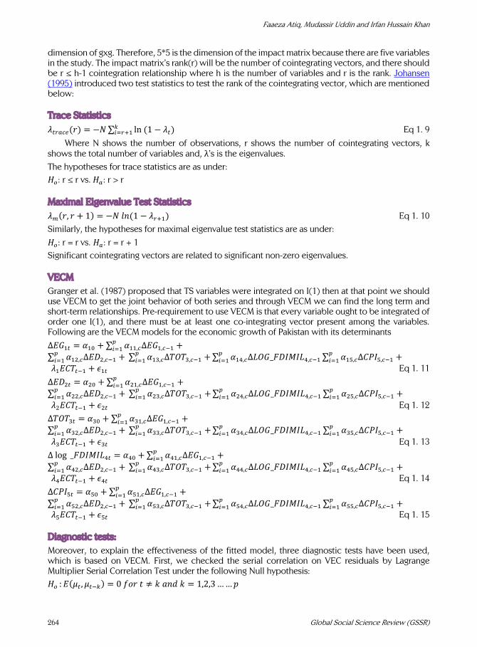
dimension of gxg. Therefore, 5*5 is the dimension of the impact matrix because there are five variables in the study. The impact matrix’s rank(r) will be the number of cointegrating vectors, and there should be r ≤ h-1 cointegration relationship where h is the number of variables and r is the rank. Johansen (1995) introduced two test statistics to test the rank of the cointegrating vector, which are mentioned below: Trace Statistics

𝜆#5"16(𝑟) = −𝑁∑ ln(1 − 𝜆#)3&(57% Eq 1. 9

Where N shows the number of observations, r shows the number of cointegrating vectors, k shows the total number of variables and, λ’s is the eigenvalues.

The hypotheses for trace statistics are as under:

𝐻!: r ≤ r vs.𝐻": r > r Maximal Eigenvalue Test Statistics 𝜆4(𝑟, 𝑟 + 1) = −𝑁𝑙𝑛(1 − 𝜆57%) Eq 1. 10

Similarly, the hypotheses for maximal eigenvalue test statistics are as under:

𝐻!: r = r vs. 𝐻": r = r + 1

Significant cointegrating vectors are related to significant non-zero eigenvalues. VECM Granger et al. (1987) proposed that TS variables were integrated on I(1) then at that point we should use VECM to get the joint behavior of both series and through VECM we can find the long term and short-term relationships. Pre-requirement to use VECM is that every variable ought to be integrated of order one I(1), and there must be at least one co-integrating vector present among the variables. Following are the VECM models for the economic growth of Pakistan with its determinants

∆𝐸𝐺%# = 𝛼%8 +∑ 𝛼%%,1∆𝐸𝐺%,1$%'&(% +

∑ 𝛼%9,1∆𝐸𝐷9,1$% +'&(% ∑ 𝛼%:,1∆𝑇𝑂𝑇:,1$% +

'&(% ∑ 𝛼%;,1∆𝐿𝑂𝐺_𝐹𝐷𝐼𝑀𝐼𝐿;,1$%∑ 𝛼%<,1∆𝐶𝑃𝐼<,1$% +

'&(%

'&(%

𝜆%𝐸𝐶𝑇#$% + 𝜖%# Eq 1. 11

∆𝐸𝐷9# = 𝛼98 +∑ 𝛼9%,1∆𝐸𝐺%,1$%'&(% +

∑ 𝛼99,1∆𝐸𝐷9,1$% +'&(% ∑ 𝛼9:,1∆𝑇𝑂𝑇:,1$% +

'&(% ∑ 𝛼9;,1∆𝐿𝑂𝐺_𝐹𝐷𝐼𝑀𝐼𝐿;,1$%∑ 𝛼9<,1∆𝐶𝑃𝐼<,1$% +

'&(%

'&(%

𝜆9𝐸𝐶𝑇#$% + 𝜖9# Eq 1. 12

∆𝑇𝑂𝑇:# = 𝛼:8 + ∑ 𝛼:%,1∆𝐸𝐺%,1$%'&(% +

∑ 𝛼:9,1∆𝐸𝐷9,1$% +'&(% ∑ 𝛼::,1∆𝑇𝑂𝑇:,1$% +

'&(% ∑ 𝛼:;,1∆𝐿𝑂𝐺_𝐹𝐷𝐼𝑀𝐼𝐿;,1$%∑ 𝛼:<,1∆𝐶𝑃𝐼<,1$% +

'&(%

'&(%

𝜆:𝐸𝐶𝑇#$% + 𝜖:# Eq 1. 13

∆log _𝐹𝐷𝐼𝑀𝐼𝐿;# = 𝛼;8 +∑ 𝛼;%,1∆𝐸𝐺%,1$%'&(% +

∑ 𝛼;9,1∆𝐸𝐷9,1$% +'&(% ∑ 𝛼;:,1∆𝑇𝑂𝑇:,1$% +

'&(% ∑ 𝛼;;,1∆𝐿𝑂𝐺_𝐹𝐷𝐼𝑀𝐼𝐿;,1$%∑ 𝛼;<,1∆𝐶𝑃𝐼<,1$% +

'&(%

'&(%

𝜆;𝐸𝐶𝑇#$% + 𝜖;# Eq 1. 14

∆𝐶𝑃𝐼<# = 𝛼<8 +∑ 𝛼<%,1∆𝐸𝐺%,1$%'&(% +

∑ 𝛼<9,1∆𝐸𝐷9,1$% +'&(% ∑ 𝛼<:,1∆𝑇𝑂𝑇:,1$% +

'&(% ∑ 𝛼<;,1∆𝐿𝑂𝐺_𝐹𝐷𝐼𝑀𝐼𝐿;,1$%∑ 𝛼<<,1∆𝐶𝑃𝐼<,1$% +

'&(%

'&(%

𝜆<𝐸𝐶𝑇#$% + 𝜖<# Eq 1. 15 Diagnostic tests: Moreover, to explain the effectiveness of the fitted model, three diagnostic tests have been used, which is based on VECM. First, we checked the serial correlation on VEC residuals by Lagrange Multiplier Serial Correlation Test under the following Null hypothesis:

𝐻!: 𝐸(𝜇#, 𝜇#$3) = 0𝑓𝑜𝑟𝑡 ≠ 𝑘𝑎𝑛𝑑𝑘 = 1,2,3……𝑝



Second, we checked the normality of the VEC residuals by Jarque_Bera test under the following Null Hypothesis:

𝐻!: 𝑅𝑒𝑠𝑖𝑑𝑢𝑎𝑙𝑠𝑎𝑟𝑒𝑛𝑜𝑟𝑚𝑎𝑙𝑙𝑦𝑑𝑖𝑠𝑡𝑟𝑖𝑏𝑢𝑡𝑒𝑑

Third, we checked Heteroscedasticity of the VEC residuals by Breusch-Pagan-Godfrey Heteroscedasticity Test under the following Null Hypothesis:

𝐻!: 𝑇ℎ𝑒𝑟𝑒𝑖𝑠𝑛𝑜𝐻𝑒𝑡𝑒𝑟𝑜𝑠𝑐𝑒𝑑𝑎𝑠𝑡𝑖𝑐𝑖𝑡𝑦(𝑣𝑎𝑟𝑎𝑖𝑛𝑐𝑒𝑖𝑠𝑐𝑜𝑛𝑠𝑡𝑎𝑛𝑡). Stability tests In the stability test, we check the constancy of the parameter. In many econometric models, there are such a significant number of parameters which are thought to be consistent. Therefore, Brown et al. (1975) proposed that we must check the constancy of the parameter over the sample. To check this, they proposed two CUSUM and CUSUMSQ tests based on recursive residuals. By plotting these residuals, we get beneficial insight for analysis of the constancy of parameter. The CUSUM test depends on the cumulative sum of recursive residuals. At the same time, CUSUMSQ is based on the cumulative sum of squared recursive residuals. Both tests should not cross the critical lines of five percent if they cross it means that the stability of the parameter has not been verified. Data Collection

World Bank use as a data source.

S.NO. Variable Name 1 Economic Growth 2 External Debt to GNI 5 FDI 6 CPI 7 TOT

Moreover, TS data has been used from 1980 to 2018. By utilizing the JJ and VECM is used to

investigate the behaviour of CPI, ED, FDI, TOT over Pakistan’s Economic Growth. The data for the external debt taken as a % of GNI, FDI in US dollars as BoP, from WDI of the World Bank. Results Stationary of the Variables

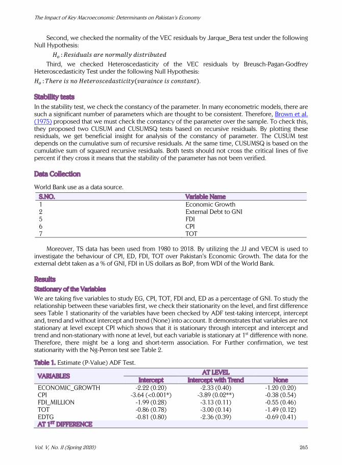
We are taking five variables to study EG, CPI, TOT, FDI and, ED as a percentage of GNI. To study the relationship between these variables first, we check their stationarity on the level, and first difference sees Table 1 stationarity of the variables have been checked by ADF test-taking intercept, intercept and, trend and without intercept and trend (None) into account. It demonstrates that variables are not stationary at level except CPI which shows that it is stationary through intercept and intercept and trend and non-stationary with none at level, but each variable is stationary at 1st difference with none. Therefore, there might be a long and short-term association. For Further confirmation, we test stationarity with the Ng-Perron test see Table 2.

Table 1. Estimate (P-Value) ADF Test.

VARIABLES AT LEVEL

Intercept Intercept with Trend None ECONOMIC_GROWTH -2.22 (0.20) -2.33 (0.40) -1.20 (0.20) CPI -3.64 (<0.001*) -3.89 (0.02**) -0.38 (0.54) FDI_MILLION -1.99 (0.28) -3.13 (0.11) -0.55 (0.46) TOT -0.86 (0.78) -3.00 (0.14) -1.49 (0.12) EDTG -0.81 (0.80) -2.36 (0.39) -0.69 (0.41) AT 1ST DIFFERENCE



* Significance at 1%, **Significance at 5%

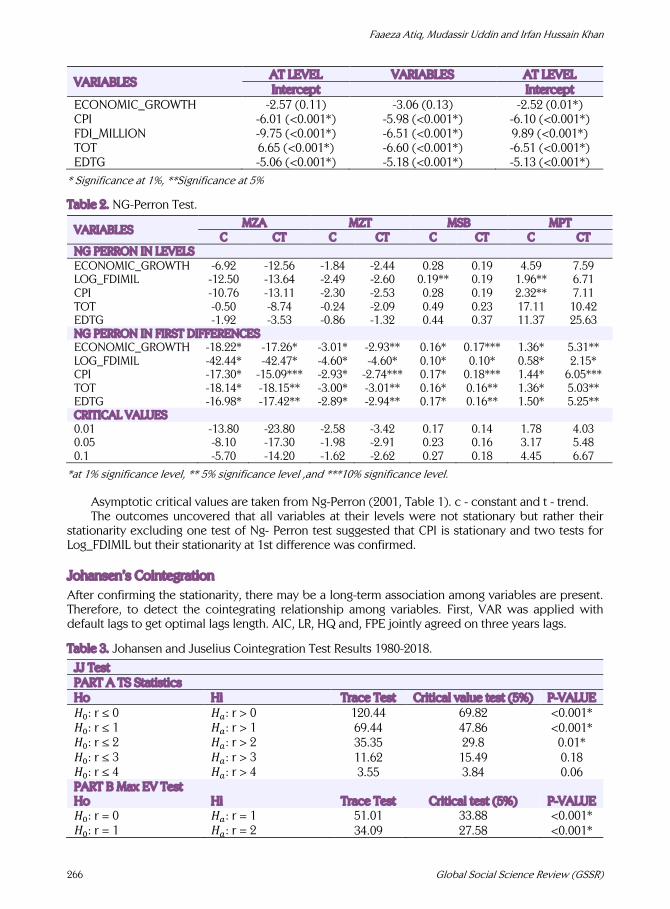
Table 2. NG-Perron Test.

VARIABLES MZA MZT MSB MPT

C CT C CT C CT C CT NG PERRON IN LEVELS ECONOMIC_GROWTH -6.92 -12.56 -1.84 -2.44 0.28 0.19 4.59 7.59 LOG_FDIMIL -12.50 -13.64 -2.49 -2.60 0.19** 0.19 1.96** 6.71 CPI -10.76 -13.11 -2.30 -2.53 0.28 0.19 2.32** 7.11 TOT -0.50 -8.74 -0.24 -2.09 0.49 0.23 17.11 10.42 EDTG -1.92 -3.53 -0.86 -1.32 0.44 0.37 11.37 25.63 NG PERRON IN FIRST DIFFERENCES ECONOMIC_GROWTH -18.22* -17.26* -3.01* -2.93** 0.16* 0.17*** 1.36* 5.31** LOG_FDIMIL -42.44* -42.47* -4.60* -4.60* 0.10* 0.10* 0.58* 2.15* CPI -17.30* -15.09*** -2.93* -2.74*** 0.17* 0.18*** 1.44* 6.05*** TOT -18.14* -18.15** -3.00* -3.01** 0.16* 0.16** 1.36* 5.03** EDTG -16.98* -17.42** -2.89* -2.94** 0.17* 0.16** 1.50* 5.25** CRITICAL VALUES 0.01 -13.80 -23.80 -2.58 -3.42 0.17 0.14 1.78 4.03 0.05 -8.10 -17.30 -1.98 -2.91 0.23 0.16 3.17 5.48 0.1 -5.70 -14.20 -1.62 -2.62 0.27 0.18 4.45 6.67

*at 1% significance level, ** 5% significance level ,and ***10% significance level.

Asymptotic critical values are taken from Ng-Perron (2001, Table 1). c - constant and t - trend. The outcomes uncovered that all variables at their levels were not stationary but rather their

stationarity excluding one test of Ng- Perron test suggested that CPI is stationary and two tests for Log_FDIMIL but their stationarity at 1st difference was confirmed. Johansen’s Cointegration After confirming the stationarity, there may be a long-term association among variables are present. Therefore, to detect the cointegrating relationship among variables. First, VAR was applied with default lags to get optimal lags length. AIC, LR, HQ and, FPE jointly agreed on three years lags.

Table 3. Johansen and Juselius Cointegration Test Results 1980-2018.

JJ Test PART A TS Statistics Ho Hi Trace Test Critical value test (5%) P-VALUE 𝐻8: r ≤ 0 𝐻": r > 0 120.44 69.82 <0.001* 𝐻8: r ≤ 1 𝐻": r > 1 69.44 47.86 <0.001* 𝐻8: r ≤ 2 𝐻": r > 2 35.35 29.8 0.01* 𝐻8: r ≤ 3 𝐻": r > 3 11.62 15.49 0.18 𝐻8: r ≤ 4 𝐻": r > 4 3.55 3.84 0.06 PART B Max EV Test Ho Hi Trace Test Critical test (5%) P-VALUE 𝐻8: r = 0 𝐻": r = 1 51.01 33.88 <0.001* 𝐻8: r = 1 𝐻": r = 2 34.09 27.58 <0.001*

VARIABLES AT LEVEL VARIABLES AT LEVEL Intercept Intercept

ECONOMIC_GROWTH -2.57 (0.11) -3.06 (0.13) -2.52 (0.01*) CPI -6.01 (<0.001*) -5.98 (<0.001*) -6.10 (<0.001*) FDI_MILLION -9.75 (<0.001*) -6.51 (<0.001*) 9.89 (<0.001*) TOT 6.65 (<0.001*) -6.60 (<0.001*) -6.51 (<0.001*) EDTG -5.06 (<0.001*) -5.18 (<0.001*) -5.13 (<0.001*)



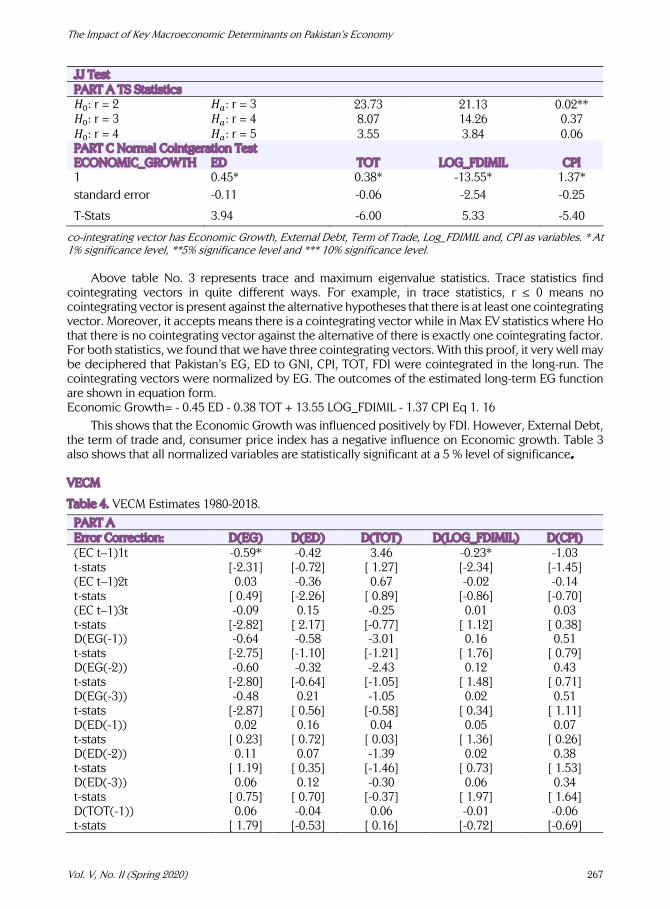
JJ Test PART A TS Statistics 𝐻8: r = 2 𝐻": r = 3 23.73 21.13 0.02** 𝐻8: r = 3 𝐻": r = 4 8.07 14.26 0.37 𝐻8: r = 4 𝐻": r = 5 3.55 3.84 0.06 PART C Normal Cointgeration Test ECONOMIC_GROWTH ED TOT LOG_FDIMIL CPI 1 0.45* 0.38* -13.55* 1.37* standard error -0.11 -0.06 -2.54 -0.25

T-Stats 3.94 -6.00 5.33 -5.40

co-integrating vector has Economic Growth, External Debt, Term of Trade, Log_FDIMIL and, CPI as variables. * At 1% significance level, **5% significance level and *** 10% significance level.

Above table No. 3 represents trace and maximum eigenvalue statistics. Trace statistics find cointegrating vectors in quite different ways. For example, in trace statistics, r ≤ 0 means no cointegrating vector is present against the alternative hypotheses that there is at least one cointegrating vector. Moreover, it accepts means there is a cointegrating vector while in Max EV statistics where Ho that there is no cointegrating vector against the alternative of there is exactly one cointegrating factor. For both statistics, we found that we have three cointegrating vectors. With this proof, it very well may be deciphered that Pakistan’s EG, ED to GNI, CPI, TOT, FDI were cointegrated in the long-run. The cointegrating vectors were normalized by EG. The outcomes of the estimated long-term EG function are shown in equation form. Economic Growth= - 0.45 ED - 0.38 TOT + 13.55 LOG_FDIMIL - 1.37 CPI Eq 1. 16

This shows that the Economic Growth was influenced positively by FDI. However, External Debt, the term of trade and, consumer price index has a negative influence on Economic growth. Table 3 also shows that all normalized variables are statistically significant at a 5 % level of significance. VECM

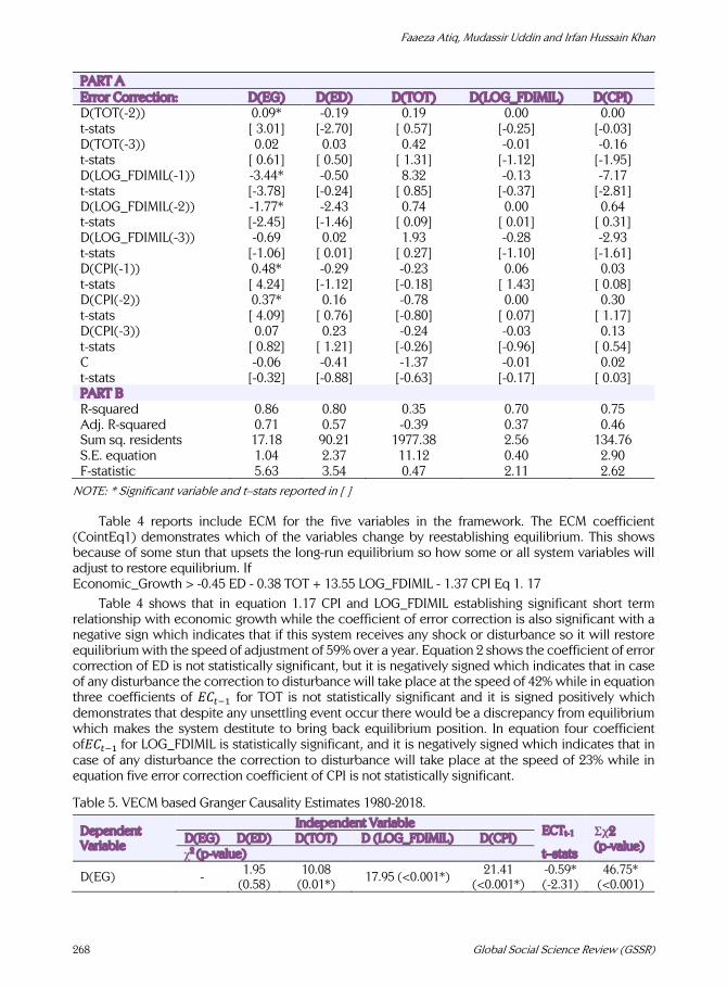
Table 4. VECM Estimates 1980-2018.

PART A Error Correction: D(EG) D(ED) D(TOT) D(LOG_FDIMIL) D(CPI) (EC t–1)1t -0.59* -0.42 3.46 -0.23* -1.03 t-stats [-2.31] [-0.72] [ 1.27] [-2.34] [-1.45] (EC t–1)2t 0.03 -0.36 0.67 -0.02 -0.14 t-stats [ 0.49] [-2.26] [ 0.89] [-0.86] [-0.70] (EC t–1)3t -0.09 0.15 -0.25 0.01 0.03 t-stats [-2.82] [ 2.17] [-0.77] [ 1.12] [ 0.38] D(EG(-1)) -0.64 -0.58 -3.01 0.16 0.51 t-stats [-2.75] [-1.10] [-1.21] [ 1.76] [ 0.79] D(EG(-2)) -0.60 -0.32 -2.43 0.12 0.43 t-stats [-2.80] [-0.64] [-1.05] [ 1.48] [ 0.71] D(EG(-3)) -0.48 0.21 -1.05 0.02 0.51 t-stats [-2.87] [ 0.56] [-0.58] [ 0.34] [ 1.11] D(ED(-1)) 0.02 0.16 0.04 0.05 0.07 t-stats [ 0.23] [ 0.72] [ 0.03] [ 1.36] [ 0.26] D(ED(-2)) 0.11 0.07 -1.39 0.02 0.38 t-stats [ 1.19] [ 0.35] [-1.46] [ 0.73] [ 1.53] D(ED(-3)) 0.06 0.12 -0.30 0.06 0.34 t-stats [ 0.75] [ 0.70] [-0.37] [ 1.97] [ 1.64] D(TOT(-1)) 0.06 -0.04 0.06 -0.01 -0.06 t-stats [ 1.79] [-0.53] [ 0.16] [-0.72] [-0.69]



PART A Error Correction: D(EG) D(ED) D(TOT) D(LOG_FDIMIL) D(CPI) D(TOT(-2)) 0.09* -0.19 0.19 0.00 0.00 t-stats [ 3.01] [-2.70] [ 0.57] [-0.25] [-0.03] D(TOT(-3)) 0.02 0.03 0.42 -0.01 -0.16 t-stats [ 0.61] [ 0.50] [ 1.31] [-1.12] [-1.95] D(LOG_FDIMIL(-1)) -3.44* -0.50 8.32 -0.13 -7.17 t-stats [-3.78] [-0.24] [ 0.85] [-0.37] [-2.81] D(LOG_FDIMIL(-2)) -1.77* -2.43 0.74 0.00 0.64 t-stats [-2.45] [-1.46] [ 0.09] [ 0.01] [ 0.31] D(LOG_FDIMIL(-3)) -0.69 0.02 1.93 -0.28 -2.93 t-stats [-1.06] [ 0.01] [ 0.27] [-1.10] [-1.61] D(CPI(-1)) 0.48* -0.29 -0.23 0.06 0.03 t-stats [ 4.24] [-1.12] [-0.18] [ 1.43] [ 0.08] D(CPI(-2)) 0.37* 0.16 -0.78 0.00 0.30 t-stats [ 4.09] [ 0.76] [-0.80] [ 0.07] [ 1.17] D(CPI(-3)) 0.07 0.23 -0.24 -0.03 0.13 t-stats [ 0.82] [ 1.21] [-0.26] [-0.96] [ 0.54] C -0.06 -0.41 -1.37 -0.01 0.02 t-stats [-0.32] [-0.88] [-0.63] [-0.17] [ 0.03] PART B R-squared 0.86 0.80 0.35 0.70 0.75 Adj. R-squared 0.71 0.57 -0.39 0.37 0.46 Sum sq. residents 17.18 90.21 1977.38 2.56 134.76 S.E. equation 1.04 2.37 11.12 0.40 2.90 F-statistic 5.63 3.54 0.47 2.11 2.62

NOTE: * Significant variable and t–stats reported in [ ]

Table 4 reports include ECM for the five variables in the framework. The ECM coefficient (CointEq1) demonstrates which of the variables change by reestablishing equilibrium. This shows because of some stun that upsets the long-run equilibrium so how some or all system variables will adjust to restore equilibrium. If Economic_Growth > -0.45 ED - 0.38 TOT + 13.55 LOG_FDIMIL - 1.37 CPI Eq 1. 17

Table 4 shows that in equation 1.17 CPI and LOG_FDIMIL establishing significant short term relationship with economic growth while the coefficient of error correction is also significant with a negative sign which indicates that if this system receives any shock or disturbance so it will restore equilibrium with the speed of adjustment of 59% over a year. Equation 2 shows the coefficient of error correction of ED is not statistically significant, but it is negatively signed which indicates that in case of any disturbance the correction to disturbance will take place at the speed of 42% while in equation three coefficients of 𝐸𝐶#$% for TOT is not statistically significant and it is signed positively which demonstrates that despite any unsettling event occur there would be a discrepancy from equilibrium which makes the system destitute to bring back equilibrium position. In equation four coefficient of𝐸𝐶#$%for LOG_FDIMIL is statistically significant, and it is negatively signed which indicates that in case of any disturbance the correction to disturbance will take place at the speed of 23% while in equation five error correction coefficient of CPI is not statistically significant.

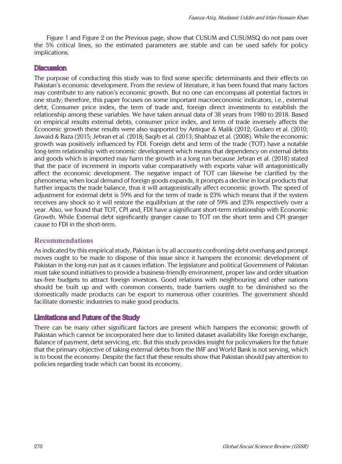
Table 5. VECM based Granger Causality Estimates 1980-2018.

Dependent Variable

Independent Variable ECTt-1 Σχ2

(p-value) D(EG) D(ED) D(TOT) D (LOG_FDIMIL) D(CPI) ꭓ2 (p-value) t–stats

D(EG) - 1.95 (0.58)

10.08 (0.01*)

17.95 (<0.001*) 21.41 (<0.001*)

-0.59* (-2.31)

46.75* (<0.001)



Dependent Variable

Independent Variable ECTt-1 Σχ2

(p-value) D(EG) D(ED) D(TOT) D (LOG_FDIMIL) D(CPI) ꭓ2 (p-value) t–stats

D(ED) 3.45 (0.32)

- 11.37 (<0.001*)

2.42 (0.49)

6.45 (0.09)

-0.42 (-0.72)

27.87* (<0.001)

D(TOT) 1.63 (0.65)

2.19 (0.53)

- 1.00 (0.80)

0.95 (0.81)

3.45 (1.27)

7.52 (0.82)

D(LOG_FDIMIL) 4.31

(0.22) 7.09

(0.07) 1.76

(0.62) - 4.51

(0.21) -0.23* (-2.34)

15.66 (0.20)

D(CPI) 1.33

(0.72) 4.70

(0.19) 5.18

(0.15) 11.52

(<0.001*) - -1.03

(-1.45) 21.60* (0.04)

NOTE: * Significance at 1%, ** at 5% and *** at 10% level.

As we see our variables are cointegrated so there should be a causal relationship existed. Long term Causal relationship checked by Lagged error correction term with t-values in parenthesis see Table 5 reports p-values of chi-square for individual short-term causality while p-value tells the significance of overall short-term causality. The outcomes demonstrated that lagged residual term of D(EG) is statistically significant that shown a stable long-term association among explained and explanatory variables. We can entail that due to the significant long-term relationship; variables may not deviate too much and concurrence can be adept. Whereas statics value for the lagged term was affirmed that t-statistics & significant Σχ2 means that short-run causality, as well as, we see significant individual causality too, i.e. D(LOG_FDIMIL) granger cause to D(EG) and D(CPI) also granger Cause to D(EG) and D(TOT) granger cause to D(EG). In the case of D(ED) as a dependent variable, there is no significant long-run causality, but Σχ2 were statistically significant therefore we can conclude D(TOT) granger cause to D(ED) on the short-run whereas for D(TOT) and D(LOG_FDIMIL) as dependent variable no channels of short-run causalities were found, but D(LOG_FDIMIL) has significant long-run causality. D(CPI) as dependent Variable has significant short-run causality Diagnostic Tests Table 6. Diagnostic Tests.

Test Statistics Prob. Results LM-stat 0.10 There is no serial correlation in Residuals Jarque-Bera 0.37 Residuals are normally distributed Chi-square 0.55 There is no heteroscedasticity

Table 6 shows diagnostic tests for residuals. Our results show these residuals are free from serial

correlation and have homoscedasticity (same variance) as well as they normally distributed, which validates that the fitted model can give us useful insights. Stability Tests

Figure 1 Figure 2



Figure 1 and Figure 2 on the Previous page, show that CUSUM and CUSUMSQ do not pass over the 5% critical lines, so the estimated parameters are stable and can be used safely for policy implications. Discussion The purpose of conducting this study was to find some specific determinants and their effects on Pakistan’s economic development. From the review of literature, it has been found that many factors may contribute to any nation’s economic growth. But no one can encompass all potential factors in one study; therefore, this paper focuses on some important macroeconomic indicators, i.e., external debt, Consumer price index, the term of trade and, foreign direct investments to establish the relationship among these variables. We have taken annual data of 38 years from 1980 to 2018. Based on empirical results external debts, consumer price index, and term of trade inversely affects the Economic growth these results were also supported by Antique & Malik (2012; Gudaro et al. (2010; Jawaid & Raza (2015; Jebran et al. (2018; Saqib et al. (2013; Shahbaz et al. (2008). While the economic growth was positively influenced by FDI. Foreign debt and term of the trade (TOT) have a notable long-term relationship with economic development which means that dependency on external debts and goods which is imported may harm the growth in a long run because Jebran et al. (2018) stated that the pace of increment in imports value comparatively with exports value will antagonistically affect the economic development. The negative impact of TOT can likewise be clarified by the phenomena; when local demand of foreign goods expands, it prompts a decline in local products that further impacts the trade balance, thus it will antagonistically affect economic growth. The speed of adjustment for external debt is 59% and for the term of trade is 23% which means that if the system receives any shock so it will restore the equilibrium at the rate of 59% and 23% respectively over a year. Also, we found that TOT, CPI and, FDI have a significant short-term relationship with Economic Growth. While External debt significantly granger cause to TOT on the short term and CPI granger cause to FDI in the short-term. Recommendations As indicated by this empirical study, Pakistan is by all accounts confronting debt overhang and prompt moves ought to be made to dispose of this issue since it hampers the economic development of Pakistan in the long-run just as it causes inflation. The legislature and political Government of Pakistan must take sound initiatives to provide a business-friendly environment, proper law and order situation tax-free budgets to attract foreign investors. Good relations with neighbouring and other nations should be built up and with common consents, trade barriers ought to be diminished so the domestically made products can be export to numerous other countries. The government should facilitate domestic industries to make good products. Limitations and Future of the Study

There can be many other significant factors are present which hampers the economic growth of Pakistan which cannot be incorporated here due to limited dataset availability like foreign exchange, Balance of payment, debt servicing, etc. But this study provides insight for policymakers for the future that the primary objective of taking external debts from the IMF and World Bank is not serving, which is to boost the economy. Despite the fact that these results show that Pakistan should pay attention to policies regarding trade which can boost its economy.



References Abbas, Q., S. Akbar, A. S. Nasir and H. A. Ullah (2011). "Impact of foreign direct investment on the

gross domestic product (A case of SAARC countries)." Global Journal of Management and Business Research 11(8).

Abdalla, M. and H. H. Abdelbaki (2014). "Determinants of economic growth in GCC economies." Asian Journal of Research in Business Economics and Management 4(11): 46-62.

Agrawal, G. (2015). "Foreign direct investment and economic growth in BRICS economies: A panel data analysis." Journal of Economics, Business and Management 3(4): 421-424.

Agrawal, G. and M. A. Khan (2011). "Impact of FDI on GDP: A comparative study of China and India." International Journal of Business and Management 6(10): 71.

Akram, N. (2017). "Role of public debt in the economic growth of Sri Lanka: An ARDL Approach." Pakistan Journal of Applied Economics 27(2): 189-212.

Arshad, Z., S. Aslam, M. Fatima and A. Muzaffar (2015). "Debt Accumulation and Economic Growth: Empirical Evidence from Pakistan Economy." International Journal of Economics and Empirical Research (IJEER) 3(8): 405-410.

Asghar, N., S. Nasreen and H. Rehman (2011). "Relationship between FDI and economic growth in selected Asian countries: A panel data analysis." Review of Economics & Finance 2: 84-96.

Atique, R. and K. Malik (2012). "Impact of domestic and external debt on the economic growth of Pakistan." World Applied Sciences Journal 20(1): 120-129.

Brooks, C. (2008). "Univariatetime series modelling and forecasting." Introductory Econometrics for Finance. 2nd Ed. Cambridge University Press. Cambridge, Massachusetts.

Brown, R. L., J. Durbin and J. M. Evans (1975). "Techniques for testing the constancy of regression relationships over time." Journal of the Royal Statistical Society: Series B (Methodological) 37(2): 149-163.

Chaudhry, I. S., S. Iffat and F. Farooq (2017). "Foreign Direct Investment, External Debt and Economic Growth: Evidence from some Selected Developing Countries." Review of Economics and Development Studies 3(2): 111-124.

DeJong, D. N., J. C. Nankervis, N. E. Savin and C. H. Whiteman (1992). "Integration versus trend stationary in time series." Econometrica: Journal of the Econometric Society: 423-433.

Eichengreen, B. and R. Portes (1986). "Debt and Default in the 1930s: Causes and Consequences." European Economic Review 30(3): 599-640.

Engle, R. F. and C. W. Granger (1987). "Co-integration and error correction: representation, estimation, and testing." Econometrica: journal of the Econometric Society: 251-276.

Ferraro, V. and M. Rosser (1994). "Global debt and third world development." Granger, C. W. (1988). "Some recent development in a concept of causality." Journal of econometrics

39(1-2): 199-211. Granger, C. W., P. Newbold and J. Econom (1974). "Spurious regressions in econometrics." Baltagi,

Badi H. A Companion of Theoretical Econometrics: 557-561. Griffin, K. B. and J. L. Enos (1970). "Foreign assistance: objectives and consequences." Economic

development and cultural change 18(3): 313-327. Gudaro, A. M., I. U. Chhapra and S. A. Shaikh (2010). "Impact of foreign direct investment on economic

growth: A case study of Pakistan." IBT JOURNAL OF BUSINESS STUDIES (JBS) 6(2). Gul, S., I. Mohammad and A. Amin (2015). "Need and Economic Impact Specific Empirical

Assessment of Foreign Capital Inflows to Less Developed Countries (A Case Of Pakistan: 1981-2012)." FWU Journal of Social Sciences 9(1): 141.

Harris, R. and R. Sollis (2003). Applied time series modelling and forecasting, Wiley. Havi, E. D. K., P. Enu, F. Osei-Gyimah, P. Attah-Obeng and C. Opoku (2013). "Macroeconomic

determinants of economic growth in Ghana: Cointegration approach." European Scientific Journal 9(19).

Iqbal, Z. and G. M. Zahid (1998). "Macroeconomic determinants of economic growth in Pakistan." The Pakistan Development Review: 125-148.



Jawaid, S. T. and S. A. Raza (2015). "Do terms of trade and its volatility matter? Evidence from economic escalation of China." Journal of Transnational Management 20(1): 3-30.

Jebran, K., A. Iqbal, Z. U. R. Rao and A. Ali (2018). "Effects of terms of trade on economic growth of Pakistan." Foreign Trade Review 53(1): 1-11.

Johansen, S. (1995). Likelihood-based inference in cointegrated vector autoregressive models, Oxford University Press on Demand.

Johansen, S. and K. Juselius (1990). "Maximum likelihood estimation and inference on cointegration—with applications to the demand for money." Oxford Bulletin of Economics and statistics 52(2): 169-210.

Kalumbu, S. A. and J. P. S. Sheefeni (2014). "Terms of trade and economic growth in Namibia." International Review of Research in Emerging Markets and the Global Economy 1(3): 90-101.

Khachoo, A. Q. and M. I. Khan (2012). "Determinants of FDI inflows to developing countries: a panel data analysis."

Mehmood, K. A. and S. Hassan (2015). "A study on mapping out alliance between economic growth and foreign direct investment in Pakistan." Asian Social Science 11(15): 113.

Ng, S. and P. Perron (2001). "A note on the selection of time series models." Working Papers in Economics: 116.

Pradhan, R. P. (2009). "The FDI-led-growth hypothesis in ASEAN-5 countries: Evidence from cointegrated panel analysis." International Journal of Business and Management 4(12): 153-164.

Saqib, D., M. Masnoon and N. Rafique (2013). "Impact of foreign direct investment on economic growth of Pakistan."

Sattar, A. (2015). "The Impact Foreign Direct Investment on Economic Growth in Pakistan Since 1980." Journal of Economics and Sustainable Development 6(7): 132-141.

Shahbaz, M., K. Ahmad and A. Chaudhary (2008). "Economic growth and its determinants in Pakistan." The Pakistan Development Review: 471-486.

Siddique, A., E. Selvanathan and S. Selvanathan (2015). The impact of external debt on economic growth: Empirical evidence from highly indebted poor countries, University of Western Australia, Economics.

Sulaiman, L. and B. Azeez (2012). "Effect of external debt on economic growth of Nigeria." Journal of Economics and sustainable development 3(8): 71-79.

Tiruneh, M. W. (2004). "An empirical investigation into the determinants of external indebtedness." Prague economic papers 3(2004): 261-277.

Tsay, R. S. (2005). Analysis of financial time series, John wiley & sons. Wong, H. T. (2010). "Terms of trade and economic growth in Japan and Korea: an empirical analysis."

Empirical Economics 38(1): 139-158. Zafar, S. and M. S. Butt (2008). "Impact of trade liberalization on external debt burden: econometric

evidence from Pakistan." Zakari, Y. and H. Mohammed (2012). "Does FDI cause economic growth? Evidence from selected

countries in Africa and Asia." Zeb, N., F. Qiang and S. Rauf (2013). "Role of foreign direct investment in economic growth of

Pakistan." International Journal of Economics and Finance 6(1): 32.

25 the impact of some macroeconomic determinants - faaeza atiq

Documents