24/05/2007 maria adler university of kaiserslautern department of mathematics 1 hyperbolic processes...
Post on 20-Dec-2015
212 views
TRANSCRIPT

24/05/2007
Maria AdlerUniversity of KaiserslauternDepartment of Mathematics 1
Hyperbolic Processes in Finance
Alternative Models for Asset Prices

224/05/2007
Hyperbolic Processes in Finance
Outline
The Black-Scholes Model Fit of the BS Model to Empirical Data Hyperbolic Distribution Hyperbolic Lévy Motion Hyperbolic Model of the Financial Market Equivalent Martingale Measure Option Pricing in the Hyperbolic Model Fit of the Hyperbolic Model to Empirical Data Conclusion

324/05/2007
Hyperbolic Processes in Finance
The Black-Scholes Model
0ttP price process of a security described by the SDE
tt
ttt
WtPP
dWPdtPdP
2exp
2
0 :
:
:0
0
ttW
volatility
drift
Brownian motion
rtBB
dtBrdB
B
t
ttt
tt
exp0
0
:0ttr interest rate
price process of a risk-free bond

424/05/2007
Hyperbolic Processes in Finance
Brownian motion has continuous paths stationary and independent increments market in this model is complete
allows duplication of the cash flow of
derivative securities and pricing by
arbitrage principle
The Black-Scholes Model
524/05/2007
Hyperbolic Processes in Finance
statistical analysis of daily stock-price data from 10 of the DAX30 companies
time period: 2 Oct 1989 – 30 Sep 1992 (3 years)
745 data points each for the returns
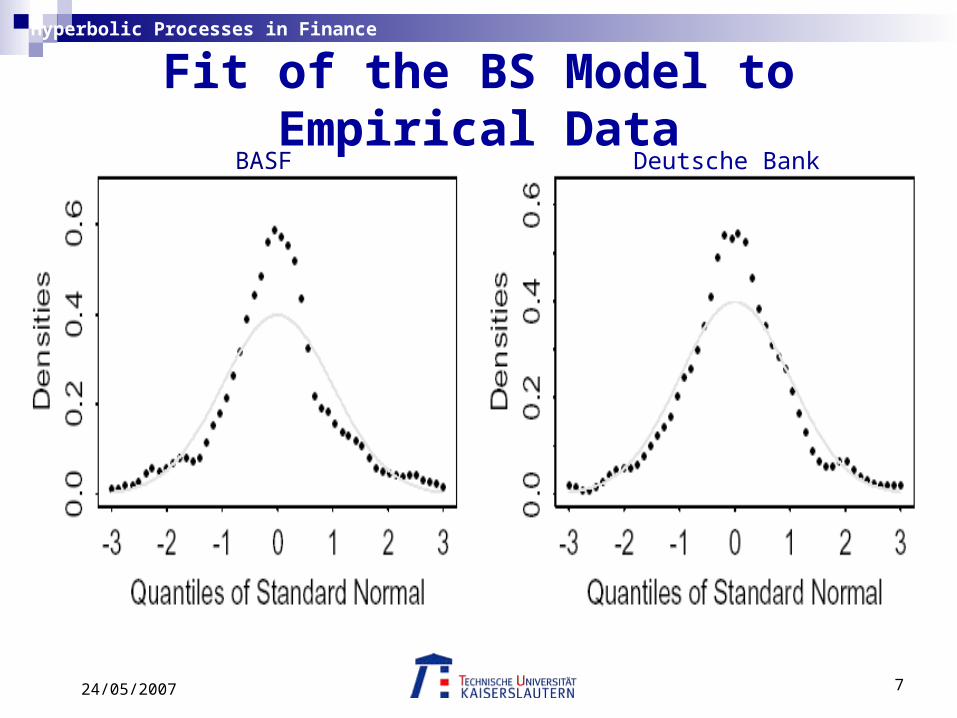
Result: assumption of Normal distribution underlying the
Black- Scholes model does not provide a good fit to
the market data
Fit of the BS Model to Empirical Data

624/05/2007
Hyperbolic Processes in Finance
Fit of the BS Model to Empirical Data
Quantile-Quantile plots & density-plots for the returns of BASF and Deutsche Bank to test goodness of fit:Fig. 4, E./K., p.7
724/05/2007
Hyperbolic Processes in Finance
Fit of the BS Model to Empirical Data
BASF Deutsche Bank

824/05/2007
Hyperbolic Processes in Finance
Brownian motion represents the net random effect of the various factors of influence in the economic environment
(shocks; price-sensitive information)
actually, one would expect this effect to be discontinuous, as the individual shocks arrive
indeed, price processes are discontinuous looked at closely enough (discrete ´shocks´)
Fit of the BS Model to Empirical Data

924/05/2007
Hyperbolic Processes in Finance
Fit of the BS Model to Empirical Data
Fig. 1, E./K., p.4
typical path of a Brownian motion continuousthe qualitative picture does not change if we change the time-scale,
due to self-similarity property
08.0,5.0,1000 P
0,2 ctcWtcW
1024/05/2007
Hyperbolic Processes in Finance
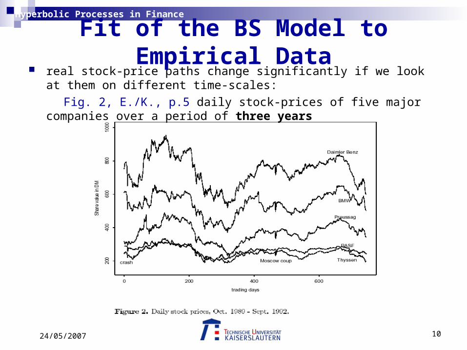
real stock-price paths change significantly if we look at them on different time-scales:
Fig. 2, E./K., p.5 daily stock-prices of five major companies over a period of three years
Fit of the BS Model to Empirical Data

1124/05/2007
Hyperbolic Processes in Finance
Fig. 3, E./K., p.6 path, showing price changes of the Siemens stock during a single day
Fit of the BS Model to Empirical Data
1224/05/2007
Hyperbolic Processes in Finance
Aim: to model financial data more precisely than with the BS model
find a more flexible distribution than the normal distr.
find a process with stationary and independent increments (similar
to the Brownian motion), but with a more general distr.
this leads to models based on Lévy processes
in particular: Hyperbolic processes
B./K. and E./K. showed that the Hyperbolic model is a more realistic market model than the Black-Scholes model, providing a better fit to stock prices than the normal distribution, especially when looking at time periods of a single day
Fit of the BS Model to Empirical Data

1324/05/2007
Hyperbolic Processes in Finance
Hyperbolic Distribution
introduced by Barndorff-Nielsen in 1977
used in various scientific fields: - modeling the distribution of the grain size of sand - modeling of turbulence - use in statistical physics
Eberlein and Keller introduced hyperbolic distribution functions into finance

1424/05/2007
Hyperbolic Processes in Finance
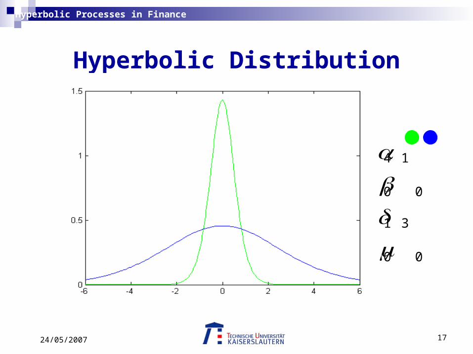
Density of the Hyperbolic distribution:
Hyperbolic Distribution
xxK
xhyp 22
221
22
,,, exp2
:1K modified Bessel function with index 1
characterized by four parameters:
:0 tail decay; behavior of density for x:0 skewness / asymmetry
shape
:R location
:0 scale

1524/05/2007
Hyperbolic Processes in Finance
Hyperbolic DistributionDensity-plots for different parameters:
1 9 0
0 0 0
1 1 1
0 0 0

1624/05/2007
Hyperbolic Processes in Finance
Hyperbolic Distribution
4 4
5 0
6 1
3 2
1724/05/2007
Hyperbolic Processes in Finance
Hyperbolic Distribution
4 1
0 0
1 3
0 0

1824/05/2007
Hyperbolic Processes in Finance
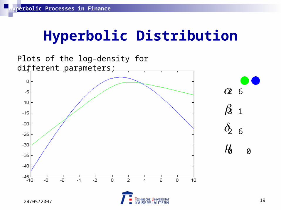
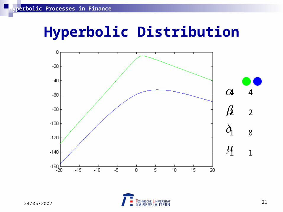
the log-density is a hyperbola ( reason for the name)
this leads to thicker tails than for the normal distribution, where the log-density is a parabola
Hyperbolic Distribution
xx 22 0
:, slopes of the asymptotics
: location
: curvature near the mode
1924/05/2007
Hyperbolic Processes in Finance
Hyperbolic Distribution
Plots of the log-density for different parameters:
2 6
3 1
2 6
0 0

2024/05/2007
Hyperbolic Processes in Finance
Hyperbolic Distribution
2 2
3 1
2 10
0 0
2124/05/2007
Hyperbolic Processes in Finance
Hyperbolic Distribution
4 4
2 2
1 8
1 1
2224/05/2007
Hyperbolic Processes in Finance
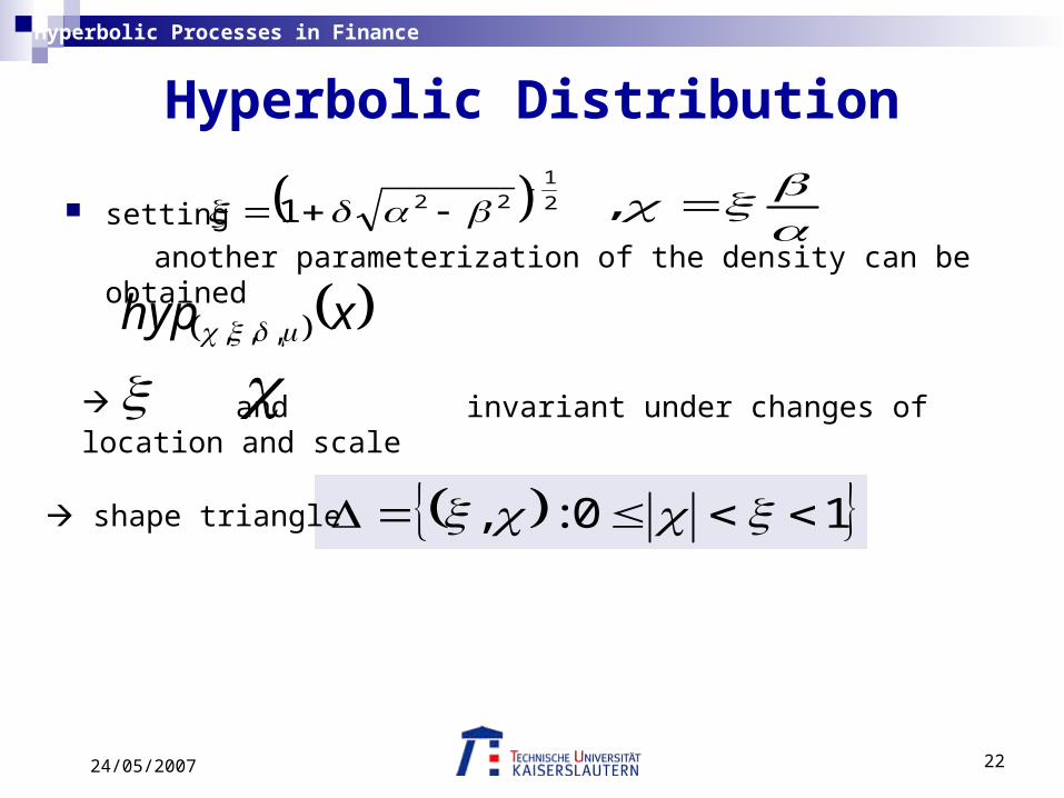
setting
another parameterization of the density can be obtained
Hyperbolic Distribution
2
1221
,
xhyp ,,,
and invariant under changes of location and scale
10:, shape triangle

2324/05/2007
Hyperbolic Processes in Finance
Hyperbolic Distribution
Fig. 6, E./K., p.13
generalized inverse Gaussian
generalized inverse Gaussian
2424/05/2007
Hyperbolic Processes in Finance
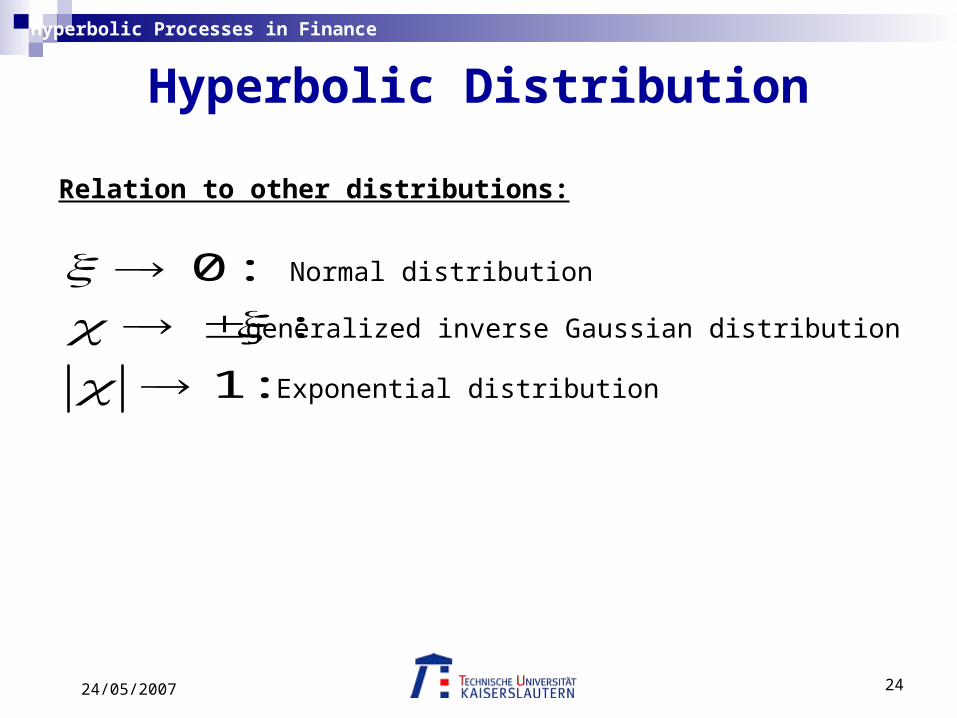
Relation to other distributions:
Hyperbolic Distribution
:1
:
:0
Normal distribution
generalized inverse Gaussian distribution
Exponential distribution

2524/05/2007
Hyperbolic Processes in Finance
Representation as a mean-variance mixture of normals:Barndorff-Nielsen and Halgreen (1977)
the mixing distribution is the generalized inverse Gaussian with density
Hyperbolic Distribution
xx
Kxd IG
1
1 2
1exp
2
• consider a normal distribution with mean and variance :2 2
22 , N
• such that is a random variable with distribution 2 xd IG
• the resulting mixture is a hyperbolic distribution xhyp ,,,
2624/05/2007
Hyperbolic Processes in Finance
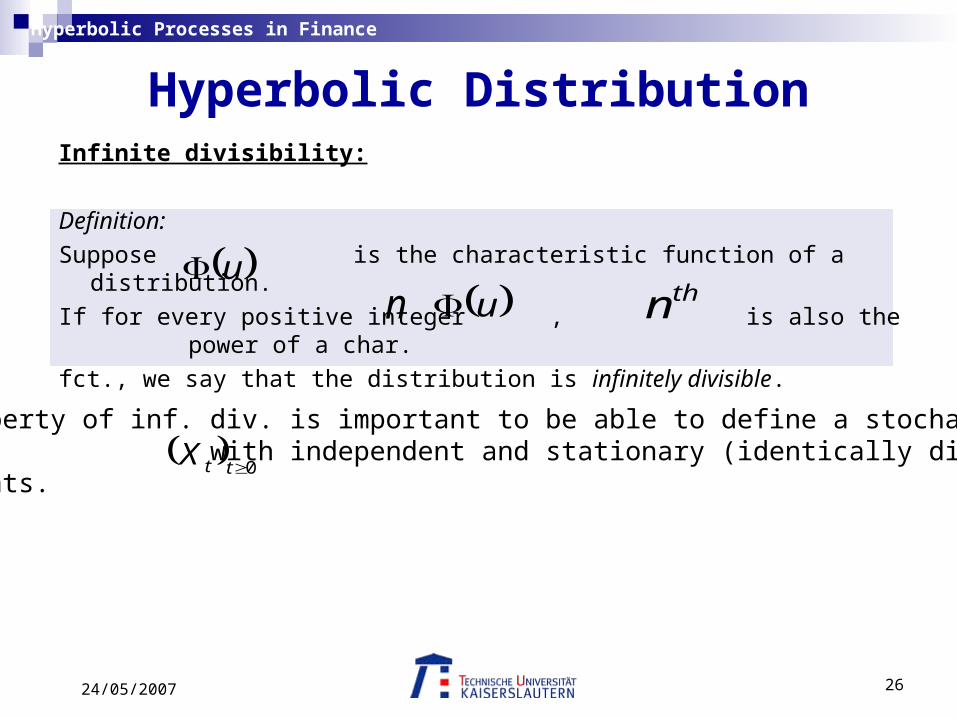
Infinite divisibility:
Definition:
Suppose is the characteristic function of a distribution.
If for every positive integer , is also the power of a char.
fct., we say that the distribution is infinitely divisible.
Hyperbolic Distribution
u u thnn
The property of inf. div. is important to be able to define a stochasticprocess with independent and stationary (identically distr.)increments.
0ttX
2724/05/2007
Hyperbolic Processes in Finance
Barndorff-Nielsen and Halgreen showed that the generalized inverse Gaussian distribution is infinitely divisible.
Since we obtain the hyperbolic distribution as a mean-variance mixture from the gen. inv. Gaussian distr. as a mixing distribution, this transfers infinite divisibility to the hyperbolic distribution.
The hyperbolic distribution is infinitely divisible and we can define the hyperbolic Lévy process with the required properties.
Hyperbolic Distribution

2824/05/2007
Hyperbolic Processes in Finance
To fit empirical data it suffices to concentrate on the centered
symmetric case.
Hence, consider the hyperbolic density
Hyperbolic Distribution 0
0/0
1
1
0,
,1exp2
1
2
2
122
2
1,
x
Kxhyp

2924/05/2007
Hyperbolic Processes in Finance
Characteristic function:
The corresponding char. fct. to is given by
Hyperbolic Distribution
xhyp ,
222
2221
1
,;u
uK
Kuu
• All moments of the hyperbolic distribution exist.
3024/05/2007
Hyperbolic Processes in Finance
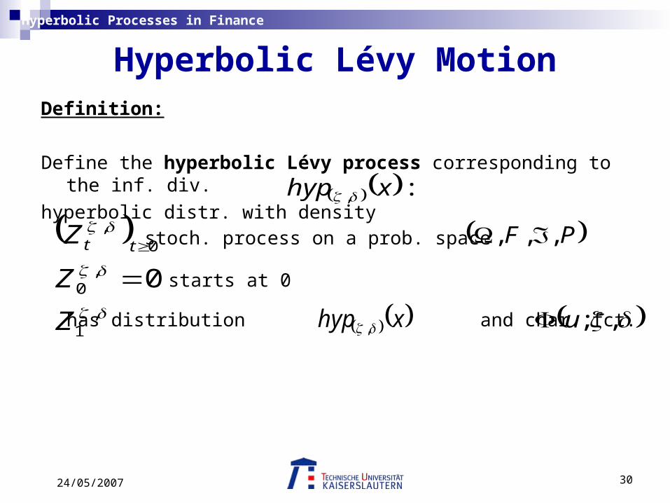
Hyperbolic Lévy MotionDefinition:
Define the hyperbolic Lévy process corresponding to the inf. div.
hyperbolic distr. with density :, xhyp
,1
,0
0,
0
Z
Z
Z tt
stoch. process on a prob. space
starts at 0
has distribution and char. fct.
PF ,,,
xhyp , ,;u

3124/05/2007
Hyperbolic Processes in Finance
Hyperbolic Lévy Motion
For the char. fct. of we get
,tZ
,tZ
ttiuZ uueE t
,;,;,
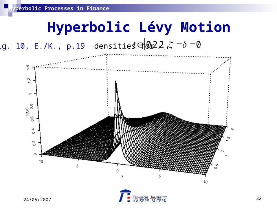
The density of is given by the Fourier Inversion formula:
duuuxxf tt
,;cos1
0
,
only has hyperbolic distribution ,1Z
0t
3224/05/2007
Hyperbolic Processes in Finance
Fig. 10, E./K., p.19 densities for 0,2,2.0 t
Hyperbolic Lévy Motion
3324/05/2007
Hyperbolic Processes in Finance
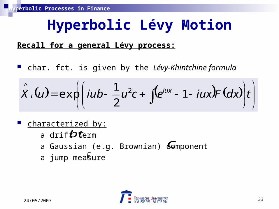
Recall for a general Lévy process:
char. fct. is given by the Lévy-Khintchine formula
characterized by:
a drift term
a Gaussian (e.g. Brownian) component
a jump measure
Hyperbolic Lévy Motion
tdxFiuxecuiubuX iux
t 12
1exp 2
^
btc
F
3424/05/2007
Hyperbolic Processes in Finance
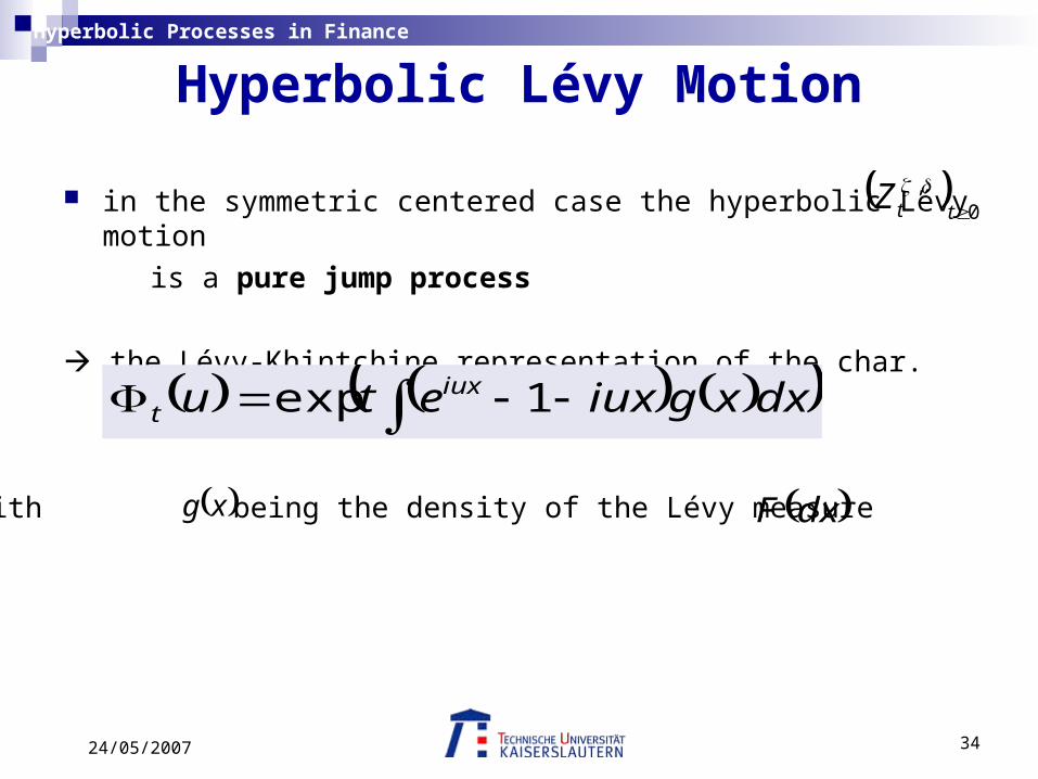
in the symmetric centered case the hyperbolic Lévy motion
is a pure jump process
the Lévy-Khintchine representation of the char. function is
Hyperbolic Lévy Motion
0,
ttZ
dxxgiuxetu iuxt 1exp
xg dxFwith being the density of the Lévy measure

3524/05/2007
Hyperbolic Processes in Finance
Hyperbolic Lévy MotionDensity of the Lévy measure:
1J
x
xdy
yYyJy
yx
xxgxg
exp
22
2exp1
,;0
21
21
2
2
• and are Bessel functions• using the asymptotic relations about Bessel functions, one can deduce that behaves like 1 / at the origin (x 0)
1Y
xg 2x
- Lévy measure is infinite, - hyp. Lévy motion has infinite variation,- every path has infinitely many small jumps in every finite time-interval

3624/05/2007
Hyperbolic Processes in Finance
The infinite Lévy measure is appropriate to model the everyday movement of ordinary quoted stocks under the market pressure of many agents.
The hyperbolic process is a purely discontinuous process but there exists a càdlag modification (again a Lévy process) which is always used.
The sample paths of the process are almost surely
continuous from the right and have limits from the left.
Hyperbolic Lévy Motion

3724/05/2007
Hyperbolic Processes in Finance
Hyperbolic Model of the Financial Market
rtBB
dtBrdB
B
t
ttt
tt
exp0
0
0ttr
0ttY
price process of a risk-free bond
interest rate process
tttt dZYdtbYdY 0ttZ
sZ
tsstt eZtZYY
0
0 1exp
price process of a stock
hyperbolic Lévy motion

3824/05/2007
Hyperbolic Processes in Finance
to pass from prices to returns: take logarithm of the price process
Hyperbolic Model of the Financial Market
sts
s
t
t
ZZ
tZ
Y
0
1log
log
results in two terms:
hyperbolic term
sum-of-jumps term
after approximation to first order the remaining term is
since Lévy measure is infinite and there are infinitely many small jumps, the small jumps predominate in this term; squared, they become even smaller and are negligible
2
tso
sZ
the sum-of-jumps term can be neglected and to a firstapproximation we get hyperbolic returns
3924/05/2007
Hyperbolic Processes in Finance
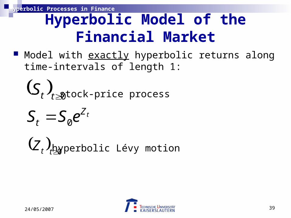
Model with exactly hyperbolic returns along time-intervals of length 1:
Hyperbolic Model of the Financial Market
tZ
t
tt
eSS
S
0
0
stock-price process
0ttZ hyperbolic Lévy motion

4024/05/2007
Hyperbolic Processes in Finance
Equivalent Martingale Measure
Definition:
An equivalent martingale measure is a probability measure Q, equivalent to P such that the discounted price process
is a martingale w.r.t. to Q.
Complication in the Hyperbolic model:
financial market is incomplete
no unique equivalent martingale measure (infinite number of e.m.m.) we have to choose an appropriate e.m.m. for pricing purposes
0
0
tt
rt
tt
t SeB
S

4124/05/2007
Hyperbolic Processes in Finance
Two approaches to find a suitable e.m.m.:
1) minimal-martingale measure
2) risk-neutral Esscher measure
In the Hyperbolic model the focus is on the risk-neutral Esscher measure. It is found with the help of Esscher transforms.
Equivalent Martingale Measure

4224/05/2007
Hyperbolic Processes in Finance
Esscher transforms:
The general idea is to define equivalent measures via
Equivalent Martingale Measure
1log
,exp0 0
Z
t t
sssF
eE
dsdZdP
dP
t
choose to satisfy the required martingale conditions
The measure P encapsulates information about market behavior;pricing by Esscher transforms amounts to choosing the e.m.m. which is closest to P in terms of information content.
* s

4324/05/2007
Hyperbolic Processes in Finance
In the hyperbolic model:
Equivalent Martingale Measure
tZt eSS 0
tZeEtM ,moment generating function of the hyperbolic Lévy motion 0ttZ
• The Esscher transforms are defined by
01, ttZ
t MeL t
• The equiv. mart. measures are defined via tF
LdP
dP
t
is called the Esscher measure of parameterP
4424/05/2007
Hyperbolic Processes in Finance
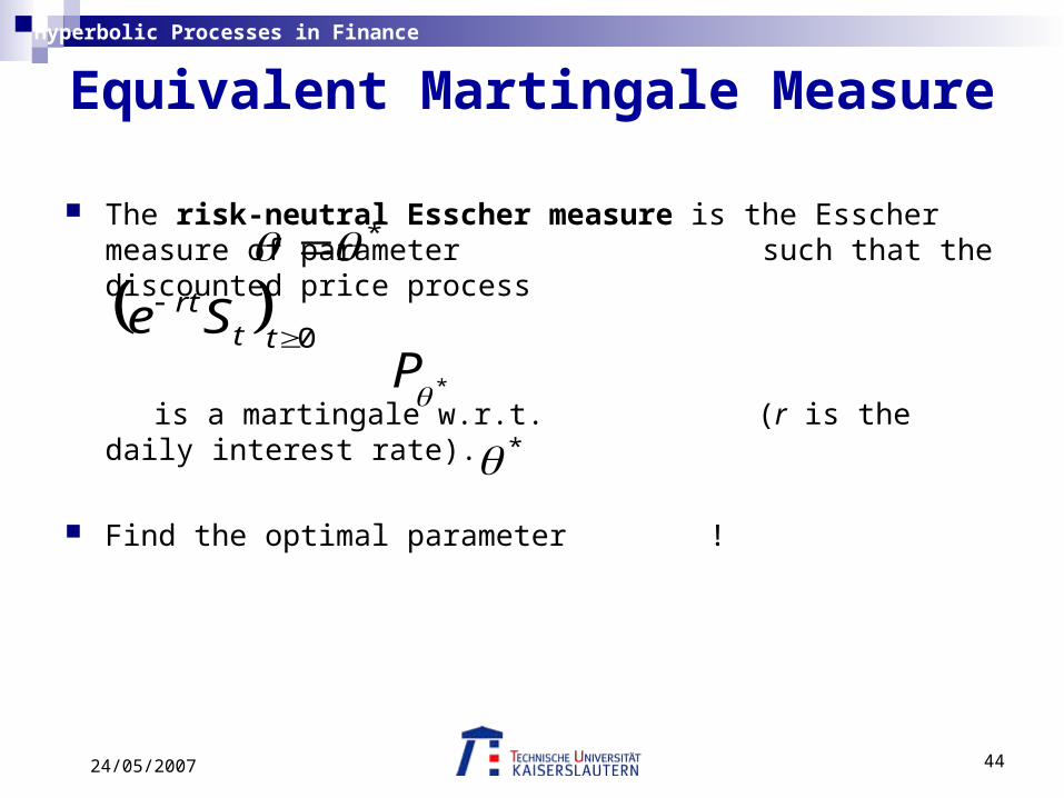
The risk-neutral Esscher measure is the Esscher measure of parameter such that the discounted price process
is a martingale w.r.t. (r is the daily interest rate).
Find the optimal parameter !
Equivalent Martingale Measure
*
0
ttrtSe
*P
*

4524/05/2007
Hyperbolic Processes in Finance
If is the density corresponding to the hyp. process,
define a new density via
Equivalent Martingale Measure
xht 0ttZ
dyyhe
xhexh
ty
tx
t
;
Density corresponding to the distribution of under the Esscher measure
0ttZP

4624/05/2007
Hyperbolic Processes in Finance
To find consider the martingale condition:
(expectation w.r.t. the Esscher measure )
This leads to:
The moment generating function can be computed as
Equivalent Martingale Measure
* 0
!*; SSeE t
rt *
P
reM
M
1,
1,1*
*
u
u
uK
KuM ,1,
222
2221
1
4724/05/2007
Hyperbolic Processes in Finance
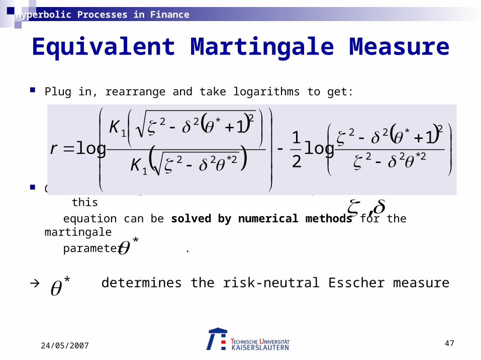
Plug in, rearrange and take logarithms to get:
Given the daily interest rate r and the parameters this
equation can be solved by numerical methods for the martingale
parameter .
determines the risk-neutral Esscher measure
Equivalent Martingale Measure
2*22
2*22
2*221
2*221 1
log2
11
log
K
Kr
,
**

4824/05/2007
Hyperbolic Processes in Finance
Option Pricing in the Hyperbolic ModelPricing a European call with maturity T and strike K ,
using the risk-neutral Esscher measure:
A usefull tool will be the Factorization formula:
Let g be a measurable function and h, k and t be real numbers, then
hkSgEhSEhSgSE tktt
kt ;;;

4924/05/2007
Hyperbolic Processes in Finance
Option Pricing in the Hyperbolic Model By the risk-neutral valuation principle (using the risk-neutral Esscher
measure) we have to calculate the following expectation:
*; KSeE TrT
**0 ;1; KSKPeKSPS T
rTT
Pricing-Formula for a European callwith strike K and maturity T
010 dS tdKe rT2
5024/05/2007
Hyperbolic Processes in Finance
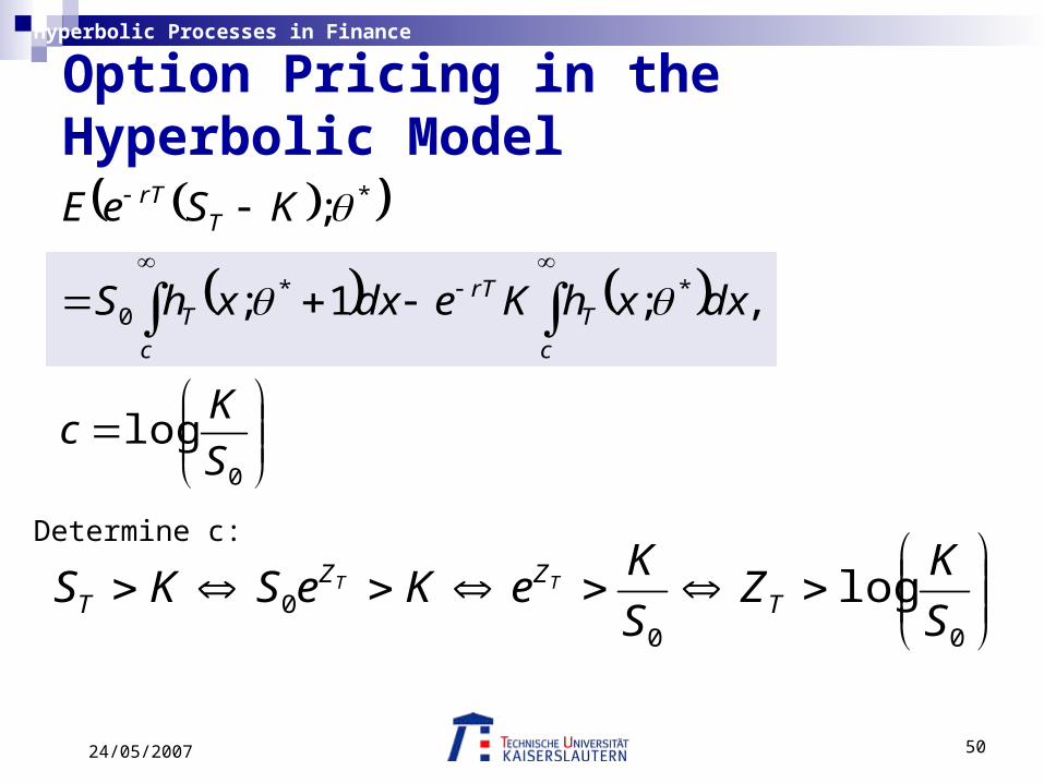
0
**0
*
log
,;1;
;
S
Kc
dxxhKedxxhS
KSeE
c
TrT
c
T
TrT
Option Pricing in the Hyperbolic Model
000 log
S
KZ
S
KeKeSKS TZZ
TTT
Determine c:
5124/05/2007
Hyperbolic Processes in Finance
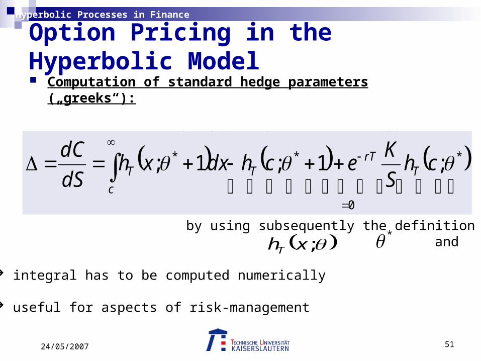
Computation of standard hedge parameters („greeks“):
E.g. compute the delta of a European call C:
Option Pricing in the Hyperbolic Model
0
*** ;1;1;
chS
Kechdxxh
dS
dCT
rTT
c
T
by using subsequently the definition of and ;xhT
* integral has to be computed numerically
useful for aspects of risk-management
5224/05/2007
Hyperbolic Processes in Finance
E./K. performed the same statistical analysis for the hyperbolic model as for the Black-Scholes model (to fit empirical data)
E.g. consider again the QQ-plots and density plots: Fig. 8, E./K., p.16 BASF Fig. 9, E./K., p.17 Deutsche Bank
Fit of the Hyperbolic Model to Empirical Data

5324/05/2007
Hyperbolic Processes in Finance
Fit of the Hyperbolic Model to Empirical Data

5424/05/2007
Hyperbolic Processes in Finance
Fit of the Hyperbolic Model to Empirical Data

5524/05/2007
Hyperbolic Processes in Finance
Fit of the Hyperbolic Model to Empirical Data

5624/05/2007
Hyperbolic Processes in Finance
Fit of the Hyperbolic Model to Empirical Data

5724/05/2007
Hyperbolic Processes in Finance
QQ-plots: almost no deviation from straight line;
assumption of hyperbolic distribution is supported
density plots: hyperbolic distribution provides an almost excellent fit
to the empirical data, esp. at the center and tails
Fit of the Hyperbolic Model to Empirical Data
The hyperbolic distribution fits empirical data better than the normal distribution.

5824/05/2007
Hyperbolic Processes in Finance
B./K. performed a similar study:
- daily BMW returns during Sep 1992 – Jul 1996 (100 data points)
- standard estimates for mean and variance of normal distribution
- computer program to estimate parameters of the hyp. distr.
maximum likelihood estimates:
Fig. 2, B./K., p.14 Density plots
Fit of the Hyperbolic Model to Empirical Data
^^^^
,,,
Comparison of option prices obtained from the Black-Scholes model and the hyperbolic model with real market prices shows, that the hyperbolic model provides a better fit.

5924/05/2007
Hyperbolic Processes in Finance
Fit of the Hyperbolic Model to Empirical Data
6024/05/2007
Hyperbolic Processes in Finance
Conclusion
The hyperbolic distribution provides a good fit for a range of financial data, not only in the tails but throughout the distribution
more accurate model for stock prices / returns
The hyperbolic model should esp. be preferred over the classical Black-Scholes model, when modeling daily stock returns, i.e. when looking at time periods of a single day.
6124/05/2007
Hyperbolic Processes in Finance
For longer time periods the Black-Scholes model is still appropriate:
E./K. estimated the parameters of the hyperbolic distr.
(2nd param.) for the stock returns of Commerzbank, considering
different time periods, i.e. 1, 4, 7, ……., 22 trading days
Conclusion
,

6224/05/2007
Hyperbolic Processes in Finance
Conclusion
^
^
^
the pairs ( , ) are given in the shape triangle and one can see, that the parameters tend to the normal distribution limit as the number of trading days increases
Fig. 7, E./K., p.15
Normal DistributionLimit

6324/05/2007
Hyperbolic Processes in Finance
References Bingham, Kiesel (2001): Modelling asset returns with hyperbolic distributions. In "Return Distributions in Finance", Butterworth- Heinemann, p. 1-20
Eberlein, Keller (1995): Hyperbolic distributions in finance. Bernoulli 1, p. 281-299
Barndorff-Nielsen, Halgreen (1977): Infinite divisibility of the hyperbolic and generalized inverse Gaussian distributions. Wahrscheinlichkeitstheorie und verwandte Gebiete 38, p. 309-311
Hélyette Geman: Pure jump Lévy processes for asset price modelling. Journal of Banking & Finance 26, p. 1297-1316

6424/05/2007
Hyperbolic Processes in Finance
Thank you for participating!