24-21 demografi

8/7/2019 24-21 demografi

http://slidepdf.com/reader/full/24-21-demografi 1/32

Demographic Research a free, expedited, online journal

of peer-reviewed research and commentary

in the population sciences published by the

Max Planck Institute for Demographic ResearchKonrad-Zuse Str. 1, D-18057 Rostock · GERMANY

www.demographic-research.org

DEMOGRAPHIC RESEARCH

VOLUME 24, ARTICLE 21, PAGES 497-526PUBLISHED 22 MARCH 2011http://www.demographic-research.org/Volumes/Vol24/21/

DOI: 10.4054/DemRes.2011.24.21

Research Article

Variance in death and its implications for

modeling and forecasting mortality

Shripad Tuljapurkar

Ryan D. Edwards

c 2011 Shripad Tuljapurkar & Ryan D. Edwards.

This open-access work is published under the terms of the Creative

Commons Attribution NonCommercial License 2.0 Germany, which permits

use, reproduction & distribution in any medium for non-commercial

purposes, provided the original author(s) and source are given credit.

See http://creativecommons.org/licenses/by-nc/2.0/de/

8/7/2019 24-21 demografi


Table of Contents

1 Introduction 498

2 Distributions of age at death over time, space, and characteristic 500

3 Theoretical models of adult mortality 505

3.1 General mortality model 505

3.2 The Gompertz model 506

3.3 The logistic model 506

3.4 General mortality, multiplicative frailty 507

3.5 General mortality, gamma multiplicative frailty 508

3.6 Gompertz mortality, gamma multiplicative frailty 508

3.7 Summary 509

4 Models of adult mortality in practice 510

4.1 Aggregate forecasting models 510

4.1.1 Mortality translation: Bongaarts-Feeney 5104.1.2 Generalized Gompertz: Lee-Carter 511

4.1.3 Implications 512

4.2 Short panel models 513

4.2.1 Cox proportional hazards 513

4.2.2 Accelerated failure time models 514

4.2.3 Kaplan-Meier estimation 515

4.2.4 Implications 515

5 Summary and discussion 516

6 Acknowledgements 517

References 518

A Mathematical appendix 522

A.1 General mortality model 522

A.2 The Gompertz model 523

A.3 The logistic model 523

A.4 General mortality, multiplicative frailty 524

A.5 General mortality, gamma multiplicative frailty 524

A.6 Gompertz mortality, gamma multiplicative frailty 525

8/7/2019 24-21 demografi


Demographic Research: Volume 24, Article 21

Research Article

Variance in death and its implications

for modeling and forecasting mortality

Shripad Tuljapurkar 1

Ryan D. Edwards 2

Abstract

The slope and curvature of the survivorship function reflect the considerable amount of

variance in length of life found in any human population. This is due in part to the well-

known variation in life expectancy between groups: large differences in race, sex, socioe-conomic status, or other covariates. But within-group variance is large even in narrowly

defined groups, and changes substantially and inversely with the group average length of

life. We show that variance in length of life is inversely related to the Gompertz slope

of log mortality through age, and we reveal its relationship to variance in a multiplicative

frailty index. Our findings bear a variety of implications for modeling and forecasting

mortality. In particular, we examine how the assumption of proportional hazards fails

to account adequately for differences in subgroup variance, and we discuss how several

common forecasting models treat the variance in the temporal dimension.

1 Morrison Professor of Population Studies, Department of Biological Sciences, Stanford University, Herrin

Labs 454, Stanford, CA 94305-5020. E-mail: [email protected] Corresponding author. Assistant Professor of Economics, Queens College and the Graduate Center, City

University of New York, and the National Bureau of Economic Research. Powdermaker 300-S, 65-30 Kissena

Blvd., Flushing, NY 11367. E-mail: [email protected]

http://www.demographic-research.org 497

8/7/2019 24-21 demografi


Tuljapurkar & Edwards: Variance in death and its implications for modeling and forecasting mortality

1. Introduction

Length of life is a fundamental dimension of human prosperity. We measure this di-

mension either with period life expectancy at birth, e0, the average length of life, or we

measure its inverse either with age-specific mortality rates that underpin the life table, or

with the log odds of death. Correctly modeling mortality is crucial for inference in both

observational and experimental settings, and thus for forecasting. In this paper, we illus-

trate how patterns in the variance of length of life, whether measured across subgroups at

a point in time or in human populations over long periods of time, bear strong implica-

tions for how we model mortality and test hypotheses in cross-sectional and longitudinal

settings.

In the cross section and over short panels, the Cox (1972) proportional hazards model

and the logit or logistic regression model are standard tools in epidemiological studies

and in medical research. As they are typically specified, these models assume that sub-

groups experience proportionally higher or lower hazards relative to a baseline. We show

that cross-sectional patterns in the variance in length of life across subgroups, where vari-

ance is inversely related to average life expectancy, are not at all adequately captured by

proportional hazards. This is because variance in length of life is closely tied to the age

slope of mortality; subgroup differences in the variance in length of life are equivalent

to subgroup differences in the age slope of mortality. Regardless of the precise nature of

baseline mortality, which may be modeled nonparametrically, proportional hazards im-

pose the same age slope and thus the same variance in length of life on all subgroups.

Violations of the proportional hazards assumption have been extensively remarked

and explored (Hess, 1995; Lee and Go, 1997; Therneau and Grambsch, 2000), and re-searchers have suggested various methods to address them. One option is to augment stan-

dard models by injecting individual frailty (Vaupel, Manton, and Stallard, 1979; Hougaard,

1995). As we discuss, frailty models are helpful because they add an additional param-

eter that makes a direct impact upon variance. But the concept of frailty does not help

us intuitively understand cross-sectional or intertemporal patterns in variance; it simply

improves the fit of models without increasing our understanding. One class of models de-

signed to account for frailty, accelerated failure time (AFT) models, posits a proportional

scaling of the distribution of survival time across subgroups, which inappropriately im-

plies a positive rather than negative relationship between mean and variance. Approaches

that relax the assumption of proportional scaling, such as the use of stratified Cox re-gression, time-dependent covariates, or the nonparametric method of Kaplan and Meier

(1958) are preferable.

From an aggregate perspective, the expansion of human life in the past century (Pre-

ston, 1975; Caldwell, 1976) and its socioeconomic implications have stimulated efforts

to analyze and forecast mortality trends (Tuljapurkar and Boe, 1998), which are guided

498 http://www.demographic-research.org

8/7/2019 24-21 demografi



by insights gained from mortality models. A natural focus of these efforts is the period

expectation of life at birth, e0. Mortality change is commonly summarized in terms of

trends in e0, and mortality models are evaluated on their ability to match historical trends

in life expectancy. These uses of e0 gained considerable support from two recent findings:

that e0 has increased at a nearly constant rate in many industrial countries since 1955

(White, 2002), and that since 1840 annual world record female e0 has also increased at a

nearly constant rate (Oeppen and Vaupel, 2002). Some have argued that such constancy

is fundamental in analyzing mortality change (Bongaarts and Feeney, 2002, 2003), and

one researcher (Bongaarts, 2005) has extended a simple model (Vaupel, 1986) to forecast

mortality change. But e0 is only the mean of the distribution of ages at death, and we show

here that the variance of this distribution provides important additional information. As

we reveal, temporal change in the variance in age at adult death is not necessarily captured

by simple models, which may inappropriately constrain how we should conceptualize and

analyze mortality change.

This paper is organized in four main parts. First, we discuss cross-sectional and tem-

poral patterns in distributions of period life-table ages at death. We recount how historical

increases in e0 in the industrialized countries have been accompanied by equally strik-

ing decreases in the variance of the age of adult death (Edwards and Tuljapurkar, 2005).

These trends show clearly that mortality decline over time has compressed the variance

between individuals at the same time as it has increased average life expectancy. Cross-

sectional patterns reveal the same inverse relationship between subgroup variance and

average. While overall variance has declined over time, very large differences in vari-

ance between subgroups remain. Less advantaged groups experience both lower average

length of life and higher variance.Second, we show how the variance in age of adult death can be approximately com-

puted for any reasonable model of mortality rates, and illustrate this with three commonly

used models, the Gompertz (1825), the logistic, and a Gompertz model with multiplica-

tive frailty. In particular, we reveal the inverse relationship between the Gompertz slope

and the variance in length of adult life. A particular age slope of mortality will reflect a

particular variance, but while it can be consistent with different subgroup average lengths

of life, it cannot accurately capture the large differences in subgroup variances. Adding

frailty into the model can explain variance, but not in a satisfactory way in terms of any

intuition.

Third, we explore the implications of these insights for common mortality models. Asconcerns forecasting, we show that any generalization of the Bongaarts-Vaupel translation

argument yields an unchanging variance in the age at adult death over time, which may or

may not be a preferable characteristic. Over long periods of time, trends in variance have

comprised a major qualitative aspect of mortality change in industrialized countries, and

we suspect the same is true for developing countries. We recount world-record trends in


8/7/2019 24-21 demografi



the variance in age of adult death, and discuss their implications for understanding secular

mortality change. In the setting of panel data on individuals, we illustrate how Gompertz

slopes that vary systematically across subgroups violate the assumption of proportionality,

and we discuss how various methods to address this either succeed or fail in modeling

variance correctly.

Finally, we discuss how our results fit into ongoing research on aging more generally.

Insights into the plasticity of the Gompertz slope and what may be driving it are particu-

larly relevant for gauging the future of the human aging process. Results in the literature

on genetic interventions in nonhuman species become particularly intriguing when com-

bined with the insights we present here. Our results are related to work on the “rectan-

gularization” of the survivorship schedule (Wilmoth and Horiuchi, 1999; Kannisto, 2000)

and on its shape more generally (Cheung et al., 2005). They are also connected to research

on the existence of a maximum age at death (Fries, 1990; Olshansky, Carnes, and Cassel,

1990; Wachter and Finch, 1997). All these topics subsume questions as to the possible

limiting forms of the distribution of age at death. Our analysis makes no assumptions or

deductions about such a limit, but aims to illuminate the nature and significance of trends

in the variability of age at death.

Other recent work in social science examines contributions of subgroup variance to

overall inequality in other measures of well-being such as income (Western and Bloom,

2009). We believe such research shows much promise, and that applying similar tech-

niques to the study of mortality would prove fruitful in future pursuits. Our focus here

is primarily on aggregate inequality in length of life, which we show is linked to the

Gompertz slope and the commonly used proportional hazards model.

2. Distributions of age at death over time, space, and characteristic

The age pattern of life table deaths in any period, which is also the distribution of period

length of life, is found from mortality rates µ(a) by age a in that period. We define

cumulative mortality as

M (a) =

a

0

µ(s) ds, (1)

and survivorship is given by

(a) = exp

−

a

0

µ(s) ds

= (a) = exp[−M (a)]. (2)

The probability density of death at age a is

φ(a) = µ(a) (a). (3)


8/7/2019 24-21 demografi



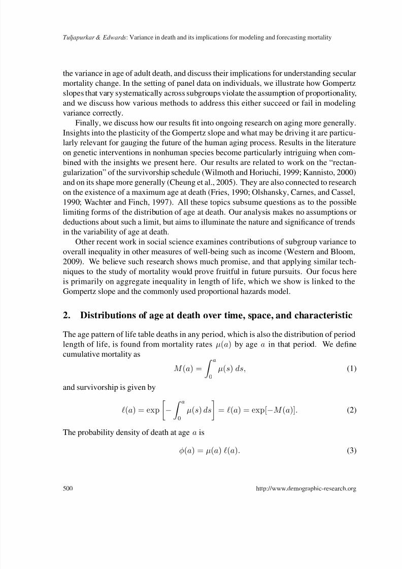
Even when it is small as in industrialized countries during the past half century, infant

mortality produces some nonzero φ(0) at the extreme left end of the distribution. But

φ(a) falls to very low levels thereafter and remains low until well into adult ages.

Figure 1 plots φ(a) for racial subgroups within the U.S. in 2004 based on life tables

prepared by Arias (2007). In that year, e0 among African Americans was 73.1 years, 5.2

fewer years than for whites. Part of this was due to a greater density of deaths in infancy,

which approached 0.015% for blacks, more than twice the level for whites, but there were

also differences in the much larger probability of death at older ages. Life expectancy

conditional on reaching age 10, e10, was 68.9 for whites but only 64.3 for blacks. The

width of the distribution around older ages, which we measure by the standard deviation

above age 10 or S10, introduced by Edwards and Tuljapurkar (2005) and discussed shortly,

is also visibly different across racial groups. For whites in 2004, S10 = 14.9, while among

blacks it was almost 2 years higher. Patterns of inequality in length of life through other

dimensions of socioeconomic status (SES) such as income or education look essentially

the same (Edwards and Tuljapurkar, 2005), as do differences by sex.

Figure 1: Distributions of age at death by race in the U.S. in 2004

0 10 20 30 40 50 60 70 80 90 1000

0.005

0.01

0.015

0.02

0.025

0.03

0.035

0.04

0.045

Age

Density

White S10

= 14.9

Black S10

= 16.7

Whites in 2004

African Americans in 2004

Source: Arias (2007). Data are life-table deaths by race ndx for both sexes combined.


8/7/2019 24-21 demografi



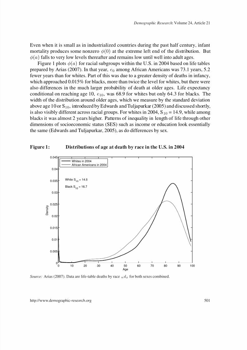
A similar picture emerges when we examine distributions of length of life over time

instead of across characteristic. Figure 2 plots deaths for both sexes combined in Swe-

den in 1900 and 2000, revealing that long-term temporal variation looks a lot like cross-

sectional variation. Higher status or more time is rewarded with less variance and higher

mean. Dissimilarities include the much higher level of infant mortality in 1900 and the

large “baseline” probability of death at practically any age. Both of these features re-

flected the prevalence of infectious disease before the completion of the epidemiological

transition.

Figure 2: Distributions of age at death in Sweden in 1900 and 2000

0 10 20 30 40 50 60 70 80 90 1000

0.005

0.01

0.015

0.02

0.025

0.03

0.035

0.04

0.045

Age

Dens

ity

2000 S10

= 12.9

1900 S10

= 20.7

Sweden in 2000

Sweden in 1900

Source: Human Mortality Database (2009). Data are life-table deaths ndx for both sexes combined.


8/7/2019 24-21 demografi



Comparing Figures 1 and 2 reveals another interesting pattern of differences in the

distribution of length of life across geographic boundaries. The standard deviation in

adult length of life among U.S. whites, is about 2 years higher than it is in Sweden. This

is the point made by Wilmoth and Horiuchi (1999) and Edwards and Tuljapurkar (2005),

and recently extended to developing countries by Edwards (2010). Cross-national trends

conform to the pattern of higher status bringing higher mean and lower variance.

We measure variance in adult ages at death by choosing a cutoff age A at which prob-

abilities of death are near their minimum and are relatively stable over time. Following

Edwards and Tuljapurkar (2005), we focus on S10, the standard deviation of length of life

starting from age A = 10, but results are similar across various cutoffs. Infant and child

deaths contribute strongly to total variation in length of life, but as we now explain, they

do so in a relatively uninformative way that masks important trends. Consider the average

age at death starting from birth in the period life table, also known as e0. Write T for

the random age of death of an individual in a hypothetical cohort following a period life

table, where (A), the familiar survivorship probability at age A, is also the probability

of adult death (T > A). Then period life expectancy at birth can be decomposed as

e0 = [1 − (A)] M − + (A) M +, (4)

where M − and M + are (conditional) average ages of death for those who die young or

die as adults, respectively. In the industrialized countries in the last five or six decades,

M − is much below 1 year for all subgroups, and 1− (A) is well under 10%, so the main

determinant of e0 is the timing of adult death. We can also decompose total variance

starting from birth as

Var(T ) = [1− (A)] V − + (A) V + + [1− (A)] (M − − e0)2 + (A) (M + − e0)2, (5)

where V − and V + are (conditional) variances of age at death for those who die young or

die as adults. For all subgroups in the industrialized countries, only the second and third

of these four terms matter. The first term is small because both its components are small,

and the last term is small because e0 has become almost arbitrarily close to M +. While

the third term contributes substantially to Var(T ), it does so only because M − is very

small relative to e0. This difference is not at all informative about substantive variation in

the adult ages at which most deaths occur.

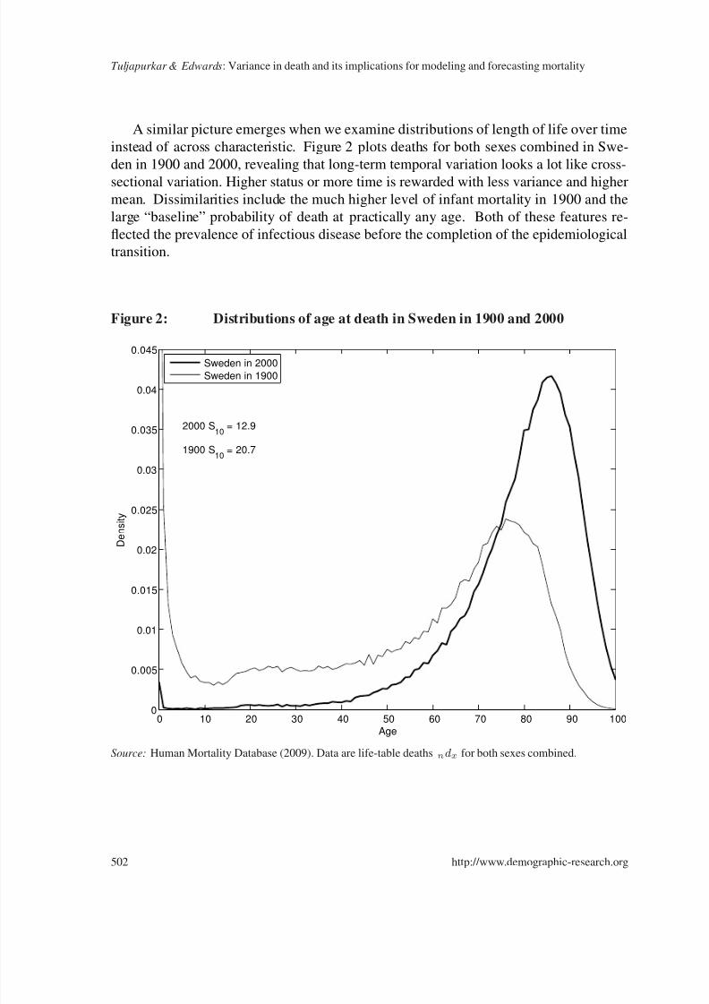
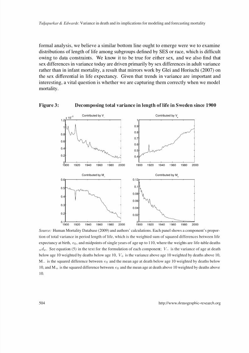
Figure 3 shows the four components in equation (5) using Swedish data over theperiod 1900 to 2003 and A = 10. Since about 1940, the element that matters most to

understanding total variability in age at death is the second term in equation (5), (A) V +,

which is shown at upper right. Today, variance in length of life above age 10 accounts for

over 85% of total variability in Sweden, while variance below age 10 such as attributable

to infant mortality is responsible for less than 15%. While we have not performed a


8/7/2019 24-21 demografi



formal analysis, we believe a similar bottom line ought to emerge were we to examine

distributions of length of life among subgroups defined by SES or race, which is difficult

owing to data constraints. We know it to be true for either sex, and we also find that

sex differences in variance today are driven primarily by sex differences in adult variance

rather than in infant mortality, a result that mirrors work by Glei and Horiuchi (2007) on

the sex differential in life expectancy. Given that trends in variance are important and

interesting, a vital question is whether we are capturing them correctly when we model

mortality.

Figure 3: Decomposing total variance in length of life in Sweden since 1900

1900 1920 1940 1960 1980 20000

0.2

0.4

0.6

0.8

1

1.2x 10

−3 Contributed by V−

1900 1920 1940 1960 1980 2000

0.4

0.5

0.6

0.7

0.8

0.9

1

Contributed by V+

1900 1920 1940 1960 1980 20000.1

0.2

0.3

0.4

0.5

0.6

Contributed by M−

1900 1920 1940 1960 1980 20000

0.02

0.04

0.06

0.08

0.1

0.12

Contributed by M+

Source: Human Mortality Database (2009) and authors’ calculations. Each panel shows a component’s propor-

tion of total variance in period length of life, which is the weighted sum of squared differences between life

expectancy at birth, e0, and midpoints of single years of age up to 110, where the weights are life-table deaths

ndx. See equation (5) in the text for the formulation of each component; V − is the variance of age at death

below age 10 weighted by deaths below age 10, V + is the variance above age 10 weighted by deaths above 10,

M−

is the squared difference between e0 and the mean age at death below age 10 weighted by deaths below

10, and M+ is the squared difference between e0 and the mean age at death above 10 weighted by deaths above

10.


8/7/2019 24-21 demografi



3. Theoretical models of adult mortality

The most celebrated model of adult age-specific mortality is that of Gompertz (1825), in

which the force of mortality rises exponentially with age. But recent work by Vaupel et al.

(1998), Thatcher, Kannisto, and Vaupel (1998) and others suggests that a logistic model

with an asymptote describes old-age mortality more accurately. The logistic can also be

seen as a result of a model in which Gompertz mortality is modified by a multiplicative

frailty (Vaupel, Manton, and Stallard, 1979). Frailty, if it occurs in this form, should

clearly contribute to the variability in age at death. While it can, we do not find this

an entirely compelling account of historical or cross-sectional patterns in S10. Overall,

traditional models are not well-equipped to deal with or provide understanding about

variance.

We next present analytical results showing how the variance in age at adult death

depends on the parameters of mortality models. We consider first a general mortalitymodel without frailty, and the special cases of Gompertz and logistic, then a general

model with multiplicative frailty, with special cases of gamma frailty, and Gompertz with

gamma frailty.

3.1 General mortality model

Suppose that adult mortality µ(a) is an increasing positive function of age a. Survivor-

ship falls to zero as age increases because cumulative mortality M (a) is increasing. The

probability distribution of age at death for adults, φ(a), increases at young adult ages,

reaches a mode a0 and then falls, ultimately reaching zero by very high ages.

To proceed, we take a Taylor expansion of the age-at-death distribution φ(a) around

the mode a0, and then we approximate the resulting quadratic with a normal distribu-

tion. The mathematical appendix presents detailed steps. The end result is the following

relationship:

φ(a) ≈ φ(a0) exp

−

(a − a0)2

2 σ2

, (6)

where

σ2

=φ(a0)

|φ(a0)| =µ(a0)

|µ(a0) − 2 µ3(a0)| . (7)

The variance term σ2 depends on the curvature of the mortality function and roughly

equals the variance in age at adult death. This approximation provides a useful and often

accurate estimate of the moments of φ(a) — we use it here and also check its accuracy

by numerical computation.


8/7/2019 24-21 demografi



3.2 The Gompertz model

We write the Gompertz mortality function as

µ(a) = µ0 eβ a, (8)

where the parameter β is the familiar age-slope of log mortality, a constant in the Gom-

pertz model. In the U.S. for both sexes combined, the age-slope is about 0.087 (Edwards,

2009); that is, mortality rates increase 8.7% with each year of age. From equation (7) (see

appendix) the variance in adult age at death is approximately given by

σ2 ≈1

β 2. (9)

Thus the Gompertz variance in age at death depends only on the slope parameter β and noton µ0. It is possible to obtain an exact expression for the variance by analytical integration

in terms of special functions, but the results are not especially illuminating. However, we

have computed numerically the exact variance for a range of values of β and µ0 that

are appropriate for twentieth century human mortality. We find that the exact value of σdepends only weakly on µ0 and that equation (9) is a very accurate approximation.

It follows that a Gompertz model can only describe differences in the variance of the

adult age at death with differences in the Gompertz parameter β , the age-slope of log

mortality. There is a one-to-one inverse relationship between the age-slope of mortality

and the variance in length of life. Were equation (9) an exact relationship, β = 0.087

would be consistent with σ = 11.5.

3.3 The logistic model

When measured by S10, U.S. levels of σ are higher than implied by β = 0.087, more in

the range of 15.0 rather than 11.5. We know there are departures from linearity in log

mortality rates at advanced ages; how does this affect σ as a function of β ? We write the

logistic model for mortality as

µ(a) =eβ a

C + eβ a, (10)

where C is the asymptote, commonly set to equal unity. From equation (7) (see appendix)the approximate variance is

σ2 =1 + β

β 2. (11)

Thus the logistic also displays the remarkable property that the variance in age at death

depends only on the slope parameter β . It follows that a logistic model can only describe


8/7/2019 24-21 demografi



changes in the variance of the adult age at death if the slope parameter β changes with

time.

Note that if we fit a Gompertz model and a logistic model to a particular data set, the

value of β must be similar in both. To see why, compare the two models near a = 0 which

here indicates the start of adult age. With the same β , the logistic model implies only a

slightly larger variance in age at adult death than the Gompertz. We expect this difference

because the density φ for the logistic model shallows as age increases; see the discussion

after equation (6). For β = 0.087, equation (11) implies σ = 12.0, closer to reality than

the Gompertz but not by much. Of course, when we measure σ with S10, we are including

variance due to traffic accidents, violence, and other causes that asymmetrically make an

impact upon the young in a decidedly non-Gompertz way. For the U.S., this problem may

be particularly acute. Edwards and Tuljapurkar (2005) find that removing external-cause

mortality reduces S10 by 1–1.5 years, leaving still perhaps 1.5 years in extra S10 that

cannot be well explained by logistic or decelerating log mortality, or by external causes.

A natural next step is to examine the connection between frailty in mortality and

variance in length of life, two concepts that are related. A convenient way to proceed is

by generalizing the Gompertz model. Next we discuss a model that incorporates frailty,

including two special cases.

3.4 General mortality, multiplicative frailty

Following Vaupel, Manton, and Stallard (1979), suppose that every individual has a ran-

dom frailty Z and that g(z) dz is the probability that Z takes values between z and z +dz.

Then mortality µ̄ is given by the product of the frailty parameter Z and a baseline mortal-ity function µ(a):

µ̄(a|Z ) = Z µ(a). (12)

The usual specification of a frailty distribution assumes that average frailty is 1, and

that the distribution of frailty has some variance. It is convenient to define the following

averages with respect to frailty:

hj(a) = E [Z j e−Z M (a)], for j = 1, 2, 3. (13)

Then the approximate variance in age at death is just a generalization of equation (7):

σ2 =φ(a0)

|φ(a0)|=

h1(a0)µ(a0)

|φ(a0)|. (14)

As shown in the appendix, φ depends on h1, h2, and h3. But when every frailty is set

equal to 1, these are all equal, and the variance is reduced to the value in equation (7).


8/7/2019 24-21 demografi



3.5 General mortality, gamma multiplicative frailty

To obtain a useful qualitative sense of the effect of frailty, we consider the special case

when frailty Z follows a gamma distribution (Vaupel, Manton, and Stallard, 1979). Letthe probability that Z lies between w and w + dw be given by g(w) dw, where

g(w) =kk

Γ(k)wk−1 e−k. (15)

The average frailty is 1 and the variance of frailty is Var(Z ) ≡ s2 = 1/k.

As we show in the appendix, the magnitude of frailty selection depends on both the

variance in frailty s2 and the cumulative mortality hazard. Strong selection works to de-

crease the modal age at death. To examine the variance, we can find the second derivative

φ at the modal age and use it in a Taylor approximation:

σ2 =µ(a0)

|µ(a0) − µ3(a0) [(1 + s2)(2 + s2)] / [(1 + s2M (a0)2)] |. (16)

The selection effect appears in the denominator, where s2 multiplies by the cumulative

mortality M (a0) at ages below the mode. Strong selection via a large M (a0) will com-

bine with variance in frailty s2 to reduce the denominator and thus inflate the variance σ2

in age at death.

3.6 Gompertz mortality, gamma multiplicative frailty

We can learn more by combining the above multiplicative gamma-distributed frailty with

the Gompertz baseline mortality from equation (8). In the appendix, we derive the modal

age at death for such a model. We obtain the variance in age at death using equation (16),

equation (33) from the appendix, and a little algebra, which yields the parsimonious result

that

σ2 =(1 + s2)

β 2. (17)

Comparing this with equation (9) for the standard Gompertz, both shown along the bottom

row in Table 1, shows that frailty amplifies the variance in age at death. A Gompertz

model with gamma frailty can describe changes in the variance of the adult age at death

with changes either in the Gompertz slope parameter β , or in the variance in frailty s2, or

in both.


8/7/2019 24-21 demografi



Table 1: Characteristics of the distribution of adult death in three models

Parameter Gompertz Logistic Gompertz Gamma

Mortality at ageµ0e

βa eβa

C+eβaZµ0e

βa

a, µ(a)

Density of deathsµ(a)e−(µ(a)−µ0)/β (C + 1)1/β eβa

(C+eβa)1+1/β µ(a)

kk+M (a)

k+1at a, φ(a)

Mode age at 1β

log(β/µ0) 1β

log(βC ) 1β

log(β/µ0 − s2)death, a0

Variance in age 1β2

1+ββ2 1+s

2

β2at death, σ2

Notes: In the logistic model, C is the asymptote, commonly set to equal one. The cumulative force of mortality

at age a is M (a) = a0 ds µ(s). In the Gompertz Gamma model, the multiplicative frailty index Z is

distributed gamma with density equal to g(w) = kk

Γ(k)wk−1 e−k , an average E (Z ) = 1, and a variance

Var(Z ) ≡ s2 = 1/k.

3.7 Summary

Our key finding is that the Gompertz slope of log mortality through age, often called therate of aging, is inversely related to the variance in length of life. Differences across time,

space, or SES in the latter can only be captured by differences in age-slopes of mortality.

This insight is not greatly altered if mortality follows a logistic curve, flattening out at

advanced ages. Injecting frailty into standard mortality models loosens the relationship

between variance in life span and the Gompertz slope. A Gompertz model with Gamma

multiplicative frailty allows us to model heterogeneity in variance as deriving from het-

erogeneity in either the Gompertz slope, in the variance in frailty, or in both.

Normative or etiological insights from our exploration of these models are more elu-

sive. The basic result concerning variance in the Gompertz slope is important because

some have viewed the Gompertz slope as a kind of species-specific parameter that is eter-nally fixed while the intercept may fluctuate (Finch, Pike, and Witten, 1990). But we

show it can only be constant if we add a free parameter such as frailty and allow it to fluc-

tuate arbitrarily in order to fit the data. A more straightforward reading of the evidence

is that instead, both nature and nurture must affect the Gompertz slope, at least in human

populations and potentially in other species.


8/7/2019 24-21 demografi



The addition of multiplicative frailty to a Gompertz model only addresses changing

variances in age at death if we assume that frailty distributions have been changing quite

rapidly over time. Temporal change in frailty has not been a standard feature of mortality

models, and it is not clear why the distribution of such frailties would have narrowed.

From an evolutionary perspective, it is not clear why frailty should have persisted into

modern humans at all. It is also unclear why in the cross section African Americans

should have persistently higher frailty than whites, or why Americans in general should

endure higher levels than Europeans or Japanese. Frailty models may allow us to model

mortality better in a strictly mechanical sense, but they do not appreciably improve our

understanding.

4. Models of adult mortality in practice

These results concerning variance in length of life and the age-slope of mortality bear

implications for modeling and forecasting. In this section we examine how variance is

implicitly or explicitly treated in an array of common frameworks. We first examine fore-

casting models, including a recent technique that involves mortality “translation,” which

we explain below, as well as the the popular Lee and Carter (1992) forecasting model,

which can be seen as a generalized Gompertz model. Then we discuss several standard

mortality models that are commonly used in short panels with microdata, where cross-

sectional patterns in variance are more important. We examine the Cox (1972) model, the

class of nonparametric models suggested by the methods of Kaplan and Meier (1958), and

accelerated failure time (AFT) models, which some have associated with frailty models.

4.1 Aggregate forecasting models

4.1.1 Mortality translation: Bongaarts-Feeney

The pioneering model of mortality translation due to Bongaarts and Feeney (2003) pro-

vides an appealingly simple description of mortality change, although it is controversial.

A recent edited volume by Barbi, Bongaarts, and Vaupel (2008) provides a thorough

overview of the method, which is related to the concept of tempo effects in mortality

(Bongaarts and Feeney, 2002).

One can describe the Bongaarts-Feeney model in terms of a hypothetical cohort fol-lowing a period life table. Let T 1 be the random age at death of an individual in this cohort

in period t1. In a later period t2 > t1, suppose that the effect of mortality change between

the two periods is completely described by delaying each death by the same amount. We

assume infant mortality is practically zero and thus can also be delayed in this fashion,

which although unrealistic is consistent with our focus on adult mortality. Each random


8/7/2019 24-21 demografi



age at death T 1 in the first period is thus replaced in the later period by the random age

at death T 1 + D, where D > 0 is fixed. We see at once that the average age at death

increases from e0(t1) = E [T 1] in period t1 to e0(t2) = e0(t1) + D in the later period

t2. If we increase the mean age at death by some fixed annual amount, we have found a

model of mortality change that describes a constant trend in e0. We use the term mortality

translation for any such model.

Notice that translation only affects the mean age at death and not its variance. Shift-

ing every random age at death from T 1 to T 2 = T 1 + D results in a constant variance,

Var(T 1) = Var(T 2), so long as D is fixed. In fact, translation leaves unchanged all the

central moments of the random age at death. Put geometrically, translation necessarily

implies that the shape of the distribution of age death does not change.

Mortality translation is appealing because it can be used with any mortality model.

Bongaarts and Feeney (2003) and Bongaarts (2005) used translation for a Gompertz and

a logistic model. Vaupel (1986) used a Gompertz model in essentially the same way,

although he did not explicitly refer to translation.

It is obvious that mortality translation, by construction, cannot describe temporal

changes in the variance in the probability distribution of age at death, or for that matter,

of other central moments of φ related to the shape of the distribution, such as skewness

or kurtosis. As revealed by Wilmoth and Horiuchi (1999), Cheung et al. (2005), and

Edwards and Tuljapurkar (2005), trends in all of these moments have been and remain

very interesting even in industrialized countries. Prior to 1960, S10 was strongly declin-

ing in industrialized countries, a pattern that is repeating itself among many developing

countries today (Edwards, 2010). To be sure, Bongaarts and Feeney (2003) never in-

tended their model to apply universally across historical periods; their aim was mortalityforecasting for the U.S. and other industrialized countries. But while S10 has remained

roughly steady on average in the U.S. since 1960, it has also fluctuated up and down

within a 1.5-year band over time (Edwards and Tuljapurkar, 2005), or ±5%. Forecasting

via translation makes a strong prediction about long-term trends in the variance.

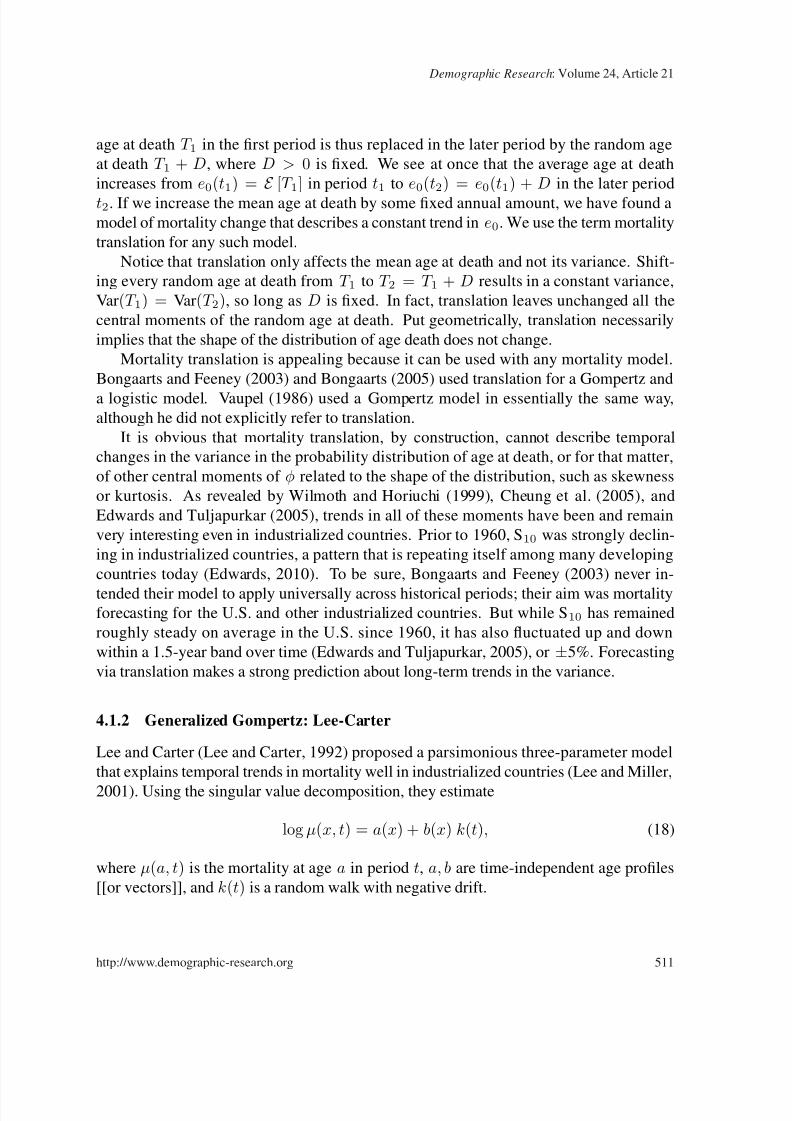
4.1.2 Generalized Gompertz: Lee-Carter

Lee and Carter (Lee and Carter, 1992) proposed a parsimonious three-parameter model

that explains temporal trends in mortality well in industrialized countries (Lee and Miller,

2001). Using the singular value decomposition, they estimate

log µ(x, t) = a(x) + b(x) k(t), (18)

where µ(a, t) is the mortality at age a in period t, a, b are time-independent age profiles

[[or vectors]], and k(t) is a random walk with negative drift.


8/7/2019 24-21 demografi



The profile a(x) is an average of age-specific log mortality rates over the historical

sample period, so it ends up being approximately Gompertz or logistic in shape. But b(x)is not necessarily constant with age, as it would have to be in a Gompertz model with

a fixed age slope over time. Indeed, fits of b(x) typically reveal stark age differences in

rates of mortality decline in industrialized countries (Tuljapurkar, Li, and Boe, 2000). By

consequence, the slope and curvature of mortality in this model are free to evolve over

time, which as our results show can easily lead to changes in the variance of age at death.

The singular value decomposition of equation (18) produces optimal fits of age-specific

mortality rates; the moments of the distribution of ages at death are backed out of the

model rather than hard-wired as in the Bongaarts-Feeney translation model.

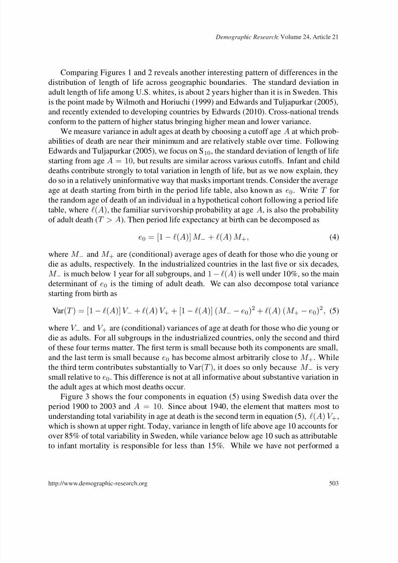
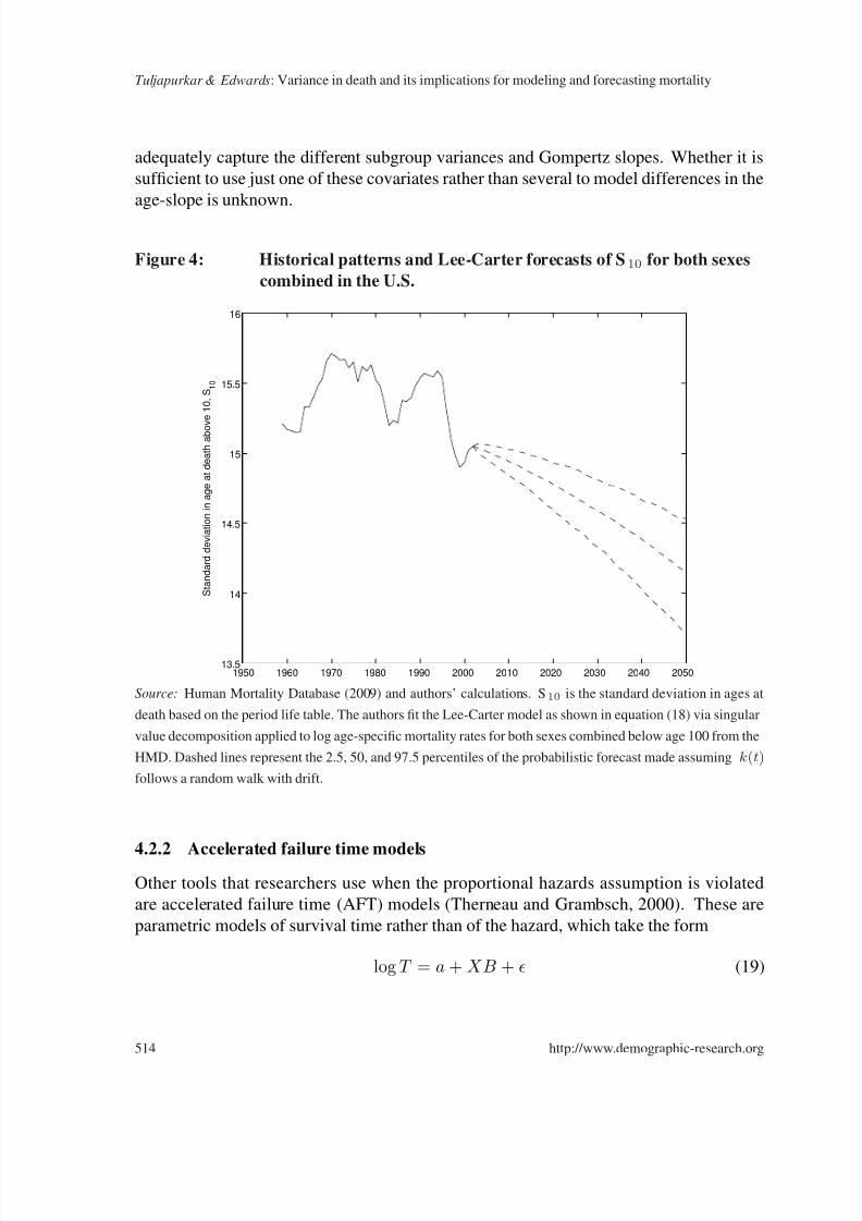
Figure 4 depicts historical data since 1959 and probabilistic forecasts of S10 for U.S.

out to 2050 using the Lee-Carter model applied to log mortality rates for both sexes com-

bined from the Human Mortality Database (2009). The forecast is shown by three dashed

lines that indicate the 2.5, 50, and 97.5 percentiles of the distribution. Several charac-

teristics are informative. There is clearly a trend in S10, which declines in the median

forecast from 15 years around 2000 to just above 14 years by 2050. While this looks

like a bold prediction given the figure, by comparison practically all other high-income

countries except for France already enjoy levels of S10 around 14 or below.

4.1.3 Implications

Over the last two centuries, the variance in age at adult death as measured by the standard

deviation S10 has declined by almost 50%. Were we to use a Gompertz model to describe

period mortality at ages over 10, then the slope of the Gompertz model would have toincrease by about 40% in order to replicate observed trends in S10. A logistic model for

period mortality would require a larger increase, about 50%, in the slope. Over the past

50 years, the trend in S10 has been toward much more gradual decline, perhaps 1% in the

U.S., but temporary fluctuations in the variance around its slight downward trend have

been much larger, more like 10%.

Because mortality translation models do not allow for any change in the variance of

adult death, we urge some caution in applying their results to the age pattern of deaths,

even though they may describe recent changes in e0 perfectly well. A striking result

about long run mortality change is the demonstration by Oeppen and Vaupel (2002) that

world-record high e0 has risen at a remarkable linear rate over the past 160 years. Suchuniformity suggests that upper bounds on life span, prognosticated and then consistently

broken throughout this period, are not as clear as some currently believe. The pace of hu-

man development and achievement measured in this way has been rapid and surprisingly

steady across several distinct periods of socioeconomic and epidemiological transitions.

But Edwards and Tuljapurkar (2005) describe how long-term trends in the record-low


8/7/2019 24-21 demografi



variance paint a very different picture regarding the gains in human well-being along

the dimension of mortality. True, progress against the Gompertz slope has indeed been

achieved, contrary to the opinions of those who may have viewed it as immutable. But

long-term gains have come more in fits and starts rather than continuously, and this high-

lights the remaining challenges, as does the considerable heterogeneity across countries in

progress against variance during the last century. We do not fully understand the sources

of variance in life spans, nor the underlying health inequalities they presumably reflect,

and this is a problem for policy as well as for modeling and forecasting mortality. Trans-

lation models provide a good statistical fit to mortality patterns in industrialized countries

since 1950 (Bongaarts, 2005). But the shape of the age distribution of deaths provides

enough important insights that we should probably not assume it to be fixed over long

periods of time. By contrast, the Lee and Carter (1992) forecasting model can and does

predict changes in the variance in the age at death, but with caveats.

4.2 Short panel models

4.2.1 Cox proportional hazards

The semiparametric model of Cox (1972) is often said to be the gold standard for mod-

eling survival in clinical settings and other relatively short panels. The model’s lone

assumption is that hazards are proportional across groups identified by covariates. Mean-

while, the shape of the underlying mortality is not parameterized.

Although the Cox model does not require background mortality to be Gompertz, the

fact remains that it often is, at least approximately, because mortality rates tend to increaseexponentially until very advanced ages. Given this, our theoretical result that ties the

Gompertz slope to the variance in length of life also implies that the Cox proportional

hazards assumption is flatly inconsistent with cross-sectional patterns in variance. In

addition to having lower mean length of life, low-status groups also have higher variance,

which means they must have a smaller Gompertz slope or less steeply increasing mortality

with age. Thus it is clear that hazards are not proportional across individuals of varying

ages and statuses. By incorrectly assuming that they are, the standard Cox model will fail

to model any differences in subgroup variance.

It is by no means a revelation that hazards are often not proportional across groups,

of course. Researchers have developed a variety of tools to test for violations of propor-tionality and a set of alternative models when violations are found (Hess, 1995; Lee and

Go, 1997; Therneau and Grambsch, 2000). One solution is to use time-varying coeffi-

cients; another is to perform stratified Cox regression. In either case, the analyst must

judge which characteristics on which to stratify or to allow to vary over time. Our results

suggest that allowing the effect of race or SES to vary systematically over time should


8/7/2019 24-21 demografi



adequately capture the different subgroup variances and Gompertz slopes. Whether it is

sufficient to use just one of these covariates rather than several to model differences in the

age-slope is unknown.

Figure 4: Historical patterns and Lee-Carter forecasts of S10 for both sexes

combined in the U.S.

1950 1960 1970 1980 1990 2000 2010 2020 2030 2040 205013.5

14

14.5

15

15.5

16

Standard deviation in age at death abo

ve 10, S10

Source: Human Mortality Database (2009) and authors’ calculations. S10 is the standard deviation in ages at

death based on the period life table. The authors fit the Lee-Carter model as shown in equation (18) via singular

value decomposition applied to log age-specific mortality rates for both sexes combined below age 100 from the

HMD. Dashed lines represent the 2.5, 50, and 97.5 percentiles of the probabilistic forecast made assuming k(t)

follows a random walk with drift.

4.2.2 Accelerated failure time models

Other tools that researchers use when the proportional hazards assumption is violated

are accelerated failure time (AFT) models (Therneau and Grambsch, 2000). These are

parametric models of survival time rather than of the hazard, which take the form

log T = a + XB + (19)


8/7/2019 24-21 demografi



where X is a vector of covariates and is an error term. Interestingly, AFT models have

been discussed in the context of modeling mortality with multiplicative frailty (Hougaard,

1995), as well as in an alternative conceptualization of tempo effects in mortality (Ro-

dríguez, 2008).

But a proportional scaling of length of life between racial subgroups or across SES,

as in the AFT model, is even more misspecified than a proportional scaling of hazards

vis-à-vis the variance. While any scaling, additive or proportional, can provide adequate

fit to the mean lengths of life across subgroups, a proportional scaling implies that the

error in the level of length of life, namely the variance, becomes larger with longer mean

length. This is precisely the opposite of what we see in data.

While it is tempting to suggest a linear modeling of survival time as an alternative,

the error term in such a model would clearly be heteroscedastic. Without correction,

the robustness of inference would suffer, and like the standard Cox, a linear AFT model

would fail to model subgroup variances correctly.

4.2.3 Kaplan-Meier estimation

Another alternative to the Cox model is the fully nonparametric estimator of the sur-

vivorship function due to Kaplan and Meier (1958). Given the difficulties that standard

parametric models seem to face in capturing the variance in length of life, which is re-

flected in the slope of survivorship, a nonparametric approach would seem at first to be

ideal. One challenge is that the Kaplan-Meier estimator may sacrifice efficiency when

compared with parametric approaches (Miller, 1983). Another challenge is that identify-ing which covariates ought to matter and how is left entirely up to the researcher.

4.2.4 Implications

Subgroup differences in variance in length of life and the varying age-slopes in mortality

rates they imply are a large problem for short panel models. Without correction, the Cox

proportional hazards model will fail to capture subgroup differences in life-span vari-

ance. Modeling time-varying covariates, which are really age-varying and thus exactly

what is needed, is one solution, and stratified Cox regression is another, but both will

reduce power. While AFT models appear if anything to worsen the modeling problem,the Kaplan-Meier estimator would clearly improve it. The question is whether the effi-

ciency cost exceeds the costs of misspecification or reduced power, and the exact tradeoff

is likely to be application-specific. We intend this section merely as a renewed warning,

with new theoretical underpinnings, about a known but important issue in micro-level

modeling.


8/7/2019 24-21 demografi



5. Summary and discussion

Our primary message is that the Gompertz slope, the rate of increase in mortality through

age, has not been particularly constant across time, space, or characteristic, because nei-

ther has the variance in length of life. The Gompertz slope, which is often conceptualized

as the rate of aging, typically increases with higher status, although aggregate patterns

across OECD countries do not neatly fit this simplified view. The result of a steeper

Gompertz slope is a reduction in the variance around length of life, and it has often been

accompanied by a reduction in the Gompertz intercept, which raises life expectancy. Fu-

ture patterns can always diverge from historical experience, but recent developments in

mortality in advanced countries have typically reflected the past (Lee and Miller, 2001).

Variance in length of life is costly, whether viewed at the population level as aggregate

health inequality or at the individual level as a mean-preserving spread in how long we

live (Edwards, 2008). When rephrased as a faster rate of aging, a steeper Gompertz slope

may not sound like something good. But the compression of mortality around an ever-

increasing adult mode age at death is a reduction in a very large uncertainty, and it is

progress against arguably preventable premature death.

Historical data reveal a massive decrease in the uncertainty around adult length of life

concomitant with revolutions in nutrition, public health, and the prevention of communi-

cable disease. Although progress against variance in developing countries has continued

(Edwards, 2010), compression has largely stalled in industrialized countries since 1960

(Wilmoth and Horiuchi, 1999; Edwards and Tuljapurkar, 2005). As we discussed, a criti-

cal question for forecasting models is how future patterns in the variance of age at death

will unfold.Given the long-term nonstationarity of variance, and the rapidity of its decline prior to

1960, it is questionable how helpful extrapolative forecasts may be. This seems especially

true given the pace of scientific advancement in the genetics of aging, an entirely new

field with the potential to change the way we age. In a recent review, de Magalhães,

Cabral, and Magalhães (2005) discuss how an array of genetic interventions in lab mice

affect the Gompertz slope. It is an unanswered but provocative question whether new

knowledge about may be able to rectangularize human survivorship even further in some

future gerontological revolution.

This is not to say that gains against the diseases of old age are the only possible source

of gains against variance, which is almost certainly not true. That variance is higheramong subgroups with lower SES is a fairly clear indication that we can make consid-

erable progress against variance by addressing the disease of socioeconomic inequality.

While there is no clear link between population S10 and income or educational inequality,

it is telling that we see racial differences in S10, which could in principle be driven by ge-

netic differences, that look almost identical to SES differences. This is a straightforward


8/7/2019 24-21 demografi



extension of the conclusion that racial differences in mortality seem to be a manifestation

of racial differences in SES (Preston and Taubman, 1994). But reducing inequality in SES

is likely to be a function of political will, which few demographers and health economists

would be comfortable forecasting.

6. Acknowledgements

Tuljapurkar acknowledges support from NIA grant 1 P01 AG22500. Edwards acknowl-

edges support from the Morrison Institute and from NIA grant T32 AG000244. Both

authors are grateful to Sarah Zureick, Ken Wachter, and several anonymous referees for

helpful advice.


8/7/2019 24-21 demografi



References

Arias, E. (2007). United states life tables, 2004. National Vital Statistics Reports 56(9).

Barbi, E., Bongaarts, J., and Vaupel, J.W. (eds.) (2008). How Long Do We Live? New

York: Springer.

Bongaarts, J. (2005). Long-range trends in adult mortality: Models and projection meth-

ods. Demography 42(1): 23–49. doi:10.1353/dem.2005.0003.

Bongaarts, J. and Feeney, G. (2002). How long do we live? Population and Development

Review 28(1): 13–29. doi:10.1111/j.1728-4457.2002.00013.x.

Bongaarts, J. and Feeney, G. (2003). Estimating mean lifetime. Pro-

ceedings of the National Academy of Sciences USA 100(23): 13127–13133.

doi:10.1073/pnas.2035060100.

Caldwell, J.C. (1976). Toward a restatement of demographic transition theory. Population

and Development Review 2(3/4): 321–366. doi:10.2307/1971615.

Cheung, S.L.K., Robine, J., Tu, E.J., and Caselli, G. (2005). Three dimensions of the sur-

vival curve: Horizontalization, verticalization, and longevity extension. Demography

42(2): 243–258. doi:10.1353/dem.2005.0012.

Cox, D.R. (1972). Regression models and life-tables. Journal of the Royal Statistical

Society. Series B (Methodological) 34(2): 187–220.

de Magalhães, J.P., Cabral, J.A.S., and Magalhães, D. (2005). The influence of genes onthe aging process of mice: A statistical assessment of the genetics of aging. Genetics

169(1): 265–274. doi:10.1534/genetics.104.032292.

Edwards, R.D. (2008). The cost of uncertain life span. NBER Working Paper w14093.

Edwards, R.D. (2009). The cost of cyclical mortality. B.E. Journal of Macroeconomics

9(1): Contributions: Article 7. doi:10.2202/1935-1690.1729.

Edwards, R.D. (2010). Trends in world inequality in life span since 1970. NBER Working

Paper 16088.

Edwards, R.D. and Tuljapurkar, S. (2005). Inequality in life spans and a new perspectiveon mortality convergence across industrialized countries. Population and Development

Review 31(4): 645–674. doi:10.1111/j.1728-4457.2005.00092.x.

Finch, C.E., Pike, M.C., and Witten, M. (1990). Slow mortality rate accelerations during

aging in some animals approximate that of humans. Science 249(4971): 902–905.

doi:10.1126/science.2392680.


http://dx.doi.org/10.1126/science.2392680

http://dx.doi.org/10.1111/j.1728-4457.2005.00092.x

http://dx.doi.org/10.2202/1935-1690.1729

http://dx.doi.org/10.1534/genetics.104.032292

http://dx.doi.org/10.1353/dem.2005.0012

http://dx.doi.org/10.2307/1971615

http://dx.doi.org/10.1073/pnas.2035060100

http://dx.doi.org/10.1111/j.1728-4457.2002.00013.x


8/7/2019 24-21 demografi



Fries, J.F. (1990). Aging, natural death, and the compression of morbidity. New England

Journal of Medicine 303(3): 130–135. doi:10.1056/NEJM198007173030304.

Glei, D.A. and Horiuchi, S. (2007). The narrowing sex differential in life expectancy inhigh-income populations: Effects of differences in the age pattern of mortality. Popu-

lation Studies 61(2): 141–159. doi:10.1080/00324720701331433.

Gompertz, B. (1825). On the nature of the function expressive of the law of human mor-

tality and on a new mode of determining life contingencies. Philosophical Transactions

of the Royal Society of London 115: 513–585. doi:10.1098/rstl.1825.0026.

Hess, K.R. (1995). Graphical methods for assessing violations of the proportional

hazards assumption in Cox regression. Statistics in Medicine 14(15): 1707–1723.

doi:10.1002/sim.4780141510.

Hougaard, P. (1995). Frailty models for survival data. Lifetime Data Analysis 1(3): 255–273. doi:10.1007/BF00985760.

Human Mortality Database (2009). [electronic resource]. Berkeley (USA): University of

California and Rostock (Germany): Max Planck Institute for Demographic Research.

Http://www.mortality.org.

Kannisto, V. (2000). Measuring the compression of mortality. Demographic Research

3(6). doi:10.4054/DemRes.2000.3.6.

Kaplan, E.L. and Meier, P. (1958). Nonparametric estimation from incomplete ob-

servations. Journal of the American Statistical Association 53(282): 457–481.

doi:10.2307/2281868.

Lee, E.T. and Go, O.T. (1997). Survival analysis in public health research. Annual Review

of Public Health 18: 105–134. doi:10.1146/annurev.publhealth.18.1.105.

Lee, R.D. and Carter, L.R. (1992). Modeling and forecasting U.S. mortality. Journal of

the American Statistical Association 87(419): 659–671. doi:10.2307/2290201.

Lee, R.D. and Miller, T. (2001). Evaluating the performance of the Lee-Carter

approach to modeling and forecasting mortality. Demography 38(4): 537–549.

doi:10.1353/dem.2001.0036.

Miller, R.G.J. (1983). What price Kaplan-Meier? Biometrics 39(4): 1077–1081.doi:10.2307/2531341.

Oeppen, J. and Vaupel, J.W. (2002). Broken limits to life expectancy. Science 296(5570):

1029–1031. doi:10.1126/science.1069675.

Olshansky, S.J., Carnes, B.A., and Cassel, C. (1990). In search of Methuselah:



http://dx.doi.org/10.2307/2531341


http://dx.doi.org/10.2307/2290201

http://dx.doi.org/10.1146/annurev.publhealth.18.1.105

http://dx.doi.org/10.2307/2281868

http://dx.doi.org/10.4054/DemRes.2000.3.6

http://dx.doi.org/10.1007/BF00985760

http://dx.doi.org/10.1002/sim.4780141510

http://dx.doi.org/10.1098/rstl.1825.0026

http://dx.doi.org/10.1080/00324720701331433

http://dx.doi.org/10.1056/NEJM198007173030304

8/7/2019 24-21 demografi



Estimating the upper limits to human longevity. Science 250(4981): 634–640.

doi:10.1126/science.2237414.

Preston, S.H. (1975). The changing relationship between mortality and level of economicdevelopment. Population Studies 29(2): 231–248. doi:10.2307/2173509.

Preston, S.H. and Taubman, P. (1994). Socioeconomic differences in adult mortality and

health status. In: Martin, L.G. and Preston, S.H. (eds.) The Demography of Aging.

Washington: National Academy Press: 279–318.

Rodríguez, G. (2008). Demographic translation and tempo effects: An accelerated failure

time perspective. In: Barbi, E., Bongaarts, J., and Vaupel, J.W. (eds.) How Long Do We

Live? New York: Springer: 69–92. doi:10.1007/978-3-540-78520-0_4.

Thatcher, A.R., Kannisto, V., and Vaupel, J.W. (1998). The force of mortality at ages 80

to 120. In: Monographs on Population Aging 5. Odense, Denmark: Odense UniversityPress.

Therneau, T.M. and Grambsch, P.M. (2000). Modeling survival data: Extending the Cox

model. New York: Springer.

Tuljapurkar, S. and Boe, C. (1998). Mortality change and forecasting: How much and

how little do we know? North American Actuarial Journal 2(4): 13–47.

Tuljapurkar, S., Li, N., and Boe, C. (2000). A universal pattern of mortality decline in the

G7 countries. Nature 45: 789–792. doi:10.1038/35015561.

Vaupel, J.W. (1986). How change in age-specific mortality affects life expectancy. Popu-lation Studies 40(1): 147–157. doi:10.1080/0032472031000141896.

Vaupel, J.W., Carey, J.R., Christensen, K., Johnson, T.E., Yashin, A.I., Holm, N.V., Ia-

chine, I.A., Kannisto, V., Khazaeli, A.A., Liedo, P., Longo, V.D., Zheng, Y., Manton,

K.G., and Curtsinger, J.W. (1998). Biodemographic trajectories of longevity. Science

280(5365): 855–860. doi:10.1126/science.280.5365.855.

Vaupel, J.W., Manton, K.G., and Stallard, E. (1979). The impact of heterogeneity

in individual frailty on the dynamics of mortality. Demography 16(3): 439–454.

doi:10.2307/2061224.

Wachter, K.W. and Finch, C.E. (eds.) (1997). Between Zeus and the Salmon: The Biode-mography of Longevity. Washington, DC: National Academy Press.

Western, B. and Bloom, D. (2009). Variance function regressions for studying inequality.

Sociological Methodology 39(1): 293–326. doi:10.1111/j.1467-9531.2009.01222.x.

White, K.M. (2002). Longevity advances in high-income countries. Population and


http://dx.doi.org/10.1111/j.1467-9531.2009.01222.x

http://dx.doi.org/10.2307/2061224

http://dx.doi.org/10.1126/science.280.5365.855

http://dx.doi.org/10.1080/0032472031000141896

http://dx.doi.org/10.1038/35015561

http://dx.doi.org/10.1007/978-3-540-78520-0_4

http://dx.doi.org/10.2307/2173509


8/7/2019 24-21 demografi



Development Review 28(1): 59–76. doi:10.1111/j.1728-4457.2002.00059.x.

Wilmoth, J.R. and Horiuchi, S. (1999). Rectangularization revisited: Variability of age at

death within human populations. Demography 36(4): 475–495. doi:10.2307/2648085.


http://dx.doi.org/10.2307/2648085

http://dx.doi.org/10.1111/j.1728-4457.2002.00059.x

8/7/2019 24-21 demografi



A Mathematical appendix

A1 General mortality model

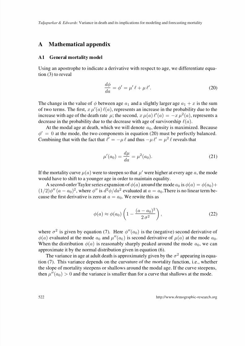
Using an apostrophe to indicate a derivative with respect to age, we differentiate equa-

tion (3) to reveal

dφ

da= φ = µ + µ . (20)

The change in the value of φ between age a1 and a slightly larger age a1 + x is the sum

of two terms. The first, x µ(a) (a), represents an increase in the probability due to the

increase with age of the death rate µ; the second, x µ(a) (a) = −x µ2(a), represents a

decrease in the probability due to the decrease with age of survivorship (a).At the modal age at death, which we will denote a0, density is maximized. Because

φ = 0 at the mode, the two components in equation (20) must be perfectly balanced.

Combining that with the fact that = −µ and thus −µ = µ2 reveals that

µ(a0) =dµ

da= µ2(a0). (21)

If the mortality curve µ(a) were to steepen so that µ were higher at every age a, the mode

would have to shift to a younger age in order to maintain equality.

A second-order Taylor series expansion of φ(a) around the mode a0 is φ(a) = φ(a0)+(1/2)φ (a − a0)2, where φ is d2φ/da2 evaluated at a = a0.There is no linear term be-

cause the first derivative is zero at a = a0. We rewite this as

φ(a) ≈ φ(a0)

1 −

(a − a0)2

2 σ2

, (22)

where σ2 is given by equation (7). Here φ(a0) is the (negative) second derivative of

φ(a) evaluated at the mode a0 and µ(a0) is second derivative of µ(a) at the mode a0.

When the distribution φ(a) is reasonably sharply peaked around the mode a0, we canapproximate it by the normal distribution given in equation (6).

The variance in age at adult death is approximately given by the σ2 appearing in equa-

tion (7). This variance depends on the curvature of the mortality function, i.e., whether

the slope of mortality steepens or shallows around the modal age. If the curve steepens,

then µ(a0) > 0 and the variance is smaller than for a curve that shallows at the mode.


8/7/2019 24-21 demografi



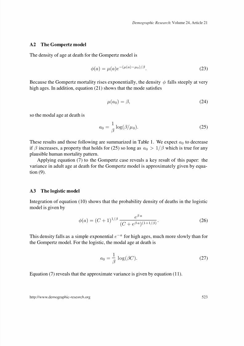
A2 The Gompertz model

The density of age at death for the Gompertz model is

φ(a) = µ(a)e−(µ(a)−µ0)/β. (23)

Because the Gompertz mortality rises exponentially, the density φ falls steeply at very

high ages. In addition, equation (21) shows that the mode satisfies

µ(a0) = β, (24)

so the modal age at death is

a0 =1

β log(β/µ0). (25)

These results and those following are summarized in Table 1. We expect a0 to decrease

if β increases, a property that holds for (25) so long as a0 > 1/β which is true for any

plausible human mortality pattern.

Applying equation (7) to the Gompertz case reveals a key result of this paper: the

variance in adult age at death for the Gompertz model is approximately given by equa-

tion (9).

A3 The logistic model

Integration of equation (10) shows that the probability density of deaths in the logistic

model is given by

φ(a) = (C + 1)1/β eβ a

(C + eβ a)(1+1/β). (26)

This density falls as a simple exponential e−a for high ages, much more slowly than for

the Gompertz model. For the logistic, the modal age at death is

a0 =1

β log(βC ). (27)

Equation (7) reveals that the approximate variance is given by equation (11).


8/7/2019 24-21 demografi



A4 General mortality, multiplicative frailty

Given the mortality function in equation (12), the probability distribution of age at death

isφ(a|Z ) = Z µ(a) exp(−Z M (a)), (28)

with cumulative mortality M (a) defined as in equation (1).

The population probability distribution of age at death is the expectation over frailty,

φ(a) = E [φ(a|Z )] =

g(z) φ(a|z) dz. (29)

Given equation (13), the modal age at death in the population must satisfy

µ(a) = µ2(a)h2

h1

. (30)

Note that if every frailty were equal to 1, we would have h2 = h1 and this equation would

reduce to our earlier equation (21). Also, we have

φ(a0) = h1 µ + µ3

h3 − 3

h22

h1

, (31)

where the hi are evaluated at the mode a0.

A5 General mortality, gamma multiplicative frailty

The gamma distribution in equation (15) is convenient, as Vaupel et al. pointed out,because we can use it with any baseline mortality µ(a) to find an explicit expression for

the population average distribution of age at death, whose general form was given by

equation (29):

φ(a) = µ(a)

k

(k + M (a))

k+1

. (32)

We can differentiate to find that the modal age at death is defined by the condition

µ(a0) =

1 + s2

1 + s2M (a0)

µ2(a0). (33)

Notice that if all individuals had the same frailty, s2 = 0 and equation (33) would reduceto the simpler equation (21). Qualitatively, the denominator on the right describes how

frailty alters the rate of change of average mortality and survival depending on how much

selection acts against more frail individuals. The magnitude of selection depends on both

the variance s2 in frailty, and the cumulative mortality hazard M (a). Strong selection

will act to decrease the modal age at death.


8/7/2019 24-21 demografi



A6 Gompertz mortality, gamma multiplicative frailty

The modal age at death for this model is found using equation (33) with Gompertz mor-

tality as given by equation (8), which yields the condition

µ(a0) = (β − s2µ0). (34)

This reveals an equation for the mode:

a0 =1

β log

β/µ0 − s2

. (35)

Compared with equation (25) for the standard Gompertz, which is shown in the first

column of the third row of Table 1, this equation reveals how frailty acts to reduce the

modal age at death.


8/7/2019 24-21 demografi



24-21 demografi

Documents