22 - storage data structures-v1

Storage Data Structures

1. Notes from review 2. Background

a. File system one type of storage system, with a particular API & semantics i. Point queries, partial object reads/updates, extending objects, large

objects b. Others:

i. Key/value store: point queries ii. DBMS: support point / range queries

c. General question: how do you optimize for different workloads? i. Fast reads: FFS, sequential layout on disk

ii. Fast write: LFS, sequential writes iii. Nova: fast reads/writes via radix-tree indexes

d.

e.

Evolution'of'hard'disks

9

2

0.01

0.1

1

10

100

1000

10000

100000

1000000

10000000

100000000

1950 1960 1970 1980 1990 2000 2010 2020

RPM Latency&(ms)$/GB GB/inFull&Read

0.1&GB/in2

800&GB/in2

SpeedPrice Density

Latency

Full&read

Evolution'of'hard'disks

10

2

0.01

0.1

1

10

100

1000

10000

100000

1000000

10000000

100000000

1950 1960 1970 1980 1990 2000 2010 2020

RPM Latency&(ms)$/GB GB/inFull&Read

8&s

2&h

SpeedPrice Density

Latency

Full&read

f. 3. RUM conjecture:

a. Performance model: i. Assume 2 levels: fast and slow

1. Fast level is free to access (order 1 for most things) but costs space

2. Slow level is expensive to access and costs space ii. Read overhead = # of operations / # of bytes / # of random accesses

beyond amount returned from operation 1. Read 1 block from file: read inode, indirect block, data block: read

overhead of 3 iii. Write overhead = # of operations / # of bytes read or written / # of

random accesses beyond operation 1. FFS extend file: write inode, indirect block, block bitmap, data

block = WO of 4 iv. Memory overhead = how much memory or storage needed

1. Nova extend file: uses log for metadata, so MO = O(N/B) for N bytes, block size B. Uses radix tree = MO = O(log N) for N byte file

2. LFS uses inode map MO = O(M) for M files. b. An access method that can set an upper bound for two out of the read, update,

and memory overheads, also sets a lower bound for the third overhead. c. Hypothesis. An access method that is optimal with respect to one of the read,

update, and memory overheads, cannot achieve the optimal value for both remaining overheads.

Don’t Thrash: How to Cache Your Hash in Flash

Illustration of Optimal Tradeoff [Brodal, Fagerberg 03]

Inserts

Poin

t Q

ueri

es

FastSlow

Slow

Fast

Logging

B-tree

Logging

Optimal Curve

11

d. 4. Examples

a. Read-optimized: QUESTION: what is fastest possible read structure? i. Direct mapped: for a key, look up that location (make an integer)

ii. Read overhead: RO = 1 iii. Write overhead: just write, WO = 1 iv. Space overhead: need space for all possible values, MO = infinity v. How to make it more balanced:

1. Use hashing a. Adds some computation cost on read/write b. Adds O(n) or O(log n) overhead on insert/delete if chaining

used c. Make memory O(N/f) for load factor F

b. Write-optimized design: what is the fastest possible write structure? i. A log: just write at end: WO = 1

ii. Read: scan entire log, read last value, RO = O(N) iii. Memory: O(infinity) as log grows infinite iv. How optimize?

1. Compaction: O(n) inserts occasionally to limit size 2. Add index:binary/B tree O(n) index, O(log n) read or write

c. Memory optimized design i. In a two level system: use O(log n) read/write to go to slower memory, no

index or metadata in memory ii. In a one level system: membership tests with bloom filters

1. Insert: a. Hash value v with K hashes into M bits b. Set K values to 1 in hash

2. Check: a. Hash value V with K hashes b. If all K hashes 1, with high likelihood V was inserted

3. Probability of false negative: zero (bits will be set)

The'RUM'Conjecture

every&access&method&has&a&(quantifiable)• read&overhead• update&overhead• memory&overhead

the&three&of&which&form&a&competing&triangle

Read

Update Memorywe,can,optimize,for,two,of,the,overheads,at,the,expense,of,the,third

22

max

min

minmin

[EDBT2016]

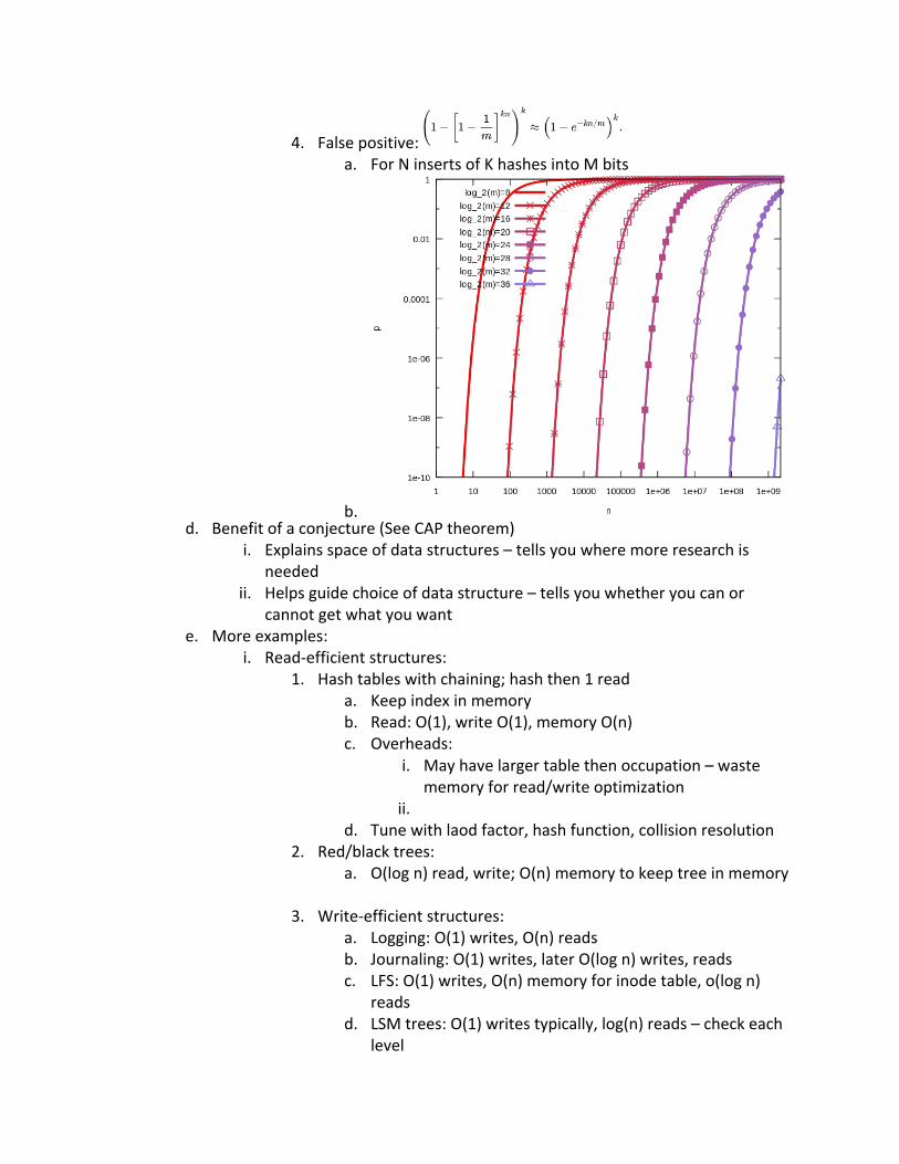
4. False positive: a. For N inserts of K hashes into M bits

b. d. Benefit of a conjecture (See CAP theorem)

i. Explains space of data structures – tells you where more research is needed

ii. Helps guide choice of data structure – tells you whether you can or cannot get what you want

e. More examples: i. Read-efficient structures:

1. Hash tables with chaining; hash then 1 read a. Keep index in memory b. Read: O(1), write O(1), memory O(n) c. Overheads:

i. May have larger table then occupation – waste memory for read/write optimization

ii. d. Tune with laod factor, hash function, collision resolution

2. Red/black trees: a. O(log n) read, write; O(n) memory to keep tree in memory

3. Write-efficient structures:

a. Logging: O(1) writes, O(n) reads b. Journaling: O(1) writes, later O(log n) writes, reads c. LFS: O(1) writes, O(n) memory for inode table, o(log n)

reads d. LSM trees: O(1) writes typically, log(n) reads – check each

level

4. Memory efficient structures a. Dense array: O(n) storage, O(n) read/write b. Bloom filter: O(~n/3) storage

o Examples:

- B-tree (get picture)

-

o o O(log_b N) I/Os – one for each level of tree – log in size of block, overall depends

on data size - Write optimized data structures: incorporate buffering

o Example: balanced binary tree: § O(log N) queries – walk tree from root § O((Log N)/B) inserts for buffer size B – flush at each node when buffer fills

• Flush down a level when fills – cost O(1) for B elements = O(1/B) per item, down O(log N) levels = O((log N)/B) inserts

• NOTE: just for disk cost o Making point queries faster: have fanout sqrt(B)

§ Queries now O(Log sqrt(B) N) not O(log N) § Inserts cost O((Log B N) / sqrt (B)) – more expensive

- Compare logging vs b tree: o Logging has fast inserts, slow point queries (O(1) vs linear) o B-trees have O(Log N) both

- What is the key? o Make inserts fast

§ Allows saving time to build an index o Add indexes to make point queries fast

Don’t Thrash: How to Cache Your Hash in Flash

An algorithmic performance model

B-tree point queries: O(logB N) I/Os.

Binary search in array: O(log N/B)≈O(log N) I/Os.Slower by a factor of O(log B)

O(logBN)

8

B-tree

Lookupmethod&cost?

Anne

Arnold

Yulia

Zack

Corrie

Doug

Bob

Barbara

Anne Bob Corrie … … Yulia

…

…

Anne … …

Depth:O(logB(N/B))

INSTITUTEFORAPPLIEDCOMPUTATIONALSCIENCE

LSM trees (from tutorial – 2013)

- Consider a list of n trees with exponentially increasing size T0 .. Tn, typtically |Tj+1| =

10x |Tj|

- - Point queries: check each of n trees - Range queries: perform range search of each tree, merge results

BasicLSM-tree

Level

0

1

2

3

Buffer

Sortedarrays

X1 ... …

Sort-merge&Eliminateduplicates

… X2 …

… X2 ... … …

Inserts

sort&flushbuffer

Designprinciple#1: optimizeforinsertionsbybuffering

Designprinciple#2: optimizeforlookupsbysort-mergingarrays


Log Structured Merge Tree

An LSM tree is a cascade of B-trees.

Each tree Tj has a target size |Tj | . The target sizes are exponentially increasing.

Typically, target size |Tj+1| = 10 |Tj |.

4

[O'Neil, Cheng, Gawlick, O'Neil 96]

T0 T1 T2 T3 T4

- - Insert: insert into smallest tree

o When fills, flush to next level (re-insert all items)

o - Delete: insert a tombstone in smallest tree

-

LSM Tree Operations

Point queries:

Range queries:

5

T0 T1 T2 T3 T4

T0 T1 T2 T3 T4

LSM Tree Operations

Insertions:• Always insert element into the smallest B-tree T0.

• When a B-tree Tj fills up, flush into Tj+1 .

6

T0 T1 T2 T3 T4

T0 T1 T2 T3 T4

insert

flush

BasicLSM-tree– Lookupcost

Level

0

1

2

3

Buffer

Sortedarrays

… … …

Capacity

1

2

4

8

... ... ... ... ... …

... ... ...

... ... ... ... ... … ... ... ... ... ... …

Lookupmethod? Searchyoungesttooldest. O log& '(

How? Binarysearch. O log& '(

Lookupcost? O log& '(

&


-

- - Analysis:

o Search cost: O(Log N Log B N) – first Log N is for # of trees o Flush cost on overflow a tree: for Tj of size X, cost is O(X/B) – just linear scan

§ Cost per element is O(1B) § # of times each element moved < O(Log N) (# of trees) § Insert cost is O((Log N)/B) – amortized copies

- How accelerate? o Caching

§ Keep small trees in memory - o Bloom filters

§ Bloom filters for out-of-memory trees to avoid useless queries; only search tree where most recent copy is stored

o Fractional cascading § Store forwarding pointers from bottom of Tj tree to interior locations in

TJ+1 - Now: make trees just arrays – not need interior nodes with pointers

BasicLSM-tree– Insertioncost

Level

0

1

2

3

Buffer

Sortedarrays

… … …

Capacity

1

2

4

8

... ... ... ... ... …

... ... ...

... ... ... ... ... … ... ... ... ... ... …

Howmanytimesiseachentrycopied? O log& '(

Whatisthepriceofeachcopy? O )(

Totalinsertcost? O )( * log&

'(


BloomFilters

filters

array… … ... … … … … … X … … …

Answersset-membershipqueriesSmallerthanarray,andstoredinmainmemoryPurpose:avoidaccessingdiskifentryisnotinarraySubtlety:mayreturnfalsepositives.


Bloomfilter

LookupforZ

Accessondisk

https://medium.com/databasss/on-disk-io-part-3-lsm-trees-8b2da218496f LSM trees from Google: using SS tables (sorted string tables)

- SS table: sorted immutable map from key to value, both strings o Immutable so build & write out, never have to insert again

- SS table parts: o Index: keys + offset, can be a data structure (e.g. b-tree) o Data: key + value concatenated

- Updates: against mutable in-memory structure (e.g. B-tree) o When size too big, create new Ss table and write to disk – “flush”

- Read: search in-memory plus all stored SS tables, merge results (remove outdated versions)

- Delete: insert placeholder deleting o Is newest, will be found and overpower older sets o

- Compaction: o Read several SS tables, merge, write out larger Ss table

§ Merge-sort for efficiency §

- Write amplification: o Need to write out multiple times as merge trees o HOWEVER: b-tree must write multiple extra data as well due to block granularity

Other future work:

- Dynamic structures o Build index on the fly o Example: NOVA construct Radix index when open file o Reduces memory at cost of first access

- More dimensions

o

Are'there'more'than'the'R,'U,'M'dimensions?

46

Point&Read Range&Read

Update

DeleteInsert

Memory BgTreeTreeIndex

o

o


47


Update

DeleteInsert

Memory Hash&Index Hash&Index


51


Update

DeleteInsert

MemoryLSMgTree

22 - storage data structures-v1

Documents