2.1  Describing  Location  in  a  Distribution    Here  are  the  scores  of  all  25  students  in  Mr.  Pryor’s  statistics  class  on  their  first  test:    

   The  bold  score  is  Jenny’s  86.  How  did  she  perform  on  this  test  relative  to  her  classmates?    The  stemplot  displays  this  distribution  of  test  scores.  Notice  that  the  distribution  is  roughly  symmetric  with  no  apparent  outliers.  From  the  stemplot,  we  can  see  that  Jenny  did  better  than  all  but  three  students  in  the  class.                              

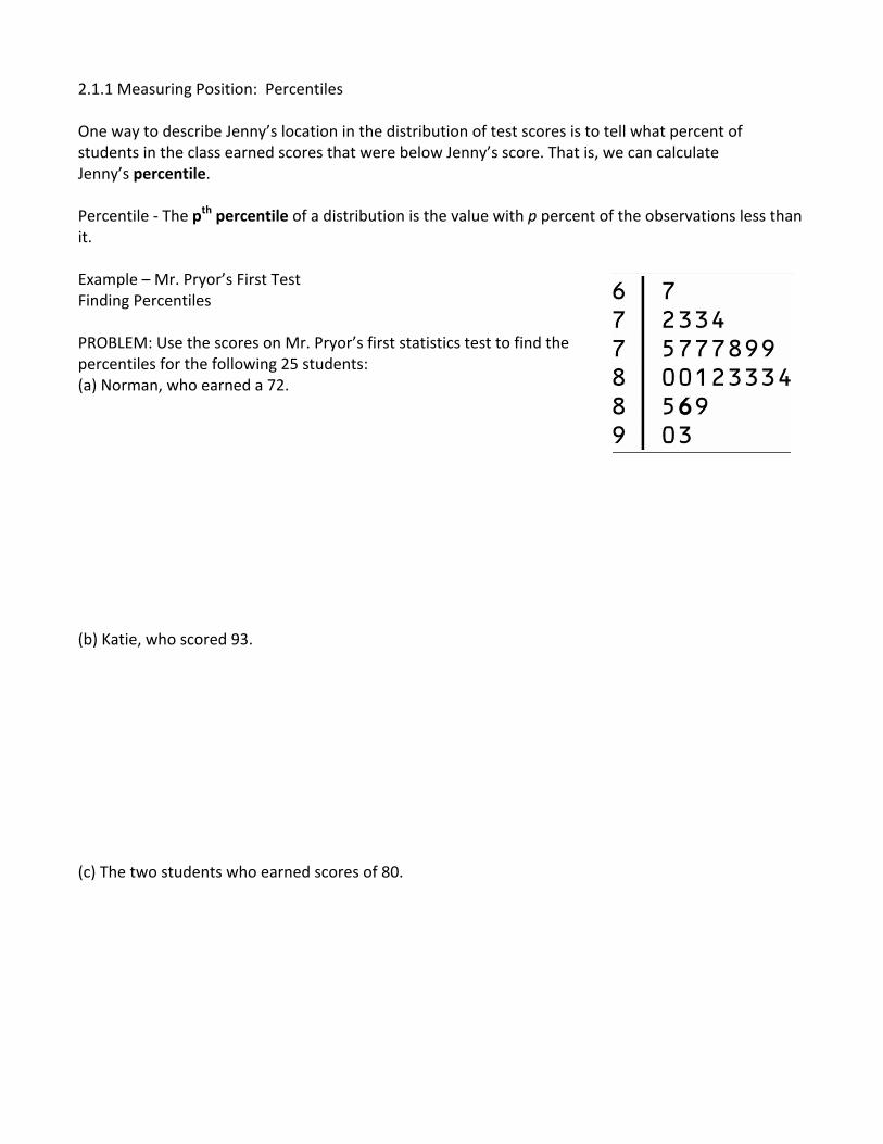
2.1.1  Measuring  Position:    Percentiles    One  way  to  describe  Jenny’s  location  in  the  distribution  of  test  scores  is  to  tell  what  percent  of  students  in  the  class  earned  scores  that  were  below  Jenny’s  score.  That  is,  we  can  calculate  Jenny’s  percentile.    Percentile  -­‐  The  pth  percentile  of  a  distribution  is  the  value  with  p  percent  of  the  observations  less  than  it.    Example  –  Mr.  Pryor’s  First  Test  Finding  Percentiles    PROBLEM:  Use  the  scores  on  Mr.  Pryor’s  first  statistics  test  to  find  the  percentiles  for  the  following  25  students:  (a)  Norman,  who  earned  a  72.                        (b)  Katie,  who  scored  93.                      (c)  The  two  students  who  earned  scores  of  80.          

2.1.2  Cumulative  Relative  Frequency  Graphs    There  are  some  interesting  graphs  that  can  be  made  with  percentiles.  One  of  the  most  common  graphs  starts  with  a  frequency  table  for  a  quantitative  variable.  For  instance,  to  the  right  is  a  frequency  table  that  summarizes  the  ages  of  the  first  44  U.S.  presidents  when  they  were  inaugurated.      Let’s  expand  this  table  to  include  columns  for  relative  frequency,  cumulative  frequency,  and  cumulative  relative  frequency.  

• To  get  the  values  in  the  relative  frequency  column,  divide  the  count  in  each  class  by  44,  the  total  number  of  presidents.  Multiply  by  100  to  convert  to  a  percent.  

• To  fill  in  the  cumulative  frequency  column,  add  the  counts  in  the  frequency  column  for  the  current  class  and  all  classes  with  smaller  values  of  the  variable.  

• For  the  cumulative  relative  frequency  column,  divide  the  entries  in  the  cumulative  frequency  column  by  44,  the  total  number  of  individuals.  Multiply  by  100  to  convert  to  a  percent.  

                   To  make  a  cumulative  relative  frequency  graph,  we  plot  a  point  corresponding  to  the  cumulative  relative  frequency  in  each  class  at  the  smallest  value  of  the  next  class.  For  example,  for  the  40  to  44  class,  we  plot  a  point  at  a  height  of  4.5%  above  the  age  value  of  45.  This  means  that  4.5%  of  presidents  were  inaugurated  before  they  were  45  years  old.  (In  other  words,  age  45  is  the  4.5th  percentile  of  the  inauguration  age  distribution.)  It  is  customary  to  start  a  cumulative  relative  frequency  graph  with  a  point  at  a  height  of  0%  at  the  smallest  value  of  the  first  class  (in  this  case,  40).  The  last  point  we  plot  should  be  at  a  height  of  100%.  We  connect  consecutive  points  with  a  line  segment  to  form  the  graph.  The  figure  below  shows  the  completed  cumulative  relative  frequency  graph.  

   Cumulative  Relative  Frequency  Graph  -­‐  Used  to  examine  location  within  a  distribution.  Cumulative  relative  frequency  graphs  begin  by  grouping  the  observations  into  equal-­‐width  classes.  The  completed  graph  shows  the  accumulating  percent  of  observations  as  you  move  through  the  classes  in  increasing  order.      

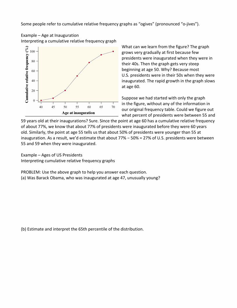
Some  people  refer  to  cumulative  relative  frequency  graphs  as  “ogives”  (pronounced  “o-­‐jives”).    Example  –  Age  at  Inauguration  Interpreting  a  cumulative  relative  frequency  graph  

What  can  we  learn  from  the  figure?  The  graph  grows  very  gradually  at  first  because  few  presidents  were  inaugurated  when  they  were  in  their  40s.  Then  the  graph  gets  very  steep  beginning  at  age  50.  Why?  Because  most  U.S.  presidents  were  in  their  50s  when  they  were  inaugurated.  The  rapid  growth  in  the  graph  slows  at  age  60.    Suppose  we  had  started  with  only  the  graph  in  the  figure,  without  any  of  the  information  in  our  original  frequency  table.  Could  we  figure  out  what  percent  of  presidents  were  between  55  and  

59  years  old  at  their  inaugurations?  Sure.  Since  the  point  at  age  60  has  a  cumulative  relative  frequency  of  about  77%,  we  know  that  about  77%  of  presidents  were  inaugurated  before  they  were  60  years  old.  Similarly,  the  point  at  age  55  tells  us  that  about  50%  of  presidents  were  younger  than  55  at  inauguration.  As  a  result,  we’d  estimate  that  about  77%  −  50%  =  27%  of  U.S.  presidents  were  between  55  and  59  when  they  were  inaugurated.    Example  –  Ages  of  US  Presidents  Interpreting  cumulative  relative  frequency  graphs    PROBLEM:  Use  the  above  graph  to  help  you  answer  each  question.  (a)  Was  Barack  Obama,  who  was  inaugurated  at  age  47,  unusually  young?                  (b)  Estimate  and  interpret  the  65th  percentile  of  the  distribution.    

Percentiles  and  quartiles  Have  you  made  the  connection  between  percentiles  and  the  quartiles  from  Chapter  1?  Earlier,  we  noted  that  the  median  (second  quartile)  corresponds  to  the  50th  percentile.  What  about  the  first  quartile,  Q1?  It’s  at  the  median  of  the  lower  half  of  the  ordered  data,  which  puts  it  about  one-­‐fourth  of  the  way  through  the  distribution.  In  other  words,  Q1  is  roughly  the  25th  percentile.  By  similar  reasoning,  Q3  is  approximately  the  75th  percentile  of  the  distribution.  

CHECK  YOUR  UNDERSTANDING    1. Multiple choice: Select the best answer. Mark receives a score report detailing his performance on a statewide test. On the math section, Mark earned a raw score of 39, which placed him at the 68th percentile. This means that  (a) Mark did better than about 39% of the students who took the test. (b) Mark did worse than about 39% of the students who took the test. (c) Mark did better than about 68% of the students who took the test. (d) Mark did worse than about 68% of the students who took the test. (e) Mark got fewer than half of the questions correct on this test. 2. Mrs. Munson is concerned about how her daughter’s height and weight compare with those of other girls of the same age. She uses an online calculator to determine that her daughter is at the 87th percentile for weight and the 67th percentile for height. Explain to Mrs. Munson what this means.                  Questions 3 and 4 relate to the following setting. The graph displays the cumulative relative frequency of the lengths of phone calls made from the mathematics department office at Gabalot High last month.  

3. About what percent of calls lasted less than 30 minutes? 30 minutes or more?

4. Estimate Q1, Q3, and the IQR of the distribution.

2.1.3  Measuring  Position:  z-­‐Scores    Let’s  return  to  the  data  from  Mr.  Pryor’s  first  statistics  test,  which  are  shown  in  the  stemplot.  The  figure  below  provides  numerical  summaries  from  Minitab  for  these  data.  Where  does  Jenny’s  score  of  86  fall  relative  to  the  mean  of  this  distribution?  Since  the  mean  score  for  the  class  is  80,  we  can  see  that  Jenny’s  score  is  “above  average.”  But  how  much  above  average  is  it?  

               

We  can  describe  Jenny’s  location  in  the  class’s  test  score  distribution  by  telling  how  many  standard  deviations  above  or  below  the  mean  her  score  is.  Since  the  mean  is  80  and  the  standard  deviation  is  about  6,  Jenny’s  score  of  86  is  about  one  standard  deviation  above  the  mean.  Converting  observations  like  this  from  original  values  to  standard  deviation  units  is  known  as  standardizing.  To  standardize  a  value,  subtract  the  mean  of  the  distribution  and  then  divide  by  the  standard  deviation.    Standardized  Value  -­‐  If  X  is  an  observation  from  a  distribution  that  has  known  mean  and  standard  deviation,  the  standardized  value  of  X  is:          A  standardized  value  is  often  called  a  z-­‐score.    A  z-­‐score  tells  us  how  many  standard  deviations  from  the  mean  an  observation  falls,  and  in  what  direction.  Observations  larger  than  the  mean  have  positive  z-­‐scores;  observations  smaller  than  the  mean  have  negative  z-­‐scores.  For  example,  Jenny’s  score  on  the  test  was  x  =  86.  Her  standardized  score  (z-­‐score)  is:            That  is,  Jenny’s  test  score  is  about  one  standard  deviation  above  the  mean  score  of  the  class.    

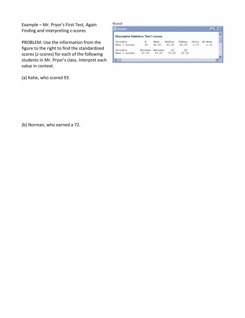
Example  –  Mr.  Pryor’s  First  Test,  Again  Finding  and  interpreting  z-­‐scores    PROBLEM:  Use  the  information  from  the  figure  to  the  right  to  find  the  standardized  scores  (z-­‐scores)  for  each  of  the  following  students  in  Mr.  Pryor’s  class.  Interpret  each  value  in  context.    (a)  Katie,  who  scored  93.                (b)  Norman,  who  earned  a  72.                

We  can  also  use  z-­‐scores  to  compare  the  position  of  individuals  in  different  distributions,  as  the  following  example  illustrates.    Example  -­‐  Jenny  Takes  Another  Test  Using  z-­‐scores  for  comparisons    The  day  after  receiving  her  statistics  test  result  of  86  from  Mr.  Pryor,  Jenny  earned  an  82  on  Mr.  Goldstone’s  chemistry  test.  At  first,  she  was  disappointed.  Then  Mr.  Goldstone  told  the  class  that  the  distribution  of  scores  was  fairly  symmetric  with  a  mean  of  76  and  a  standard  deviation  of  4.    Problem:    On  which  test  did  Jenny  perform  better  relative  to  the  class?  Justify  your  answer.                  We  often  standardize  observations  to  express  them  on  a  common  scale.  We  might,  for  example,  compare  the  heights  of  two  children  of  different  ages  by  calculating  their  z-­‐scores.  At  age  2,  Jordan  is  89  centimeters  (cm)  tall.  Her  height  puts  her  at  a  z-­‐score  of  0.5;  that  is,  she  is  one-­‐half  standard  deviation  above  the  mean  height  of  2-­‐year-­‐old  girls.  Zayne’s  height  at  age  3  is  101  cm,  which  yields  a  z-­‐score  of  1.  In  other  words,  he  is  one  standard  deviation  above  the  mean  height  of  3-­‐year-­‐old  boys.  So  Zayne  is  taller  relative  to  boys  his  age  than  Jordan  is  relative  to  girls  her  age.  The  standardized  heights  tell  us  where  each  child  stands  (pun  intended!)  in  the  distribution  for  his  or  her  age  group.    

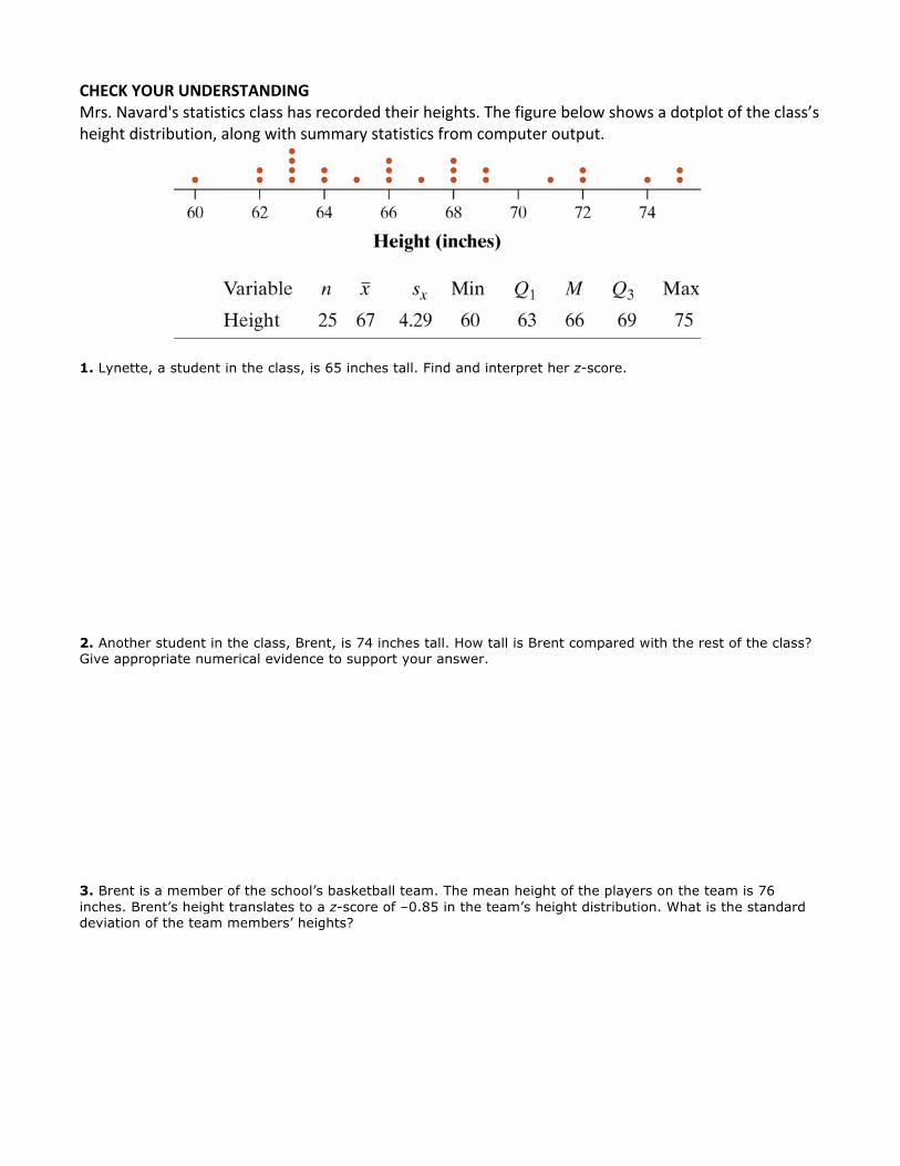
CHECK  YOUR  UNDERSTANDING  Mrs.  Navard's  statistics  class  has  recorded  their  heights.  The  figure  below  shows  a  dotplot  of  the  class’s  height  distribution,  along  with  summary  statistics  from  computer  output.                      1. Lynette, a student in the class, is 65 inches tall. Find and interpret her z-score.                   2. Another student in the class, Brent, is 74 inches tall. How tall is Brent compared with the rest of the class? Give appropriate numerical evidence to support your answer.                    3. Brent is a member of the school’s basketball team. The mean height of the players on the team is 76 inches. Brent’s height translates to a z-score of –0.85 in the team’s height distribution. What is the standard deviation of the team members’ heights?      

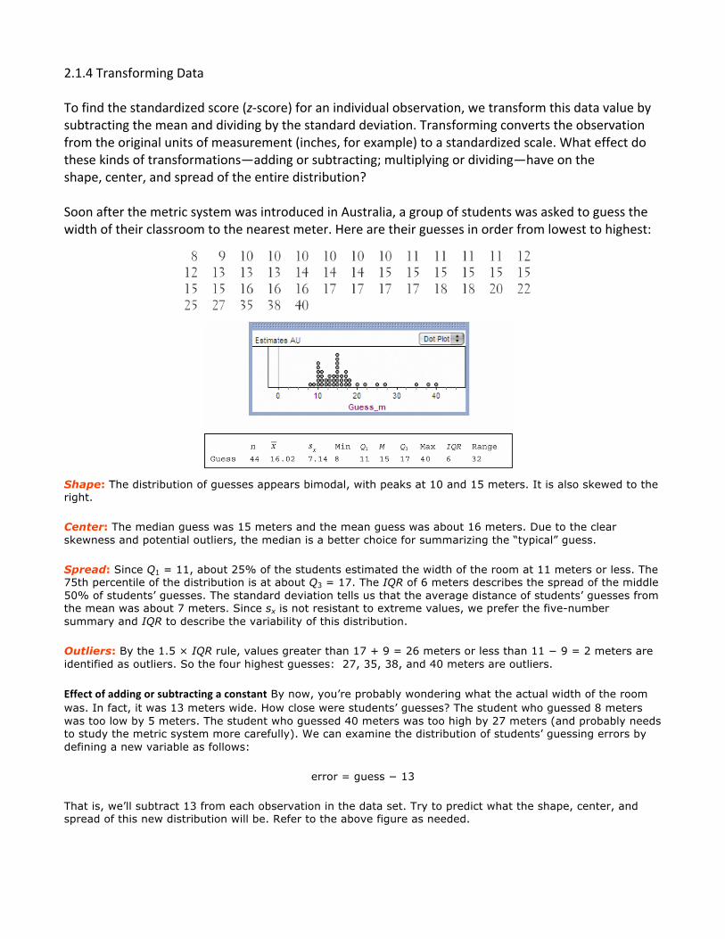
2.1.4  Transforming  Data    To  find  the  standardized  score  (z-­‐score)  for  an  individual  observation,  we  transform  this  data  value  by  subtracting  the  mean  and  dividing  by  the  standard  deviation.  Transforming  converts  the  observation  from  the  original  units  of  measurement  (inches,  for  example)  to  a  standardized  scale.  What  effect  do  these  kinds  of  transformations—adding  or  subtracting;  multiplying  or  dividing—have  on  the  shape,  center,  and  spread  of  the  entire  distribution?    Soon  after  the  metric  system  was  introduced  in  Australia,  a  group  of  students  was  asked  to  guess  the  width  of  their  classroom  to  the  nearest  meter.  Here  are  their  guesses  in  order  from  lowest  to  highest:    

                       

Shape: The distribution of guesses appears bimodal, with peaks at 10 and 15 meters. It is also skewed to the right.

Center: The median guess was 15 meters and the mean guess was about 16 meters. Due to the clear skewness and potential outliers, the median is a better choice for summarizing the “typical” guess.

Spread: Since Q1 = 11, about 25% of the students estimated the width of the room at 11 meters or less. The 75th percentile of the distribution is at about Q3 = 17. The IQR of 6 meters describes the spread of the middle 50% of students’ guesses. The standard deviation tells us that the average distance of students’ guesses from the mean was about 7 meters. Since sx is not resistant to extreme values, we prefer the five-number summary and IQR to describe the variability of this distribution.

Outliers: By the 1.5 × IQR rule, values greater than 17 + 9 = 26 meters or less than 11 − 9 = 2 meters are identified as outliers. So the four highest guesses: 27, 35, 38, and 40 meters are outliers.

Effect  of  adding  or  subtracting  a  constant By now, you’re probably wondering what the actual width of the room was. In fact, it was 13 meters wide. How close were students’ guesses? The student who guessed 8 meters was too low by 5 meters. The student who guessed 40 meters was too high by 27 meters (and probably needs to study the metric system more carefully). We can examine the distribution of students’ guessing errors by defining a new variable as follows:

error = guess − 13

That is, we’ll subtract 13 from each observation in the data set. Try to predict what the shape, center, and spread of this new distribution will be. Refer to the above figure as needed.

Example  Effect  of  subtracting  a  constant    Let’s  see  how  accurate  your  predictions  were  (you  did  make  predictions,  right?).    The  figure  below  shows  dotplots  of  students’  original  guesses  and  their  errors  on  the  same  scale.  We  can  see  that  the  original  distribution  of  guesses  has  been  shifted  to  the  left.  By  how  much?  Since  the  peak  at  15  meters  in  the  original  graph  is  located  at  2  meters  in  the  error  distribution,  the  original  data  values  have  been  translated  13  units  to  the  left.  That  should  make  sense:  we  calculated  the  errors  by  subtracting  the  actual  room  width,  13  meters,  from  each  student’s  guess.                        From  the  figure  above,  it  seems  clear  that  subtracting  13  from  each  observation  did  not  affect  the  shape  or  spread  of  the  distribution.  But  this  transformation  appears  to  have  decreased  the  center  of  the  distribution  by  13  meters.  The  summary  statistics  in  the  table  below  confirm  our  beliefs.            The  error  distribution  is  centered  at  a  value  that  is  clearly  positive—the  median  error  is  2  meters  and  the  mean  error  is  3  meters.  So  the  students  generally  tended  to  overestimate  the  width  of  the  room.    

   

Effect  of  multiplying  or  dividing  by  a  constant  Since  our  group  of  Australian  students  is  having  some  difficulty  with  the  metric  system,  it  may  not  be  very  helpful  to  tell  them  that  their  guesses  tended  to  be  about  2  to  3  meters  too  high.  Let’s  convert  the  error  data  to  feet  before  we  report  back  to  them.  There  are  roughly  3.28  feet  in  a  meter.  So  for  the  student  whose  error  was  −5  meters,  that  translates  to          To  change  the  units  of  measurement  from  meters  to  feet,  we  need  to  multiply  each  of  the  error  values  by  3.28.  What  effect  will  this  have  on  the  shape,  center,  and  spread  of  the  distribution?    Example  -­‐  Estimating  Room  Width  Effect  of  multiplying  by  a  constant    The  figure  below  includes  dotplots  of  the  students’  guessing  errors  in  meters  and  feet,  along  with  summary  statistics  from  computer  software.  The  shape  of  the  two  distributions  is  the  same—bimodal  and  right-­‐skewed.  However,  the  centers  and  spreads  of  the  two  distributions  are  quite  different.  The  bottom  dotplot  is  centered  at  a  value  that  is  to  the  right  of  the  top  dotplot’s  center.  In  addition,  the  bottom  dotplot  shows  much  greater  spread  than  the  top  dotplot.    When  the  errors  were  measured  in  meters,  the  median  was  2  and  the  mean  was  3.02.For  the  transformed  error  data  in  feet,  the  median  is  6.56  and  the  mean  is  9.91.  Can  you  see  that  the  measures  of  center  were  multiplied  by  3.28?  That  makes  sense—if  we  multiply  all  of  the  observations  by  3.28,  then  the  mean  and  median  should  also  be  multiplied  by  3.28.    What  about  the  spread?  Multiplying  each  observation  by  3.28  increases  the  variability  of  the  distribution.  By  how  much?  You  guessed  it—by  a  factor  of  3.28.  The  numerical  summaries  in  the  figure  below  show  that  the  standard  deviation  sx,  the  interquartile  range,  and  the  range  have  been  multiplied  by  3.28.    We  can  safely  tell  our  group  of  Australian  students  that  their  estimates  of  the  classroom’s  width  tended  to  be  too  high  by  about  6.5  feet.  (Notice  that  we  choose  not  to  report  the  mean  error,  which  is  affected  by  the  strong  skewness  and  the  three  high  outliers.)                            

 

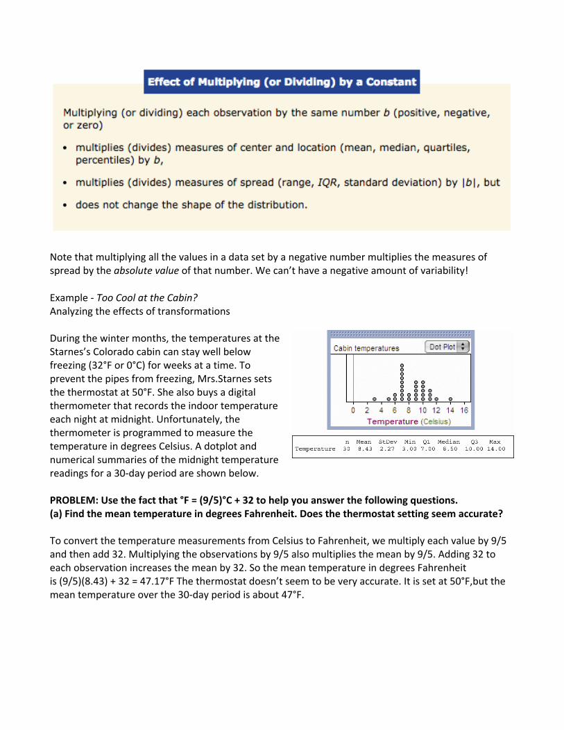
   Note  that  multiplying  all  the  values  in  a  data  set  by  a  negative  number  multiplies  the  measures  of  spread  by  the  absolute  value  of  that  number.  We  can’t  have  a  negative  amount  of  variability!    Example  -­‐  Too  Cool  at  the  Cabin?  Analyzing  the  effects  of  transformations    During  the  winter  months,  the  temperatures  at  the  Starnes’s  Colorado  cabin  can  stay  well  below  freezing  (32°F  or  0°C)  for  weeks  at  a  time.  To  prevent  the  pipes  from  freezing,  Mrs.Starnes  sets  the  thermostat  at  50°F.  She  also  buys  a  digital  thermometer  that  records  the  indoor  temperature  each  night  at  midnight.  Unfortunately,  the  thermometer  is  programmed  to  measure  the  temperature  in  degrees  Celsius.  A  dotplot  and  numerical  summaries  of  the  midnight  temperature  readings  for  a  30-­‐day  period  are  shown  below.    PROBLEM:  Use  the  fact  that  °F  =  (9/5)°C  +  32  to  help  you  answer  the  following  questions.  (a)  Find  the  mean  temperature  in  degrees  Fahrenheit.  Does  the  thermostat  setting  seem  accurate?    To  convert  the  temperature  measurements  from  Celsius  to  Fahrenheit,  we  multiply  each  value  by  9/5  and  then  add  32.  Multiplying  the  observations  by  9/5  also  multiplies  the  mean  by  9/5.  Adding  32  to  each  observation  increases  the  mean  by  32.  So  the  mean  temperature  in  degrees  Fahrenheit  is  (9/5)(8.43)  +  32  =  47.17°F  The  thermostat  doesn’t  seem  to  be  very  accurate.  It  is  set  at  50°F,but  the  mean  temperature  over  the  30-­‐day  period  is  about  47°F.          

(b)  Calculate  the  standard  deviation  of  the  temperature  readings  in  degrees  Fahrenheit.  Interpret  this  value  in  context.    Multiplying  each  observation  by  9/5  multiplies  the  standard  deviation  by  9/5.  However,  adding  32  to  each  observation  doesn’t  affect  the  spread.  So  the  standard  deviation  of  the  temperature  measurements  in  degrees  Fahrenheit  is(9/5)(2.27)  =  4.09°F.  This  means  that  the  average  distance  of  the  temperature  readings  from  the  mean  is  about  4°F.  That’s  a  lot  of  variation!    (c)  The  90th  percentile  of  the  temperature  readings  was  11°C.  What  is  the  90th  percentile  temperature  in  degrees  Fahrenheit?    Both  multiplying  by  a  constant  and  adding  a  constant  affect  the  value  of  the  90th  percentile.  To  find  the  90th  percentile  in  degrees  Fahrenheit,  we  need  to  multiply  the  90th  percentile  in  degrees  Celsius  by  9/5  and  then  add  32:  (9/5)(11)  +  32  =  51.8°F.      Connecting  transformations  and  z-­‐scores  What  does  all  this  transformation  business  have  to  do  with  z-­‐scores?  To  standardize  an  observation,  you  subtract  the  mean  of  the  distribution  and  then  divide  by  the  standard  deviation.  What  if  we  standardized  every  observation  in  a  distribution?    If we standardize every observation in a distribution, the resulting set of z-scores has mean 0 and standard deviation 1

CHECK  YOUR  UNDERSTANDING    The figure to the right shows a dotplot of the height distribution for Mrs. Navard’s class, along with summary statistics from computer output. 1. Suppose that you convert the class’s heights from inches to centimeters (1 inch = 2.54 cm). Describe the effect this will have on the shape, center, and spread of the distribution. 2. If Mrs. Navard had the entire class stand on a 6-inch-high platform and then had the students measure the distance from the top of their heads to the ground, how would the shape, center, and spread of this distribution compare with the original height distribution? 3. Now suppose that you convert the class’s heights to z-scores. What would be the shape, center, and spread of this distribution? Explain.

2.1.5  Density  Curves    You  learned  from  chapter  1…  

   Now  we  add...    

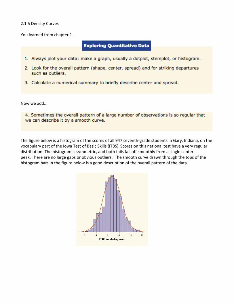
   The  figure  below  is  a  histogram  of  the  scores  of  all  947  seventh-­‐grade  students  in  Gary,  Indiana,  on  the  vocabulary  part  of  the  Iowa  Test  of  Basic  Skills  (ITBS).  Scores  on  this  national  test  have  a  very  regular  distribution.  The  histogram  is  symmetric,  and  both  tails  fall  off  smoothly  from  a  single  center  peak.  There  are  no  large  gaps  or  obvious  outliers.    The  smooth  curve  drawn  through  the  tops  of  the  histogram  bars  in  the  figure  below  is  a  good  description  of  the  overall  pattern  of  the  data.                              

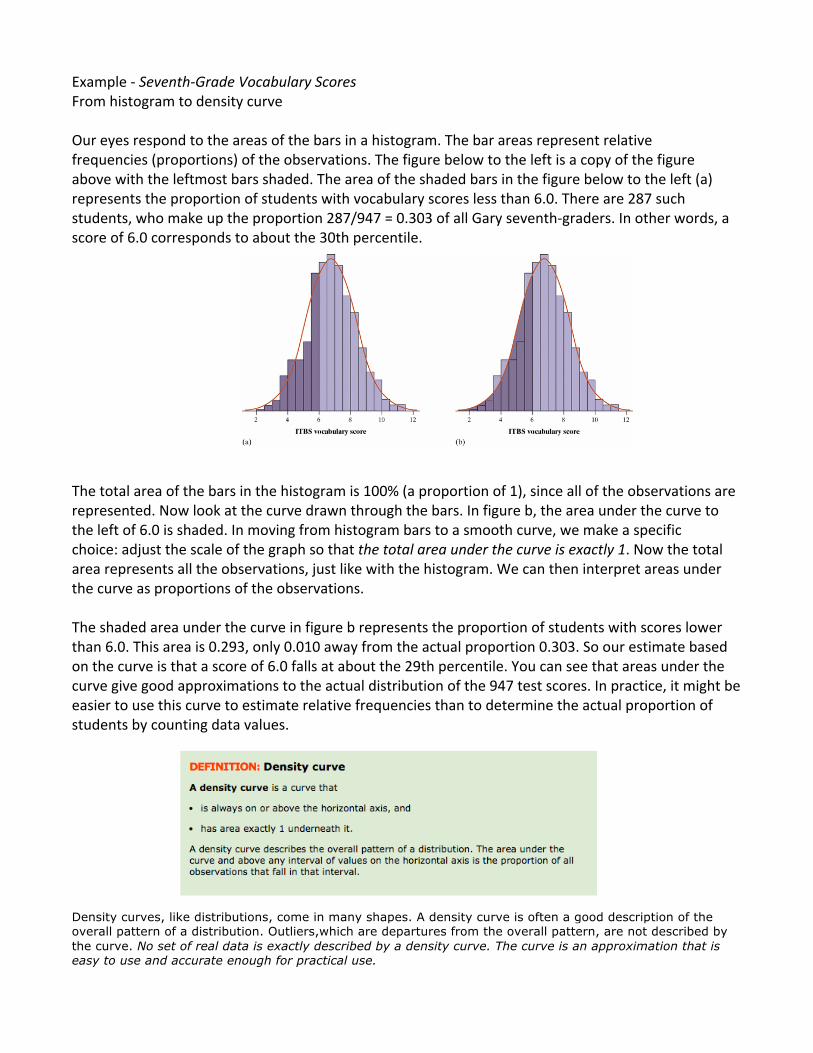
Example  -­‐  Seventh-­‐Grade  Vocabulary  Scores  From  histogram  to  density  curve    Our  eyes  respond  to  the  areas  of  the  bars  in  a  histogram.  The  bar  areas  represent  relative  frequencies  (proportions)  of  the  observations.  The  figure  below  to  the  left  is  a  copy  of  the  figure  above  with  the  leftmost  bars  shaded.  The  area  of  the  shaded  bars  in  the  figure  below  to  the  left  (a)  represents  the  proportion  of  students  with  vocabulary  scores  less  than  6.0.  There  are  287  such  students,  who  make  up  the  proportion  287/947  =  0.303  of  all  Gary  seventh-­‐graders.  In  other  words,  a  score  of  6.0  corresponds  to  about  the  30th  percentile.                          The  total  area  of  the  bars  in  the  histogram  is  100%  (a  proportion  of  1),  since  all  of  the  observations  are  represented.  Now  look  at  the  curve  drawn  through  the  bars.  In  figure  b,  the  area  under  the  curve  to  the  left  of  6.0  is  shaded.  In  moving  from  histogram  bars  to  a  smooth  curve,  we  make  a  specific  choice:  adjust  the  scale  of  the  graph  so  that  the  total  area  under  the  curve  is  exactly  1.  Now  the  total  area  represents  all  the  observations,  just  like  with  the  histogram.  We  can  then  interpret  areas  under  the  curve  as  proportions  of  the  observations.    The  shaded  area  under  the  curve  in  figure  b  represents  the  proportion  of  students  with  scores  lower  than  6.0.  This  area  is  0.293,  only  0.010  away  from  the  actual  proportion  0.303.  So  our  estimate  based  on  the  curve  is  that  a  score  of  6.0  falls  at  about  the  29th  percentile.  You  can  see  that  areas  under  the  curve  give  good  approximations  to  the  actual  distribution  of  the  947  test  scores.  In  practice,  it  might  be  easier  to  use  this  curve  to  estimate  relative  frequencies  than  to  determine  the  actual  proportion  of  students  by  counting  data  values.                    Density curves, like distributions, come in many shapes. A density curve is often a good description of the overall pattern of a distribution. Outliers,which are departures from the overall pattern, are not described by the curve. No set of real data is exactly described by a density curve. The curve is an approximation that is easy to use and accurate enough for practical use.

2.1.6  Describing  Density  Curves  Our  measures  of  center  and  spread  apply  to  density  curves  as  well  as  to  actual  sets  of  observations.  Areas  under  a  density  curve  represent  proportions  of  the  total  number  of  observations.  The  median  of  a  data  set  is  the  point  with  half  the  observations  on  either  side.  So  the  median  of  a  density  curve  is  the  “equal-­‐areas  point,”  the  point  with  half  the  area  under  the  curve  to  its  left  and  the  remaining  half  of  the  area  to  its  right.    

   Because  a  density  curve  is  an  idealized  description  of  a  distribution  of  data,  we  need  to  distinguish  between  the  mean  and  standard  deviation  of  the  density  curve  and  the  mean    and  standard  deviation  sx  computed  from  the  actual  observations.  The  usual  notation  for  the  mean  of  a  density  curve  is  μ  (the  Greek  letter  mu).  We  write  the  standard  deviation  of  a  density  curve  as  σ  (the  Greek  letter  sigma).  We  can  roughly  locate  the  mean  μ  of  any  density  curve  by  eye,  as  the  balance  point.  There  is  no  easy  way  to  locate  the  standard  deviation  σ  by  eye  for  density  curves  in  general.                                        

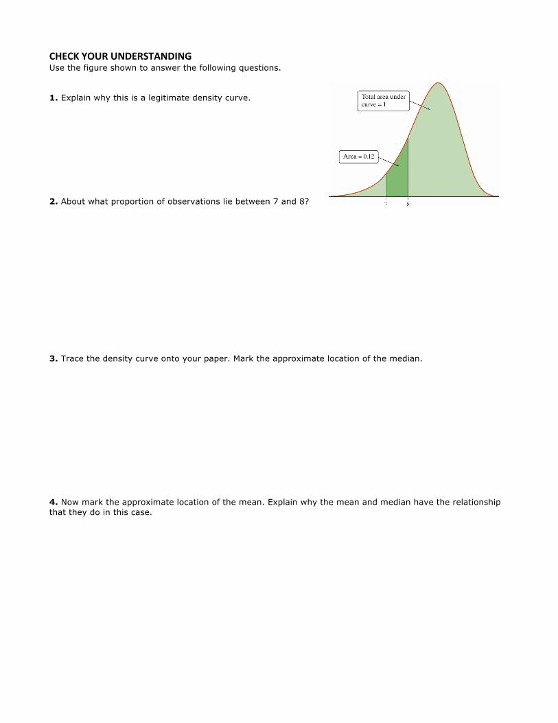
CHECK  YOUR  UNDERSTANDING  Use the figure shown to answer the following questions. 1. Explain why this is a legitimate density curve.              2. About what proportion of observations lie between 7 and 8?                      3. Trace the density curve onto your paper. Mark the approximate location of the median.                    4. Now mark the approximate location of the mean. Explain why the mean and median have the relationship that they do in this case.