vrahli.github.io · 2020-03-06 · fundamenta informaticae xxi (2001) 1001–1032 1001 ios press on...
TRANSCRIPT

Fundamenta Informaticae XXI (2001) 1001–1032 1001
IOS Press
On Realisability Semantics for Intersection Types with ExpansionVariables
Fairouz Kamareddine
ULTRA Group (Useful Logics, Types, Rewriting, and their Automation), Heriot-Watt University,
School of Mathematical and Computer Sciences, Edinburgh EH14 4AS, UK.
Email: http://www.macs.hw.ac.uk/ultra/
Karim Nour
Universite de Savoie, Campus Scientifique, 73378 Le Bourget du Lac, France.
Email: [email protected]
Vincent Rahli∗
and J. B. Wells†
Abstract. Expansion is a crucial operation for calculating principaltypings in intersection type sys-tems. Because the early definitions of expansion were complicated,E-variableswere introducedin order to make the calculations easier to mechanise and reason about. Recently, E-variables havebeen further simplified and generalised to also allow calculating other type operators than just in-tersection. There has been much work on semantics for type systems with intersection types, butnone whatsoever before our work, on type systems with E-variables. In this paper we expose thechallenges of building a semantics for E-variables and we provide a novel solution. Because it isunclear how to devise a space of meanings for E-variables, wedevelop instead a space of meaningsfor types that is hierarchical. First, we index each type with a natural number and show that althoughthis intuitively captures the use of E-variables, it is difficult to index the universal typeω with thishierarchy and it is not possible to obtain completeness of the semantics if more than one E-variableis used. We then move to a more complex semantics where each type is associated with a list ofnatural numbers and establish that bothω and an arbitrary number of E-variables can be representedwithout losing any of the desirable properties of a realisability semantics.
Keywords: Realisability semantics, expansion variables, intersection types, completeness
Address for correspondence: ULTRA Group (Useful Logics, Types, Rewriting, and their Automation), Heriot-WattUniversity, School of Mathematical and Computer Sciences,Mountbatten building, Edinburgh EH14 4AS, UK. Email:http://www.macs.hw.ac.uk/ultra/∗Same address as Kamareddine.†Same address as Kamareddine.
1002 Kamareddine, Nour, Rahli, Wells / semantics of expansion variables
1. Introduction
Intersection types and the expansion mechanism. Intersection types were developed in the late1970s to typeλ-terms that are untypable with simple types; they do this by providing a kind of finitarytype polymorphism where the usages (types) of terms are listed rather than obtained by quantification.They have been useful in reasoning about the semantics of theλ-calculus, and have been investigated foruse in static program analysis.Expansionwas introduced at the end of the 1970s as a crucial procedurefor calculatingprincipal typingsfor λ-terms in type systems with intersection types, allowing supportfor compositional type inference. Coppo, Dezani, and Venneri [7] introduced the operation ofexpansionon typings(pairs of a type environment and a result type) for calculating the possible typings of a termwhen using intersection types. As a simple example, there exists an intersection type systemS wheretheλ-termM = (λx.x(λy.yz)) can be assigned the typingΦ1 = 〈{z 7→ a}, (((a�b)�b)�c)�c〉, whichhappens to be its principal typing inS. The termM can also be assigned the typingΦ2 = 〈s{z 7→ a1 ⊓a2}, ((((a1�b1)�b1) ⊓ ((a2�b2)�b2))�c)�c〉, and an expansion operation can yieldΦ2 from Φ1.
Expansion variables. Because the early definitions of expansion were complicated, E-variableswereintroduced in order to make the calculations easier to mechanize and reason about. For example, inSystem E [5], the typingΦ1 presented above is replaced byΦ3 = 〈{z 7→ ea}, ((e((a�b)�b))�c)�c〉,which differs fromΦ1 by the insertion of the E-variablee at two places (in both components of theΦ3),andΦ2 can be obtained fromΦ3 by substituting fore theexpansion termE = (a := a1, b := b1)⊓ (a :=a2, b := b2). Carlier and Wells [6] have surveyed the history of expansion and also E-variables.
Designing a space of meanings for expansion variables. In many kinds of semantics, a typeTis interpreted by a second order function[T ]ν that takes two parameters, the typeT and also a valuationν that assigns to type variables the same kind of meanings thatare assigned to types. To extend this ideato types with E-variables, we need to devise some space of possible meanings for E-variables. Given thata typeeT can be turned by expansion into a new typeS1(T )⊓S2(T ), whereS1 andS2 are arbitrary sub-stitutions (which can themselves introduce expansions), and that this can introduce an unbound numberof new variables (both E-variables and regular type variables), the situation is complicated. Because it isunclear how to devise a space of meanings for expansions and E-variables, we instead restrict ourselvesto E-variables and develop a space of meanings for types thatis hierarchical in the sense that we can splitit w.r.t. a certain concept of degree. Although this idea is not perfect, it seems to go quite far in giving anintuition for E-variables, namely that each E-variable occurring in a typing associated with aλ-term, actsas a capsule that isolates parts of theλ-term. As future work, we wish to come up with a higher orderfunction that interprets types involving expansion terms by sets ofλ-terms. We believe this functionwould help regarding the substitution mechanism introduced by expansion in terms ofλ-expressions.
Our semantic approach. The semantic approach we use in the current document is a realisabilitysemantics in the sense that it is derived from Kreisel’s modified realisability and its variants, where “aformula “x realizesA” can be defined in a completely straightforward way: the typeof the variablexis determined by the logical form ofA” [26], x being the code of a function. Our semantics is stronglyrelated to the semantic argument used in reducibility methods as used and developed by Tait [27] andmany others after him [24, 23, 13, 12, 14, 15]. Atomic types (e.g., type variables) are interpreted assaturatedsets ofλ-terms, meaning that they are closed underβ-expansion (the inverse ofβ-reduction).Arrow types are interpreted by function spaces (see the semantics provided by Scott in the open problems

Kamareddine, Nour, Rahli, Wells / semantics of expansion variables 1003
published in the proceedings of the Lecture Notes in Computer Science symposium held in 1975 [4]) andintersection types are interpreted by set intersections. Such a realisability semantics allows one to provesoundnessw.r.t. a type systemS, i.e., the meaning of a typeT contains all closedλ-terms that can beassignedT in S. This has been shown useful for characterising the behaviour of typedλ-terms [24]. Onealso wants to show the converse of soundness which is calledcompleteness, i.e., every closedλ-term inthe meaning ofT can be assignedT in S.
Completeness results. Hindley [17, 18, 19] was one of the first to investigate such completenessresults for a simple type system and he showed that all the types of that system have the completenessproperty. He then generalised his completeness proof to an intersection type system [16]. Using his com-pleteness theorem based on saturated sets ofλ-terms w.r.t.βη-equivalence, Hindley showed that simpletypes were “realised”1 by all and only theλ-terms which are typable by these types. Note that Hindley’scompleteness theorems were established with the sets ofλ-terms saturated byβη-equivalence. In thepresent document, our completeness result depends only on the weaker requirement ofβ-equivalence,and we have managed to make simpler proofs that avoid needingη-reduction, confluence, or SN (al-though we do establish both confluence and SN for bothβ andβη).
Similar approaches to type interpretation. Recent works on realisability related to ours includethat by Labib-Sami [25], Farkh and Nour [11], and Coquand [9], although none of this work deals withintersection types or E-variables. Similar work on realisability dealing with intersection types includesthat by Kamareddine and Nour [21], which gives a sound and complete realisability semantics w.r.t. anintersection type system. This system does not deal with E-variables and is therefore different from thethree hierarchical systems presented in this document. Themain difference is the hierarchies which didnot exist in Kamareddine and Nour’s document [21].
Towards a semantics of expansion. Initially, we aimed to give a realisability semantics for asystem of expansions proposed by Carlier and Wells [6]. In order to simplify our study, we consideredthe system with expansion variables but without the expansion rewriting rules (without the expansionmechanism). In essence, this meant that the type syntax was:T ∈ Ty ::= a | ω | T1�T2 | T1 ⊓ T2 | eTwherea is a type variable ranging over a countably infinite type variable setTyVar ande is an expansionvariable ranging over a countably infinite expansion variable setExpVar, and that the typing rules wereas follows:
x : 〈{x 7→T } ⊢ T 〉(var)
M : 〈∅ ⊢ ω〉(ω)
M : 〈Γ ⊎ {x 7→T1} ⊢ T2〉
λx.M : 〈Γ ⊢ T1�T2〉(abs)
M1 : 〈Γ1 ⊢ T1�T2〉 M2 : 〈Γ2 ⊢ T1〉
M1M2 : 〈Γ1 ⊓ Γ2 ⊢ T2〉(app)
M : 〈Γ1 ⊢ T1〉 M : 〈Γ2 ⊢ T2〉
M : 〈Γ1 ⊓ Γ2 ⊢ T1 ⊓ T2〉(⊓)
M : 〈Γ ⊢ T 〉
M : 〈eΓ ⊢ eT 〉(e-app)
To provide a realisability semantics for this system, we needed to define the interpretation of a typeto be a set of terms having this type. For our semantics to be informative on expansion variables, weneeded to distinguish between the interpretation ofT and eT . However, in the typing rule(e-app)
1We say that aλ-termM “realises” a typeT if M is in T ’s interpretation. Hindley’s semantics is not a realisability semanticsbut it bears some resemblance with modified realisability. One of Hindley’s semantics is called “the simple semantics” and isbased on the concept of model of the untypedλ-calculus [20]. Our type interpretation is also similar to Hindley’s[16].
1004 Kamareddine, Nour, Rahli, Wells / semantics of expansion variables
presented above, the termM is unchanged and this poses difficulties. For this reason, wemodifiedslightly the above type system by indexing the terms of theλ-calculus giving us the following syntax ofterms:M ::= xi | (MN) | (λxi.M) (whereM andN need to satisfy a certain condition before(MN)is allowed to be a term) and by slightly changing our type rules and in particular rule(e-app):
M : 〈Γ ⊢ U〉
M+ : 〈eΓ ⊢ eU〉(e-app)
In this new(e-app) rule, M+ is M where all the indices are increased by 1. Obviously these indicesneeded a revision regardingβ-reduction and the typing rules in order to preserve the desirable propertiesof the type system and the realisability semantics. For this, we defined the good terms and the good typesand showed that these notions go hand in hand (e.g., good types can only be assigned to good terms).
We developed a realisability semantics where each use of an E-variable in a type corresponds to anindex at which evaluation occurs in theλ-terms that are assigned the type. This was an elegant solutionthat captured the intuition behind E-variables. However, in order for this new type system to behavewell, it was necessary to considerλI-terms only (removing a subterm fromM also removes importantinformation aboutM as in the reduction(λx.y)M →β y whereM is thrown away). It was also necessaryto drop the universal typeω completely. This led us to the introduction of theλIN-calculus and to ourfirst type system⊢1 for which we developed a sound realisability semantics for E-variables.
However, although the first type system⊢1 is crucial to understand the intuition behind out indexedcalculus, the realisability semantics we proposed was not complete w.r.t.⊢1 (subject reduction does nothold either). For this reason, we modified our system⊢1 by considering a smaller set of types (whereintersections and expansions cannot occur directly to the right of an arrow), and by adding subtypingrules. This new type system⊢2 has subject reduction. Our semantics turned out to be sound w.r.t. ⊢2.As for completeness, we needed to limit the list of expansionvariables to a single element list. Thiscompleteness issue for⊢2 comes from the fact that the natural numbers as indexes do notallow one todifferentiate between the typese1T ande2T if e1 6= e2. Again, we were forced to revise our type system.We decided to restrict ourλ-terms by indexing them by lists of natural numbers (where each naturalnumber represents a difference expansion variable). We updated the type system⊢2 in consequence toobtain the type system⊢3 based among other things on the following new(e-app) rule:
M : 〈Γ ⊢ U〉
M+i : 〈eΓ ⊢ eU〉(e-app)
wherei is the natural number associated with the expansion variable e and whereM+i is M where allthe lists of natural numbers are augmented withi. This new rule(e-app) allows us to distinguish theinterpretations of the typese1T ande2T whene1 6= e2. Furthermore, ourλ-terms are constructed insuch a way thatK-reductions do not limit the information on the reduced terms (as in theλIN-calculus,β-reduction is not always allowed, and in addition we impose further restriction on applications andabstractions). In order to obtain completeness in presenceof theω-rule, we also considerω indexed bylists. This means that the new calculus becomes rather heavybut this seems unavoidable. It is neededto obtain a complete realisability semantics where an arbitrary (possibly infinite) number of expansionvariables is allowed and whereω is present. The use of lists complicates matters and hence, needs tobe understood in the context of the first semantics where indices are natural numbers rather than lists ofnatural numbers. In addition to the above, we consider threesaturation notions (in line with the literature)illustrating that these notions behave well in our completerealisability semantics.

Kamareddine, Nour, Rahli, Wells / semantics of expansion variables 1005
Road map. Sec. 2.1 gives the syntax of the indexed calculi considered in this document: theλIN-calculus, which is theλI-calculus with each variable annotated by a natural number called adegreeorindex, and theλLN-calculus which is the fullλ-calculus (where K-redexes are allowed) indexed withfinite sequences of natural numbers. We show the confluence ofβ, βη and weak headh-reduction onour indexedλ-calculi. Sec. 2.2 introduces the syntax and terminology for types used in both indexedcalculi. Sec. 2.3 introduces our three intersection type systems with E-variables⊢i for i ∈ {1, 2, 3},where in the first one, the syntax of types is not restricted (and hence subject reduction fails) but in theother two it is restricted but then the systems are extended with a subtyping relation. In Sec. 2.4.1 andSec. 2.4.2 we study the properties of our three type systems including subject reduction and expansionwith respect to our various reduction relations (β, βη, h). Sec. 3.1 introduces our realisability semanticsand show its soundness w.r.t. each of the three considered type systems (and for each reduction relation).Sec. 3.2 discusses the challenges of showing completeness of the realisability semantics designed for thefirst two systems. We show that completeness does not hold forthe first system and that it also does nothold for the second system if more than one expansion variable is used, but does hold for a restriction ofthis system to one single E-variable. This is already an important step in the study of the semantics ofintersection type systems with expansion variables since asingle expansion variable can be used manytimes and can occur nested. Sec. 3.3 establishes the completeness of a given realisability semanticsw.r.t. ⊢3 by introducing a special interpretation. We conclude in Sec. 4 and proofs are presented in theexpanded version of this article [22].
2. TheλIN and λLN calculi and associated type systems
2.1. The syntax of the indexedλ-calculi
Definition 2.1. (Indices)We introduce two kinds of indices: natural numbers for our first semantics and sequences of naturalnumbers for our second semantics. LetLN = tuple(N). We letI , J , range over indices. The metavari-ablesI andJ will range overN when considering theλIN-calculus and overLN when considering theλLN-calculus (both these calculus are defined below). LetL,K ,R range overLN. We sometimes write〈n1, . . . , nm〉 as(n1, . . . , nm) or as(ni)1≤i≤m or as(ni)m. We denote⊘ the empty sequence of naturalnumbers (⊘ stands for〈〉). Let :: add an element to a sequence:j :: (n1, . . . , nm) = (j, n1, . . . , nm).We sometimes writeL1@L2 asL1 :: L2. We define the relation� and� onLN as follows:L1 � L2 (orL2 � L1) iff there existsL3 ∈ LN such thatL2 = L1 :: L3.
Lemma 2.1. � is a partial order onLN.
Let x, y, z range overVar, a countable infinite set of term variables (or just variables).We define below two indexed calculi: theλIN-calculus (whose set of terms isM1 as well asM2
for notational reasons) and theλLN-calculus (whose set of terms isM3). As obvious, indices inλIN aresimple but only allow theI-part of the calculus.
We letM,N,P,Q,R range over any ofM1, M2, andM3 (we make explicit when a term is takenfrom either one of these sets). We use= for syntactic equality. We assume the usual definition of sub-terms and the usual convention for parentheses and their omission (see Barendregt [2] and Krivine [24]).We also consider in this part an extension of the functionfv that gathers the indexedλ-term variablesoccurring free in terms (redefined below).
1006 Kamareddine, Nour, Rahli, Wells / semantics of expansion variables
The joinabilityM ⋄ N of termsM andN ensures that in any term in whichM andN occur, eachvariable has a unique index (note that it is more accurate to include this as part of the simultaneousinductions in Def. 2.3 and 2.5 definingM1, M2, andM3, but for clarity, we define it separately here).
Definition 2.2. (Joinability ⋄)Let i ∈ {1, 2, 3}.
• Let M,N be terms ofλIN (resp.λLN) and letfv(M) andfv(N) be the corresponding free vari-ables. We say thatM andN are joinable and writeM ⋄N iff for all x ∈ Var, if xL1 ∈ fv(M) andxL2 ∈ fv(N) (whereL1,L2 ∈ N (resp.∈ LN)) thenL1 = L2.
• If M ⊆ Mi such that∀M,N ∈ M . M ⋄N , we write⋄M .
• If M ⊆ Mi andM ∈ Mi such that∀N ∈ M . M ⋄N , we writeM ⋄M .
Now we give the syntax ofλIN, an indexed version of theλI-calculus where indices (which rangeoverN) help categorise thegood termswhere the degree of a function is never larger than that of itsargument. This amounts to having the fullλI-calculus at each index and creating newλI-terms througha mixing recipe. Note that one could also defineλIN by dividingVar into an countably infinite numberof sets and by defining a bijective function that associates aunique index with each of these sets. We didnot choose to do so because we believe explicitly writing down indexes to be clearer.
Definition 2.3. (The set of termsM1 (also calledM2))The set of termsM1, M2 (whereM1 = M2), the set of free variablesfv(M) of M ∈ M2 and thedegreedeg(M) of a termM , are defined by simultaneous induction:
• If x ∈ Var andn ∈ N thenxn ∈ M2, fv(xn) = {xn}, anddeg(xn) = n.
• If M,N ∈ M2 such thatM ⋄N (see Def. 2.2) thenMN ∈ M2, fv(MN) = fv(M) ∪ fv(N) anddeg(MN) = min(deg(M), deg(N)) (wheremin returns the smallest of its arguments).
• If M ∈ M2 andxn ∈ fv(M) thenλxn.M ∈ M2, fv(λxn.M) = fv(M)\{xn}, anddeg(λxn.M1) =deg(M1).
Let ix ∈ IVar2 ::= xn andIVar1 = IVar2. For eachn ∈ N, letMn2 = {M ∈ M2 | deg(M) = n}. Note
that a subterm ofM ∈ M2 is also inM2. Closed terms are defined as usual: letclosed(M) be true iffM is closed, i.e., ifffv(M) = ∅.
Here is now the syntax of good terms in theλIN-calculus.
Definition 2.4. (The set of good termsM ⊂ M2)1. The set of good termsM ⊂ M2 is defined by:
• If x ∈ Var andn ∈ N thenxn ∈ M.
• If M,N ∈ M, M ⋄N , anddeg(M) ≤ deg(N) thenMN ∈ M.
• If M ∈ M andxn ∈ fv(M) thenλxn.M ∈ M.
Note that a subterm ofM ∈ M is also inM.

Kamareddine, Nour, Rahli, Wells / semantics of expansion variables 1007
2. For eachn ∈ N, we letMn = M ∩Mn2
Lemma 2.2. 1. (M ∈ M andxn ∈ fv(M)) iff λxn.M ∈ M.
2. (M1,M2 ∈ M, M1 ⋄M2 anddeg(M1) ≤ deg(M2)) iff M1M2 ∈ M.
Now, we give the syntax ofλLN . Note that inM3, an applicationMN is only allowed whendeg(M) � deg(N). This restriction did not exist inλIN (in M2’s definition). Furthermore, we onlyallow abstractions of the formλxL.M in λLN whenL � deg(M) (a similar restriction holds inλIN sinceit is a variant of theλI-calculus). The elegance ofλIN is the ability to give the syntax of good terms,which is not obvious inλLN.
Definition 2.5. (The set of termsM3)The set of termsM3, the set of free variablesfv(M) and degreedeg(M) of M ∈ M3 are defined bysimultaneous induction:
• If x ∈ Var andL ∈ LN thenxL ∈ M3, fv(xL) = {xL}, anddeg(xL) = L.
• If M,N ∈ M3, deg(M) � deg(N), andM ⋄ N (see Def. 2.2) thenMN ∈ M3, fv(MN) =fv(M) ∪ fv(N) anddeg(MN) = deg(M).
• If x ∈ Var, M ∈ M3, andL � deg(M) thenλxL.M ∈ M3, fv(λxL.M) = fv(M) \ {xL} anddeg(λxL.M) = deg(M).
Let ix ∈ IVar3 ::= xL. Note that each subterm ofM ∈ M3 is also inM3. Closed terms are defined asusual: letclosed(M) be true iffM is closed, i.e., ifffv(M) = ∅.
In our systems, expansions change the degree of a term. Therefore we define functions to increaseand decrease indexes in terms (see Def. 2.6 and Def. 2.7). Note that both the increasing and the de-creasing functions are well behaved operations with respect to all that matters (free variables, reduction,joinability, substitution, etc.).
Definition 2.6. 1. For eachn ∈ N, letM≥n2 = {M ∈ M2 | deg(M) ≥ n} andM>n
2 = M≥n+12 .
2. We define+ (∈ M2 → M2) and− (∈ M>02 → M2) as follows:
(xn)+ = xn+1 (M1M2)+ = M1
+M2+ (λxn.M)+ = λxn+1.M+
(xn)− = xn−1 (M1M2)− = M1
−M2− (λxn.M)− = λxn−1.M−
3. LetM ⊆ M2. If ∀M ∈ M . deg(M) > 0, we writedeg(M ) > 0. Also:
(M )+ = {M+ | M ∈ M } If deg(M ) > 0, (M )− = {M− | M ∈ M }
4. We defineM−n by induction ondeg(M) ≥ n > 0. If n = 0 thenM−n = M and ifn ≥ 0 thenM−(n+1) = (M−n)−.
Definition 2.7. Let i ∈ N andM ∈ M3.
1008 Kamareddine, Nour, Rahli, Wells / semantics of expansion variables
1. For eachL ∈ LN, let:
ML
3 = {M ∈ M3 | deg(M) = L} M≥L
3 = {M ∈ M3 | deg(M) � L}
2. We defineM+i as follows:
(xL)+i = xi::L (M1M2)+i = M+i
1 M+i2 (λxL.M)+i = λxi::L.M+i
3. If deg(M) = i :: L, we defineM−i as follows:
(xi::L)−i = xL (M1M2)−i = M−i
1 M−i2 (λxi::L′
.M)−i = λxL′
.M−i
4. LetM ⊆ M3. Let (M )+i = {M+i | M ∈ M }.
Note that(M 1 ∩M 2)+i = (M 1)
+i ∩ (M 2)+i.
Definition 2.8. (Substitution, alpha conversion, compatibility, reduction)• LetM,N1, . . . , Nn be terms ofλIN (resp.λLN) andI1, . . . , In ∈ N (resp.LN). The simultaneous
substitutionM [xI11 := N1, . . . , xInn := Nn] of Ni for all free occurrences ofxIii in M , where
i ∈ {1, . . . , n}, is defined as a partial substitution satisfying these conditions:
– ⋄M whereM = {M} ∪ {Ni | i ∈ {1, . . . , n}}.
– ∀i ∈ {1, . . . , n}. deg(Ni) = Ii2.
We sometimes writeM [xI11 := N1, . . . , xInn := Nn] asM [(xIii := Ni)1≤i≤n] (or simplyM [(xIii :=
Ni)n]).
• In λIN (resp.λLN), we take terms moduloα-conversiongiven by:λxI .M = λyI .(M [xI := yI ])where∀I ′. yI
′6∈ fv(M) (whereI , I ′ ∈ N (resp.LN)).
• Let i ∈ {1, 2, 3}. We say that a relation onMi is compatibleiff for all M,N,P ∈ Mi:
– (iabs): If M rel N andλxI .M, λxI .N ∈ Mi then(λxI .M) rel (λxI .N).
– (iapp1): If M rel N andMP,NP ∈ Mi thenMP rel NP .
– (iapp2): If M rel N , andPM,PN ∈ Mi thenPM rel PN .
• Let i ∈ {1, 2, 3}. The reduction relation_β on Mi is defined as the least compatible relationclosed under the rule:(λxI .M)N _β M [xI := N ] if deg(N) = I .
• Let i ∈ {1, 2, 3}. The reduction relation_η on Mi is defined as the least compatible relationclosed under the rule:λxI .MxI _η M if xI 6∈ fv(M).
• Let i ∈ {1, 2, 3}. The weak head reduction_h onMi is defined as the least relation closed byrule (iapp2) presented above and also by the following rule:(λxI .M)N _h M [xI := N ] ifdeg(N) = I .
2We can prove the following lemma: ifM = {M} ∪ {Nj | j ∈ {1, . . . , n}} then we have (⋄M and ∀j ∈{1, . . . , n}. deg(Nj) = Ij ) iff M [xI1
1 := N1, . . . , xInn := Nn] ∈ Mi wherei ∈ {1, 2, 3}.

Kamareddine, Nour, Rahli, Wells / semantics of expansion variables 1009
• Let _βη=_β ∪ _η.
• For a reduction relation_r, we denote by_∗r the reflexive (w.r.t.Mi) and transitive closure of
_r. We denote by≃r the equivalence relation induced by_∗r (symmetric closure).
The next theorem states that reductions do not introduce newfree variables and preserve the degreeof a term.
Theorem 2.1. Let i ∈ {1, 2, 3}, M ∈ Mi, andr ∈ {β, βη, h}.
1. If M _∗η N thenfv(N) = fv(M) anddeg(M) = deg(N).
2. If i = 3 andM _∗r N thenfv(N) ⊆ fv(M) anddeg(M) = deg(N).
3. If i 6= 3 andM _∗β N thenfv(M) = fv(N), deg(M) = deg(N), andM ∈ M iff N ∈ M.
Proof:1. By induction onM _∗
η N . 2. Caser = β, by induction onM _∗β N . Caser = βη, by theβ andη
cases. Caser = h, by theβ case. 3. By induction onM _∗β N . ⊓⊔
Normal forms are defined as usual.
Definition 2.9. (Normal forms)Let i ∈ {1, 2, 3} andr ∈ {β, βη, h}.
• M ∈ Mi is in r-normal form if there is noN ∈ Mi such thatM _r N .
• M ∈ Mi is r-normalising if there is anN ∈ Mi such thatM _∗r N andN is in r-normal.
Finally, the indexed lambda calculi are confluent w.r.t.β-, βη- andh-reductions:
Theorem 2.2. (Confluence)Let i ∈ {1, 2, 3}, M,M1,M2 ∈ Mi, andr ∈ {β, βη, h}.
1. If M _∗r M1 andM _∗
r M2 then there isM ′ ∈ Mi such thatM1 _∗r M
′ andM2 _∗r M
′.
2. M1 ≃r M2 iff there is a termM ∈ Mi such thatM1 _∗r M andM2 _∗
r M .
Proof:We establish the confluence using the parallel reduction method. Full details can be found in the ex-panded version of this article [22]. ⊓⊔
2.2. The types of the indexed calculi
Let us start by defining type variables and expansion variables.
Definition 2.10. (Type variables and expansion variables)We assume thata, b range over a countably infinite set of type variablesTyVar, and thate ranges over acountably infinite set of expansion variablesExpVar = {e0, e1, . . . }.
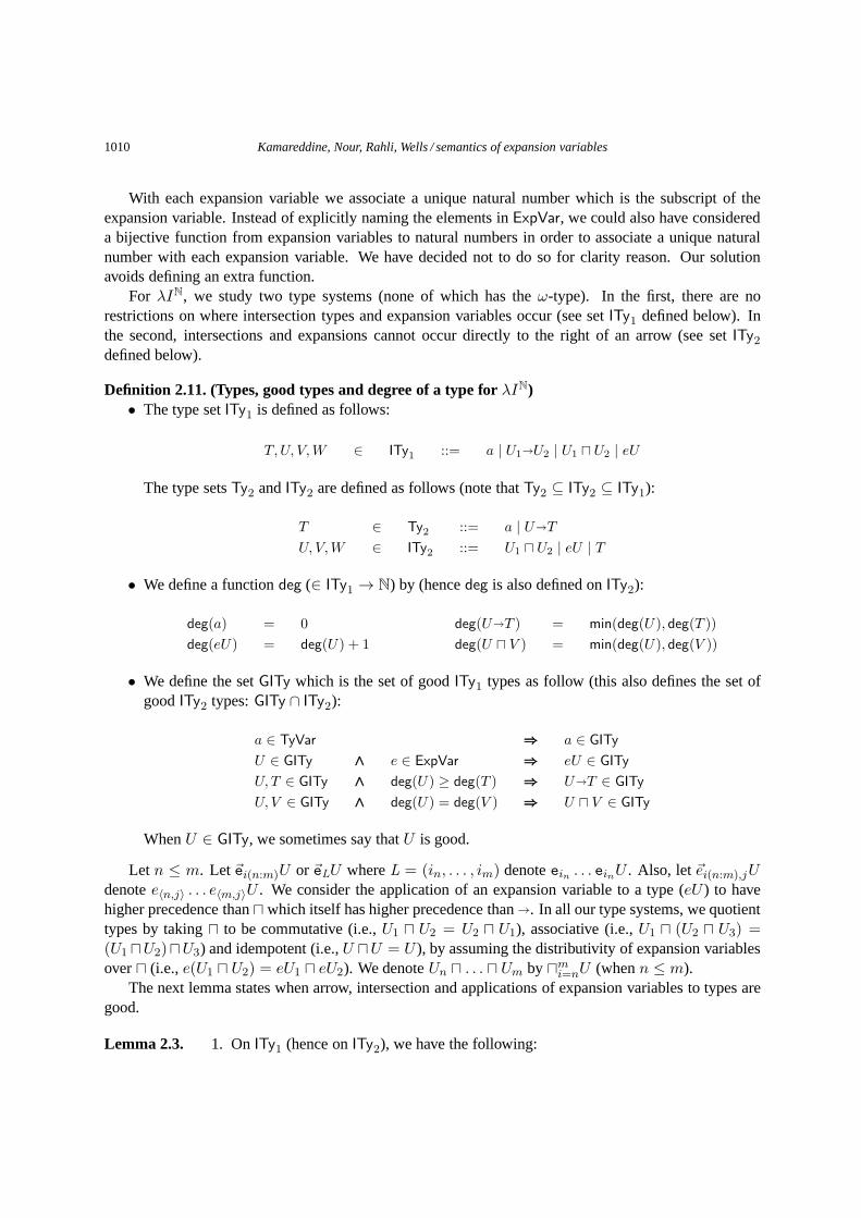
1010 Kamareddine, Nour, Rahli, Wells / semantics of expansion variables
With each expansion variable we associate a unique natural number which is the subscript of theexpansion variable. Instead of explicitly naming the elements inExpVar, we could also have considereda bijective function from expansion variables to natural numbers in order to associate a unique naturalnumber with each expansion variable. We have decided not to do so for clarity reason. Our solutionavoids defining an extra function.
For λIN, we study two type systems (none of which has theω-type). In the first, there are norestrictions on where intersection types and expansion variables occur (see setITy1 defined below). Inthe second, intersections and expansions cannot occur directly to the right of an arrow (see setITy2defined below).
Definition 2.11. (Types, good types and degree of a type forλIN)• The type setITy1 is defined as follows:
T, U, V,W ∈ ITy1 ::= a | U1�U2 | U1 ⊓ U2 | eU
The type setsTy2 andITy2 are defined as follows (note thatTy2 ⊆ ITy2 ⊆ ITy1):
T ∈ Ty2 ::= a | U�T
U, V,W ∈ ITy2 ::= U1 ⊓ U2 | eU | T
• We define a functiondeg (∈ ITy1 → N) by (hencedeg is also defined onITy2):
deg(a) = 0
deg(eU) = deg(U) + 1
deg(U�T ) = min(deg(U), deg(T ))
deg(U ⊓ V ) = min(deg(U), deg(V ))
• We define the setGITy which is the set of goodITy1 types as follow (this also defines the set ofgoodITy2 types:GITy ∩ ITy2):
a ∈ TyVar ⇒⇒⇒ a ∈ GITy
U ∈ GITy ∧∧∧ e ∈ ExpVar ⇒⇒⇒ eU ∈ GITy
U, T ∈ GITy ∧∧∧ deg(U) ≥ deg(T ) ⇒⇒⇒ U�T ∈ GITy
U, V ∈ GITy ∧∧∧ deg(U) = deg(V ) ⇒⇒⇒ U ⊓ V ∈ GITy
WhenU ∈ GITy, we sometimes say thatU is good.
Let n ≤ m. Let~ei(n:m)U or~eLU whereL = (in, . . . , im) denoteein . . . einU . Also, let~ei(n:m),jU
denotee〈n,j〉 . . . e〈m,j〉U . We consider the application of an expansion variable to a type (eU ) to havehigher precedence than⊓ which itself has higher precedence than�. In all our type systems, we quotienttypes by taking⊓ to be commutative (i.e.,U1 ⊓ U2 = U2 ⊓ U1), associative (i.e.,U1 ⊓ (U2 ⊓ U3) =(U1 ⊓U2)⊓U3) and idempotent (i.e.,U ⊓U = U ), by assuming the distributivity of expansion variablesover⊓ (i.e.,e(U1 ⊓ U2) = eU1 ⊓ eU2). We denoteUn ⊓ . . . ⊓ Um by ⊓m
i=nU (whenn ≤ m).The next lemma states when arrow, intersection and applications of expansion variables to types are
good.
Lemma 2.3. 1. OnITy1 (hence onITy2), we have the following:
Kamareddine, Nour, Rahli, Wells / semantics of expansion variables 1011
(a) (U, T ∈ GITy anddeg(U) ≥ deg(T )) iff U�T ∈ GITy.
(b) (U, V ∈ GITy anddeg(U) = deg(V )) iff U ⊓ V ∈ GITy.
(c) U ∈ GITy iff eU ∈ GITy.
2. OnITy2, we have in addition the following:
(a) If T ∈ Ty2 thendeg(T ) = 0.
(b) If deg(U) = n thenU is of the form⊓mi=1~ej(1:n),iVi such thatm ≥ 1 and∃i ∈ {1, . . . ,m}. Vi ∈
Ty2.
(c) If U ∈ GITy anddeg(U) = n thenU is of the form⊓mi=1~ej(1:n),iTi such thatm ≥ 1 and
∀i ∈ {1, . . . ,m}. Ti ∈ Ty2 ∩ GITy.
(d) U, T ∈ GITy iff U�T ∈ GITy (in ITy2 andITy3).
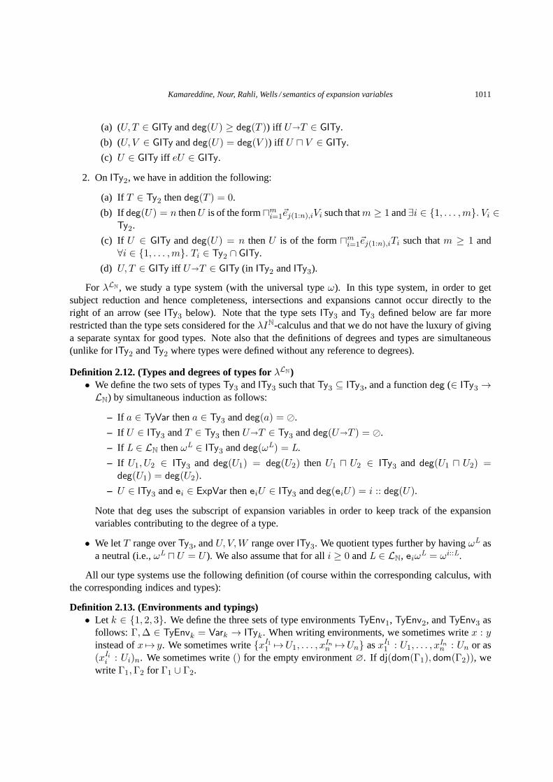
For λLN , we study a type system (with the universal typeω). In this type system, in order to getsubject reduction and hence completeness, intersections and expansions cannot occur directly to theright of an arrow (seeITy3 below). Note that the type setsITy3 andTy3 defined below are far morerestricted than the type sets considered for theλIN-calculus and that we do not have the luxury of givinga separate syntax for good types. Note also that the definitions of degrees and types are simultaneous(unlike for ITy2 andTy2 where types were defined without any reference to degrees).
Definition 2.12. (Types and degrees of types forλLN)• We define the two sets of typesTy3 andITy3 such thatTy3 ⊆ ITy3, and a functiondeg (∈ ITy3 →
LN) by simultaneous induction as follows:
– If a ∈ TyVar thena ∈ Ty3 anddeg(a) = ⊘.
– If U ∈ ITy3 andT ∈ Ty3 thenU�T ∈ Ty3 anddeg(U�T ) = ⊘.
– If L ∈ LN thenωL ∈ ITy3 anddeg(ωL) = L.
– If U1, U2 ∈ ITy3 and deg(U1) = deg(U2) thenU1 ⊓ U2 ∈ ITy3 and deg(U1 ⊓ U2) =deg(U1) = deg(U2).
– U ∈ ITy3 andei ∈ ExpVar theneiU ∈ ITy3 anddeg(eiU) = i :: deg(U).
Note thatdeg uses the subscript of expansion variables in order to keep track of the expansionvariables contributing to the degree of a type.
• We letT range overTy3, andU, V,W range overITy3. We quotient types further by havingωL asa neutral (i.e.,ωL ⊓ U = U ). We also assume that for alli ≥ 0 andL ∈ LN, eiωL = ωi::L.
All our type systems use the following definition (of course within the corresponding calculus, withthe corresponding indices and types):
Definition 2.13. (Environments and typings)• Let k ∈ {1, 2, 3}. We define the three sets of type environmentsTyEnv1, TyEnv2, andTyEnv3 as
follows: Γ,∆ ∈ TyEnvk = Vark → ITyk. When writing environments, we sometimes writex : yinstead ofx 7→ y. We sometimes write{xI11 7→U1, . . . , x
Inn 7→Un} asxI11 : U1, . . . , x
Inn : Un or as
(xIii : Ui)n. We sometimes write() for the empty environment∅. If dj(dom(Γ1), dom(Γ2)), wewrite Γ1,Γ2 for Γ1 ∪ Γ2.

1012 Kamareddine, Nour, Rahli, Wells / semantics of expansion variables
• We say thatΓ1 andΓ2 are joinable and writeΓ1 ⋄ Γ2 iff (∀xI1 ∈ dom(Γ1). xI2 ∈ dom(Γ2) ⇒⇒⇒
I1 = I2).
• We say thatΓ is OK and writeok(Γ) iff ∀xI ∈ dom(Γ). deg(Γ(xI )) = I .
• Let Γ1 = Γ′1 ⊎ Γ′′
1 andΓ2 = Γ′2 ⊎ Γ′′
2 such thatdj(dom(Γ′′1), dom(Γ′′
2)), dom(Γ′1) = dom(Γ′
2),and∀xI ∈ dom(Γ′
1). deg(Γ′1(x
I )) = deg(Γ′2(x
I )). We denoteΓ1 ⊓ Γ2 the type environment{xI 7→Γ′
1(xI )⊓Γ′
2(xI ) | xI ∈ dom(Γ′
1)}∪Γ′′1∪Γ
′′2. Note thatdom(Γ1⊓Γ2) = dom(Γ1)∪dom(Γ2)
and that, on environments,⊓ is commutative, associative and idempotent.
• In λIN (i.e., onTyEnv1 andTyEnv2), we define the set of good type environments as follows:GTyEnv = {Γ | ∀xI ∈ dom(Γ). Γ(xI ) ∈ GITy}. If Γ = (xni
i : Ui)m then letdeg(Γ) =min(n1, . . . , nm, deg(U1), . . . , deg(Um)). Let eΓ = {xn+1 7→ eΓ(xn) | xn ∈ dom(Γ)}. Soe(Γ1 ⊓ Γ2) = eΓ1 ⊓ eΓ2.
• In λLN (i.e., onTyEnv3), if M ∈ M3 and fv(M) = {xL1
1 , . . . , xLnn } then letenvøM be the type
environment(xLi
i : ωLi)n. For all ej ∈ ExpVar, let ejΓ = {xj::L 7→ ejΓ(xL) | xL ∈ dom(Γ)}.
Note thate(Γ1 ⊓ Γ2) = eΓ1 ⊓ eΓ2. If Γ = (xLi
i : Ui)n ands = {L | ∀i ∈ {1, . . . , n}. L �Li ∧ L � deg(Ui)} thendeg(Γ) = L such thatL ∈ s and∀L′ ∈ s. L′ � L.
As we did for terms, we decrease the indexes of types and environments.
Definition 2.14. (Degree decreasing inλIN)• If deg(U) > 0 then we inductively define the typeU− as follows:
(U1 ⊓ U2)− = U1
− ⊓ U2− (eU)− = U
If deg(U) ≥ n then we inductively define the typeU−n as follows:
U−0 = U U−(n+1) = (U−n)−
• If deg(Γ) > 0 then letΓ− = {xn−1 7→Γ(xn)− | xn ∈ dom(Γ)}.
If deg(Γ) ≥ n then we inductively define the typeΓ−n as follows:
Γ−0 = Γ Γ−(n+1) = (Γ−n)−.
Definition 2.15. (Degree decreasing inλLN)1. If deg(U) � L thenU−L is inductively defined as follows:
U−⊘ = U (U1 ⊓ U2)−i::L′
= U−i::L′
1 ⊓ U−i::L′
2 (eiU)−i::L′
= U−L′
We writeU−i instead ofU−(i).
2. If Γ = (xLi
i : Ui)m anddeg(Γ) � L then by definition∀i ∈ {1, . . . ,m}. Li = L :: L′i ∧ L �
deg(Ui), and we defineΓ−L = (xL′i : U−L
i )m. We writeΓ−i instead ofΓ−(i).
Kamareddine, Nour, Rahli, Wells / semantics of expansion variables 1013
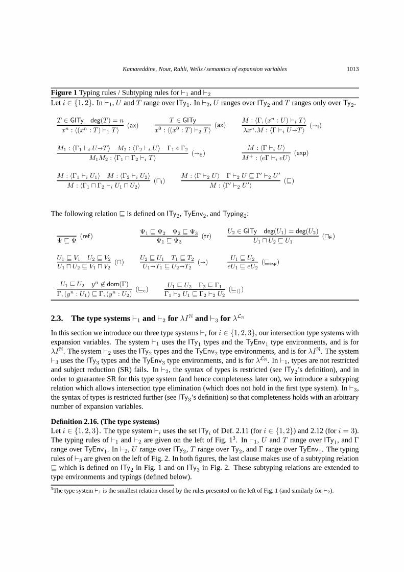
Figure 1 Typing rules / Subtyping rules for⊢1 and⊢2
Let i ∈ {1, 2}. In ⊢1, U andT range overITy1. In ⊢2, U ranges overITy2 andT ranges only overTy2.
T ∈ GITy deg(T ) = n
xn : 〈(xn : T ) ⊢1 T 〉(ax)
T ∈ GITy
x0 : 〈(x0 : T ) ⊢2 T 〉(ax)
M : 〈Γ, (xn : U) ⊢i T 〉
λxn.M : 〈Γ ⊢i U�T 〉(�I)
M1 : 〈Γ1 ⊢i U�T 〉 M2 : 〈Γ2 ⊢i U〉 Γ1 ⋄ Γ2
M1M2 : 〈Γ1 ⊓ Γ2 ⊢i T 〉(�E)
M : 〈Γ ⊢i U〉
M+ : 〈eΓ ⊢i eU〉(exp)
M : 〈Γ1 ⊢i U1〉 M : 〈Γ2 ⊢i U2〉
M : 〈Γ1 ⊓ Γ2 ⊢i U1 ⊓ U2〉(⊓I)
M : 〈Γ ⊢2 U〉 Γ ⊢2 U ⊑ Γ′ ⊢2 U ′
M : 〈Γ′ ⊢2 U ′〉(⊑)
The following relation⊑ is defined onITy2, TyEnv2, andTyping2:
Ψ ⊑ Ψ(ref)
Ψ1 ⊑ Ψ2 Ψ2 ⊑ Ψ3
Ψ1 ⊑ Ψ3(tr)
U2 ∈ GITy deg(U1) = deg(U2)
U1 ⊓ U2 ⊑ U1(⊓E)
U1 ⊑ V1 U2 ⊑ V2
U1 ⊓ U2 ⊑ V1 ⊓ V2(⊓)
U2 ⊑ U1 T1 ⊑ T2
U1�T1 ⊑ U2�T2(�)
U1 ⊑ U2
eU1 ⊑ eU2(⊑exp)
U1 ⊑ U2 yn 6∈ dom(Γ)
Γ, (yn : U1) ⊑ Γ, (yn : U2)(⊑c)
U1 ⊑ U2 Γ2 ⊑ Γ1
Γ1 ⊢2 U1 ⊑ Γ2 ⊢2 U2(⊑〈〉)
2.3. The type systems⊢1 and ⊢2 for λIN and ⊢3 for λLN
In this section we introduce our three type systems⊢i for i ∈ {1, 2, 3}, our intersection type systems withexpansion variables. The system⊢1 uses theITy1 types and theTyEnv1 type environments, and is forλIN. The system⊢2 uses theITy2 types and theTyEnv2 type environments, and is forλIN. The system⊢3 uses theITy3 types and theTyEnv3 type environments, and is forλLN . In ⊢1, types are not restrictedand subject reduction (SR) fails. In⊢2, the syntax of types is restricted (seeITy2’s definition), and inorder to guarantee SR for this type system (and hence completeness later on), we introduce a subtypingrelation which allows intersection type elimination (which does not hold in the first type system). In⊢3,the syntax of types is restricted further (seeITy3’s definition) so that completeness holds with an arbitrarynumber of expansion variables.
Definition 2.16. (The type systems)Let i ∈ {1, 2, 3}. The type system⊢i uses the setITyi of Def. 2.11 (fori ∈ {1, 2}) and 2.12 (fori = 3).The typing rules of⊢1 and⊢2 are given on the left of Fig. 13. In ⊢1, U andT range overITy1, andΓrange overTyEnv1. In ⊢2, U range overITy2, T range overTy2, andΓ range overTyEnv1. The typingrules of⊢3 are given on the left of Fig. 2. In both figures, the last clausemakes use of a subtyping relation⊑ which is defined onITy2 in Fig. 1 and onITy3 in Fig. 2. These subtyping relations are extended totype environments and typings (defined below).
3The type system⊢1 is the smallest relation closed by the rules presented on theleft of Fig. 1 (and similarly for⊢2).
1014 Kamareddine, Nour, Rahli, Wells / semantics of expansion variables
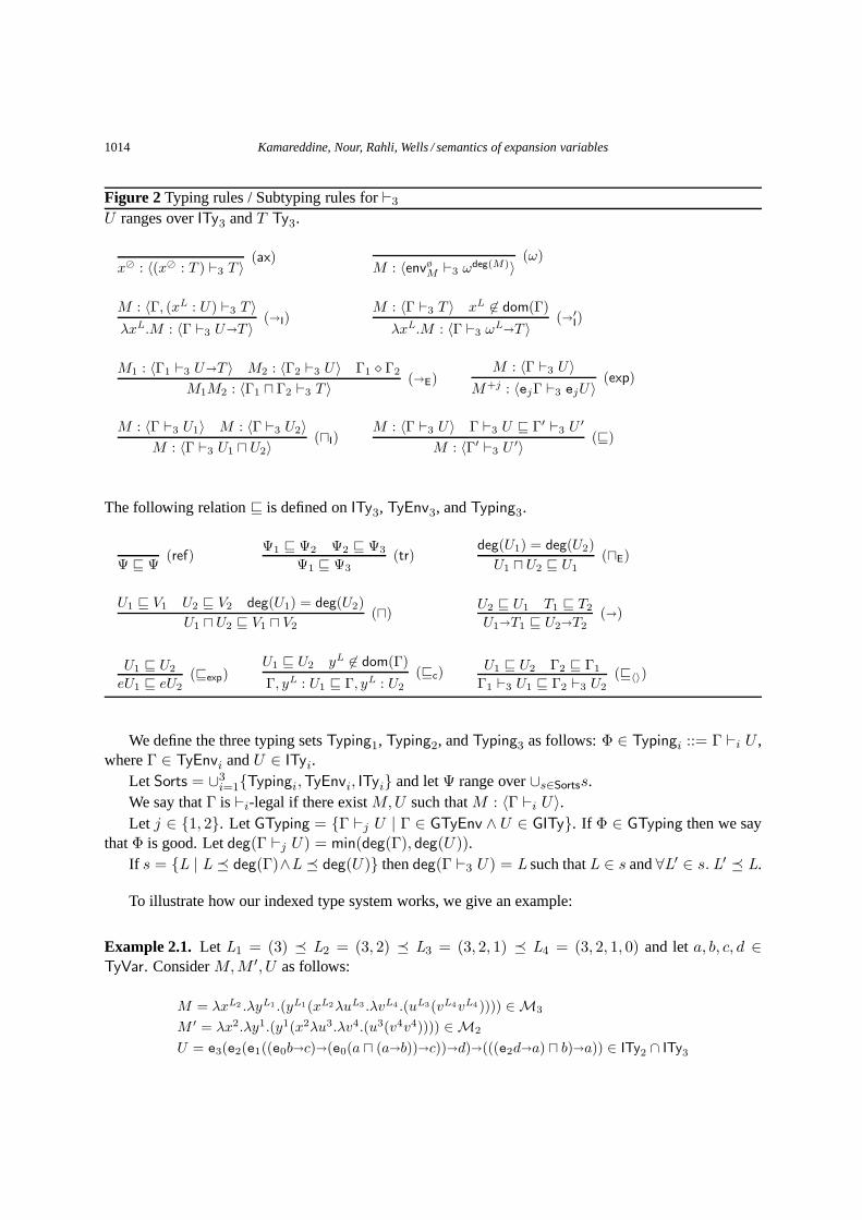
Figure 2 Typing rules / Subtyping rules for⊢3
U ranges overITy3 andT Ty3.
x⊘ : 〈(x⊘ : T ) ⊢3 T 〉(ax)
M : 〈envøM ⊢3 ωdeg(M)〉(ω)
M : 〈Γ, (xL : U) ⊢3 T 〉
λxL.M : 〈Γ ⊢3 U�T 〉(�I)
M : 〈Γ ⊢3 T 〉 xL 6∈ dom(Γ)
λxL.M : 〈Γ ⊢3 ωL�T 〉(�′
I)
M1 : 〈Γ1 ⊢3 U�T 〉 M2 : 〈Γ2 ⊢3 U〉 Γ1 ⋄ Γ2
M1M2 : 〈Γ1 ⊓ Γ2 ⊢3 T 〉(�E)
M : 〈Γ ⊢3 U〉
M+j : 〈ejΓ ⊢3 ejU〉(exp)
M : 〈Γ ⊢3 U1〉 M : 〈Γ ⊢3 U2〉
M : 〈Γ ⊢3 U1 ⊓ U2〉(⊓I)
M : 〈Γ ⊢3 U〉 Γ ⊢3 U ⊑ Γ′ ⊢3 U ′
M : 〈Γ′ ⊢3 U ′〉(⊑)
The following relation⊑ is defined onITy3, TyEnv3, andTyping3.
Ψ ⊑ Ψ(ref)
Ψ1 ⊑ Ψ2 Ψ2 ⊑ Ψ3
Ψ1 ⊑ Ψ3(tr)
deg(U1) = deg(U2)
U1 ⊓ U2 ⊑ U1(⊓E)
U1 ⊑ V1 U2 ⊑ V2 deg(U1) = deg(U2)
U1 ⊓ U2 ⊑ V1 ⊓ V2(⊓)
U2 ⊑ U1 T1 ⊑ T2
U1�T1 ⊑ U2�T2(�)
U1 ⊑ U2
eU1 ⊑ eU2(⊑exp)
U1 ⊑ U2 yL 6∈ dom(Γ)
Γ, yL : U1 ⊑ Γ, yL : U2
(⊑c)U1 ⊑ U2 Γ2 ⊑ Γ1
Γ1 ⊢3 U1 ⊑ Γ2 ⊢3 U2(⊑〈〉)
We define the three typing setsTyping1, Typing2, andTyping3 as follows:Φ ∈ Typingi ::= Γ ⊢i U ,whereΓ ∈ TyEnvi andU ∈ ITyi.
Let Sorts = ∪3i=1{Typingi,TyEnvi, ITyi} and letΨ range over∪s∈Sortss.
We say thatΓ is ⊢i-legal if there existM,U such thatM : 〈Γ ⊢i U〉.Let j ∈ {1, 2}. LetGTyping = {Γ ⊢j U | Γ ∈ GTyEnv ∧ U ∈ GITy}. If Φ ∈ GTyping then we say
thatΦ is good. Letdeg(Γ ⊢j U) = min(deg(Γ), deg(U)).If s = {L | L � deg(Γ)∧L � deg(U)} thendeg(Γ ⊢3 U) = L such thatL ∈ s and∀L′ ∈ s. L′ � L.
To illustrate how our indexed type system works, we give an example:
Example 2.1. Let L1 = (3) � L2 = (3, 2) � L3 = (3, 2, 1) � L4 = (3, 2, 1, 0) and leta, b, c, d ∈TyVar. ConsiderM,M ′, U as follows:
M = λxL2 .λyL1 .(yL1(xL2λuL3 .λvL4 .(uL3(vL4vL4)))) ∈ M3
M ′ = λx2.λy1.(y1(x2λu3.λv4.(u3(v4v4)))) ∈ M2
U = e3(e2(e1((e0b�c)�(e0(a ⊓ (a�b))�c))�d)�(((e2d�a) ⊓ b)�a)) ∈ ITy2 ∩ ITy3
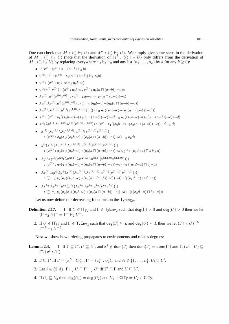
Kamareddine, Nour, Rahli, Wells / semantics of expansion variables 1015
One can check thatM : 〈() ⊢3 U〉 andM ′ : 〈() ⊢2 U〉. We simply give some steps in the derivationof M : 〈() ⊢3 U〉 (note that the derivation ofM ′ : 〈() ⊢2 U〉 only differs from the derivation ofM : 〈() ⊢3 U〉 by replacing everywhere⊢3 by ⊢2 and any list(n1, . . . , nk) by k for anyk ≥ 0):
• v⊘v⊘ : 〈v⊘ : a ⊓ (a�b) ⊢3 b〉
• v(0)v(0) : 〈v(0) : e0(a ⊓ (a�b)) ⊢3 e0b〉
• u⊘ : 〈u⊘ : e0b�c ⊢3 e0b�c〉
• u⊘(v(0)v(0)) : 〈u⊘ : e0b�c, v(0) : e0(a ⊓ (a�b)) ⊢3 c〉
• λv(0).u⊘(v(0)v(0)) : 〈u⊘ : e0b�c ⊢3 e0(a ⊓ (a�b))�c〉
• λu⊘.λv(0).u⊘(v(0)v(0)) : 〈() ⊢3 (e0b�c)�(e0(a ⊓ (a�b))�c)〉
• λu(1).λv(1,0).u(1)(v(1,0)v(1,0)) : 〈() ⊢3 e1((e0b�c)�(e0(a ⊓ (a�b))�c))〉
• x⊘ : 〈x⊘ : e1((e0b�c)�(e0(a ⊓ (a�b))�c))�d ⊢3 e1((e0b�c)�(e0(a ⊓ (a�b))�c))�d〉
• x⊘(λu(1).λv(1,0).u(1)(v(1,0)v(1,0))) : 〈x⊘ : e1((e0b�c)�(e0(a ⊓ (a�b))�c))�d ⊢3 d〉
• x(2)(λu(2,1).λv(2,1,0).u(2,1)(v(2,1,0)v(2,1,0)))
: 〈x(2) : e2(e1((e0b�c)�(e0(a ⊓ (a�b))�c))�d) ⊢3 e2d〉
• y⊘(x(2)(λu(2,1).λv(2,1,0).u(2,1)(v(2,1,0)v(2,1,0))))
: 〈x(2) : e2(e1((e0b�c)�(e0(a ⊓ (a�b))�c))�d), y⊘ : (e2d�a) ⊓ b ⊢3 a〉
• λy⊘.(y⊘(x(2)(λu(2,1).λv(2,1,0).u(2,1)(v(2,1,0)v(2,1,0)))))
: 〈x(2) : e2(e1((e0b�c)�(e0(a ⊓ (a�b))�c))�d) ⊢3 ((e2d�a) ⊓ b)�a〉
• λx(2).λy⊘.(y⊘(x(2)(λu(2,1).λv(2,1,0).u(2,1)(v(2,1,0)v(2,1,0)))))
: 〈() ⊢3 e2(e1((e0b�c)�(e0(a ⊓ (a�b))�c))�d)�(((e2d�a) ⊓ b)�a)〉
• λxL2 .λyL1 .(yL1(xL2(λuL3 .λvL4 .uL3(vL4vL4))))
: 〈() ⊢3 e3(e2(e1((e0b�c)�(e0(a ⊓ (a�b))�c))�d)�(((e2d�a) ⊓ b)�a))〉
Let us now define our decreasing functions on theTyping2.
Definition 2.17. 1. If U ∈ ITy2 andΓ ∈ TyEnv2 such thatdeg(Γ) > 0 anddeg(U) > 0 then we let(Γ ⊢2 U)− = Γ− ⊢2 U
−.
2. If U ∈ ITy3 andΓ ∈ TyEnv3 such thatdeg(Γ) � L anddeg(U) � L then we let(Γ ⊢3 U)−L =Γ−L ⊢3 U
−L.
Next we show how ordering propagates to environments and relates degrees:
Lemma 2.4. 1. If Γ ⊑ Γ′, U ⊑ U ′, andxI 6∈ dom(Γ) thendom(Γ) = dom(Γ′) andΓ, (xI : U) ⊑Γ′, (xI : U ′).
2. Γ ⊑ Γ′ iff Γ = (xIii : Ui)n, Γ′ = (xIii : U ′i)n and∀i ∈ {1, . . . , n}. Ui ⊑ U ′
i .
3. Letj ∈ {2, 3}. Γ ⊢j U ⊑ Γ′ ⊢j U′ iff Γ′ ⊑ Γ andU ⊑ U ′.
4. If U1 ⊑ U2 thendeg(U1) = deg(U2) andU1 ∈ GITy⇔ U2 ∈ GITy.
1016 Kamareddine, Nour, Rahli, Wells / semantics of expansion variables
5. If Γ1 ⊑ Γ2 thendeg(Γ1) = deg(Γ2).
6. Let j ∈ {2, 3}. The relation⊑ is well defined onITyj × ITyj, on TyEnvj × TyEnvj , and onTypingj × Typingj .
7. If Γ1,Γ2 ∈ TyEnv2 andΓ1 ⊑ Γ2 thenΓ1 ∈ GTyEnv⇔ Γ2 ∈ GTyEnv
Proof:We prove 1. and 2. by induction on the derivationΓ ⊑ Γ′. We prove 3. by induction on the derivationΓ ⊢j U ⊑ Γ′ ⊢j U
′. We prove 4. by induction on the derivationU1 ⊑ U2. We prove 5. by induction onthe derivationΓ1 ⊑ Γ2. We prove 6. by induction on a subtyping derivation. We prove7. by inductionon the derivation ofΓ1 ⊑ Γ2. ⊓⊔
The next theorem states that typings are well defined, that within a typing, degrees are well behavedand that we do not allow weakening.
Theorem 2.3. Let j ∈ {1, 2, 3}. We have:
1. ⊢j is well defined onMj × TyEnvj × ITyj.
2. LetM : 〈Γ ⊢j U〉.
(a) deg(M) = deg(U), ok(Γ), anddom(Γ) = fv(M).
(b) If j 6= 3 thenU ∈ GITy, M ∈ M, Γ ∈ GTyEnv, anddeg(Γ) ≥ deg(M).
(c) If j = 3 thendeg(Γ) � deg(U).
(d) If j = 2 anddeg(U) ≥ k thenM−k : 〈Γ−k ⊢2 U−k〉.
(e) If j = 3 anddeg(U) � K thenM−K : 〈Γ−K ⊢3 U−K 〉.
Proof:We prove 1. and 2. by induction on the derivationM : 〈Γ ⊢j U〉. ⊓⊔
Let us now present admissible typing (and subtyping) rules.
Remark 2.1. 1. The rule
M : 〈Γ1 ⊢3 U1〉 M : 〈Γ2 ⊢3 U2〉
M : 〈Γ1 ⊓ Γ2 ⊢3 U1 ⊓ U2〉(⊓′
I) is admissible
2. The rule
U ∈ GITy deg(U) = n
xn : 〈(xn : U) ⊢2 U〉(ax′)
is admissible
3. The rulexdeg(U) : 〈(xdeg(U) : U) ⊢3 U〉(ax′′)
is admissible
4. The ruleU ⊑ ωdeg(U)(ω′)
is admissible
Let us now present some results concerning theω type and joinability.
Lemma 2.5. 1. If M : 〈Γ ⊢3 U〉 thenΓ ⊑ envøM

Kamareddine, Nour, Rahli, Wells / semantics of expansion variables 1017
2. If dom(Γ) = fv(M) andok(Γ) thenM : 〈Γ ⊢3 ωdeg(M)〉.
3. If i ∈ {1, 2, 3}, M1 : 〈Γ1 ⊢i U1〉 andM2 : 〈Γ2 ⊢i U2〉 thenΓ1 ⋄ Γ2 ⇔M1 ⋄M2.
Proof:
1. LetΓ = (xLi
i : Ui)n wherefv(M) = {xL1
1 , . . . , xLnn } by Theorem 2.3.2a. By Remark 2.1.4,∀i ∈
{1, . . . , n}. Ui ⊑ ωdeg(Ui). By Theorem 2.3.2a,ok(Γ) and therefore∀i ∈ {1, . . . , n}. deg(Ui) =Li. Finally, by Lemma 2.4.2,Γ ⊑ envøM .
2. LetΓ = (xLi
i : Ui)n. Then by hypothesesfv(M) = {xL1
1 , . . . , xLnn } and∀i ∈ {1, . . . , n}. deg(Ui) =
Li. By Remark 2.1.4,∀i ∈ {1, . . . , n}. Ui ⊑ ωLi . By Lemma 2.4.2,Γ ⊑ envøM = (xLi : ωLi)n.Since by rule(ω), M : 〈envøM ⊢3 ω
deg(M)〉, we have by rules(⊑) and(⊑〈〉), M : 〈Γ ⊢3 ωdeg(M)〉.
3. ⇐⇐⇐) Let xI1 ∈ dom(Γ1) andxI2 ∈ dom(Γ2) then by Theorem 2.3.2a,xI1 ∈ fv(M1) andxI2 ∈fv(M2). BecauseM1 ⋄ M2, then I1 = I2 and thereforeΓ1 ⋄ Γ2. ⇒⇒⇒) Let xI1 ∈ fv(M1) andxI2 ∈ fv(M2) then by Theorem 2.3.2a,xI1 ∈ dom(Γ1) andxI2 ∈ dom(Γ2). BecauseΓ1 ⋄Γ2, thenI1 = I2 and thereforeM1 ⋄M2.
⊓⊔
2.4. Subject reduction and expansion properties of our typesystems
2.4.1. Subject reduction and expansion properties for⊢1 and ⊢2
Now we list the generation lemmas for⊢1 and⊢2 (for proofs see the expanded version of this article [22]).
Lemma 2.6. (Generation for⊢1)1. If xn : 〈Γ ⊢1 T 〉 thenΓ = (xn : T ).
2. If λxn.M : 〈Γ ⊢1 T1�T2〉 thenM : 〈Γ, xn : T1 ⊢1 T2〉.
3. If MN : 〈Γ ⊢1 T 〉 anddeg(T ) = m thenΓ = Γ1 ⊓ Γ2, T = ⊓ni=1~ej(1:m),iTi, n ≥ 1, M : 〈Γ1 ⊢1
⊓ni=1~ej(1:m),i(T
′i�Ti)〉 andN : 〈Γ2 ⊢1 ⊓
ni=1~ej(1:m),iT
′i 〉.
Lemma 2.7. (Generation for⊢2)1. If xn : 〈Γ ⊢2 U〉 thenΓ = (xn : V ) whereV ⊑ U .
2. If λxn.M : 〈Γ ⊢2 U〉 and deg(U) = m thenU = ⊓ki=1~ej(1:m),i(Vi�Ti) wherek ≥ 1 and
∀i ∈ {1, . . . , k}. M : 〈Γ, xn : ~ej(1:m),iVi ⊢2 ~ej(1:m),iTi〉.
3. If MN : 〈Γ ⊢2 U〉 anddeg(U) = m thenU = ⊓ki=1~ej(1:m),iTi wherek ≥ 1, Γ = Γ1 ⊓ Γ2,
M : 〈Γ1 ⊢2 ⊓ki=1~ej(1:m),i(Ui�Ti)〉, andN : 〈Γ2 ⊢2 ⊓
ki=1~ej(1:m),iUi〉.
We also show that noβ-redexes are blocked in a typable term.
Remark 2.2. (Noβ-redexes are blocked in typable terms)Let i ∈ {1, 2} andM : 〈Γ ⊢i U〉. If (λxn.M1)M2 is a subterm ofM thendeg(M2) = n and hence(λxn.M1)M2 _β M1[x
n := M2].
1018 Kamareddine, Nour, Rahli, Wells / semantics of expansion variables
Lemma 2.8. (Substitution for⊢2)If M : 〈Γ, xI : U ⊢2 V 〉, N : 〈∆ ⊢2 U〉 andM ⋄N thenM [xI := N ] : 〈Γ ⊓∆ ⊢2 V 〉.
Proof:By induction on the derivationM : 〈Γ, xI : U ⊢2 V 〉. ⊓⊔
Lemma 2.9. (Substitution and Subjectβ-reduction fails for ⊢1)Let a, b, c be different type variables. We have:
1. (λx0.x0x0)(y0z0) _β (y0z0)(y0z0).
2. x0x0 : 〈x0 : (a�c) ⊓ a ⊢1 c〉.
3. (λx0.x0x0)(y0z0) : 〈y0 : b�((a�c) ⊓ a), z0 : b ⊢1 c〉.
4. It is not possible that(y0z0)(y0z0) : 〈y0 : b�((a�c) ⊓ a), z0 : b ⊢1 c〉.
Hence, the substitution and subjectβ-reduction lemmas fail for⊢1.
Proof:1., 2., and 3. are easy.
For 4., assume(y0z0)(y0z0) : 〈y0 : b�((a�c) ⊓ a), z0 : b ⊢1 c〉. By Lemma 2.6.3 twice, Theo-rem 2.3 and Lemma 2.6.1:
• y0z0 : 〈y0 : b�((a�c) ⊓ a), z0 : b ⊢1 ⊓ni=1(Ti�c)〉 andn ≥ 1.
• y0 : 〈y0 : b�((a�c) ⊓ a) ⊢1 ⊓ni=1T
′i�Ti�c〉.
• ⊓ni=1T
′i�Ti�c = b�((a�c) ⊓ a).
Hence, for somei ∈ {1, . . . , n}, b = T ′i andTi�c = (a�c) ⊓ a which is absurd. ⊓⊔
Nevertheless, we show thatβ subject reduction and expansion hold in⊢2. This will be used in theproof of completeness (more specifically in Lemma 3.6 which is the basis of the completeness Theo-rem 3.1).
Lemma 2.10. (Subject reduction and expansion for⊢2 w.r.t. β)1. If M : 〈Γ ⊢2 U〉 andM _∗
β N thenN : 〈Γ ⊢2 U〉.
2. If N : 〈Γ ⊢2 U〉 andM _∗β N thenM : 〈Γ ⊢2 U〉.
2.4.2. Subject reduction and expansion properties for⊢3
Now we list the generation lemmas for⊢3 (for proofs see the expanded version of this article [22]).
Lemma 2.11. (Generation for⊢3)1. If xL : 〈Γ ⊢3 U〉 thenΓ = (xL : V ) andV ⊑ U .
2. If λxL.M : 〈Γ ⊢3 U〉, xL ∈ fv(M) anddeg(U) = K thenU = ωK or U = ⊓pi=1~eK(Vi�Ti)
wherep ≥ 1 and∀i ∈ {1, . . . , p}. M : 〈Γ, xL : ~eKVi ⊢3 ~eKTi〉.
Kamareddine, Nour, Rahli, Wells / semantics of expansion variables 1019
3. If λxL.M : 〈Γ ⊢3 U〉, xL 6∈ fv(M) anddeg(U) = K thenU = ωK or U = ⊓pi=1~eK(Vi�Ti)
wherep ≥ 1 and∀i ∈ {1, . . . , p}. M : 〈Γ ⊢3 ~eKTi〉.
4. If MxL : 〈Γ, (xL : U) ⊢3 T 〉 andxL 6∈ fv(M), thenM : 〈Γ ⊢3 U�T 〉.
Proof:1. By induction on the derivationxL : 〈Γ ⊢3 U〉. 2. By induction on the derivationλxL.M : 〈Γ ⊢3 U〉.3. Same proof as that of 2. 4. By induction on the derivationMxL : 〈Γ, xL : U ⊢3 T 〉. ⊓⊔
Lemma 2.12. (Substitution for⊢3)If M : 〈Γ, xL : U ⊢3 V 〉, N : 〈∆ ⊢3 U〉 andM ⋄N thenM [xL := N ] : 〈Γ ⊓∆ ⊢3 V 〉.
Proof:By induction on the derivationM : 〈Γ, xL : U ⊢3 V 〉. ⊓⊔
Since⊢3 does not allow weakening, we need the next definition since when a term is reduced, it maylose some of its free variables and hence will need to be typedin a smaller environment.
Definition 2.18. LetΓ↾s stand fors⊳ Γ. We writeΓ↾M instead ofΓ↾fv(M).
Now we are ready to prove the main result of this section:
Theorem 2.4. (Subject reduction for⊢3)If M : 〈Γ ⊢3 U〉 andM _∗
βη N thenN : 〈Γ↾N ⊢3 U〉.
Proof:By induction on the reductionM _∗
βη N . ⊓⊔
Corollary 2.1. 1. If M : 〈Γ ⊢3 U〉 andM _∗β N thenN : 〈Γ↾N ⊢3 U〉.
2. If M : 〈Γ ⊢3 U〉 andM _∗h N thenN : 〈Γ↾N ⊢3 U〉.
The next lemma is needed for expansion.
Lemma 2.13. If M [xL := N ] : 〈Γ ⊢3 U〉, deg(N) = L, xL ∈ fv(M), andM ⋄N then there exist a typeV and two type environmentsΓ1,Γ2 such thatdeg(V ) = L, M : 〈Γ1, x
L : V ⊢3 U〉, N : 〈Γ2 ⊢3 V 〉,andΓ = Γ1 ⊓ Γ2.
Proof:By induction on the derivationM [xL := N ] : 〈Γ ⊢3 U〉. ⊓⊔
Since more free variables might appear in theβ-expansion of a term, the next definition gives apossible enlargement of an environment.
Definition 2.19. Let m ≥ n, Γ = (xLi
i : Ui)n andX = {xL1
1 , . . . , xLmm }. We writeΓ↑X for xL1
1 :
U1, . . . , xLnn : Un, x
Ln+1
n+1 : ωLn+1 , . . . , xLmm : ωLm . If dom(Γ) ⊆ fv(M), we writeΓ↑M instead of
Γ↑fv(M).
1020 Kamareddine, Nour, Rahli, Wells / semantics of expansion variables
We are now ready to establish that subjectβ-expansion holds in⊢3 (Theorem. 2.5) and that subjectη-expansion fails (Lemma 2.14).
Theorem 2.5. (Subjectβ-expansion holds in⊢3)If N : 〈Γ ⊢3 U〉 andM _∗
β N thenM : 〈Γ↑M ⊢3 U〉.
Proof:By induction on the length of the derivationM _∗
β N using the fact that iffv(P ) ⊆ fv(Q) then
(Γ↑P )↑Q = Γ↑Q. ⊓⊔
Corollary 2.2. If N : 〈Γ ⊢3 U〉 andM _∗h N thenM : 〈Γ↑M ⊢3 U〉.
Lemma 2.14. (Subjectη-expansion fails in⊢3)Let a be a type variable and letx 6= y. We have:
1. λy⊘.λx⊘.y⊘x⊘ _η λy⊘.y⊘.
2. λy⊘.y⊘ : 〈() ⊢3 a�a〉.
3. It is not possible that:λy⊘.λx⊘.y⊘x⊘ : 〈() ⊢3 a�a〉. Hence, subjectη-expansion fails in⊢3.
Proof:1. and 2. are easy. For 3., assumeλy⊘.λx⊘.y⊘x⊘ : 〈() ⊢3 a�a〉. By Lemma 2.11.2,λx⊘.y⊘x⊘ :〈(y : a) ⊢3 a〉. Again, by Lemma 2.11.2,a = ω⊘ or there existsn ≥ 1 such thata = ⊓n
i=1(Ui�Ti),absurd. ⊓⊔
3. Realisability semantics and their completeness
3.1. Realisability
Crucial to a realisability semantics is the notion of a saturated set:
Definition 3.1. (Saturated sets)Let i ∈ {1, 2, 3} andM ,M 1,M 2 ⊆ Mi.
1. LetM 1 M 2 = {M ∈ Mi | ∀N ∈ M 1. M ⋄N ⇒⇒⇒ MN ∈ M 2}.
2. LetM 1 ≀M 2 iff ∀M ∈ M 1 M 2. ∃N ∈ M 1. M ⋄N .
3. Forr ∈ {β, βη, h}, let SATr = {M ⊆ Mi | (M _∗r N ∧N ∈ M ) ⇒⇒⇒ M ∈ M }. If M ∈ SATr
then we say thatM is r-saturated.
Saturation is closed under intersection, lifting and arrows:
Lemma 3.1. Let i ∈ {1, 2, 3}, r ∈ {β, βη, h}, andM 1,M 2 ⊆ Mi.
1. If M 1,M 2 arer-saturated sets thenM 1 ∩M 2 is r-saturated.
2. If M 1 ⊆ M2 is r-saturated thenM 1+ is r-saturated.
Kamareddine, Nour, Rahli, Wells / semantics of expansion variables 1021
3. If M 1 ⊆ M3 is r-saturated thenM+i
1 is r-saturated.
4. If M 2 is r-saturated thenM 1 M 2 is r-saturated.
5. If M 1,M 2 ⊆ M2 then(M 1 M 2)+ ⊆ M 1
+ M 2+.
6. If M 1,M 2 ⊆ M3 then(M 1 M )+i ⊆ M+i1 M
+i2 .
7. LetM 1,M 2 ⊆ M2. If M 1+ ≀M 2
+, thenM 1+ M 2
+ ⊆ (M 1 M 2)+.
8. LetM 1,M 2 ⊆ M3. If M+i
1 ≀M+i
2 , thenM+i
1 M+i
2 ⊆ (M 1 M 2)+i.
9. For everyn ∈ N, the setMn is r-saturated.
The interpretations and meanings of types are crucial to a realisability semantics:
Definition 3.2. (Interpretations and meaning of types)Let Var = Var1 ∪ Var2 such thatdj(Var1,Var2) andVar1,Var2 are both countably infinite. Leti ∈{1, 2, 3}.
1. Letx ∈ Vari andI an index. We define the following family of sets:
VARIx = {M ∈ Mi | ∃N1, . . . , Nn ∈ Mi. M = xIN1 . . . Nn}.
2. InλIN, let r = β andI0 = 0. In λLN , let r ∈ {β, βη, h} andI0 = ⊘.
(a) Anri-interpretationI is a function inTyVar → P(MI0i ) such that for alla ∈ TyVar:
I(a) ∈ SATr ∀x ∈ Var1. VARI0x ⊆ I(a) In λIN, I(a) ⊆ M
0
(b) We extendI to ITy1 in case ofλIN and toITy3 in case ofλLN as follows:
In λIN andλLN : I(U1 ⊓ U2) = I(U1) ∩ I(U2) I(U�T ) = I(U) I(T )
In λIN: I(eU) = I(U)+
In λLN : I(eiU) = I(U)+i I(ωL) = ML
3
Let Interpri = {I | I is ari-interpretation}4.
(c) LetU ∈ ITyi. We define[U ]ri , theri-interpretation ofU as follows:
[U ]ri = {M ∈ Mi | closed(M) ∧M ∈⋂
I∈Interpri I(U)}
Because∩ is commutative, associative, idempotent,(M 1 ∩ M 2)+ = M 1
+ ∩ M 2+ in λIN, (M 1 ∩
M 2)+i = M
+i1 ∩M
+i2 in λLN , andI is well defined.
Type interpretations are saturated and interpretations ofgood types contain only good terms.
Lemma 3.2. Let r ∈ {β, βη, h}. Let i ∈ {1, 2, 3}.
1. (a) For allU ∈ ITyi andI ∈ Interpri , we haveI(U) ∈ SATr.
4We effectively define five interpretation setsInterpβ1 , Interpβ2 , Interpβ3 , Interpβη3 , andInterph3

1022 Kamareddine, Nour, Rahli, Wells / semantics of expansion variables
(b) If deg(U) = L andI ∈ Interpr3 then∀x ∈ Var1. VARLx ⊆ I(U) ⊆ ML
3 .
(c) On ITy1 (hence also onITy2), if U ∈ GITy, deg(U) = n, andI ∈ Interpr2 then∀x ∈Var1. x
n ∈ VARnx ⊆ I(U) ⊆ M
n.
2. Let i ∈ {2, 3}. If I ∈ Interpri andU ⊑ V thenI(U) ⊆ I(V ).
Proof:1a . By induction onU using Lemma 3.1. 1b. By induction onU . 1c. By definition,xn ∈ VARn
x. WeproveVARn
x ⊆ I(U) ⊆ Mn by induction onU ∈ GITy. 2. By induction of the derivationU ⊑ V . ⊓⊔
Corollary 3.1. (Meanings of good types consist of good terms)On ITy1 (hence also onITy2), if U ∈ GITy such thatdeg(U) = n then[U ]β2
⊆ Mn.
Proof:By Lemma 3.2.1c, for any interpretationI ∈ Interpβ2, I(U) ⊆ M
n. ⊓⊔
Lemma 3.3. (Soundness of⊢1, ⊢2, and⊢3)Let i ∈ {1, 2, 3}, r ∈ {β, βη, h}, I ∈ Interpri . If M : 〈(x
Ijj : Uj)n ⊢i U〉, ∀j ∈ {1, . . . , n}. Nj ∈
I(Uj), and⋄{M,N1, . . . , Nn} thenM [(xIjj := Nj)n] ∈ I(U).
Proof:By induction on the derivationM : 〈(x
Ijj : Uj)n ⊢i U〉. ⊓⊔
Corollary 3.2. Let r ∈ {β, βη, h} andi ∈ {1, 2, 3}. If M : 〈() ⊢i U〉 thenM ∈ [U ]ri .
Proof:By Lemma 3.3,M ∈ I(U) for anyI ∈ Interpri . By Theorem 2.3,fv(M) = dom(()) = ∅ and henceM is closed. Therefore,M ∈ [U ]ri . ⊓⊔
Lemma 3.4. (The meaning of types is closed under type operations)Let r ∈ {β, βη, h} andj ∈ {1, 2, 3}. The following hold:
1. [eiU ]r3 = [U ]+ir3
and if j 6= 3 then[eU ]rj = [U ]rj+.
2. [U ⊓ V ]rj = [U ]rj ∩ [V ]rj .
3. If U�T ∈ ITy3 then∀I ∈ Interpr3 . I(U) ≀ I(T ).
4. If U�T ∈ GITy then∀I ∈ Interpβ2 . I(U) ≀ I(T ).
5. OnITy1 only (sinceeU�eT 6∈ ITy2), we have: ifU�T ∈ GITy then[e(U�T )]β2= [eU�eT ]β2
.
Proof:1. and 2. are easy.
3. Letdeg(U) = L, M ∈ I(U) I(T ) andx ∈ Var1 such that∀K. xK 6∈ fv(M), henceM ⋄ xL
and by Lemma 3.2,xL ∈ I(U).
Kamareddine, Nour, Rahli, Wells / semantics of expansion variables 1023
4. Let deg(U) = n andM ∈ I(U) I(T ). Takex ∈ Var1 such that∀p. xp 6∈ fv(M). Hence,M ⋄ xn. By Lemma 2.3,U ∈ GITy and by Lemma 3.2,xn ∈ I(U).
5. SinceU�T ∈ GITy then, by Lemma 2.3,U, T ∈ GITy and deg(U) ≥ deg(T ). Again byLemma 2.3,eU, eT ∈ GITy, deg(eU) ≥ deg(eT ) andeU�eT ∈ GITy. Hence by 4.,I(U)+ ≀I(T )+. Thus, by Lemma 3.1.5 and Lemma 3.1.7,∀I ∈ Interpβ2 . I(e(U�T )) = I(eU�eT ).
⊓⊔
Let us now put the realisability semantics in use.
Example 3.1. Let a andb be two distinct type variables inTyVar. We define:
• id0 = a�a andid1 = e1(id0).
• d = (a ⊓ (a�b))�b.
• nat0 = (a�a)�(a�a), nat1 = e1(nat0), andnat′0 = (e1a�a)�(e1a�a).
Moreover, ifM,N are terms andn ∈ N, we define(M)nN by induction onn as follows:(M)0N = N
and(M)m+1N = M((M)mN).We now illustrate our realisability semantics by providingthe meaning of the types defined above:
1. [(a ⊓ b)�a]β1= {M ∈ M
0 | M _∗β λy0.y0}.
2. It is not possible thatλy0.y0 : 〈() ⊢1 (a ⊓ b)�a〉.
3. λy0.y0 : 〈() ⊢2 (a ⊓ b)�a〉.
4. [id0]β3= {M ∈ M⊘
3 | closed(M) ∧M _∗β λy⊘.y⊘}.
5. [id1]β3= {M ∈ M
(1)3 | closed(M) ∧M _∗
β λy(1).y(1)}.
6. [d]β3= {M ∈ M⊘
3 | closed(M) ∧M _∗β λy⊘.y⊘y⊘}.
7. [nat0]β3= {M ∈ M⊘
3 | closed(M)∧(M _∗β λf⊘.f⊘∨(n ≥ 1∧M _∗
β λf⊘.λy⊘.(f⊘)ny⊘))}.
8. [nat1]β3= {M ∈ M
(1)3 | closed(M)∧(M _∗
β λf (1).f (1)∨(n ≥ 1∧M _∗β λf (1).λx(1).(f (1))ny(1)))}.
9. [nat′0]β3= {M ∈ M⊘
3 | closed(M) ∧ (M _∗β λf⊘.f⊘ ∨M _∗
β λf⊘.λy(1).f⊘y(1))}.
3.2. Completeness challenges inλIN
In this document we consider two realisability semantics oftypes involving E-variables. These semanticsare based on a hierarchy of types and terms. Considering how expansions can introduce new substitu-tions, new expansions and an unbound number of new variables(type variables and E-variables), it wasdecided to use a hierarchy on types and terms to give meaningsto expansions to represent the encapsu-lation of types by E-variables. An obvious (and naive) approach is to label types and terms with naturalnumbers. This is the hierarchy we used inλIN. When assigning meanings to types, we ensured that each
1024 Kamareddine, Nour, Rahli, Wells / semantics of expansion variables
use of an E-variable in a typing simply changes the indexes oftypes and terms in the typing and that eachE-variable acted as a kind of capsule that isolates parts of the analysedλ-term in a typing. This capturedthe intuition behind E-variables. However, there are two issues w.r.t. this indexing: it imposes that thetypeω should have all possible indexes (which is impossible5 and hence we eliminatedω from the typesystems forM2) and it implies that the realisability semantics can only becomplete when a single E-variable is used (as we will see in this section). In order to understand the challenges of the semantics ofE-variables withω and the idea behind the hierarchy, we first studied two representative intersection typesystems for theλI-calculus. The restriction toλI (where in every(λx.M) the variablex must occur freein M ) was motivated by not supporting theω type while preserving the intuitive indexes made of singlenatural numbers. For⊢1, the first of these type systems, we showed that subject reduction and hencecompleteness do not hold.
3.2.1. Completeness for⊢1 fails
Remark 3.1. (Failure of completeness for⊢1)Items 1., 2., and 3. of Example 3.1 show that we can not have a completeness result (a converse of thesoundness Lemma 3.3 for closed terms) for⊢1. To type the termλy0.y0 by the type(a⊓ b)�a, we needan elimination rule for⊓ which we do not have in⊢1.
Note that failure of completeness for⊢1 is related to the failure of its subject reduction. So, one mightthink that since⊢2, the second type system forλIN, has subject reduction, its semantics is complete. Thisis not entirely true.
3.2.2. Completeness for⊢2 fails with more than one E-variable
Remark 3.2. (Failure of completeness for⊢2 if more than one E-variable are used)Let a be a type variable,e1 ande2 be two distinct expansion variable, andnat′′0 = (e1a�a)�(e2a�a).Then:
1. λf0.f0 ∈ [nat′′0]β2.
2. it is not possible thatλf0.f0 : 〈() ⊢2 nat′′0〉.
Henceλf0.f0 ∈ [nat′′0 ]β2but λf0.f0 is not typable bynat′′0 and we do not have completeness in the
presence of more than one expansion variable.
However, we will see that we have completeness for⊢2 if only one expansion variable is used.
3.2.3. Completeness for⊢2 with only one E-variable
The problem shown in remark 3.2 comes from the fact that the realisability semantics designed for⊢2
identifies all expansion variables. In order to give a completeness theorem for⊢2 we will, in whatfollows, restrict our system to only one expansion variable. In the rest of this section, we assume that thesetExpVar contains only one expansion variablee1.
5Let us assume that that our type language contains theω type annotated with integers, i.e., of the formωn, then we wouldneede1ωn = ωn+1 ande2ωn = ωn+1, and finally we would havee1ωn = e2ω
n.
Kamareddine, Nour, Rahli, Wells / semantics of expansion variables 1025
The need of one single expansion variable is clear in item 2. of Lemma 3.5 which would fail if we usemore than one expansion variable. For example, ife1 6= e2 then(e1a)− = a = (e2a)
− but e1a 6= e2a.This lemma is crucial for the rest of this section and hence, asingle expansion variable is also crucial.
Lemma 3.5. LetU, V ∈ ITy2 anddeg(U) = deg(V ) > 0.
1. e1U− = U .
2. If U− = V − thenU = V .
Proof:1. is by induction onU . 2. goes as follows: ifU− = V − thene1U− = e1V
− and by 1.,U = V . ⊓⊔
Despite the difference in the number of considered expansion variables in the completeness proofpresented in the current section and the one of Sec. 3.3, bothproofs share some similarities. We stillwrite these two proofs independently to illustrate the method and especially since the proof in the cur-rent section is far simpler. Furthermore, in the current section we only show the completeness of oursemantics w.r.t.β-reduction.
The first step of the proof is to divide{yn | y ∈ Var2} into disjoint subset amongst types of ordern.
Definition 3.3. Let U ∈ ITy2. We define the set of variablesDVarU by induction ondeg(U). Ifdeg(U) = 0 thenDVarU is an infinite set{y0 | y ∈ Var2} such that ifU 6= V anddeg(U) = deg(V ) = 0thendj(DVarU ,DVarV ). If deg(U) = n+ 1 thenDVarU = {yn+1 | yn ∈ DVarU−}.
Our partition ofVar2 allows useful infinite sets containing type environments that will play a crucialrole in one particular type interpretation. These sets and environments are given in the next definition.
Definition 3.4. • Let IPreEnvn = {Lyn, UM | U ∈ ITy2 ∧ deg(U) = n ∧ yn ∈ DVarU} andBPreEnvn =
⋃m≥n IPreEnv
m (where “I” stands for “index” and “B” stands for “bound”). Notethat IPreEnvn andBPreEnvn are not type environments because they are not functions.
• If M ∈ M2 andU ∈ ITy2 then we writeM : 〈BPreEnvn ⊢2 U〉 iff there is a type environmentΓ ⊆ BPreEnvn whereM : 〈Γ ⊢2 U〉.
Now, for everyn, we define the set of the good terms of ordern which contain some free variablexi
wherex ∈ Var1 andi ≥ n.
Definition 3.5. LetOPENn = {M ∈ Mn | xi ∈ fv(M) ∧ x ∈ Var1 ∧ i ≥ n}.
Obviously, ifx ∈ Var1 thenVARnx ⊆ OPENn.
Here is the crucialβ2-interpretationI for the proof of completeness:
Definition 3.6. Let I be theβ2-interpretation defined as follows: for all type variablesa, I(a) = OPEN0∪{M ∈ M0
2 | M : 〈BPreEnv0 ⊢2 a〉}.
The functionI is indeed aβ2-interpretation and the interpretation of a type of ordern contains thegood terms of ordern which are typable in the special environments which are parts of the infinite setsof definition 3.4:
1026 Kamareddine, Nour, Rahli, Wells / semantics of expansion variables
Lemma 3.6. 1. I is aβ2-interpretation, i.e., for alla ∈ TyVar, I(a) is β-saturated and∀x ∈ Var1,VAR0
x ⊆ I(a) ⊆ M0.
2. If U ∈ ITy2∩GITy anddeg(U) = n thenI(U) = OPENn∪{M ∈ Mn | M : 〈BPreEnvn ⊢2 U〉}.
Proof:We prove 1. by first showing thatI(a) is saturated: ifM _∗
β N then if N ∈ OPEN0 we prove that
M ∈ OPEN0 and if N ∈ {M ∈ M02 | M : 〈BPreEnv0 ⊢2 a〉} thenM ∈ {M ∈ M0
2 | M :〈BPreEnv0 ⊢2 a〉}. We then show∀x ∈ Var1. VAR
0x ⊆ I(a) ⊆ M
0. We prove 2. by induction onU ∈ GITy. ⊓⊔
I is used to prove completeness (for the proof see the expandedversion of this article [22])
Theorem 3.1. (Completeness)LetU ∈ ITy2 ∩ GITy such thatdeg(U) = n. The following hold:
1. [U ]β2= {M ∈ M
n | M : 〈() ⊢2 U〉}.
2. [U ]β2is stable by reduction: ifM ∈ [U ]β2
andM _∗β N thenN ∈ [U ]β2
.
3. [U ]β2is stable by expansion: ifN ∈ [U ]β2
andM _∗β N thenM ∈ [U ]β2
.
Proof:The first item follows by Lemmas 3.6 and 3.3. We obtain the second item using subject reduction andthe third one using subject expansion. ⊓⊔
3.3. Completeness forλLN
Having understood the challenges of E-variables and the difficulty of representing the typeω usingnatural numbers as indices for the hierarchy, we moved to thepresentation of indices as sequences ofnatural numbers and we provided our third type system⊢3. We developed a realisability semantics wherewe allow the fullλ-calculus (i.e., where K-redexes are allowed) indexed withlists of natural numbers,an arbitrary (possibly infinite) number of expansion variables and whereω is present, and we showed itssoundness. Now, we show its completeness.
We need the following partition of the set of indexed variables{yL | y ∈ Var2}.
Definition 3.7. • Let ITyL3 = {U ∈ ITy3 | deg(U) = L} andVarL = {xL | x ∈ Var2}.
• We inductively define, for everyU ∈ ITy3, a set of variablesDVarU as follows:
– If deg(U) = ⊘ then:
∗ DVarU is an infinite set of indexed variables of degree⊘.
∗ If U 6= V anddeg(U) = deg(V ) = ⊘ thendj(DVarU ,DVarV ).
∗⋃
U∈ITy⊘3
DVarU = Var⊘.
– If deg(U) = i :: L thenDVarU = {yi::L | yL ∈ DVarU−i}.
Therefore, ifdeg(U) = L thenDVarU = {yL | y⊘ ∈ DVarU−L}.
Kamareddine, Nour, Rahli, Wells / semantics of expansion variables 1027
Let us now provide some simple results concerning theDVarU sets:
Lemma 3.7. 1. If deg(U) � L, deg(V ) � L, andU−L = V −L thenU = V .
2. If deg(U) = L thenDVarU is an infinite subset ofVarL.
3. If U 6= V anddeg(U) = deg(V ) = L thendj(DVarU ,DVarV ).
4.⋃
U∈ITyL3DVarU = VarL.
5. If yL ∈ DVarU thenyi::L ∈ DVareiU .
6. If yi::L ∈ DVarU thenyL ∈ DVarU−i .
Proof:1. goes as follows: ifL = (ni)m then we haveU = en1
. . . enmU′ andV = en1
. . . enmV′; then
U−L = U ′, V −L = V ′ andU ′ = V ′; thusU = V . 2., 3. and 4. are by induction onL and using 1. Weobtain 5. because(eiU)−i = U . 6. is by definition. ⊓⊔
The setVar2 as defined above allows us to give in the next definition usefulinfinite sets containingtype environments that will play a crucial role in one particular type interpretation.
Definition 3.8. • Let L ∈ LN. We denoteIPreEnvL = {LyL, UM | U ∈ ITyL3 ∧ yL ∈ DVarU} andBPreEnvL =
⋃K�L IPreEnvK . Note thatIPreEnvL andBPreEnvL are not type environments
because they are not functions.
• LetL ∈ LN, M ∈ M3 andU ∈ ITy3, we write:
– M : 〈BPreEnvL ⊢3 U〉 iff there exists a type environmentΓ ⊆ BPreEnvL such thatM :〈Γ ⊢3 U〉.
– M : 〈BPreEnvL ⊢∗3 U〉 iff M _∗
βη N andN : 〈BPreEnvL ⊢3 U〉.
Let us now provide some results concerning theBPreEnvL sets:
Lemma 3.8. 1. If Γ ⊆ BPreEnvL thenok(Γ).
2. If Γ ⊆ BPreEnvL theneiΓ ⊆ BPreEnvi::L.
3. If Γ ⊆ BPreEnvi::L thenΓ−i ⊆ BPreEnvL.
4. If Γ1 ⊆ BPreEnvL, Γ2 ⊆ BPreEnvK , andL � K thenΓ1 ⊓ Γ2 ⊆ BPreEnvL.
Proof:1. is by definition. 2. and 3. are by Lemma 3.7. 4. First, by 1.,Γ1⊓Γ2 is well defined. Also,BPreEnvK ⊆BPreEnvL. Let (Γ1 ⊓ Γ2)(x
L′) = U1 ⊓ U2 whereΓ1(x
L′) = U1 andΓ2(x
L′) = U2, thendeg(U1) =
deg(U2) = L′ andxL′∈ DVarU1
∩DVarU2. Hence, by Lemma 3.7.3,U1 = U2 andΓ1⊓Γ2 = Γ1∪Γ2 ⊆
BPreEnvL. ⊓⊔

1028 Kamareddine, Nour, Rahli, Wells / semantics of expansion variables
For everyL ∈ LN, we define the set of terms of degreeL which contain some free variablexK wherex ∈ Var1 andK � L.
Definition 3.9. For everyL ∈ LN, letOPENL = {M ∈ ML3 | xK ∈ fv(M) ∧ x ∈ Var1 ∧K � L}. It
is easy to see that, for everyL ∈ LN andx ∈ Var1, VARL
x ⊆ OPENL.
Let us now provide some results on theOPENL sets:
Lemma 3.9. 1. (OPENL)+i = OPENi::L.
2. If y ∈ Var2 andMyK ∈ OPENL thenM ∈ OPENL.
3. If M ∈ OPENL, M ⋄N , andL � K = deg(N) thenMN ∈ OPENL.
4. If deg(M) = L, L � K, M ⋄N , andN ∈ OPENK thenMN ∈ OPENL.
Proof:Easy using Def. 3.9. ⊓⊔
The crucial interpretationI (the three interpretationsIβη, Iβ , andIh for our three reduction relations)used in the completeness proof is given as follows:
Definition 3.10. 1. Let Iβη be theβη3-interpretation defined by: for all type variablesa, Iβη(a) =OPEN⊘ ∪ {M ∈ M⊘
3 | M : 〈BPreEnv⊘ ⊢∗3 a〉}.
2. Let Iβ be theβ3-interpretation defined by: for all type variablesa, Iβ(a) = OPEN⊘ ∪ {M ∈M⊘
3 | M : 〈BPreEnv⊘ ⊢3 a〉}.
3. Let Ih be theh3-interpretation defined by: for all type variablesa, Ih(a) = OPEN⊘ ∪ {M ∈M⊘
3 | M : 〈BPreEnv⊘ ⊢3 a〉}.
The next crucial lemma shows thatI (the three functionsIβη, Iβ, andIh) is an interpretation andthat the interpretation of a type of orderL contains terms of orderL which are typable in these specialenvironments which are parts of the infinite sets of Def. 3.8.
Lemma 3.10. Let r ∈ {βη, β, h} andr′ ∈ {β, h}.
1. If Ir ∈ Interpr3 anda ∈ TyVar thenIr(a) ∈ SATr and∀x ∈ Var1. VAR⊘x ⊆ Ir(a).
2. If U ∈ ITy3 anddeg(U) = L thenIβη(U) = OPENL ∪ {M ∈ ML3 | M : 〈BPreEnvL ⊢∗
3 U〉}.
3. If U ∈ ITy3 anddeg(U) = L thenIr′(U) = OPENL ∪ {M ∈ ML3 | M : 〈BPreEnvL ⊢3 U〉}.
Proof:We prove the first item by first showing thatIr(a) is saturated: ifM _∗
r N then if N ∈ OPEN⊘ weprove thatM ∈ OPEN⊘ and ifN ∈ {M ∈ M⊘
3 | M : 〈BPreEnv⊘ ⊢∗3 a〉} thenM ∈ {M ∈ M⊘
3 |M : 〈BPreEnv⊘ ⊢∗
3 a〉}. We then show that for allx ∈ Var1, VAR⊘x ⊆ OPEN⊘ ⊆ Ir(a). We prove the
second and third items by induction onU . ⊓⊔
Kamareddine, Nour, Rahli, Wells / semantics of expansion variables 1029
Now, we use this crucialI to establish completeness of our semantics.
Theorem 3.2. (Completeness of⊢3)LetU ∈ ITy3 such thatdeg(U) = L.
1. [U ]βη3 = {M ∈ ML3 | closed(M) ∧M _∗
βη N ∧N : 〈() ⊢3 U〉}.
2. [U ]β3= [U ]h3
= {M ∈ ML3 | M : 〈() ⊢3 U〉}.
3. [U ]βη3 is stable by reduction: ifM ∈ [U ]βη3 andM _βη N thenN ∈ [U ]βη3 .
Proof:
1. LetM ∈ [U ]βη3 . ThenM is closed andM ∈ Iβη(U). By Lemma 3.10.2,M ∈ OPENL ∪ {M ∈ML
3 | M : 〈BPreEnvL ⊢∗3 U〉}. SinceM is closed,M 6∈ OPENL. Hence,M ∈ {M ∈ ML
3 |M : 〈BPreEnvL ⊢∗
3 U〉} and so,M _∗βη N andN : 〈Γ ⊢3 U〉 whereΓ ⊆ BPreEnvL. By
Theorem 2.1.2,N is closed and, by Lemma 2.3.2a,N : 〈() ⊢3 U〉.
Conversely, takeM closed such thatM _∗β N andN : 〈() ⊢3 U〉. Let I ∈ Interpβ3. By
Lemma 3.3,N ∈ I(U). By Lemma 3.2.1,I(U) is βη-saturated. Hence,M ∈ I(U). ThusM ∈ [U ]βη3 .
2. LetM ∈ [U ]β3. ThenM is closed andM ∈ Iβ(U). By Lemma 3.10.3,M ∈ OPENL ∪ {M ∈
ML3 | M : 〈BPreEnvL ⊢3 U〉}. SinceM is closed,M 6∈ OPENL. Hence,M ∈ {M ∈ ML
3 |M : 〈BPreEnvL ⊢3 U〉} and so,M : 〈Γ ⊢3 U〉 whereΓ ⊆ BPreEnvL. By Lemma 2.3.2a,N : 〈() ⊢3 U〉.
Conversely, takeM such thatM : 〈() ⊢3 U〉. By Lemma 2.3.2a,M is closed. LetI ∈ Interpβ3.By Lemma 3.3,M ∈ I(U). ThusM ∈ [U ]β3
.
It is easy to see that[U ]β3= [U ]h3
.
3. Let M ∈ [U ]βη3 andM _βη N . By 1., M is closed,M _∗βη P , andP : 〈() ⊢3 U〉. By
confluence Theorem 2.2, there isQ such thatP _∗βη Q andN _∗
βη Q. By subject reductionTheorem 2.4,Q : 〈() ⊢3 U〉. By Theorem 2.1.2,N is closed and, by 1.,N ∈ [U ]βη3 .
⊓⊔
4. Conclusion and future work
Expansion may be viewed to work like a multi-layered simultaneous substitution. Moreover, expansionis a crucial part of a procedure for calculating principal typings and helps support compositional type in-ference. Because the early definitions of expansion were complicated, expansion variables (E-variables)were introduced to simplify and mechanize expansion. The aim of this document is to give a completesemantics for intersection type systems with expansion variables.
We studied first theλIN-calculus, an indexed version of theλI-calculus. This indexed version wastyped using first a basic intersection type system with expansion variables but without an intersection
1030 Kamareddine, Nour, Rahli, Wells / semantics of expansion variables
elimination rule, and then using an intersection type system with expansion variables and an eliminationrule.
We gave a realisability semantics for both type systems showing that the first type system is notcomplete in the sense that there are types whose semantics isnot the set ofλIN-terms having this type.In particular, we showed thatλy0.y0 is in the semantics of(a ⊓ b)�a but that it is not possible to giveλy0.y0 the type(a ⊓ b)�a in the type system⊢1 (see Example 3.1 in Ch. 3.1). The main reason forthe failure of completeness in the first system is associatedwith the failure of the subject reductionproperty for this first type system. Hence, we moved to the second system which we showed to havethe desirable properties of subject reduction and expansion and strong normalisation. However, for thissecond system, we showed again that completeness fails if weuse more than one expansion variable butthat completeness succeeds if we restrict the system to a single expansion variable.
In order to overcome the problems of completeness, we changed our realisability semantics fromone which uses natural numbers as indices to one that uses lists of natural numbers as indices. The newsemantics is more complex and we lose the elegance of the first(especially in being able to define thegood terms and good types). However, we consider a third typesystem for this new indexed calculusand we show that is has all the desirable properties of a type system and it handles all of theλ-calculus(not simply theλI-calculus). We also show that this second semantics is complete when any number(including infinite) of expansion variables is used w.r.t. our third type system. As far as we know, ourwork constitutes the first study of a realisability semantics of intersection type systems with E-variablesand of the difficulties involved.
Note that a restricted version (restricted to normalised types6), which we callRCDV, of the wellknownCDV intersection type system, both systems introduced by Coppo, Dezani and Venneri [7, 8] andrecalled by Van Bakel [1], can be embedded in our type system⊢3 without making use of expansionvariables (a more detailed remark can be found in the expanded version of this article [22]). We canthen restrict the range of our interpretations (see Def. 3.2) fromM3 to the “space of meaning”M⊘
3 (seeDef. 2.7) which is then the only necessary set because expansion variables are not used and therefore theydo not allow one to change the index of terms. Unfortunately,we do not believe that it would be possibleto embedRCDV in our system such that we would make use of the expansion variables “as much aspossible” (everywhere where an expansion might be needed).For example, ifM : 〈Γ ⊢3 U1 ⊓ U2〉is derivable fromM : 〈Γ ⊢3 U1〉 andM : 〈Γ ⊢3 U2〉 by the intersection introduction rule and weapply the expansion introduction rule to each of the branches of the derivation then we obtain the twofollowing typing judgements:M+i : 〈eiΓ ⊢3 eiU〉 andM+j : 〈ejΓ ⊢3 ejU〉. If we use two differentexpansion variables (i 6= j) then, given these two new typing judgements, we cannot use the intersectionintroduction rule becauseeiU ⊓ ejU is not aITy3 type (deg(eiU) = i :: deg(U) 6= j :: deg(U) =deg(ejU)). This might be overcome by considering trees instead of lists as indices in our semantics. Welet the investigation of such a system to future work.
In the present document we are not interested in a denotational semantics of the presented calculus.We are neither interested in an extensionalλ-model interpreting the terms of the untypedλ-calculus.Instead, we are interested in building a realisability semantics by defining sets of realisers (programssatisfying the requirements of some specification) of types. We believe such a model would help high-lighting the relation between terms of the untypedλ-calculus and types involving expansion variablesw.r.t. a type system. Moreover, interpreting types in a model helps understanding the meaning of types
6Normalised types are types strongly related to normalisable (typable) terms.
Kamareddine, Nour, Rahli, Wells / semantics of expansion variables 1031
(w.r.t. the model) which are defined as purely syntactic forms and are clearly used as meaningful expres-sions. For example, the integer type (whatever its notationis) is always used as the type of each integer.An arrow type expresses functionality. In that way, models based onλ-models have been built for inter-section type systems [16, 3, 10]. In these models, intersection types were interpreted by set-theoreticalintersections of meanings. Even though E-variables have been introduced to give a simple formalisationof the expansion mechanism, i.e., as syntactic objects, we are interested in the meaning of such syntacticobjects. We are particularly interested in answering a number of questions such as:
1. Can we find a second order function, whose range is the set ofλ-terms, and which interprets typesinvolving any kind of expansions (any expansion term and notjust expansion variables)?
2. How can we characterise the realisers of a type involving expansion terms?
3. How can the relation between terms and types involving expansion terms be described w.r.t. a typesystem?
4. How can we extend models such as the one given in Kamareddine and Nour [21] to a type systemwith expansion?
These questions have not yet been answered. We leave their investigation for future work.
References
[1] Bakel, S. V.: Strict Intersection Types for the Lambda Calculus; a survey, 2011, Located athttp://www.doc.ic.ac.uk/~svb/Research/.
[2] Barendregt, H. P.:The Lambda Calculus: Its Syntax and Semantics., Revised edition, North-Holland, 1984,ISBN 0-444-88748-1 (hardback).
[3] Barendregt, H. P., Coppo, M., Dezani-Ciancaglini, M.: AFilter Lambda Model and the Completness of TypeAssignment.,The Journal of Symbolic Logic, 48(4), 1983.
[4] Bohm, C., Ed.:Lambda-Calculus and Computer Science Theory, Proceedingsof the Symposium Held inRome, March 25-27, 1975, vol. 37 of Lecture Notes in Computer Science, Springer, 1975, ISBN 3-540-07416-3.
[5] Carlier, S., Polakow, J., Wells, J. B., Kfoury, A. J.: System E: Expansion Variables for Flexible Typing withLinear and Non-linear Types and Intersection Types,ESOP(D. A. Schmidt, Ed.), 2986, Springer, 2004,ISBN 3-540-21313-9.
[6] Carlier, S., Wells, J. B.: Expansion: the Crucial Mechanism for Type Inference with Intersection Types: ASurvey and Explanation,Electr. Notes Theor. Comput. Sci., 136, 2005, 173–202.
[7] Coppo, M., Dezani-Ciancaglini, M., Venneri, B.: Principal type schemes andλ-calculus semantic., in:ToH. B. Curry: Essays on Combinatory Logic, Lambda Calculus, and Formalism, J.R. Hindley and J.P. Seldin,1980, 535–560.
[8] Coppo, M., Dezani-Ciancaglini, M., Venneri, B.: Functional Characters of Solvable Terms,MathematischeLogik Und Grundlagen der Mathematik, 27, 1981, 45–58.
[9] Coquand, T.: Completeness Theorems and lambda-Calculus,TLCA(P. Urzyczyn, Ed.), 3461, Springer, 2005,ISBN 3-540-25593-1.
1032 Kamareddine, Nour, Rahli, Wells / semantics of expansion variables
[10] Dezani-Ciancaglini, M., Honsell, F., Alessi, F.: A complete characterization of complete intersection-typepreorders,ACM Trans. Comput. Log., 4(1), 2003, 120–147.
[11] Farkh, S., Nour, K.: Resultats de completude pour desclasses de types du systeme AF2,Theoretical Infor-matics and Applications, 31(6), 1998, 513–537.
[12] Gallier, J. H.: On Girard’s “Candidats de Reductibilite”., in: Logic and Computer Science(P. Odifreddi,Ed.), Academic Press, 1990, 123–203.
[13] Gallier, J. H.: On the correspondence between proofs and λ-terms., Cahiers du centre de logique, 8, 1995,55–138.
[14] Gallier, J. H.: Proving Properties of Typedλ-Terms Using Realisability, Covers, and Sheaves.,TheoreticalComputer Science, 142(2), 1995, 299–368.
[15] Gallier, J. H.: Typing Untypedλ-Terms, or Realisability strikes again!.,Annals of Pure and Applied Logic,91, 1998, 231–270.
[16] Hindley, J. R.: The simple semantics for Coppo-Dezani-Salle types., Symposium on Programming(M. Dezani-Ciancaglini, U. Montanari, Eds.), 137, Springer, 1982, ISBN 3-540-11494-7.
[17] Hindley, J. R.: The Completeness Theorem for Typing lambda-Terms.,Theor. Comput. Sci., 22, 1983, 1–17.
[18] Hindley, J. R.: Curry’s Types Are Complete with Respectto F-semantics Too,Theoretical Computer Science,22, 1983, 127–133.
[19] Hindley, J. R.:Basic Simple Type Theory, vol. 42 of Cambridge Tracts in Theoretical Computer Science,Cambridge University Press, 1997.
[20] Hindley, J. R., Longo, G.: Lambda-Calculus Models and Extensionality.,Zeit. Math. Logik, 26, 1980, 289–310.
[21] Kamareddine, F., Nour, K.: A completeness result for a realisability semantics for an intersection type sys-tem.,Annals of Pure and Applied Logic, 146, 2007, 180–198.
[22] Kamareddine, F., Nour, K., Rahli, V., Wells, J. B.: On Realisability Semantics for Intersection Types and In-finite Expansion Variables, 2008, Located athttp://www.macs.hw.ac.uk/~fairouz/papers/drafts/
long-fund-inf-sem.pdf.
[23] Koletsos, G.: Church-Rosser Theorem for Typed Functional Systems.,Journal of Symbolic Logic, 50(3),1985, 782–790.
[24] Krivine, J.-L.: Lambda-calcul, types et modeles., Masson, 1990.
[25] Labib-Sami, R.: Typer avec (ou sans) types auxilieres.
[26] Oosten, J. V.: Realizability: a historical essay,Mathematical. Structures in Comp. Sci., 12(3), 2002, 239–263,ISSN 0960-1295.
[27] Tait, W. W.: Intensional Interpretations of Functionals of Finite Type I., The Journal of Symbolic Logic,32(2), 1967, 198–212.