2018 residential electricity price trends …

FINAL REPORT

2018 RESIDENTIAL ELECTRICITY PRICE TRENDS METHODOLOGY REPORT 21 DECEMBER 2018

RE

VIE

W

Australian Energy Market Commission

INQUIRIES Australian Energy Market Commission PO Box A2449 Sydney South NSW 1235 E [email protected] T (02) 8296 7800 F (02) 8296 7899 Reference: EPR0064

CITATION AEMC, 2018 Price Trends Methodology Report, Final report, 21 December 2018

ABOUT THE AEMC The AEMC reports to the Council of Australian Governments (COAG) through the COAG Energy Council. We have two functions. We make and amend the national electricity, gas and energy retail rules and conduct independent reviews for the COAG Energy Council. This work is copyright. The Copyright Act 1968 permits fair dealing for study, research, news reporting, criticism and review. Selected passages, tables or diagrams may be reproduced for such purposes provided acknowledgement of the source is included.


Final report 2018 Price Trends Methodology Report 21 December 2018

SUMMARY The terms of reference for this report require the AEMC to estimate future: 1

retail electricity prices and bill outcomes for representative residential consumers in each •Australian state and territory national prices and bills based on a weighted average of the jurisdictional results. •

Representative consumers are those households with the most common electricity 2consumption profiles in each jurisdiction. The AER identifies the annual and quarterly consumption of these consumers in most jurisdictions. However jurisdictional governments provide the representative consumption levels in South Australia, Western Australia and the Northern Territory.

In order to estimate billing outcomes, a consumer’s consumption must be multiplied by the 3price of electricity. The prices used in the analysis are determined in the following way.

From each retailer, a tariff that charges the same rate for all or blocks (specific quantities) •of consumption is chosen, as these are more common than time-of-use or other tariffs. Controlled loads are included in the analysis. •

All discounts are assumed to be achieved, but no value is ascribed to other incentive •offerings (for example pay-on-time percentage discounts are included in the bill analysis but the value of free movie tickets or other incentive offerings are not included).

The retailers’ tariffs are then weighted by retail market shares to determine an average price 4in each distribution area, each jurisdiction and nationally.

The same process is undertaken for customers on standing offers and market contracts. 5Consistent with previous reports, the analysis of standing and market offers has used the lowest offer from each retailer. Additionally this year, consumer pricing and billing outcomes have also been calculated based on the median market offer, and on the average of the median market offer and the median standing offer. These additional consumer pricing and billing outcomes are available in the Data Book, which is a spreadsheet compilation of data that is available on the 2018 Residential Electricity Price Trends webpage on the AEMC website.

As the described analysis process can only inform historic and current pricing periods, an 6alternative method is used to estimate future prices and bills. To do this the changes in the supply chain cost components are assessed, and the retail or residual component escalated from the current year. Specifically, pricing and bill outcomes are estimated by examining network services costs, wholesale costs, and environmental and other policy costs, and then adding the residual or retail component to achieve a total cost, or bill outcome. Consumer prices are calculated by unitising the bill outcome by the consumer’s consumption.

This year’s report has changed the method used to calculate wholesale costs. Previous 7Residential Electricity Price Trends reports estimated retailers’ wholesale electricity purchase costs by forecasting spot market outcomes and applying a contract premium for managing risk. This approach assumed that a retailer buys all of its electricity and hedging contracts at

i



a single point in time, so that its entire position is effectively purchased at the prevailing market price. However, it became apparent in the past two years, that with high volatility in forward prices after generator retirements, that short-term estimates made through this method were largely inconsistent with market outcomes.

For this reason, this report estimates wholesale costs using a blended method. Where 8possible, the analysis uses observable market contract prices that retailers use to build up their hedge contract book over time. Where there is limited forward contract data available, then a forecast of spot market outcomes and a contract premium is used. This method more closely resembles how retailers actually hedge their loads, and is therefore considered a more realistic basis for estimating wholesale costs that retailers may incur and pass through to customer’s bills.

ii



CONTENTS

1 Introduction 1

2 Electricity consumption of representative customers 2 2.1 Electricity consumption by quarter 4

3 Representative retail prices 6 3.1 Standing and market offers 6 3.2 The tariffs used in the analysis 6 3.3 The characteristics of tariffs used in the analysis 7 3.4 Sourcing and estimating tariffs 7 3.5 Converting pricing into cents per kilowatt hour values 10 3.6 Calculating prices for distribution areas, jurisdictions and nationally 11

4 Overview of network regulation and cost estimation 13 4.1 Why networks are regulated 13 4.2 Who regulates networks 13 4.3 How networks are regulated 14 4.4 How this analysis estimates network costs 17 4.5 Metering costs 18

5 Wholesale electricity costs 20 5.1 Wholesale costs in the NEM 20 5.2 Wholesale costs in Western Australia 28 5.3 Wholesale costs in the Northern Territory 28

6 The LRET and wholesale electricity costs 29 6.1 The LRET and wholesale electricity costs 29 6.2 The LRET and price volatility 31 6.3 The LRET and the wholesale electricity contract market 31

7 Interconnectors and their effect on wholesale costs 34 7.1 Interconnectors in the NEM 34 7.2 The effect of interconnectors on the market 36 7.3 Infrastructure costs of interconnection 38 7.4 Physical limits of interconnectors 39

8 Environmental costs 40 8.1 Renewable energy target 40 8.2 Other environmental schemes 48

9 Residual component or retail cost 53 9.1 Residual component 53 9.2 Retail operating cost and margin 54



Abbreviations 55

APPENDICES A Detailed tariff information 57

TABLES Table 2.1: Annual consumption of representative consumers 2 Table 2.2: Quarterly consumption profiles by jurisdiction 4 Table 3.1: Sources of electricity pricing data, 2017-2018 and 2018-2019 8 Table 8.1: RET costs by year and jurisdiction 43 Table 8.2: Calculation of STP from calendar to financial year 45 Table 8.3: RET costs by year and jurisdiction 47 Table 8.4: Summary of RET calculation method 48 Table 8.5: Costs of energy efficiency schemes 49 Table 8.6: Cost of feed in tariff schemes 51 Table A.1: Detailed tariff information used to estimate network cost components, by DNSP 57

FIGURES Figure 3.1: Actual and estimated pricing and billing outcomes 9 Figure 3.2: Process of calculating a jurisdictional average price 12 Figure 4.1: Determining network revenue 14 Figure 4.2: Components of the building block model 15 Figure 4.3: Summary of approaches for estimating network costs 18 Figure 5.1: Process for estimating wholesale electricity purchase costs for 2017-18 and 2018-19* 21 Figure 5.2: Process for estimating wholesale electricity purchase costs for 2019-20 and 2020-21* 22 Figure 5.3: Illustrative exponential build of retailer’s hedge contract book 25 Figure 5.4: How wholesale contracting smooths volatility and informs electricity retail prices 26 Figure 5.5: Blended approach using available futures contract prices and modelled prices 27 Figure 6.1: Effect of the LRET on short and medium term electricity prices 29 Figure 6.2: Effect of the LRET on medium term wholesale electricity price dynamics 30 Figure 6.3: Effect of hedge contracting on spot market volatility 32 Figure 7.1: Interconnectors in the NEM 35 Figure 7.2: Interconnectors in the NEM 37 Figure 8.1: Rationale for converting calendar year to financial year 42 Figure 9.1: Method of deriving the residual component from the retail offer price 53 Figure 9.2: Representation of residual component 54



1 INTRODUCTION The AEMC is required to estimate future retail electricity prices and bill outcomes for representative residential consumers in each Australian state and territory, and national prices and bills based on a weighted average of the jurisdictional results. The report must estimate the future standing offer and market contract prices, and describe the separate cost components that drive pricing outcomes. This year’s report covers pricing and billing outcomes in the period from 2017-18 to 2020-21 inclusive.

In order to undertake this analysis, the key components are:

the electricity consumption of representative consumers •

representative retail electricity prices •

the electricity supply chain cost components. •

The main 2018 Price Trends report has a chapter on each of the key components, including the supply chain costs that impact on pricing and bills, and the factors driving those costs.

This document provides additional information on the key concepts and calculation methods that have been used to generate the report’s results.

The report is structured in the following way.

Chapter 2 describes the electricity consumption of representative consumers.

Chapter 3 explains the data sources and calculation methods used to establish representative retail pricing, by jurisdiction and nationally, for both standing and market offers and government set retail prices.

Chapter 4 provides an overview of network regulation, including why networks are regulated, how they are regulated and how specific network cost estimates are made for this analysis.

Chapter 5 describes how wholesale electricity costs are estimated, including the significant methodological change made this year in blending observable hedge contracts data with modelled results.

Chapter 6 provides an explanation of how the large-scale renewable energy target may impact on the operation of the wholesale market and wholesale market prices.

Chapter 7 explains the role of interconnectors and how they can affect wholesale electricity prices.

Chapter 8 describes the environmental schemes that impact on consumer prices and bills.

Chapter 9 briefly discusses the retail or residual component of a consumer bill, including how it is derived for 2018-19 and how it is forecast for 2019-20 and 2020-21.

1



2 ELECTRICITY CONSUMPTION OF REPRESENTATIVE CUSTOMERS This report estimates electricity prices and billing outcomes for a representative set of residential consumers in each jurisdiction. These representative consumers are defined by their electricity consumption characteristics, in particular:

their total annual electricity consumption measured in kWh •

how this consumption varies through the year, on a quarterly (seasonal) basis. •

For most jurisdictions, the annual consumption value and quarterly breakdown are estimated based on data provided by the AER from their 2017 Electricity Bill Benchmarks.1 Equivalent values for South Australia, Western Australia and the Northern Territory are provided by those jurisdictions.

The AER benchmark values are based on a survey of around 8,000 households where participants are asked about their homes and the way in which they use electricity.2 The survey produced consumption values for different types of households, based on factors such as the climate zone, whether there is a gas connection, the presence of either split system or reverse cycle air conditioning, whether the house has a controlled load and the number of occupants. The prevalence of residential solar PV systems may also affect the results.

The total and quarterly consumption profile of the most common type of household has been used as the representative consumer in each jurisdiction where the AER data is used.

The annual consumption of the representative consumers is set out in Table 2.1. The same consumption levels have been used for the whole reporting period.

Table 2.1: Annual consumption of representative consumers

1 AER’s 2017 Electricity Bill Benchmarks2 The survey comprised 8,174 electricity households and 2,518 gas households. See, ACIL-Allen, Energy consumption benchmarks

electricity and gas, 13 October 2017, p.ii

JURISDICTIONMOST COMMON

HOUSEHOLD TYPES

GENERAL CONSUMPTION

(CONTROLLED LOAD CON-

SUMPTION) (KWH)

TOTAL ANNUAL

CONSUMPTION

(KWH)

Based on AER benchmark values

Queensland

2 person household, no mains gas, air conditioning, off-peak hot water and on a market offer

4,434

(806)5,240

New South

Wales

2 person household; mains gas and on a market offer

4,215 4,215

2



In Queensland the representative consumer does not have a mains gas connection, but is assumed to have an off-peak hot water system. For this reason, approximately 15 per cent of annual consumption has been allocated to an off-peak (controlled load) tariff - tariff 33.3

For Tasmania, total annual consumption (7,908 kWh) is allocated between the Light and Power Tariff 31 (3,559 kWh) and the Heating and Hot Water Tariff 41 (4,349 kWh), consistent with the most common Tasmanian tariff combination and allocation and with the 2017 Residential Electricity Price Trends.4

3 This percentage allocation was determined by reference to the Energex data (see: https://www.energex.com.au/about-us/our-commitment/to-our-customers/connecting-with-you/data-to-share) and Regulatory Information notice responses which are published by the AER.

4 Tasmanian Economic Regulator, Comparison of Australian Standing Offer Energy Prices as at 1 February 2017. http://www.economicregulator.tas.gov.au/Documents/Standing%20Offer%20Prices%20February%202017.PDF

JURISDICTIONMOST COMMON

HOUSEHOLD TYPES

GENERAL CONSUMPTION

(CONTROLLED LOAD CON-

SUMPTION) (KWH)

TOTAL ANNUAL

CONSUMPTION

(KWH)

Australian

Capital

Territory

2 person household, no mains gas, electricity water heating and on the regulated standing offer

7,151 7,151

Victoria

2 person household, mains gas and on a market offer

3,865 3,865

Tasmania

2 person household, no mains gas, electric water heating and on the regulated standing offer

Tariff 31: 3,559

Tariff 41: 4,3497,908

Provided by jurisdictional governments

Northern

Territory

2 person household, no mains gas, air conditioning and on the government set price

6,613 6,613

South Australia On a market offer 5,000 5,000

Western

Australia

4 person household (2 adults and 2 children) and on the government set price

5,198 5,198

3



2.1 Electricity consumption by quarter The quarterly consumption profile of the representative consumer is also important. In instances where retailers charge blocks (defined quantities) of usage at different rates, the way in which consumption is divided through the year may affect the overall c/kWh value that a household will pay.5

The quarterly consumption profiles for each jurisdiction are set out in Table 2.2.

Table 2.2: Quarterly consumption profiles by jurisdiction

Source: AER 2017 Electricity Bill Benchmarking data

The quarterly profiles are based on the AER’s bill benchmarking data, and reflect the estimated household consumption patterns given the previously listed factors such as a mains gas connection, the type of climate zone the premise is in and the number of occupants.

The consumption variability has also been applied to the South Australian quarterly profile, because the South Australian government only provides an annual consumption level for use in this report. No quarterly profile is required for the Northern Territory or Western Australia as the most common regulated tariffs in these jurisdictions charge all consumption at the same rate.

High and low electricity consumption levels were also calculated for each distribution network service provider (DNSP) area and then averaged into a jurisdictional average. Both the high and low consumption level profiles in each jurisdiction were also created on a quarterly basis using the AER’s bill benchmarking data. The same characteristics were held constant for all the different consumption levels as that of the representative consumer in each jurisdiction (i.e. dual fuel etc). The difference in consumption level was created by assuming an increase (for the high consumption level), or decrease (for the low consumption level), in the number

5 For example, an offer could feature different c/kWh for the first 1,000 kWh per quarter, the next 1,000 kWh per quarter, and any consumption in excess of 2,000 kWh per quarter.

JURISDICTION SUMMER AUTUMN WINTER SPRING

Queensland 27% 25% 25% 23%New South

Wales

27% 23% 29% 21%

Australian

Capital

Territory

19% 23% 33% 26%

Victoria 23% 24% 29% 24%South Australia 26% 22% 27% 25%Northern

Territory

25% 25% 25% 25%

Tasmania 18% 23% 33% 26%

4



of occupants per household. The bill outcomes for the high and low consumption levels are presented in the Data Book published with this body of work.6

6 The Data book is available on the 2018 Residential Electricity Price Trends Review webpage on the AEMC website.

5



3 REPRESENTATIVE RETAIL PRICES In order to calculate billing outcomes, actual and forecast prices for both standing offers and market contracts are required, in addition to the consumption profiles of representative customers. The prices multiplied by the consumption quantities determine billing outcomes.

This section describes:

standing offers and market offers •

the tariffs used in the analysis •

the characteristics of the tariffs used in the analysis •

sourcing and estimating pricing data •

converting pricing into a cents per kilowatt hour basis •

the process for determining pricing for each distribution area, jurisdiction and nationally. •

3.1 Standing and market offers Generally, all residential customers are on either standing or market offers.7 The difference between the two types of offers is the contractual terms and conditions that apply, and the price.

Standing offers are basic electricity contracts with terms and conditions that are regulated •by law; retailers cannot alter them.8 In jurisdictions where residential prices are regulated, standing offers are set by either jurisdictional regulators or governments.9 In other jurisdictions, retail prices have been deregulated and standing offer prices are set by electricity retailers. Market offers are electricity contracts designed by retailers in competitive markets. These •contracts must contain a minimum set of terms and conditions, such as consumer protection obligations. However, beyond the minimum requirements, retailers have flexibility in how they design their market offers in response to consumer preferences and retail market conditions. The terms and conditions of market offers generally vary from standing offers, and may include incentives, different billing periods or additional fees and charges.

3.2 The tariffs used in the analysis As noted, pricing information is multiplied by consumption data to determine bill outcomes. A key input is therefore the specific pricing data chosen for the analysis. This is straightforward in relation to standing offers, because retailers can only have one fixed rate standing offer in

7 In certain circumstances customers can also consume electricity under a “deemed customer retail arrangement”. For example, if a customer moves to a new address and does not arrange to be on a specific standing or market offer, when they use electricity, they will initially be on the deemed retail arrangement from the local retailer. The terms and conditions of such contracts are equivalent to the retailer’s standing offer.

8 In jurisdictions that have adopted the National Energy Customer Framework (NECF), the applicable terms and conditions are set out in the National Energy Retail Rules (NERR). This currently applies to the Australian Capital Territory (ACT), Tasmania, South Australia, New South Wales and Queensland.

9 This is currently the case in regional Queensland. Western Australia, Tasmania, the Northern Territory and the ACT.

6



a network distribution area. It is more complex in relation to market offers, as retailers can have many offers available in each distribution area.

In previous reports, the analysis has relied on the lowest standing or market offer pricing from each retailer in each distribution area.10 In this way, the billing outcomes produced are most representative of customers who are on low priced market offers, and whose consumption is relatively close to the representative customer. While this may be a subset of customers, the primary purpose of the report has been to explain how changes in the market are driving changes in pricing and billing outcomes. In this context, the level of pricing is less important than understanding the magnitude of the drivers and change.

In this year’s analysis, two additional methods were used to calculate billing outcomes. One is to use the median market offer from each retailer in each distribution area. The other is to use a weighted average of the median market offer and median standing offer from each retailer in each distribution area. The intention of broadening the analysis is to produce billing outcomes that are more representative of the bills consumers actually face. This is in addition to the focus on understanding market changes and the drivers of pricing and billing outcomes. While the analysis in the main report still relies on the lowest retailer market offers for the pricing and billing analysis, results for the other two methods are included in the data-book accompanying the report.11

3.3 The characteristics of tariffs used in the analysis The offers used in the analysis are single energy price offers, although they may include block or seasonal structures. As such, the representative prices calculated do not cover time-of-use or variable pricing.12 Single energy price offers were chosen to align with the fact that most consumers outside of Victoria still use accumulation meters that do not support time-of-use offers.

Controlled loads are also characteristically used in Queensland for off-peak hot water systems, so these tariffs are also used in the analysis for that jurisdiction.

For this analysis, it is also assumed that:

all discounts are achieved; for example: bill payments are made by the due date so pay-•on-time discounts apply; bill payments are online so paper billing charges are avoided no value is attributed to additional incentive schemes; for example, no value is ascribed •to discounted movie tickets or other offers that a customer may be eligible for.

3.4 Sourcing and estimating tariffs Actual prices for 2017-18 and 2018-19, and estimated prices for 2019-2020 and 2020-2021, have been used in the report.

10 The lowest market offer from each retailer in each distribution area was chosen where the most common retail offer in that jurisdiction was a market offer. Where the most common retail offer in a jurisdiction was a standing offer, the lowest standing offer from each retailer was chosen.

11 The data book is available on the 2018 Residential Electricity Price Trends project webpage on the AEMC’s website.12 United Energy’s single rate tariff has a seasonal difference in its charges and most New South Wales DNSPs have multiple blocks

in their single rate network charge.

7



3.4.1 Actual prices for 2017-18 and 2018-19

The sources of pricing data for 2017-18 and 2018-19 are set out in section 3.4.1 below.

Table 3.1: Sources of electricity pricing data, 2017-2018 and 2018-2019

Source: AEMC and cited sources Note: Victorian price changes occur on a calendar year basis, unlike all other jurisdictions where price changes occur on a financial

year basis. ^SEQ prices were taken from a later date than other jurisdictions whose offers are available on Energy Made Easy, based on advice from QCA.

3.4.2 Estimating prices for 2019-20 and 2020-21

NEM jurisdictions

In order to estimate prices for 2019-20 and 2020-21 (and calendar year 2019 in Victoria), the total bill is estimated, then that cost is unitised by a consumer’s consumption to provide a pricing outcome in cents per kilowatt hour.

The billing outcomes for 2019-20 and 2020-21 are based on two factors. One is the expected movement in the underlying cost stack components, comprising regulated network costs, wholesale electricity costs, and environmental or other jurisdictional costs. The other is the assumed retail/residual amount, which is based on the actual retail/residual amount from 2018-19 escalated by CPI (to keep it constant in real terms).

JURISDICTION OFFER 2017-2018 2018-2019

NSW, ACT, SAStanding Retailer offers obtained

from Energy Made Easy on 25 July 2017.

Retailer offers obtained from Energy Made Easy on 10 July 2018.Market

South East Queensland

Standing Retailer offers obtained from Energy Made Easy on 25 July 2017.

Retailer offers obtained from Energy Made Easy on 7 August 2018.^Market

TasmaniaStanding

Aurora Energy approved standing offer prices from 1 July 2017.

Aurora Energy approved standing offer prices from 1 July 2018.

Market None None

VictoriaStanding Retailer offers obtained

from Victorian Energy Compare on 15 March 2018.

NoneMarket

Western AustraliaGovernment set prices

2017-2018 Electricity Price Order

2018-2019 Electricity Price Order

Market None None

Northern Territory Government set prices

2017-2018 Electricity Price Order. GST removed.

2018-2019 Electricity Price Order. GST removed.

8



The essential difference between calculating the actual prices and bills, and estimating future prices and bills is shown in Figure 3.1 below.

In the actual prices and bills calculation, the total bill is calculated by multiplying actual prices by the consumer’s consumption. The estimated costs for the network, wholesale and environmental components are then deducted, leaving a residual amount that equates to the retailer’s operating costs and margin (and any imprecision in the analysis).

In the estimated prices and bills calculation, the total bill is the sum of the cost components, and the prices are calculated by unitising the bill by consumption. The change in the cost components (networks, wholesale, environmental) from the base year to the future years is estimated, and added to the CPI-adjusted residual component from the base year. This gives the total bill outcome, which is then unitised by the representative consumer’s consumption to derive a cents per kilowatt hour price.

The same methodology applies whether the calculation is for standing or market offers.

This year, the ACCC reported on electricity retail costs and margins in its recent Retail Electricity Pricing Inquiry Final Report,13 and is to report on these at least every 6 months. This creates an opportunity to move away from the top-down methodology described above, and undertake a bottom-up analysis of billing outcomes. With this method, the cost stack

13 ACCC, Restoring electricity affordability and Australia’s competitive advantage, Retail Electricity Pricing Inquiry - Final report, June 2018.

Figure 3.1: Actual and estimated pricing and billing outcomes 0

Source: AEMC

9



elements (networks, wholesale, environmental and retail) would be added together to calculate a consumer billing outcome, and then unitised by consumer consumption to calculate consumer prices.

At this stage, the Commission has retained the top-down methodology. Therefore, it is important to note that the residual component in this report does not reflect nor is it meant to represent retail margins (either gross or net). The purpose of this Residential Electricity Price Trends report is to provide an indication of trends in retail bills and the drivers of those trends. This report does not forecast the actual costs that customers will pay for any of the supply chain components.

Although this report does not examine retail operating costs or margins, the Commission did consider these issues as part of AEMC’s 2018 Retail Energy Competition Review.14 The ACCC’s Retail Electricity Pricing Inquiry Final Report also considered these issues of retail costs.15 Both reports look at the current and past state of retail competition across the NEM. Therefore, it is these reviews, rather than the Residential Electricity Price Trends Report, which should be referenced in relation to retailer’s operating costs and margins.

Western Australia and the Northern Territory

A different approach is used in Western Australia, the Northern Territory and Tasmania. In those jurisdictions, residential electricity prices are set by the respective governments and do not necessarily reflect costs, nor follow expected cost trends.

In Western Australia, future prices reflect a trend set in the Western Australian •government’s 2017-18 budget paper.16 Northern Territory prices are assumed to increase in line with inflation during the •modelling period.17 In Tasmania, residential retail prices are not permitted to increase by more than two per •cent per year; however, where the increase is less than or equal to two per cent no limitation on the price changes has been made.

3.5 Converting pricing into cents per kilowatt hour values The terms of reference require retail prices to be reported on a cents per kilowatt hour (c/kWh) basis. Actual retail offers typically feature a fixed daily charge and variable energy charges. The daily charge is a fixed charge with each day of electricity provision and is independent of usage. The variable charges apply to each kilowatt hour of electricity consumed.

The process to convert each retail offer into a c/kWh value is described in the box below.

14 See: AEMC, 2018 Retail Energy Competition Review, Final Report, 15 June 2018, chapter 10, www.aemc.gov.au/markets-reviews-advice/2018-retail-energy-competition-review

15 See: ACCC, Retail Electricity Pricing Inquiry, ACCC, 30 June 2018, Chapter 10: Retail costs, https://www.accc.gov.au/system/files/Retail%20Electricity%20Pricing%20Inquiry%E2%80%94Final%20Report%20June%202018_0.pdf.

16 This trend is a 7 per cent increase from 2017/18 to 2018/19, a 5.6 per cent increase in 2019/20, and a 3.5 per cent increase in 2020/21.

17 Darwin inflation, as used in this report, is 2.05%.

10



In general, the c/kWh value will be lower for a high electricity consumption household compared to a low consumption household. This is due to the fixed daily charge being spread across a larger volume of consumption.

Where there was only one relevant retail offer in a jurisdiction (e.g. the government regulated price), the calculated c/kWh value is used for that jurisdiction. Where there are multiple retailers, jurisdictional averages are calculated.

3.6 Calculating prices for distribution areas, jurisdictions and nationally In order to calculate average prices for each jurisdiction and the NEM, the same process is used.

Within a network distribution area, each retailer’s pricing (in c/kWh) is weighted by their •market share to get an average price for the distribution area. It is important to do this analysis at the distribution network level, to take account of different network costs that apply in different areas. The average retail pricing for each distribution network is then weighted by the •proportion of customers (residential and small business customers, but excluding commercial and industrial customers) in that region relative to the jurisdiction. This gives an average retail price per jurisdiction. The same process applies to calculate an average price in the NEM from the jurisdictional •prices. Each jurisdictional price is weighted by the proportion of customers in the jurisdiction compared to the NEM, to calculate the NEM average retail price.

This process of calculating a jurisdictional average price is illustrated in Figure 3.2 below:

BOX 1: PROCESS FOR CALCULATING A C/KWH VALUE For each retailer’s offer, retail prices are converted to c/kWh in the following way:

the variable charge is multiplied by the amount of electricity, in kWh, that is •consumed by the representative consumer in each block of the tariff in each quarter of the year the fixed daily charge is multiplied by the number of days in each quarter •

the fixed and variable results from each quarter are summed to obtain an annual •total cost the annual total cost is divided by the consumption in the four quarters to obtain a •c/kWh value

11



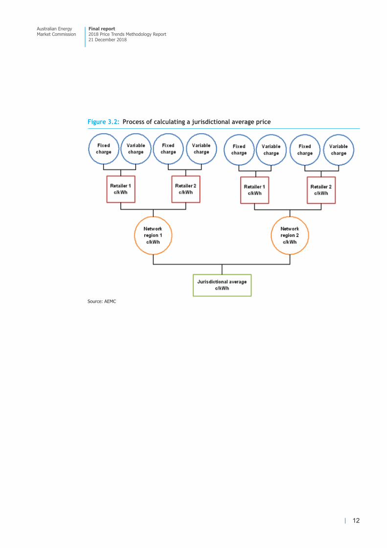
Figure 3.2: Process of calculating a jurisdictional average price 0

Source: AEMC

12



4 OVERVIEW OF NETWORK REGULATION AND COST ESTIMATION The network component of a consumer bill covers the costs associated with consumers using the transmission and distribution networks. Transmission costs relate to the transportation of electricity from generating sites to substations. Distribution costs are those related to transporting electricity from substations to consumer premises. Network charges also include the cost of metering services for most consumers.

This chapter outlines:

why networks are regulated •

who regulates networks •

how networks are regulated •

how this analysis estimates network costs as a component of the bill.18 •

4.1 Why networks are regulated Electricity networks are natural monopolies, in that they require large long term investments and achieve declining average costs with increased output. This means it is more efficient for network services to be supplied in an area by a single provider than for multiple networks to provide services.

As there is no competition for network services, network service providers (NSPs) are economically regulated to encourage efficient investment in and operation of the electricity network.

4.2 Who regulates networks Networks are regulated by the Australian Energy Regulator (AER) in the NEM and Northern Territory, and by the Economic Regulation Authority (ERA) in Western Australia.

It is the role of the AER and ERA to set the maximum revenues that a NSP can charge for the services they provide. Regulatory revenues are usually set every five years, as this regulatory control period is considered reasonable to provide a stable investment environment.

In addition to the regulatory authorities and the NSPs, the Federal Court of Australia may also have a role in determining network costs. The Federal Court may undertake judicial review of any AER decisions if NSPs challenge the regulatory decisions.19 The grounds for review must relate to the legality of the administrative decisions (e.g. an error in law), not the merits of the decision. This follows the 2017 decision by the Commonwealth government that abolished the ability of NSPs to appeal decisions to the Australian Competition Tribunal for

18 Further information on how networks are regulated is available in the AEMC’s “Electricity network economic regulatory framework review 2018”, available at https://www.aemc.gov.au/markets-reviews-advice/electricity-network-economic-regulatory-framew-1

19 The AER’s determinations are subject to judicial review under the Administrative Decisions (Judicial Review) Act 1977 (Cth).

13



limited merits review. As such, the only appeal available to NSPs is now on judicial grounds through the Federal Court of Australia.

4.3 How networks are regulated Incentive regulation

Network service providers are regulated under an incentives framework, which contains regulatory standards relating to the safety, reliability and security of electricity supply and obligations to enable connection to the electricity network.20

The regulatory model provides the NSPs with an incentive to operate efficiently. At the beginning of the regulatory control period, the regulator determines the revenue that can be earned over the period. This revenue is based on the regulator’s assessment of the costs the NSP will incur in providing network services, and includes a return on its capital. If the NSP can operate more efficiently than forecast (i.e. at lower cost) then it can retain the difference between the regulator’s forecast and its actual costs in the immediate regulatory period.21

From a consumer perspective, this model also has benefit. The regulator uses the revealed performance of NSPs in one regulatory period to determine the revenue cap for the next period. Therefore, if a business achieved efficiency gains in a regulatory control period, and benefits through higher earnings, consumers will benefit in the next period through lower regulated revenues and lower consumer prices. This is shown in Figure 4.1 below.

20 It is noted that large-scale generators pay for direct connection costs to the transmission network.21 This is given effect through the efficiency benefit sharing scheme in relation to opex, and the capital expenditure incentive

guideline in relation to capex.

Figure 4.1: Determining network revenue 0

Source: AEMC

14



A building block model informs revenue determinations in the NEM

The AER uses a number of components, known as building blocks, to calculate the allowed revenue for NSPs in each regulatory period:

capital costs, which consists of capital expenditure (capex), the regulatory asset base •(RAB), the weighted average cost of capital (return on capital) and depreciation operating expenditure (opex) •

other components, including tax and innovation allowances, efficiency carry-overs from •capex and opex, and incentive schemes including the Service Target Performance Incentives Scheme (STPIS) and Demand Management Incentive Scheme (DMIS).

The components are shown in Figure 4.2 below.

In considering the above costs, the AER uses a combination of benchmarking, forecasting and networks’ revealed costs in determining the reasonable costs on which to base its revenue determination.

Importantly, the AER does not approve each specific NSP project or program. Rather, once the different building blocks are added up to provide a total revenue amount, it is for the NSP to decide how to spend that amount to meet its regulatory requirements. This provides NSPs with the discretion to provide services using any combination of:

network or non-network options •

opex and capex based approaches •

technologies •

inputs from third parties or direct investment in assets. •

Network service provider tariffs in the NEM

Figure 4.2: Components of the building block model 0

15



After the regulator determines the total revenue for each NSP, NSPs develop tariffs to recover the allowed revenue. Transmission network service providers (TNSPs) pass their costs through to distribution network service providers (DNSPs). DNSPs charge retailers for their customers’ use of the network, and retailers then decide on the structure of pricing they use in retail electricity prices.

The regulator also decides how the allowed revenue can be translated into actual charges to retailers. There are typically two approaches:

a revenue cap - which sets the allowed revenue a NSP can recover. •

a weighted average price cap - which sets the average price level that a NSP can charge. •

Under a revenue cap, the total revenue is locked in over the regulatory period. NSPs can change their prices as long as they meet the cap.

Under a weighted average price cap, the revenue is not fixed. Instead it changes with changes in demand. If demand is above forecast, then higher revenue will result. Conversely, lower demand will result in lower revenue. In this way, networks subject to the weighted average price cap bear demand risk that revenue capped network businesses avoid.

Currently all of the DNSPs other than EvoEnergy (formerly ActewAGL) are regulated under revenue caps. The NER also prescribes that a revenue cap approach must be used for all TNSPs. Prior to this, they were subject to a weighted average price cap or hybrid models.

DNSP prices are also required, under the NER, to reflect the efficient costs of providing network services to each customer. To achieve this, DNSPs must comply with four pricing principles:

each network tariff must be based on the long run marginal cost of providing the service •

the revenue to be recovered from each network tariff must recover the network business’ •total efficient costs of providing services in a way that minimises distortions to price signals that encourage the efficient use of the network by consumers tariffs are to be developed considering the impact on consumers of changes in network •prices and develop pricing structures that are able to be understood by consumers network tariffs must comply with any jurisdictional pricing obligations imposed by state or •territory governments.22

DNSPs produce an Annual Pricing Proposal before each new financial year (or calendar year for Victorian network businesses) for approval by the AER. These proposals set out the prices for each different tariff class23 for the following year. In these proposals, the overall network use of service (NUOS) charge for each tariff class is broken down into the:

transmission use of service charge (TUOS) •

distribution use of service charge (DUOS) •

22 If network businesses need to depart from the above principles to meet jurisdictional pricing obligations, they must do so transparently and only to the minimum extent necessary.

23 A tariff class is a set of charges (such as fixed supply charge, usage charge/s) which applies to a particular group of customers. These groupings are typically defined by the customers annual usage level, voltage level required, or whether they are residential, small business or large business consumers.

16



metering charge (capital and non-capital) •

jurisdictional scheme costs (if applicable). •

Retailers use the approved Annual Pricing Proposal from each DNSP to inform their standing and market offers to consumers.

Western Australian network tariffs

In the South West Interconnected System (SWIS), Western Power’s electricity network is regulated by the ERA. The regulation of Western Power includes:

Access arrangements - the ERA determines the total revenue for the five year •regulatory period. The access arrangement covers prices, services, policies and terms and conditions for access to the Western Power network. Western Power’s proposal also details its five year investment plan for the period, which will ensure customers can continue to enjoy a good quality of service while network safety, security and capacity is improved. In doing this the ERA ensure Western Power:

complies with the requirements of the Access Code •meets the Access Code objective of promoting economically efficient investment in, •and operation and use of, electricity networks and services of networks in Western Australia, in order to promote competition in electricity retail and wholesale markets24 meets the service standards of each on its reference services. The ERA monitors and, •at least once a year, must publish Western Power’s actual service standard performance against its benchmarks.

Annual price lists for network charges - Western Power’s access arrangement •requires it to submit to the ERA a proposed price list and supporting information for the next pricing year. The ERA assesses the proposed price list to ensure it complies with the price control and pricing methods in Western Power’s access arrangement.

4.4 How this analysis estimates network costs This analysis relies on actual network costs when they are available, and projected costs in other years.

Given different Network Service Providers (NSP) have different regulatory control periods, the mix between actual and projected network costs differs by jurisidiction. Network businesses typically publish their prices shortly before they come into effect. Published prices are typically available for the first two years of the analysis period.

In this report actual DNSP tariffs are used for 2017-18 and 2018-19. For 2019-20 and 2020-21:

where final decisions have been made, the tariffs from the previous year are escalated by •the difference between the allowed (smoothed) revenue from the previous year to the next year.

24 Economic Regulation Authority, Electricity Network Access Code 2004 - Guidelines for Access Arrangement information, 6 December 2010, p1.

17



where a decision has not been finalised, the previous year’s tariff is held constant in •nominal terms.

The specific regulatory decisions by jurisdiction are described in chapter 3, but are summarised in Figure 4.3 below which shows the basis on which each jurisdiction’s network tariffs have been determined.

The detailed tariff information used to estimate network cost components is provided in Appendix A. This table includes the tariff classes used from each DNSP’s pricing proposal with the corresponding (actual) charges and growth rates for the transmission, distribution and metering charges.

4.5 Metering costs Competition in metering began in all jurisdictions other than Victoria, Western Australia and the Northern Territory on 1 December 2017. This change means metering and related services are now provided under a competitive framework,25 whereas previously metering costs were all regulated.26 Over time this change will affect how consumers pay for their metering services and therefore how they are accounted for in these annual reports.

Historically metering has been a regulated service provided by a DNSP, with Type 6 accumulation meters being the standard meter for residential installations. Even though

25 As established by the AEMC through the Expanding competition in meterings and related services rule change. For more information please see: https://www.aemc.gov.au/rule-changes/expanding-competition-in-metering-and-related-serv.

26 The AER changed the classification of the metering services in the NEM jurisdictions (other than Victoria) through the most recent set of DNSP determinations. For more information see the discussion papers Classification of metering services for each jurisidiction and final determinations for each DNSP.

Figure 4.3: Summary of approaches for estimating network costs 0

Note: Network costs are set on a financial year in all jurisdictions except Victoria, where network costs are set on a calendar year. ^In Tasmania, Western Australia (SWIS) and the Northern Territory, both transmission and distribution network services are provided by the same business. *In NSW and the ACT, the latest available AER remittal decision or business’ proposed remittal, that was available up until 8 November 2018, has been incorporated into the estimate of network costs. *ACS metering costs are determined from the respective distribution network service provider’s annual pricing proposal or the AER’s draft or final determination.

18



competition in metering came into effect on 1 December 2017, metering services will still be provided by DNSPs for the Type 6 accumulation meters as an Alternative Control Service27 until a consumer’s meter is replaced with a ‘smart’ meter.28Replacement can occur for a range of reasons, including breakage or because a consumer installs solar panels on their premises. New and replacement meters will be Type 4 smart meters, and these will be competitively supplied by retailers or metering coordinators.

The costs described in this report are for a representative consumer in each jurisdiction. Even though the process of transitioning to competitively supplied metering services has commenced in all NEM jurisdictions other than Victoria, the representative consumer (in all NEM regions other than Victoria) still has a Type 6 accumulation meter owned by a DNSP. For this reason metering charges will still be part of the network costs in this year’s report.

Importantly, metering costs have been separately identified as a specific component of the network costs (along with transmission network costs and distribution network costs). In future years, if the representative consumer has a smart meter rather than an accumulation meter, then metering costs will be reflected in the retail or residual component of the cost stack rather than in the network component.

27 An Alternate Control Service is a type of service provided by a DNSP and is regulated by the AER. The service is provided on a cost basis and is only paid for by the consumers when they use it.

28 If a customer’s meter is working properly and a competitive supplier wants to replace it with a smart meter, the customer can opt out of the smart meter installation.

19



5 WHOLESALE ELECTRICITY COSTS The wholesale electricity cost estimates that are used in this analysis are based on modelling undertaken by EY. EY’s modelling approach is explained in detail in its wholesale modelling report,29which is available on the 2018 Residential Electricity Price Trends project page on the AEMC website.30

This section describes the key concepts and summarises the calculation methods used by EY in estimating wholesale costs. This includes:

wholesale costs for the NEM, including an explanation of: •

modelling of wholesale electricity purchase costs •market fees, ancillary service costs and network losses •

wholesale costs for Western Australia, including an explanation of: •

long-run marginal cost •market fees and ancillary service costs •

wholesale costs for the Northern Territory. •

5.1 Wholesale costs in the NEM Wholesale costs in the NEM are based on estimates of wholesale electricity purchase costs, market fees, ancillary services and network losses.

5.1.1 Wholesale electricity purchase costs

Wholesale electricity purchase costs were estimated for each jurisdiction in the NEM from 2017-18 to 2020-21 using a blended method:

where possible, the analysis uses observable futures contract prices that retailers use to •build up their hedge contract book over time where limited forward contract data were available, then a forecast of spot market •outcomes and a contract premium was used.

Figure 5.1 and Figure 5.2 below provides a simplified overview of the approach for estimating wholesale electricity purchase costs, which involves:

market modelling of wholesale spot prices - used to determine the risk for a retailer •associated with uncertain wholesale costs, so that decisions around hedging can be made to manage this risk. This informs retailer’s decisions regarding the portion of their load that it makes economic sense to enter into futures contracts, and the remaining portion of their load that is better left exposed (unhedged) to the wholesale spot market. determining contract prices using observed ASX futures contract prices (where available) •and modelled wholesale prices which include an implicit hedge premium

29 EY, Residential Electricity Price Trends - Wholesale Market Costs Modelling 2018, 8 November 2018.30 See: aemc.gov.au and the 2018 Residential Electricity Price Trends project page.

20



exponential hedging to reflect the way in which small and large retailers progressively •build up their hedge books over a period of 12 and 24 months respectively, prior to the delivery period weighting hedge outcomes by the market share of small and large retailers in each •jurisdiction.

Figure 5.1: Process for estimating wholesale electricity purchase costs for 2017-18 and 2018-19*

0

Source: *For Victoria this method was applied to the 2018 and 2019 calendar years. Note: A separate outcome is calculated for one year hedging and two-year hedging. These outcomes are then weighted by the market

share of large and small retailers in the region. The result of that weighting is the estimated annual wholesale purchase cost for the jurisdiction.

21



The methodology for estimating wholesale costs is explained in more detail below.

Market modelling of wholesale spot prices

Wholesale spot prices are modelled to determine the risk for a retailer associated with uncertain wholesale costs, so that decisions around hedging can be made to manage this risk. This informs retailer’s decisions regarding the portion of their load that it makes economic sense to enter into futures contracts, and the remaining portion of their load that is better left exposed (unhedged) to the wholesale spot market.

EY’s market modelling of wholesale spot prices is an estimate of the lowest cost generation mix capable of meeting consumer demand in all 30 minute trading intervals of the reporting period, from 2017-18 to 2020-21. It is also required to meet a net revenue test, so that the revenue a generator receives from generating is equal to its fuel costs, operations and maintenance costs, and annualised capital cost repayments. This method is used to determine the commercial viability of generators to operate in the market.

Figure 5.2: Process for estimating wholesale electricity purchase costs for 2019-20 and 2020-21*

0

Source: *For Victoria this method was applied to the 2020 and 2021 calendar years. Note: Synthetic hedging only uses modelled wholesale spot prices. The results of synthetic hedging and exponential hedging are

blended separately for the small retailer (12 month) and large retailer (24 month) hedging approaches.

22



The market modelling is based on a range of assumptions and historical information, including:

fuel prices •

constraint equations •

generator entry and exit •

generator outages •

bidding behaviour of market participants •

demand side participation •

solar PV, storage and electric vehicle uptake •

historical hourly and locational information on: •

wind and solar conditions to inform its expectation of generation from renewable •resources consumer demand •

This modelling was carried out for the following scenarios:

base case •

low demand •

high demand •

low fuel price •

high fuel prices. •

These modelled wholesale spot prices and regional demand forecasts provide an estimate of the fair value of hedging instruments, to manage the risk of uncertainty over a retailers’ wholesale costs. Synthetic hedging uses simulated hedging instruments and the Net System Load Profile (NSLP) in each region to determine the wholesale purchase cost each retailer is expected to face, while managing their risk in the wholesale spot market. The price of each hedging instrument is stationary in a sense that it is set and determined at the time when the simulation is being run.

The modelling determines the fair value of the three most commonly used hedging instruments (baseload swaps, peak swaps and $300 caps) and the efficient combination of these hedging instruments, to be purchased over time by a retailer to manage their risk.

Retailer hedging costs for NEM jurisdictions will depend on the specific risk management strategy adopted by each retailer. This depends on the retailer’s expectations of future price volatility and its appetite for risk. Hedging enables retailers to reduce uncertainty over their wholesale costs, and the opportunity to offer stable pricing to consumers in the market.

Retailers purchase hedge contracts exponentially over time, prior to the delivery

period

There has been a significant change in the methodology used to calculate wholesale costs in this year’s report. Previous Residential Electricity Price Trends reports estimated retailers’ wholesale costs by forecasting spot market outcomes and applying a contract premium for

23



managing risk. This approach assumed that a retailer buys all its electricity and hedging contracts at a single point in time, so that its entire position is effectively purchased at the prevailing market price. However, it became apparent in the past two years, that with high volatility in forward prices after generator retirements, short term estimates made through a modelled approach were inconsistent with what was observed in the market.

For this reason, and to better reflect how retailers actually manage their wholesale costs, this report assumes retailers build up a hedge contract book over time.31 This determines the period of time over which they construct their hedging positions, and the levels of flexibility they have in the quantities of hedging they acquire over time.32

Larger retailers are assumed to have larger and more distributed customer bases, which •gives them more stable customer types and load profiles. This allows them to build their hedge contract book over a longer period. For these retailers a two-year book build was assumed. Smaller retailers are assumed to have a smaller customer base with a less certain load •profile. These retailers typically build up their hedge book over a shorter period. For these retailers a one-year book build was assumed.

It is assumed that for large and small retailers both progressively build up their hedge books over time, in an exponential manner. This means that greater volumes of hedging are purchased closer to the dispatch periods they cover. An indicative exponential hedge book build shape is shown in the figure below, referenced against the actual price of ASX baseload contracts. Figure 5.3 shows the volume of contracts that would be purchased over the period.

31 The modelling allowed the retailer to recover at least their wholesale costs in 48 out of 50 monte carlo price outcomes.32 In discusion with AEMC staff, a number of retailers commented that they operate within clear risk management frameworks.

24



It is also assumed that retailers complete their hedge book build around two months ahead of the contract delivery period. In most NEM jurisdictions that means retailers have achieved their desired level of contracting by the end of April each year, ahead of changing their prices at the beginning of July. In Victoria, retailers are assumed to have completed their contracting by the end of October, ahead of their price changes at the start of January.33 The two-month period after the contract book build is complete is then used by retailers to finalise their pricing, brief their customer contact teams, and to produce contractual and promotional material related to the price changes.

Figure 5.4 below shows how contracting informs retail pricing and smooths retailers’ costs by protecting them from the volatility of wholesale spot prices.

33 Retailers in the NEM generally change their prices after regulatory determinations are made by the AER.

Figure 5.3: Illustrative exponential build of retailer’s hedge contract book 0

Source: AEMC

25



The chart shows actual baseload contracts data for New South Wales, and how a retailer that builds their contracting book over time can achieve a stable average wholesale cost even when the forward contracting prices may fluctuate significantly over time. The length of time over which the contracting occurs has an effect on the wholesale cost that a retailer achieves for the hedged portion of their total load (customer demand).

The importance of building up a contracting position over time has been demonstrated in the past few years following the closures of the Northern and Hazelwood generators.34 Both these events lead to considerable volatility in wholesale spot and contracts markets. Retailers who had built up their contracting positions over longer periods were less exposed to the wholesale price increases, and therefore faced less pressure to pass on higher costs to consumers than retailers with shorter contracting positions. Conversely, retailers with shorter contracting positions are better placed to reduce prices when wholesale spot and contracting prices decrease.

Blended method using available observed futures contract prices and modelled

contract prices

Figure 5.5 shows the blended approach to estimating wholesale costs, which is based on:

34 The Hazelwood generator ceased operation in March 2017. A retailer determining prices for 2018-19 is assumed to have finalised its hedging position by April 2018. If it used a two year period to build its hedge book, the Hazelwood closure would have been approximately half way through that process.

Figure 5.4: How wholesale contracting smooths volatility and informs electricity retail prices 0

Source: AEMC

26



observed futures contract prices for the period of time for which they are available, and •

where futures contract prices are unavailable towards the end of the reporting period, •modelled wholesale prices that include an implicit hedge premium are used35

5.1.2 Market fees, ancillary services and network losses

Market fees and ancillary service costs were estimated by EY for this analysis.

Market fees are charges to market participants to cover the operational expenditures of AEMO. For the NEM EY has used AEMO’s estimated market fees for the years they were available and escalated the value in the forward years where necessary.36

Ancillary services are those services used by the market operator to manage key technical characteristics of the power system, such as frequency control. Actual costs were used in 2017 and 2018 for each region, and then extrapolated to future years with a linear trend.

Estimated transmission and distribution loss factors for residential customers were applied to wholesale electricity costs. The factors used were provided by EY, except for Tasmania where the factors were obtained from the Tasmania Energy Regulator’s (TER) retail pricing determination.

35 The weighted proportion of monte carlo modelled spot price outcomes from Probability of Exceedance (POE10) and POE50 demand traces, implicitly captures a contract premium.

36 Costs associated with the Reliability and Emergency Reserve Trader (RERT) were not included in the estimate of wholesale costs in this report. AEMO dispatched the RERT for the first time in the history of the NEM in 2017-18 in Victoria and South Australia.

Figure 5.5: Blended approach using available futures contract prices and modelled prices 0

Source: AEMC Note: If a retailer was using a 12 month hedging strategy, 6 months of contracting data is available for 2019-20 and no data for 2020-

21

27



5.2 Wholesale costs in Western Australia In the WEM, wholesale costs and the costs presented in this report were estimated based on a long-run marginal cost (LRMC).37

Long-run marginal cost (LRMC) approach

The LRMC of generation approach reflects the costs that a retailer would face if it were to build and operate a theoretical least-cost generation system to service its retail business.38 This approach is strongly influenced by key input assumptions relating to capex, opex and fuel costs.

The approach makes available the following technologies to meet demand:

combined cycle gas turbines •

open cycle gas turbines •

black coal •

wind •

single axis tracking solar •

utility scale storage.39 •

In addition to meeting the representative customer load, additional capacity was included to act as a system reserve. To maintain consistency with the 2017 Residential Price Trends Report a 15% reserve margin has been applied.

Market fees, ancillary service costs

In the WEM, market fees include the costs of AEMO as well as the costs associated with System Management and the Economic Regulation Authority. Those fees were estimated in a similar way to the NEM. Actual costs were used in 2017 and 2018 and then extrapolated to future years with a linear trend.

For more information on the methodology for estimating wholesale costs in the WEM, refer to EY’s report.40

5.3 Wholesale costs in the Northern Territory Wholesale electricity costs for 2017-18 to 2020-21 were provided to the AEMC by the Northern Territory Government for the Darwin-Katherine network. This included transmission and distribution loss factors for residential customers.

37 An alternative estimate of wholesale costs in the WEM was also developed by EY and is outlined in their report on the AEMC’s website. The alternative method, based on market modelling, was developed as a comparison to provide insights for the Western Australian government.

38 The stand-alone LRMC approach is discussed in more detail in EY’s report “Residential Electricity Price Trends - Wholesale Market Costs Modelling 2018”.

39 Only OCGT, wind and black coal was built in EY’s modelling to meet demand.40 EY, Residential Electricity Price Trends - Wholesale Market Costs Modelling 2018, Australian Energy Market Commission, 8

November 2018.

28



6 THE LRET AND WHOLESALE ELECTRICITY COSTS This report examines wholesale costs and environmental costs separately, and focusses strongly on the direct costs of each component. However wholesale market outcomes are increasingly interconnected with environmental policies.

Under the Large scale renewable energy target (LRET), retailers are obliged to acquire large-scale generation certificates (LGCs) created by renewable generators. The costs of LGCs are passed through to both small and large consumers. The direct costs of these environmental policies are described in detail in Chapter 7 of this report. However the LRET also has additional indirect effects on wholesale electricity costs.

6.1 The LRET and wholesale electricity costs The LRET scheme design incentives new investment in renewable generation such as solar PV and wind. To date this has largely been wind generation, although increasing amounts of solar generation are also being developed.

Figure 6.1 shows the effect the LRET has on wholesale electricity price dynamics in the short and medium term.

In the short-term, as wind and solar generators have lower operating costs compared with gas- and coal-fired generators, they are likely to submit lower offer prices and be dispatched by AEMO early in the merit order. This can put downward pressure on wholesale electricity costs, as Figure 3.2 shows the supply curve shifts down. The resulting excess supply, leads to wholesale price decreases, shown in the diagram by a decrease in price from Price¹ to Price².

Figure 6.1: Effect of the LRET on short and medium term electricity prices 0

Source: AEMC

29



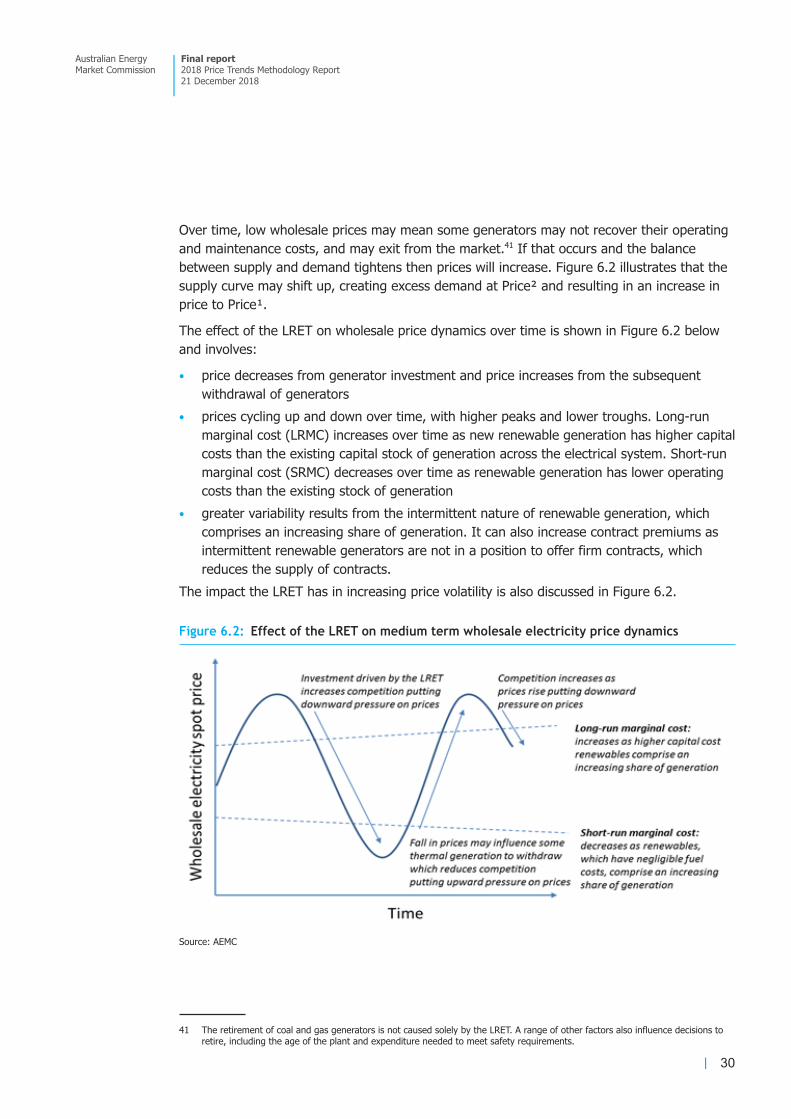
Over time, low wholesale prices may mean some generators may not recover their operating and maintenance costs, and may exit from the market.41 If that occurs and the balance between supply and demand tightens then prices will increase. Figure 6.2 illustrates that the supply curve may shift up, creating excess demand at Price² and resulting in an increase in price to Price¹.

The effect of the LRET on wholesale price dynamics over time is shown in Figure 6.2 below and involves:

price decreases from generator investment and price increases from the subsequent •withdrawal of generators prices cycling up and down over time, with higher peaks and lower troughs. Long-run •marginal cost (LRMC) increases over time as new renewable generation has higher capital costs than the existing capital stock of generation across the electrical system. Short-run marginal cost (SRMC) decreases over time as renewable generation has lower operating costs than the existing stock of generation greater variability results from the intermittent nature of renewable generation, which •comprises an increasing share of generation. It can also increase contract premiums as intermittent renewable generators are not in a position to offer firm contracts, which reduces the supply of contracts.

The impact the LRET has in increasing price volatility is also discussed in Figure 6.2.

41 The retirement of coal and gas generators is not caused solely by the LRET. A range of other factors also influence decisions to retire, including the age of the plant and expenditure needed to meet safety requirements.

Figure 6.2: Effect of the LRET on medium term wholesale electricity price dynamics 0

Source: AEMC

30



6.2 The LRET and price volatility Uncertainty is normal and inevitable in the wholesale electricity market. Innate risks in the power system, such as transmission or power station outages and unforeseen changes in demand, are reflected in movements in spot prices. Being exposed to sudden and volatile price movements is therefore an inherent aspect of participating in the wholesale spot market.

The increasing intermittency of generation can lead to more volatile wholesale electricity spot prices. Price volatility in the wholesale electricity spot market can occur as the market responds to unexpectedly high or low demand or supply. Weather related events and generator or interconnector outages can contribute to volatility. For example, high wholesale price events have in the past corresponded to times when wind generation or rooftop solar PV production is low and there is an outage in a generator or interconnectors are constrained.

The level of volatility is also affected by the extent of contracts in the market. This is discussed in section 6.3 below.

6.3 The LRET and the wholesale electricity contract market Increased volatility in spot prices increases the overall level of risk retailers must manage. Retailers can manage the risk of volatile electricity spot prices by purchasing contracts (such as swaps, caps and options) and by owning generators (i.e. vertical integration).

More contracting in a market lowers risk for both retailers and generators. This can lead to lower wholesale spot market prices. Generators enter into contracts to recover their costs and a rate of return. Therefore, they no longer need to recover all of these costs from the electricity spot market. Contracted generators, when generating to contracted levels, are to some extent indifferent to spot prices and therefore bid to achieve output that matches contracted volumes. The effect of higher volatility on retail prices is also reduced with higher levels of contracting as retailers are less exposed to spot prices. More contracting can therefore lead to lower risk exposure, a less volatile market and lower wholesale price levels. Figure 6.3 shows the indicative reduction in risk and volatility from contracting over a given level of capacity.

31



Where there is greater price volatility in the spot market, the costs of contracts may increase. Higher contract prices provide an incentive for increased investment in generating assets. When built, this should lead to electricity prices stabilising as there is increased supply to meet demand.

The LRET provides incentives for increased quantities of renewable generation to enter the market, even when demand is flat or falling. This is because the revenue that these intermittent generators receive from the scheme is additional to that available from the wholesale market and the LGC penalty price is higher than the expected long-run cost of investing in new intermittent generation.

The technical characteristics of intermittent generation are also not suited to offering the type of hedging contracts that thermal generators can offer. In particular, intermittent generators without firming capabilities do not add to the supply of traditional swaps and caps. This affects the level of liquidity in contract markets and may undermine the ability of retailers to hedge their customer loads against the risk of volatile spot market prices.

The economic characteristics of intermittent generators are also different from thermal generators. Their initial capital costs are relatively high, although these continue to fall rapidly, and their marginal costs of operating are negligible. These economic characteristics let these generators displace thermal generators (which have higher marginal or operating costs, primarily due to fuel costs) at times when they are generating. Over time, to the extent to which the LRET contributes to the exit of thermal generation but does not incentivise investment in firming technologies, it may result in a tighter supply-demand balance and lead to higher wholesale prices.42 As the LRET target for 2020 is expected to be met through the large volume of new renewable investments in the coming years, and the

42 The South Australian forward contract market is one where this is situation has been observed.

Figure 6.3: Effect of hedge contracting on spot market volatility 0

Source: AEMC

32



price of large-scale generation certificates (LGC’s) is expected to fall significantly as a result, the LRET is not expected to drive additional investment in new renewable projects after 2020.

The overall impact of the LRET has therefore been to drive down wholesale prices in the short-term but, in the absence of policies and incentives to encourage investment in replacement generation and firming technologies, it contributes to periods of more volatile and potential higher wholesale prices.

In addition, given that fewer generators may provide contracts, the risk faced by retailers from volatile spot prices may increase due to the inability to hedge their positions. Over the longer term, this may potentially affect the level of retail competition.

33



7 INTERCONNECTORS AND THEIR EFFECT ON WHOLESALE COSTS Transmission networks that transport electricity between regions are referred to as interconnectors. They affect the balance of supply and demand across regions, which influences wholesale electricity costs via both the spot market and contract market.

This section provides an overview of:

interconnectors in the NEM •

the effect interconnectors have on wholesale electricity prices and contract market •outcomes how interconnecters are funded •

the physical limits of interconnectors. •

7.1 Interconnectors in the NEM The interconnected transmission network in the NEM supports a reliable supply of electricity and the efficiency of the wholesale market by allowing electricity to be bought and sold across regions.

Interconnectors consist of transmission infrastructure located on each side of a regional boundary, connected by a set of high-voltage transmission lines. Figure 7.1 shows the location of existing interconnectors in the NEM.

34



In addition to the existing interconnectors, AEMO’s ISP sets out a larger potential role for interconnectors across the NEM by 2040. The report splits potential projects into three groups according to the indicative timing of completion.

Group 1 interconnector projects have an indicative timing of 2020, and include:

upgrades to the Queensland-New South Wales interconnectors adding 460MW/190MW •capacity at an estimated cost of $142 million43 upgrades to the Victorian-New South Wales interconnector resulting in additional capacity •of 170MW at a cost estimate of $80 million.

The Group 2 projects have indicative timing of 2020-2030, and include:

further upgrades to the Queensland-New South Wales interconnectors resulting in •additional capacity of 460MW/568MW at a cost estimate of $525 million further upgrades to the Victorian-New South Wales interconnector resulting in additional •capacity of 120MW at a cost estimate of $5 million build the Riverlink interconnector between South Australia and New South Wales, •resulting in additional capacity of 1,500MW at a cost estimate of $1.27 billion.

43 This refers to 460MW additional capacity from Queensland to NSW, and 190MW additional capacity from NSW to Queensland.

Figure 7.1: Interconnectors in the NEM 0

Source: AEMO Note: Maximum annual revenues for regulated interconnectors are set by the AER. A market interconnector (also known as a merchant

interconnector) obtains revenue by trading on the spot electricity market. For more information on interconnectors see Australian Energy Market Commission, Decision report: Last resort planning power – 2016 review, 13 October 2016.

35



The Group 3 projects have indicative timing of 2030-2040, and include:

increasing the transfer from Snowy 2.0 and other REZs to Victoria and New South Wales •by building the SnowyLink interconnector, resulting in additional capacity of 3,000MW at a cost estimate of $1.171 billion further development of the SnowyLink interconnector, resulting in additional capacity of •2,500MW at a cost estimate of $1.7 billion building a second Victorian-Tasmanian interconnector, resulting in additional capacity of •700-1,000MW at a cost estimate of $1.285 billion.

As none of the above projects are included in current AER network determinations, the costs are not part of this analysis. If they proceed and are operational before the end of 2020-21, then they may impact on network costs and consumer pricing and billing outcomes.

In terms of scale, the above projects have an estimated capital cost of approximately $6.2 billion, against a combined regulated transmission asset base of $20.5 billion in the NEM in 2017.

7.2 The effect of interconnectors on the market Wholesale electricity spot market effects

Interconnectors allows electricity in lower priced regions to flow to higher priced regions, which reduces the cost of meeting demand in the NEM and the degree of price separation between regions. It can also contribute to a reduction in price volatility within regions.

Interconnection can cause wholesale electricity prices to reduce in one region and increase in another. The effect of interconnectors on wholesale electricity spot prices is illustrated in Figure 7.2.

36



Inter-regional settlements residue

Price separation of regional spot prices often occurs when interconnector capacity is not sufficient to equalise the spot price flowing from a lower to a higher priced region.

Figure 7.2: Interconnectors in the NEM 0

Source: AEMC

37



The difference between the price paid in the importing region and the price received in the exporting region, multiplied by the amount of flow for each interconnector for a trading interval, results in surplus inter-regional settlements residue.

Since August 1999, AEMO and its predecessor, the National Electricity Market Management Company (NEMMCO) have been holding auctions where units, representing a right to a certain portion of that money could be purchased by auction participants. These units are called settlement residue distribution units.

Contract market effects

Interconnectors are a partial substitute for local generation in a region in that imported electricity can be a substitute for increasing generation within a region. However, hedge contracts cannot be written to the same extent against the capacity supplied by interconnectors, as they can for local generation due to interconnectors having inter-regional flow constraints. Settlement residue distribution units do provide some help in underwriting inter-regional hedge contracts, but they do not offer the same level of firmness as local hedge contracts. This affects the level of competition and therefore liquidity in the electricity contract market in each NEM region.44

In the case where there is increasing reliance on interconnection to meet demand, lower levels of generator competition may result in reduced contract market liquidity. Generators and retailers in the region are likely to have more exposure to the electricity spot price and fewer options to manage this risk at an efficient cost.

Where there is sufficient competition among generators to provide a liquid contract market, interconnection may have little effect on competition.

7.3 Infrastructure costs of interconnection Interconnectors can either be regulated or merchant.

Regulated interconnectors earn revenues determined by the AER, regardless of flows across the interconnector. These revenues are recovered from consumers through the network component of electricity bills. To be regulated, an interconnector must pass the Regulatory Investment Test for Transmission (RIT-T).45

Merchant interconnectors earn revenue by buying electricity in one region and selling it in another when there is a price difference between the two regions.46 Their revenues are not fixed by the AER. Anyone can build a merchant interconnector, including governments. They

44 On 10 October 2017 the AEMC made a rule that allows for, but does not mandate, the introduction of secondary trading of settlement residue distribution units via the same auction process already facilitated by AEMO. A more liquid secondary market of settlement residue distribution units is likely to offer better protection against price separation between regions and lead to more efficient interregional hedging outcomes. AEMC, Rule determination - National Electricity Amendment (Secondary trading of settlement residue distribution units) Rule 2017, 10 October 2017.

45 The RIT-T promotes efficient investment in interconnectors and protects consumers from paying for interconnectors that are inefficient. It weighs up the costs and benefits of the interconnector over a 20-40 year period, including considering the costs and benefits of different solutions, scenarios for economic growth, and changes in demand and technology

46 For more information on interconnectors, see Australian Energy Market Commission, Last Resort Planning Power – 2016 Review, decision report, 13 October 2016, pp13-14.

38



do not need to pass the RIT-T. Basslink is currently the only example of a merchant interconnector in the NEM.

7.4 Physical limits of interconnectors Each interconnector has certain capacity which is the upper limit of electricity that can be carried between regions. In practice, limits elsewhere in the network mean that the actual transfer of capacity is often set at lower levels. Actual capacity may therefore vary between seasons, between peak and off-peak periods and according to flow directions.

The ability of the network to carry electricity (the ‘transfer capability’) is affected by a range of factors.47 For example, congestion may be caused by outages or maintenance operations because generators or particular network elements are unavailable, or are being temporarily operated at reduced capacity. Congestion is a normal feature of power systems and occurs because the power system must be maintained within specific physical limits. Factors such as capacity limits, thermal limits and frequency limits must all be managed to maintain the system in a secure operating state.

Constraints in transmission infrastructure further removed from regional boundaries can also affect electricity flows across regional boundaries. To this extent this happens, as shown in Figure 7.2, wholesale prices will separate across regions.

47 See also Australian Energy Market Commission, Congestion Management Review, 16 June 2008, p50.

39



8 ENVIRONMENTAL COSTS This section examines the environmental schemes that have been introduced by the Commonwealth and jurisdictional governments to encourage investment in renewable generation and encourage energy efficiency. These schemes are collectively referred to as environmental policies throughout this report and in the 2018 Price Trends Report.

Environmental schemes differ by jurisdiction and by duration. The direct costs of these schemes are included in the analysis for their known duration. If a scheme is legislated to end during the reporting period, or it is unknown whether or not the schemes will continue, then the cost of that scheme has not been included in the analysis.

It should be noted that the environmental scheme costs only include the direct costs of these policies.

8.1 Renewable energy target The Renewable Energy Target (RET) is a Commonwealth scheme which supports new renewable energy generation and reductions in greenhouse gas emissions. It consists of two components:

the LRET, which has a target of 33,000 GWh of additional renewable generation by 2020 •compared to 1997 levels. The LRET encourages companies to invest in large scale renewable energy generation, such as solar systems, wind farms, hydro stations and biomass generators. the SRES, which does not have a specific target. The SRES encourages households and •small businesses to install small scale systems, such as solar panels, solar hot water heaters, small scale wind or hydro systems, and air source heat pumps.

Both schemes provide investment incentives until 2030.

The renewable technologies generate certificates for each megawatt hour of energy that they produce. Retailers then have an obligation to purchase and surrender large-scale certificates (LGCs) and small-scale technology certificates (STCs) to the Clean Energy Regulator, in order to meet their RET obligations. The number of certificates each retailer must surrender is determined by the quantity of electricity they sell to their customers as a proportion of all electricity consumption. The costs of purchasing and surrendering these certificates are passed on to consumers in retail prices.

The cost of the LRET and SRES schemes are described below. Further detail is provided in EY’s report.48

LRET costs

The cost of the LRET to each retailer is calculated as the number of LGCs required for that year multiplied by the LGC price. The number of required LGCs for each year is determined

48 See EY, Residential Electricity Price Trends - Wholesale Market Cost Modelling 2018, November 2018. The Clean Energy Regulator explains the RET on its website. See http://www.cleanenergyregulator.gov.au/RET/Scheme-participants-and-industry/the-renewable-power-percentage

40



by the relevant acquisitions (or electricity purchases), for each retailer, multiplied by that year’s renewable energy percentage (RPP) as set by the Minister.

LGC prices

EY has estimated the LGC certificate price as the fair value of the subsidy required for a new entrant renewable generator entering into a power purchase agreement (PPA) to recover its fixed and variable costs. The technology that provides the lowest subsidy is considered to be the marginal generator that sets the LGC price for a particular year. This method approximates a market mechanism for setting LGC certificate prices.

Alternatively, LGCs can be purchased on the contract market. However because most large scale renewable projects are financed with PPAs, the volume of traded certificates is low. As such, the pricing of those certificates is not indicative of the longer term financing considerations for most large scale renewable generation investors.

The price of traded certificates tends to be higher than those sourced via PPAs, and is closer to the tax-effective shortfall charge of approximately $90 per megawatt hour.49 For this reason, larger retailers with more PPAs are assumed to face lower LGC prices than smaller retailers who face higher risks of spot market exposure.

Modelling the forward price of LGCs is complicated by PPAs which bundle the energy component with LGCs in a single price. Over time, if there is any change in the energy price component, the residual certificate price will also be adjusted but in the opposite direction as the bundled PPA price is constant over the period.

Setting the renewable power percentage

The renewable power percentage is set by the Minister for Energy by the end of March each year. It is based on the quantity of renewable generation needed to meet each year’s annual target. This is to incentivise large-scale renewable generation to meet the target of 33,000 GWh by 2020.

The calculation of the RPP is the quantity of renewable electricity required to meet the annual target (accounting for any prior year carry-overs) divided by the total electricity acquisitions (equivalent to their total customer base’s consumption level, less any exemptions, such as for emissions intensive trade exposed industries).

The Minister sets the RPP on a calendar year basis. Because this report is in financial years, the RPP needs to be translated into a financial year form. While previous Price Trends reports have used a 50/50 per cent split to do this translation, this report uses a 75/25 per cent split. This is considered to be a more accurate representation of how retailers estimate these costs and pass them through into retail prices, and is shown in the Figure 8.1 below.

49 The penalty price is variously referred to as being $90 or $65. The penalty is actually $65, but because it is not a tax deductible expense, it is regularly grossed up to $90.

41



The costs of the LGC and LRET for each financial year of the analysis are shown in Table 8.1 below.

Figure 8.1: Rationale for converting calendar year to financial year 0

Source: AEMC

42



Table 8.1: RET costs by year and jurisdiction

Note: The RRP was set by the Minister on 31 March 2017 and 2018. LGC Mercari market prices are as of 8 August 2018.

LARGE RETAILER SMALL RETAILER

CALENDAR

YEAR

CALCULATED

RPP

FINANCIAL

YEAR

FINANCIAL YEAR

EQUIVALENT NT RPP

AVERAGE

MARKET COST

OF LGC

LRET WHOLE-

SALE COST

COMPONENT

($/MWH)

LGC MERCARI

MARKET

PRICE

LRET WHOLESALE

COST COMPONENT

($/MWH)

2021 19.24% 2020-21 19.33% $40.30 7.79 $19.25 3.722020 19.58% 2019-20 19.16% $39.01 7.47 $24.50 4.692019 17.90% 2018-19 17.44% $38.67 6.74 $70.75 12.342018 16.05%* 2017-18 15.60% $38.13 5.95 $79.00 12.322017 14.22%*

43



Small-scale Renewable Energy Scheme costs

The cost of the SRES to each retailer is calculated as the number of STCs required for that year multiplied by the STC price obtained by each retailer. The number of required STCs for each year is determined by the relevant acquisitions (or electricity purchases), for each retailer, multiplied by that year’s small-scale technology percentage (STP) as set by the Minister.

Small-scale Technology Certificate prices

STCs are traded in the wholesale market, so the price depends on the supply and demand for certificates at any point in time. There is a minimum size for a trading parcel of 5,000 certificates. There is also a clearing house price of $40, so most variation in the traded market price is below $40.

The difference in the market and clearing house prices is largely related to the timing of payment for the certificates that a system will produce. Retailers and other purchasers will offer to buy the certificates that a system will generate, up-front at a discount. The alternative for the system owner is to sell these through the clearing house, but that will result in between six and nine months delay in payment. No interest is paid by the clearing house for the time between certificate assignment and payment.

Setting the small-scale technology percentage

The small-scale technology percentage is set in the same way as the RPP. The Minister for Energy sets the STP by the end of March each year, and it is set to adjust demand for certificates to balance supply, rather than any amount to meet a target like done in the LRET scheme.

The calculation is the estimated number of STCs to be created for the year (accounting for any prior year carry-overs) divided by the total electricity acquisitions (equivalent to their total customer base’s consumption level,ess any exemptions, such as for emissions intensive trade exposed industries).

As for the RPP, the calendar year STP is translated into a financial year figure using a 75/25 per cent split, as shown in Figure 7.1 above.

The costs of the STC and SRES for each financial year of the analysis are shown in Table 8.2 below.

44



Table 8.2: Calculation of STP from calendar to financial year

Note: *The STP was set by the Minister on 31 March 2017 and 2018

LARGE RETAILER SMALL RETAILER

CALENDAR

YEAR

CALCULATED

STP

FINANCIAL

YEAR

FINANCIAL

YEAR EQUIVA-

LENT STP

AVERAGE

MARKET

COST OF

STC

SRES WHOLESALE

COST COMPONENT

($/MWH)

STC CLEAR-

ING HOUSE

COST

SRES WHOLESALE

COST COMPONENT

($/MWH)

2021 20.58% 2020-21 19.18% $35.00 6.71 $40.00 7.672020 18.71% 2019-20 19.37% $35.00 6.78 $40.00 7.752019 19.59% 2018-10 17.71% $35.00 6.20 $40.00 7.082018 17.08% 2017-18 9.53% $35.00 3.33 $40.00 3.812017 7.01%

45



Calculating jurisdictional RET costs

Calculation of the RET costs by jurisdiction builds on the preceding analysis. The large and small retailer costs for both the LRET and SRES schemes are multiplied by the market share of each category of retailer (i.e. large or small) in each jurisdiction. This produces a dollar per megawatt price for both LRET and SRES which is then multiplied by the representative consumers’ consumption level in each jurisdiction to provide the jurisdictional specific LRET and SRES cost. These costs are in Table 8.3 below.

46



Table 8.3: RET costs by year and jurisdiction

Note: *A different methodology is used for Tasmania because the regulated residential tariff specifically states the RET costs for consumers for each financial year.

JURISDICTION

FINANCIAL YEAR SEQ NSW ACT VIC SA TAS* WA

LRET cost

($/MWh)

2020-21 $6.31 $7.13 $7.78 $6.05 $6.76 $7.79 $7.792019-20 $6.46 $7.02 $7.47 $6.29 $6.77 $7.47 $7.472018-19 $8.78 $7.64 $6.76 $9.13 $8.16 $6.74 $6.742017-18 $8.26 $6.97 $5.96 $8.67 $7.56 $5.95 $5.95

SRES cost

($/MWh)

2020-21 $7.06 $6.87 $6.71 $7.12 $6.96 $6.71 $6.712019-20 $7.13 $6.93 $6.78 $7.19 $7.02 $6.78 $6.782018-19 $6.52 $6.34 $6.20 $6.58 $6.42 $6.20 $6.202017-18 $3.51 $3.41 $3.34 $3.54 $3.46 $3.33 $3.33

Large retailer 63.65% 83.89% 99.75% 57.32% 74.68% 100% 100%Small retailer 36.35% 16.11% 0.25% 42.68% 25.32%

47



A summary of the RET calculation methodology follows:

Table 8.4: Summary of RET calculation method

Source: https://www.auroraenergy.com.au/Aurora/media/pdf/Aurora-Energy-pricing-july-2017.pdf and https://www.auroraenergy.com.au/Aurora/media/pdf/Aurora-Energy-pricing-july-2018.pdf

8.2 Other environmental schemes Other jurisdictional specific environmental schemes are also funded by residential electricity consumers. These schemes include energy efficiency incentives and feed-in-tariffs (FiT) payments for generation from solar PV systems.

Energy efficiency schemes

Jurisdictional energy efficiency schemes are designed to assist consumers in reducing their energy consumption. There are a range of measures that can be taken to improve energy efficiency including, for example:

providing funding for the purchase of efficient appliances such as fridges and freezers. •

using energy intensive appliances during off-peak times (for consumers on time of use •tariffs). educating small customers and businesses about their energy usage patterns and •behaviour to better equip them to use their energy efficiently. changing lighting from incandescent and fluorescent lamps to low energy LEDs. •

These schemes are funded by retailers, who pass the costs on to consumers. The schemes differ by jurisdiction. The cost of these schemes to consumers is shown in Table 8.5 below.

YEAR RET COST ESTIMATE

2017-18 The proportion of LRET and SRES costs were derived from RET costs using •EY’s LRET and SRES modelled costs for the NEM. Total RET costs were taken from Aurora Energy’s standing offer •determinations for July 2017 for 2017-18 and July 2018 for 2018-19. The percentage contribution for both the SRES and LRET is applied to the •RET costs taken from the offer determination to provide the LRET and SRES estimate for Tasmania.

2018-19

2019-20 The LRET and SRES costs from the previous year are escalated using the •respective trends established by EY.2020-21

48



Table 8.5: Costs of energy efficiency schemes

Source: Data supplied by jurisdictions Note: *As retailers in Victoria typically update their retail prices on a calendar year basis, Victorian VEU costs are included on a calendar year basis, as far as practicable using available information. VEU costs for the

2018 calendar year are based on 2017-18 costs; VEU costs for the 2019 calendar year are the average of 2018-19 and 2019-20; VEU costs for the 2020 calendar year are the average of 2019-20 and 2020-21; and VEU costs for the 2021 calendar year are based on 2020-21. It is noted that no targets are set beyond 2020, so VEU costs in 2020-21 are estimated based on an indicative target.

STATEDISTRIBUTION

AREA

NETWORK

CHANGE

SOURCE OF

CHARGE2017-18 2018-19 2019-20 2020-21

NSW

Ausgrid, Essential Energy, Endeavour Energy

Energy Saving Scheme - retailer obligation

NSW government - Department of Planning and Environment

Usage charge: $0.00171/kWh




ACT EvoEnergyEnergy Efficiency Improvement Scheme (EEIS)

ACT government - Environment, Planning and Sustainable Development Directorate





SA SA Power NetworksRetailer Energy Efficiency Scheme (REES)

SA government - Department for Energy and Mining





VIC*

Jemena, AusNet Services, United Energy, CitiPower, Powercor

Victorian Energy Upgrades (VEU)

VIC government - Depart of Energy, Environment and Climate Change





49



Feed-in-tariff (FiT) schemes

Solar PV feed-in-tariffs are either net or gross tariffs for electricity generation. A gross FiT means that the consumer receives a payment for all electricity generated by the solar PV system, whereas under a net FiT the consumer is only paid for the electricity that is exported to the grid.50

The level of FiTs varies by jurisdiction. Previous schemes provided a financial incentive for residential consumers to install solar PV systems at a time when the capital cost of the systems was high and the payback periods were long. However, given significant reductions in the cost of solar systems, most FiT payments are now moving to being more representative of the value of the electricity supplied to the grid. Different jurisdictions have different approaches to valuing and calculating FiTs51, and the level of incentive provided will vary according to whether the jurisdiction has any broader environmental targets.

The cost of these schemes are spread across the whole customer base. Costs are identified by DNSPs in their network tariff proposals, and are then passed on to consumers in retail prices. The cost estimates used in this analysis were taken from each applicable DNSP’s Annual Pricing Proposal. The costs of the schemes are summarised in Table 8.6 below.

50 Details on the current and closed FiT tariff schemes can be found on the websites of jurisdictional governments and electricity retailers.

51 For example, Victorian FiTs include a value for offsetting greenhouse gas emissions. Other jurisdictions do not explicitly value this component.

50



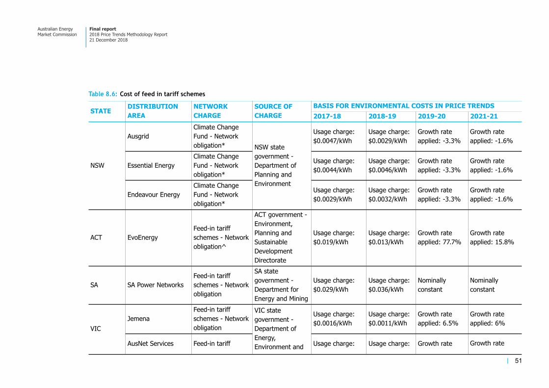
Table 8.6: Cost of feed in tariff schemes

STATEDISTRIBUTION

AREA

NETWORK

CHARGE

SOURCE OF

CHARGE

BASIS FOR ENVIRONMENTAL COSTS IN PRICE TRENDS

2017-18 2018-19 2019-20 2021-21

NSW

AusgridClimate Change Fund - Network obligation* NSW state

government - Department of Planning and Environment



Growth rate applied: -3.3%


Essential EnergyClimate Change Fund - Network obligation*





Endeavour EnergyClimate Change Fund - Network obligation*





ACT EvoEnergyFeed-in tariff schemes - Network obligation^

ACT government - Environment, Planning and Sustainable Development Directorate



Growth rate applied: 77.7%


SA SA Power NetworksFeed-in tariff schemes - Network obligation

SA state government - Department for Energy and Mining



Nominally constant

Nominally constant

VICJemena

Feed-in tariff schemes - Network obligation

VIC state government - Department of Energy, Environment and




Growth rate applied: 6%

AusNet Services Feed-in tariff Usage charge: Usage charge: Growth rate Growth rate

51



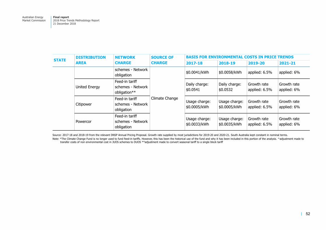
Source: 2017-18 and 2018-19 from the relevant DNSP Annual Pricing Proposal. Growth rate supplied by most jurisdictions for 2019-20 and 2020-21. South Australia kept constant in nominal terms. Note: *The Climate Change Fund is no longer used to fund feed-in tariffs. However, this has been the historical use of the fund and why it has been included in this portion of the analysis. ^adjustment made to

transfer costs of non environmental cost in JUOS schemes to DUOS **adjustment made to convert seasonal tariff to a single block tariff

STATEDISTRIBUTION

AREA

NETWORK

CHARGE

SOURCE OF

CHARGE

BASIS FOR ENVIRONMENTAL COSTS IN PRICE TRENDS

2017-18 2018-19 2019-20 2021-21

schemes - Network obligation

Climate Change

$0.0041/kWh $0.0058/kWh applied: 6.5% applied: 6%

United EnergyFeed-in tariff schemes - Network obligation**

Daily charge: $0.0541




CitipowerFeed-in tariff schemes - Network obligation





PowercorFeed-in tariff schemes - Network obligation





52



9 RESIDUAL COMPONENT OR RETAIL COST The last part of the electricity cost stack is the residual component or retail cost. Either the residual component or retail cost is used depending on the jurisdiction.

9.1 Residual component As retailer operating costs and margins are not usually observable, the analysis in this chapter estimates the residual as the difference between billing outcomes (based on retail prices multiplied by consumer consumption) and the other components of the cost stack. This is a top-down methodology, starting with a known billing outcome, removing known costs, and deriving the unknown (residual) component. This is shown in Figure 9.1 below.

The residual component was derived for 2017-18 and 2018-19 (2018 for Victoria) by subtracting the wholesale, network and environmental cost components from the residential bill. This residual component was then escalated by an assumed inflation rate of 2.5 per cent for future years in the reporting period. Exceptions to this are:

in Western Australia the cost stack includes a retail cost component52 •

in the Northern Territory there is a cost differential.53 •

In aggregate, the residual component consists of the retailer’s operating costs (opex), customer acquisition and retention costs (CARC), return on investment (ROI), and any errors in estimating the other supply chain cost components, as shown in the Figure 9.2 below.54

52 The retail component is provided by the Western Australian Public Utilities Office for Synergy’s efficient retailer operating costs and retail margin.

53 The cost differential refers to the difference between the residential price set by the Northern Territory Government and the cost of supply (which includes the cost of wholesale, networks and environmental policies). This is to reflect the effective subsidy provided to consumers in the Northern Territory as the cost of supply is higher than the residential price set by the government, and paid by consumers.

54 For a detailed explanation of the elements that comprise the retail margin, please refer to the AEMC’s Retail Competition Review 2017.

Figure 9.1: Method of deriving the residual component from the retail offer price 0

Source: AEMC

53



As the retail/residual component is derived in aggregate, it is not possible to report on the individual sub-components. Importantly, this means that the reported residual component is not equivalent to the gross margins or profit earned by retailers. Further, the residual component is only estimated for a single point in time. Retail markets are dynamic and retailers will respond to changes in costs and competitive dynamics over time.

9.2 Retail operating cost and margin As noted in section 3.4.2, the ACCC reported on retailer’s operating costs and margins in its recent report Restoring electricity affordability and Australia’s competitive advantage, and will refresh this analysis every six months from March 2019. This provides an option for future reports to move away from the top-down methodology described above, and undertake a bottom-up analysis of billing outcomes. With this method, the cost stack elements (networks, wholesale, environmental and retail) could be added together to calculate a consumer billing outcome, and then unitised by consumer consumption to calaculate consumer prices.

Figure 9.2: Representation of residual component 0

Source: AEMC

54



ABBREVIATIONS ACCC Australian Competition and Consumer CommissionAEMC Australian Energy Market CommissionAEMO Australian Energy Market OperatorAER Australian Energy RegulatorCARC Customer Acquisition and Retention Costs COAG Council of Australian GovernmentCPI Consumer Price IndexCommisison See AEMCDMIS Demand Management Incentive SchemeDNSP Distribution Network Service ProviderDUOS Distribution use of Service ChargeERA Economic Regulation AuthorityFiT Feed-in-TariffsLGC Large-scale Generation CertificatesLRET Large-scale Renewable Energy TargetLRMC Long-run Marginal CostMCE Ministerial Council on EnergyNEL National Electricity LawNEM National Electricity MarketNEO National Electricity ObjectiveNER National Energy RegulatorNERL National Energy Retail LawNERO National energy retail objectiveNGL National Gas LawNGO National Gas ObjectiveNSP Network Service ProviderPPA Power Purchase AgreementRAB Regulatory Asset BaseRET Renewable Energy TargetRIT-T Regulatory Investment Test for TransmissionROI Return for InvestingSRES Small-scale Renewable Energy SchemeSRMC Short-run Marginal CostSTC Small-scale Technology CertificateSTP Small-scale Technology PercentageSTPIS Service Target Performance Incentives SchemeSWIS South West Interconnected System

55



TER Tasmania Energy RegulatorTNSP Transmission Network Service ProvidersTUOS Transmission use of Service Charge

56



A DETAILED TARIFF INFORMATION

Table A.1: Detailed tariff information used to estimate network cost components, by DNSP

BASIS FORNETWORK

COSTSIN PRICE TRENDS

STATEDISTRIBUTION

AREATARIFF

NETWORK

CHARGE

SOURCE

OF

CHARGE

REGULATORY

PERIODS2017-18 2018-19 2019-20 2020-21

Qld Energex

Primary load: Residential flat - NTC8400

Controlled load: Super Economy NTC9000

DUOS

DNSP - Energex

Current: 1 July 2015 - 30 June 2020

Upcoming: 1 July 2020 - 30 June 2025

Primary load - daily charge: $0.406, usage charge: $0.078/kWh

Controlled load - daily charge: $0.064/kWh

Primary load - daily charge: $0.414, usage charge: $0.071/kWh



Nominally constant

ACS Metering

Primary load - daily charge: $0.092/kWh


Primary load - daily charge: $0.095

Controlled load - daily charge: $0.028


Nominally constant

TUOS TNSP - Powerlink


Primary load - daily charge: $0.065, usage

Primary load - daily charge: $0.066, usage

Growth rate applied:

Growth rate applied:

57



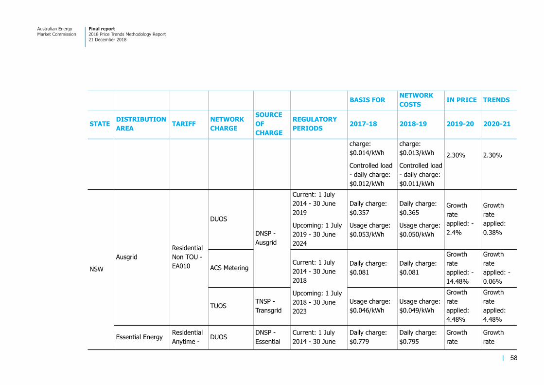
BASIS FORNETWORK


STATEDISTRIBUTION

AREATARIFF

NETWORK

CHARGE

SOURCE

OF

CHARGE

REGULATORY

PERIODS2017-18 2018-19 2019-20 2020-21

charge: $0.014/kWh


charge: $0.013/kWh


2.30% 2.30%

NSW

AusgridResidential Non TOU - EA010

DUOS

DNSP - Ausgrid









ACS MeteringCurrent: 1 July 2014 - 30 June 2018






TUOS TNSP - Transgrid





Essential Energy Residential Anytime - DUOS DNSP -

Essential Current: 1 July 2014 - 30 June



Growth rate

Growth rate

58



BASIS FORNETWORK


STATEDISTRIBUTION

AREATARIFF

NETWORK

CHARGE

SOURCE

OF

CHARGE

REGULATORY

PERIODS2017-18 2018-19 2019-20 2020-21

BLNN2AU

Energy

2019




applied: 1.98%

applied: 1.98%

ACS Metering Daily charge: $0.092











Endeavour EnergyResidential Block (anytime)

DUOSDNSP - Endeavour Energy













TUOS TNSP - Current: 1 July Usage chargeL Usage charge: Growth Growth

59



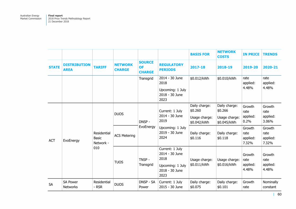
BASIS FORNETWORK


STATEDISTRIBUTION

AREATARIFF

NETWORK

CHARGE

SOURCE

OF

CHARGE

REGULATORY

PERIODS2017-18 2018-19 2019-20 2020-21

Transgrid 2014 - 30 June 2018


$0.012/kWh $0.010/kWh rate applied: 4.48%

rate applied: 4.48%

ACT EvoEnergy

Residential Basic Network - 010

DUOS

DNSP - EvoEnergy




















SA SA Power Networks

Residential - RSR DUOS DNSP - SA

Power Current: 1 July 2015 - 30 June



Growth rate

Nominally constant

60



BASIS FORNETWORK


STATEDISTRIBUTION

AREATARIFF

NETWORK

CHARGE

SOURCE

OF

CHARGE

REGULATORY

PERIODS2017-18 2018-19 2019-20 2020-21

Networks

2020




applied: 3.63%




Nominally constant

TUOS TNSP - ElectraNet







VIC Jemena

Residential - General Purpose - A100

DUOS

DNSP - Jemena

Current: 1 January 2016 - 31 December 2020

Upcoming: 1 January 2021 - 31 December 2025






Nominally constant




Nominally constant

TUOS TNSP - Current: 1 April Daily charge: Daily charge: Growth Growth

61



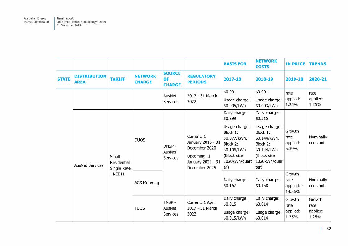
BASIS FORNETWORK


STATEDISTRIBUTION

AREATARIFF

NETWORK

CHARGE

SOURCE

OF

CHARGE

REGULATORY

PERIODS2017-18 2018-19 2019-20 2020-21

AusNet Services

2017 - 31 March 2022

$0.001


$0.001


rate applied: 1.25%

rate applied: 1.25%

AusNet Services

Small Residential Single Rate - NEE11

DUOSDNSP - AusNet Services




Usage charge: Block 1: $0.077/kWh, Block 2: $0.106/kWh (Block size 1020kWh/quarter)


Usage charge: Block 1: $0.144/kWh, Block 2: $0.144/kWh (Block size 1020kWh/quarter)


Nominally constant




Nominally constant

TUOSTNSP - AusNet Services

Current: 1 April 2017 - 31 March 2022




Usage charge: $0.014



62



BASIS FORNETWORK


STATEDISTRIBUTION

AREATARIFF

NETWORK

CHARGE

SOURCE

OF

CHARGE

REGULATORY

PERIODS2017-18 2018-19 2019-20 2020-21

United Energy

Low Voltage Small 1 Rate - LVS1R

DUOSDNSP - United Energy








Nominally constant




Nominally constant







CitipowerResidential Single Rate - C1R

DUOS

DNSP - Citipower








Nominally constant




Nominally constant

TUOS TNSP - Current: 1 April Usage charge: Usage charge: Growth Growth

63



BASIS FORNETWORK


STATEDISTRIBUTION

AREATARIFF

NETWORK

CHARGE

SOURCE

OF

CHARGE

REGULATORY

PERIODS2017-18 2018-19 2019-20 2020-21

AusNet Services

2017 - 31 March 2022 $0.018/kWh $0.018/kWh

rate applied: 1.25%

rate applied: 1.25%

PowercorResidential Single Rate - D1

DUOS

DNSP - Powercor








Nominally constant




Nominally constant







64



BASIS FORNETWORK


STATEDISTRIBUTION

AREATARIFF

NETWORK

CHARGE

SOURCE

OF

CHARGE

REGULATORY

PERIODS2017-18 2018-19 2019-20 2020-21

Tas TasNetworks

Residential LV General (Residential Light and Power) - TAS31 & Uncontrolled low voltage heating (Heating and hot water) - TAS41

DUOS

DNSP/TNSP: TasNetworks









ACS Metering

TAS31 - Daily charge: $0.061






TUOS






Usage charge: 0.075/kWh



NT Power and Water Corporation

For customers NUOS TNSP &

DNSP - Current: 1 July 2014 - 30 June



Nominally constant

Nominally constant

65



Source: AER Final and Draft Decision for regulatory periods, AER approved-Annual Pricing Proposals, ERA Final decision on Access Arrangement, jurisdictionally provided data. AEMC analysis. Note: Victorian prices are determined/changed on a calendar year basis and therefore 2017/-18 refers to 2018 and so on for Victorian transmission, distribution and metering charges.

BASIS FORNETWORK


STATEDISTRIBUTION

AREATARIFF

NETWORK

CHARGE

SOURCE

OF

CHARGE

REGULATORY

PERIODS2017-18 2018-19 2019-20 2020-21

with consumption below 750MWh per year - Schedule C

Power and Water Corporation

2019 Usage charge: $0.106/kWh


WA Western power

Anytime Energy (Residential) Exit Service - RT1

DUOS

TNSP & DNSP - Western Power








ACS Metering




TUOS Usage charge: $0.015/kWh




66

