2017 Cambridge - McKinsey Risk Prize Bio-sketch and

Photo Page

Student Name: Ashish Srivastava

Email contact: as2644@cam.ac.uk

Title of Submission: _________________________

Systemic Liquidity Risk: A Macroeconomic Evaluation

I am a candidate for the degree:

Master of Finance (M.Fin.)

Bio-sketch (Approximately 150 words)

Ashish Srivastava works for the Reserve Bank of India (RBI), India’s Central Bank since the

year 2006. Prior to joining the RBI, he was with the Food Corporation of India (FCI), a large

public sector organisation, for more than five years. A PhD in Working Capital

Management and MBA with specialization in Finance, he has qualified the eligibility test

for university lectureship in India and also has about three year’s university teaching

experience to his credit. His qualifications include the Certified Associate (CAIIB) and

Certificate in Treasury and Risk Management (CTRM) of the Indian Institute of Banking

and Finance (IIBF). He is a certified Financial Risk Manager (FRM) and has also obtained

the International Certificate in Banking Risk and Regulation (ICBRR) of the Global

Association of Risk Professionals (GARP), USA. He has been sponsored by his employer for

the master of finance (M.Fin.) degree programme at the CJBS, University of Cambridge.

Systemic Liquidity Risk: A Macroeconomic Evaluation

Ashish Srivastava MFin (Class of 2016)

Cambridge Judge Business School Churchi l l College, University of Cambridge

Cambridge

as2644@cam.ac.uk

JEL Classification: E02, E51, E58, G21, G32.

Key Words: Macro-economy, Money Supply, Central Banking, Banks, Risk.

The views are personal and do not necessarily reflect those of the Reserve Bank of India.

All the data is sourced from the database on India Economy, Reserve Bank of India.

https://dbie.rbi.org.in/DBIE/dbie.rbi?site=home

2017 Cambridge - McKinsey Risk Prize Declaration Form

Student Name: Ashish Srivastava

Email contact: as2644@cam.ac.uk

Title of Submission: _______________________________________

Systemic Liquidity Risk: A Macroeconomic Evaluation

Number of words of submission: 3687

I am a candidate for the degree: M.Fin.

Academic Institution/Department: CJBS

Declaration

I confirm that this piece of work is my own and does not violate the University of Cambridge Judge Business School’s guidelines on Plagiarism.

I agree that my submission will be available as an internal document for members of both Cambridge Judge Business School and McKinsey & Co’s Global Risk Practice.

If my submission either wins or receives an honourable mention for the Risk Prize, then I agree that (a) I will be present at the award presentation ceremony on 23 June 2017, (b) my submission can be made public on a Cambridge Judge Business School and/or McKinsey & Co websites.

This submission on risk management does not exceed 10 pages.

Signed (Electronic Signature)

March 01, 2017

1

Systemic Liquidity Risk: A Macroeconomic Evaluation

Paper Snapshot

Abstract

The likelihood of not getting the desired funding at an

appropriate cost or the probability of bearing an undue

loss of value in a fire sale is recognised as the liquidity risk.

However, a flat idiosyncratic liquidity risk does not

necessarily translate into a similar risk neutral position at

the systemic level. Systemic liquidity risk emanates from

the underestimation and imprecise understanding of the

liquidity conundrum and its causal relationship with the

exogenous or endogenous factors. Systemic risk finally

devolves at the macro level with serious repercussions.

This paper attempts a macroeconomic evaluation of the

systemic liquidity risk from the perspective of developing

economies. As a test case, the relevant macroeconomic

data from the Indian financial system has been used for

the purpose of analysis, modelling and interpretation.

JEL Classification

E02, E51, E58, G21, G32

Keywords

Macro-economy, Money-

Supply, Central Banking,

Banks, Risk

1. Introduction

Systemic liquidity risk has attracted the attention of the financial sector beyond the

corridors of central banking, especially in the aftermath of the global financial crisis.

However, it has not gained as much significance in the spectrum of risk management as it

should have given the enormity of its impact and it has continued to be seen as a monetary

policy or lender of last resort (LOLR) function. The challenge posed by the systemic liquidity

risk is that even perfectly rational liquidity management decisions taken at the level of an

individual financial institution could prove hazardous at the systemic level. Hence, it is

important to understand the causal relationships between the macroeconomic variables

impinging upon the systemic liquidity. There is an ongoing debate on how to adequately

address the systemic component of the liquidity risk and a number of researchers have

studied its various dimensions. Maddaloni (2015) noted that the risk stemming from the

bank’s liquidity management inefficiency or strategic liquidity management decisions has a

bearing on the systemic level. Ratnovski (2009) examined the factors shaping the resilience

of Canadian banks and noted that less reliance on wholesale funding than their peers in

other advanced countries helped them. Demirguc-Kunt and Huizinga (2009) found that the

banks’ reliance on non-deposit sources of funds made them more vulnerable. Rajan (2006)

observed that that banks’ greater reliance on market liquidity caused risk to their balance

sheets in times of crisis.

While at the idiosyncratic level a number of factors could be responsible for a bank’s specific

liquidity crunch, it is far more important and useful to understand the manifestation of the

liquidity risk at the systemic level. The challenge is to use and relate the macroeconomic

2

data to understand and mitigate the liquidity conundrum. In general, the systemic liquidity

management resonates between absorption and injections as conditions evolve from

surplus and shortage at the macro level. A macroeconomic evaluation of systemic liquidity

risk from the perspective of developing economies, therefore, hinges upon the following

four risk parameters.

Frictional liquidity risk occurs due to the interaction between the transient factors, such

as periodic tax collections, volatile government receipts, large one-time

receipts/payments or inflationary spirals.

Structural liquidity risk is caused by the widening difference between the credit pick-up

and the deposit growth in the banking system coupled with the movement in the

currency in circulation.

Funding liquidity risk is the risk that the counterparties who provide the short-term

funding might withdraw or not roll-over the funding.

Market liquidity risk is the risk of a generalised disruption in asset markets thereby

making otherwise apparently liquid assets illiquid.

The frictional and structural liquidity risks are manifested in the form of funding liquidity risk

and also the market liquidity risk. Both of these could precede and succeed each other

depending upon the prevailing macroeconomic scenario. Interactions of the above four risk

parameters define and shape the liquidity risk at the systemic level.

2. Systemic liquidity

The maintenance of an adequate level of systemic liquidity consistent with its ultimate goals

of price and financial stability is of paramount importance for an economy. At the same time,

it is also critical that the banks and financial institutions adopt prudent liquidity management

systems and have adequate liquidity buffers to ward off any possible liquidity crisis; as the

huge reputational risk that is propagated by the liquidity crisis could have serious negative

repercussions for financial stability. Figure 1 presents a schematic view of the manifestation

of systemic liquidity risk.

Figure 1: A Schematic View of the Systemic Liquidity Risk

3

The macroeconomic factors affecting the systemic liquidity scenario could emerge from

exogenous shocks or endogenous imbalances. While the exogenous shocks of the magnitude

of the global financial crisis of 2008 could seriously threaten liquidity in the affected

economies, even the endogenous imbalances prevailing in the financial system could also

jeopardise the financial stability and systemic liquidity equilibrium. Though the manifestation

of systemic liquidity risk could take different forms and patterns, the systemic liquidity risk

and threat to financial stability become more pronounced both in the case of recession

(rather a depression) and hyperinflation.

The liquidity conundrum is manifested both in the case of sudden shrinkage in the economic

activities, as explained above in the case of external shocks. In this situation, the systemic

liquidity risk originates from a worsening of the market liquidity which leads to funding

liquidity risk and subsequently assumes the structural dimension. Due to the limited role of a

frictional component of liquidity risk, in this case, the job of restoring normalcy becomes quite

tedious for the central bank. While the short-term liquidity adjustment by the central bank

could manage the frictional nature of the liquidity risk by, the structural dimension of

systemic liquidity risk demands enduring management and also active support from the fiscal

front. A more challenging and rather subtle form of systemic liquidity risk stems from an

overheating economy, especially when the source of overheating is centred on the

comparative illiquid asset classes, such as property, gold or other speculative investments. In

the context of developing economies, a certain involvement of the so-called black money also

plays a hand in the overpricing of assets and under-pricing or risks. Apparently, this signals a

false impression of growth, but in reality, this brings in a vicious cycle of poor credit. Such a

vicious cycle severely impacts the banks and borrowers alike. A hardening of interest rates

leads to shrinkage of funding liquidity which then spills over to the market liquidity risk.

Though the liquidity conundrum, in this case, remains mostly frictional, if sustained, it could

also assume a structural dimension. Systemically important financial institutions (SIFI) play a

critical role in the entire episode along with the monetary and fiscal stance. Policy

transmission mostly happens through interest rates and asset price channels with their

natural time-lags. It is important, therefore, to understand the macroeconomic factors which

could be monitored to assess the liquidity risk at the systemic level.

The unsecured segment of the inter-bank call money market sets the weighted average call

rate (WACR) on a daily basis, which is the operating target of monetary policy in India

(Pattanaik and Kavediya, Rajesh, 2017) and hence, could be used as a proxy indicator for

liquidity risk. By modulating liquidity conditions, the Reserve Bank of India (RBI) aims to

anchor the WACR around the policy repo rate and therefore the movement of WACR above

the policy repo rate could be used an indicator of liquidity stress at the systemic level. An

excess of WACR over the repo rate could be considered as the liquidity risk premium.

In case the WACR is used as the dependent variable as a proxy indicator for liquidity risk, the

choice of independent factors (variables) should be the most relevant macroeconomic factors

4

defining all the four components of systemic liquidity, namely, structural, frictional, market,

and funding liquidity. To illustrate, variables defining the structural liquidity, such as credit

growth, deposit growth, reserve money growth, frictional liquidity (such as bank and central

government cash balances), market liquidity (such as gold, property, stock prices, as also the

wholesale price growth), and funding liquidity (such as repo rate), benchmark 10-year

government bond yield, etc. could be used as independent variables having an influence over

the WACR, the dependent variable. The impact of repo operations under the LAF, though

quite important, is expressed in the frictional liquidity variables and hence, should not be

used as an independent variable.

It could be observed from Figure 2 that during the last five years, the WACR has mostly

remained aligned with the policy repo rate, except for occasional liquidity spikes and a period

of liquidity stress during July – December 2013 when the WACR substantially moved upward,

notwithstanding the heavy injection of liquidity under the LAF. On a long term basis, the

systemic liquidity risk was contained around the policy corridor and the periods of liquidity

stress were characterised by macroeconomic issues, such as inflationary pressures and

volatility in the foreign exchange market. During the recent past, the LAF has mostly remained

in absorption mode and the call rates not only fell in line with the policy repo rates but were

hovering slightly below the policy rates, indicating a comfortable position of the systemic

liquidity. One of the major macroeconomic factors responsible for such a cushion was possibly

the high-value banknote demonetisation move by the Government of India on 8 November

2016, thereby demonstrating the impact of macroeconomic factors on systemic liquidity.

However, this is not to suggest that the institution-specific factors do not impact on liquidity

at the systemic level. For instance, in India, the final guidelines1 on the Liquidity Coverage

1 LCR guidelines, Reserve Bank of India - https://rbidocs.rbi.org.in/rdocs/content/pdfs/CA09062014_A.pdf

-4,000.00

-3,000.00

-2,000.00

-1,000.00

0.00

1,000.00

2,000.00

3,000.00

4,000.00

5.00

5.50

6.00

6.50

7.00

7.50

8.00

8.50

9.00

9.50

10.00

10.50

11.00

2 N

ov

20

12

2 J

an 2

01

3

2 M

ar 2

01

3

2 M

ay 2

01

3

2 J

ul 2

01

3

2 S

ep 2

01

3

2 N

ov

20

13

2 J

an 2

01

4

2 M

ar 2

01

4

2 M

ay 2

01

4

2 J

ul 2

01

4

2 S

ep 2

01

4

2 N

ov

20

14

2 J

an 2

01

5

2 M

ar 2

01

5

2 M

ay 2

01

5

2 J

ul 2

01

5

2 S

ep 2

01

5

2 N

ov

20

15

2 J

an 2

01

6

2 M

ar 2

01

6

2 M

ay 2

01

6

2 J

ul 2

01

6

2 S

ep 2

01

6

2 N

ov

20

16

2 J

an 2

01

7

LAF

Vo

lum

e (

Rs.

Bn

)

WA

CR

/Po

licy

Re

po

Rat

e (

%)

Period

LAF -Net liquidity injection(+)/absorption(-) (Rs Bn) Call Money Rate (Weighted Average %) Policy Repo Rate (%)

Figure 2: WACR, Repo Rate, and LAF Volume

5

5.5

6

6.5

7

7.5

8

8.5

9

9.5

10

10.5 11

11.5

12

Dec

. 30

, 20

11

Feb

. 17

, 20

12

Ap

r. 6

, 20

12

May

25

, 20

12

Jul.

13

, 20

12

Au

g. 3

1, 2

01

2

Oct

. 19

, 20

12

Dec

. 7, 2

01

2

Jan

. 25

, 20

13

Mar

. 15

, 20

13

May

3, 2

01

3

Jun

. 21

, 20

13

Au

g. 9

, 20

13

Sep

. 27

, 20

13

No

v. 1

5, 2

01

3

Jan

. 3, 2

01

4

Feb

. 21

, 20

14

Ap

r. 1

1, 2

01

4

May

30

, 20

14

Jul.

18

, 20

14

Sep

. 5, 2

01

4

Oct

. 24

, 20

14

Dec

. 12

, 20

14

Jan

. 30

, 20

15

Mar

. 20

, 20

15

May

8, 2

01

5

Jun

. 26

, 20

15

Au

g. 1

4, 2

01

5

Oct

. 2, 2

01

5

No

v. 2

0, 2

01

5

Jan

. 8, 2

01

6

Feb

. 26

, 20

16

Ap

r. 1

5, 2

01

6

Jun

. 3, 2

01

6

Jul.

22

, 20

16

Sep

. 9, 2

01

6

Oct

. 28

, 20

16

Dec

. 16

, 20

16

Inte

rest

rat

e (

%)

Call Money Rate (Weighted Average) 91-Day Treasury Bill (Primary) Yield

10-Year Government Securities Yield

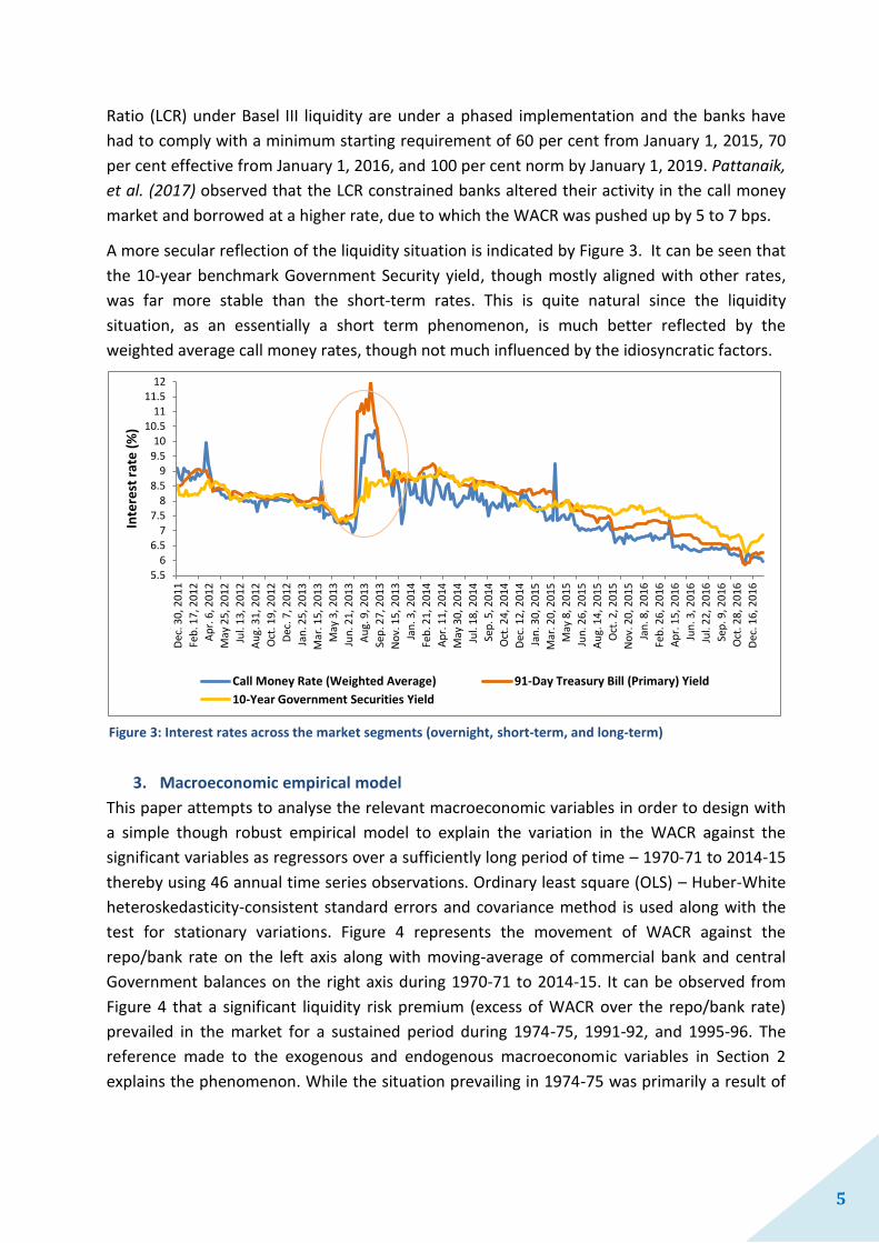
Ratio (LCR) under Basel III liquidity are under a phased implementation and the banks have

had to comply with a minimum starting requirement of 60 per cent from January 1, 2015, 70

per cent effective from January 1, 2016, and 100 per cent norm by January 1, 2019. Pattanaik,

et al. (2017) observed that the LCR constrained banks altered their activity in the call money

market and borrowed at a higher rate, due to which the WACR was pushed up by 5 to 7 bps.

A more secular reflection of the liquidity situation is indicated by Figure 3. It can be seen that

the 10-year benchmark Government Security yield, though mostly aligned with other rates,

was far more stable than the short-term rates. This is quite natural since the liquidity

situation, as an essentially a short term phenomenon, is much better reflected by the

weighted average call money rates, though not much influenced by the idiosyncratic factors.

3. Macroeconomic empirical model

This paper attempts to analyse the relevant macroeconomic variables in order to design with

a simple though robust empirical model to explain the variation in the WACR against the

significant variables as regressors over a sufficiently long period of time – 1970-71 to 2014-15

thereby using 46 annual time series observations. Ordinary least square (OLS) – Huber-White

heteroskedasticity-consistent standard errors and covariance method is used along with the

test for stationary variations. Figure 4 represents the movement of WACR against the

repo/bank rate on the left axis along with moving-average of commercial bank and central

Government balances on the right axis during 1970-71 to 2014-15. It can be observed from

Figure 4 that a significant liquidity risk premium (excess of WACR over the repo/bank rate)

prevailed in the market for a sustained period during 1974-75, 1991-92, and 1995-96. The

reference made to the exogenous and endogenous macroeconomic variables in Section 2

explains the phenomenon. While the situation prevailing in 1974-75 was primarily a result of

Figure 3: Interest rates across the market segments (overnight, short-term, and long-term)

6

0.00 250.00 500.00 750.00 1000.00 1250.00 1500.00 1750.00 2000.00 2250.00 2500.00 2750.00 3000.00 3250.00 3500.00 3750.00 4000.00 4250.00 4500.00 4750.00 5000.00

2.0

4.0

6.0

8.0

10.0

12.0

14.0

16.0

18.0

20.0

22.0

19

70

-71

19

72

-73

19

74

-75

19

76

-77

19

78

-79

19

80

-81

19

82

-83

19

84

-85

19

86

-87

19

88

-89

19

90

-91

19

92

-93

19

94

-95

19

96

-97

19

98

-99

20

00

-01

20

02

-03

20

04

-05

20

06

-07

20

08

-09

20

10

-11

20

12

-13

20

14

-15

C

om

m. b

anks

/Go

vt B

alan

ces

(Rs.

Bn

)

Rat

e (

%)

Year

Comm_Bank_Bal_M_AV C_Govt_Bal_M_AV Repo/Bank Rate WACR

external oil price shock2, the later periods of liquidity stress were the manifestations of

internal imbalances in the economy (the BoP crisis3). A rapid monetization of the economy

during the last 15 years is also apparent.

Model Estimation - A number of critical macroeconomic variables were examined to develop

a suitable regression model to establish a causal relationship and find useful explanations

about the systemic liquidity risk. Some of the variables, such as the gross fiscal deficit, current

account deficit, growth in capital, and gold and illiquid asset prices were initially considered

but were not found significant, either due to strong multicollinearity with other independent

variables or due to a lack of comparable data. After examining the suitability of various

estimation variables, the following model was developed as a simple, robust and significant

causal OLS regression model. An explanation of the variables is as follows –

CALL_WTD = Weighted average interbank call money interest rate (WACR)

M0_GR = Annual growth in the reserve money (%) (Currency in circulation + banker’s deposits with the RBI + other (FI) deposits with RBI)

WPI_GR = Annual growth in the wholesale price index (%) (Proxy for inflation)

CRR = Cash Reserve Ratio (%)4

SLR = Statutory Liquidity Ratio (%)5

CR_GR = Annual growth in the commercial bank’s credits (%)

DEP_GR = Annual growth in the commercial bank’s deposits (%)

2 Production cuts by the OAPEC had nearly quadrupled the oil prices in January 1974. 3 India faced a serious Balance of Payment (BoP) crisis during 90s necessitating pledge of gold to get IMF funding.

4 Cash Reserve Ratio (CRR) as prescribed by the RBI is mandated for commercial banks u/s 42 of R.B.I. Act (1934).

5 Statutory Liquidity Ratio (SLR) as prescribed by the RBI is mandated for comm. banks u/s 24 of B.R. Act (1949).

Figure 4: WACR, Repo Rates, Moving Average - Commercial banks and Central Govt. Balances (Rs. Bn)

7

Considering the nature of variation and data generating process, a non-linear cubic variable

transformation was attempted in respect of variation in the wholesale price index and an

interaction between deposit growth and credit growth rates was used as regressors. The

following are the estimation equation, the substituted coefficients and the OLS table.

Estimation Equation:

CALL_WTD = C(1) + C(2)*M0_GR + C(3)*WPI_GR + C(4)*(WPI_GR)^2 + C(5)*(WPI_GR)^3 +

C(6)*CRR + C(7)*SLR + C(8)*(DEP_GR)/(CR_GR) + C(9)*CR_GR + C(10)*DEP_GR

Substituted Coefficients:

CALL_WTD = 10.21 - 0.09*M0_GR + 0.01*WPI_GR - 0.02*(WPI_GR)^2 + 0.001*(WPI_GR)^3 +

0.49*CRR + 0.19*SLR - 7.50*(DEP_GR)/(CR_GR) - 0.36*CR_GR + 0.30*DEP_GR

Dependent Variable: CALL_WTD Method: Least Squares Sample: 1 21 23 46 Included observations: 45 White heteroskedasticity-consistent standard errors & covariance

CALL_WTD = Weighted Average Call Rate (WACR) used as an indicator of systemic liquidity risk.

Variable Coefficient Std. Error t-Statistic Prob. Residue Plot C 10.20574 2.749638 3.711668 0.0007

M0_GR -0.093032 0.038021 -2.446891 0.0196 WPI_GR 0.010980 0.144422 0.076026 0.9398

(WPI_GR)^2 -0.021098 0.017321 -1.218088 0.2313 (WPI_GR)^3 0.000972 0.000523 1.857613 0.0717

CRR 0.485969 0.105479 4.607252 0.0001 SLR 0.186775 0.049283 3.789825 0.0006

(DEP_GR)/(CR_GR) -7.495016 1.779948 -4.210805 0.0002 CR_GR -0.362030 0.084532 -4.282770 0.0001

DEP_GR 0.298037 0.115327 2.584279 0.0141 R-squared 0.672143 Mean dependent var 8.479556

Adjusted R-squared 0.587837 S.D. dependent var 2.851269 S.E. of regression 1.830512 Akaike info criterion 4.240198 Sum squared resid 117.2771 Schwarz criterion 4.641679 Log likelihood -85.40447 Hannan-Quinn criter. 4.389866 F-statistic 7.972662 Durbin-Watson stat 1.834103 Prob(F-statistic) 0.000003 Wald F-statistic 16.44644 Prob(Wald F-statistic) 0.000000

Ramsey RESET Test Omitted Variables: Powers of fitted values from 2 to 3

Value df Probability

F-statistic 1.594027 (2, 33) 0.2184

Likelihood ratio 4.149969 2 0.1256

8

0.25

0.50

0.75

1.00

1.25

1.50

1.75

2.00

2.25

2.50

19

70

-71

19

72

-73

19

74

-75

19

76

-77

19

78

-79

19

80

-81

19

82

-83

19

84

-85

19

86

-87

19

88

-89

19

90

-91

19

92

-93

19

94

-95

19

96

-97

19

98

-99

20

00

-01

20

02

-03

20

04

-05

20

06

-07

20

08

-09

20

10

-11

20

12

-13

20

14

-15

Rat

io o

f D

ep

osi

t to

Cre

dit

Gro

wth

Period

Deposit Growth/Credit Growth

4. Model interpretation

The overall model is significant. The F-statistic is 7.98 and its P-value is 0.000003, which is

much smaller than 0.05. All the variables including the intercept are significant at 5% except

for the cubic transformation of WPI_Gr, which is significant at 10%. The P-value of the Wald F-

statistic is 0.00 and hence, all the variables are jointly significant. R2 of 0.67 indicates that

about 67% of the total variation in WACR is explained by the model. Adjusted R2 of 0.59 is not

too far from the R2 and hence, the inclusion of additional regressors has not reduced the

explanatory capabilities of the model. The SER at 1.83 is lower than the SD of the dependent

variable at 2.85. Based on the influence statistic, one of the most influential observations was

omitted so as to ensure a fair estimate. The residue appears to be evenly distributed within

the 95% confidence ellipse across the fitted WACR and hence, meets the requirement of a

zero conditional mean for OLS estimation. The model also passes the functional form (Ramsey

RESET) test – the P-value of F-statistic is 0.22, well above the significance level of 5%.

The model provides a very useful insight into the causal relationship of systemic liquidity to

significant macroeconomic variables. An expansion of 1% in the reserve money (M0) reduces

the WACR by 0.09%. An increase of 1% in both the CRR and SLR reduces the liquidity and adds

0.49% and 0.19% to the WACR, cetaris paribus, respectively. A very interesting inference is

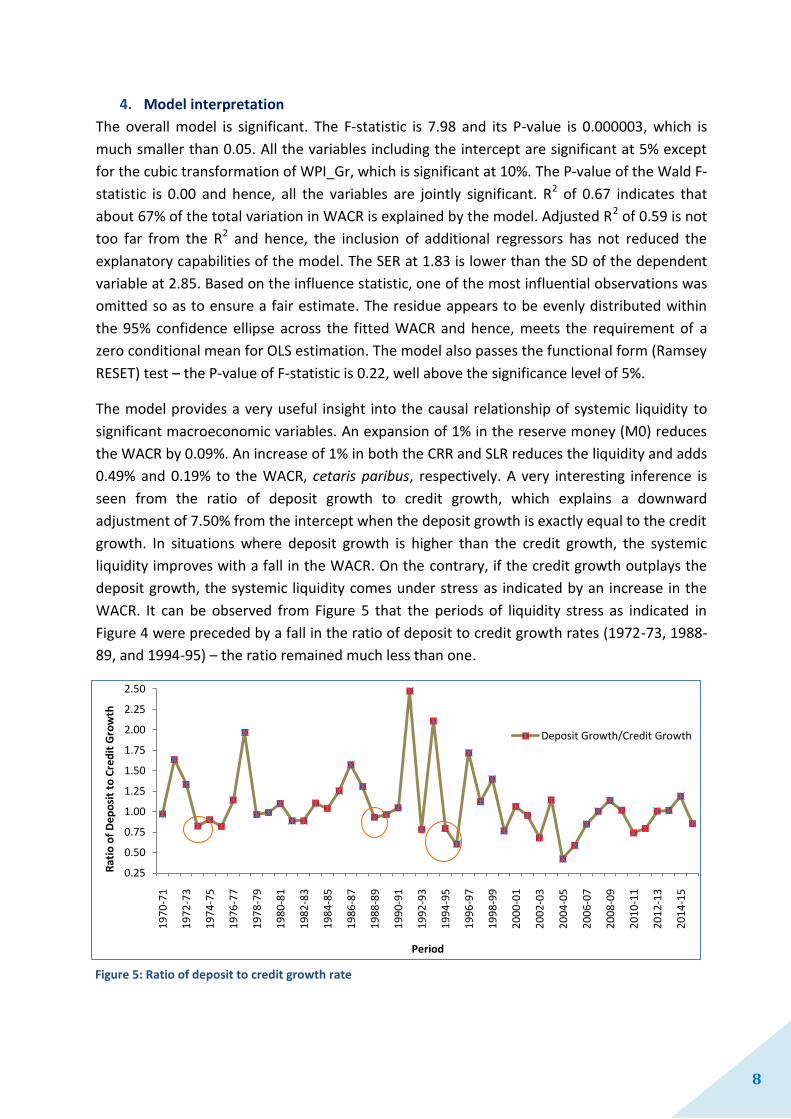
seen from the ratio of deposit growth to credit growth, which explains a downward

adjustment of 7.50% from the intercept when the deposit growth is exactly equal to the credit

growth. In situations where deposit growth is higher than the credit growth, the systemic

liquidity improves with a fall in the WACR. On the contrary, if the credit growth outplays the

deposit growth, the systemic liquidity comes under stress as indicated by an increase in the

WACR. It can be observed from Figure 5 that the periods of liquidity stress as indicated in

Figure 4 were preceded by a fall in the ratio of deposit to credit growth rates (1972-73, 1988-

89, and 1994-95) – the ratio remained much less than one.

Figure 5: Ratio of deposit to credit growth rate

9

-0.2

-0.1

0.0

0.1

0.2

0.3

0.4

-6.0

-5.3

-4.6

-3.9

-3.2

-2.5

-1.8

-1.1

-0.4

0.3

1.0

1.7

2.4

3.1

3.8

4.5

5.2

5.9

6.6

7.3

8.0

8.7

9.4

10

.1

10

.8

11

.5

12

.2

12

.9

13

.6

14

.3

15

.0

15

.7

16

.4

17

.1

17

.8

Ch

ange

in W

AC

R (

%)

Change in WPI (%)

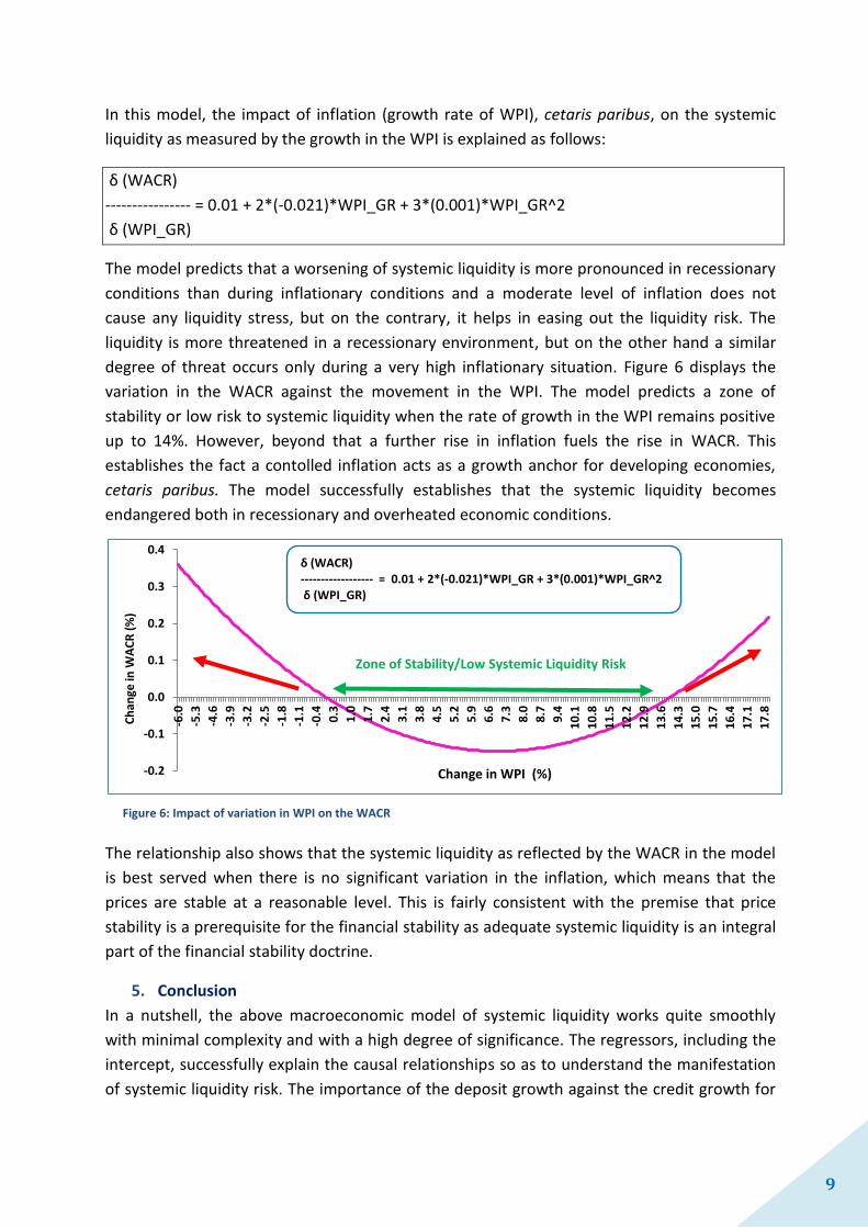
δ (WACR) ------------------ = 0.01 + 2*(-0.021)*WPI_GR + 3*(0.001)*WPI_GR^2 δ (WPI_GR)

In this model, the impact of inflation (growth rate of WPI), cetaris paribus, on the systemic

liquidity as measured by the growth in the WPI is explained as follows:

δ (WACR)

---------------- = 0.01 + 2*(-0.021)*WPI_GR + 3*(0.001)*WPI_GR^2

δ (WPI_GR)

The model predicts that a worsening of systemic liquidity is more pronounced in recessionary

conditions than during inflationary conditions and a moderate level of inflation does not

cause any liquidity stress, but on the contrary, it helps in easing out the liquidity risk. The

liquidity is more threatened in a recessionary environment, but on the other hand a similar

degree of threat occurs only during a very high inflationary situation. Figure 6 displays the

variation in the WACR against the movement in the WPI. The model predicts a zone of

stability or low risk to systemic liquidity when the rate of growth in the WPI remains positive

up to 14%. However, beyond that a further rise in inflation fuels the rise in WACR. This

establishes the fact a contolled inflation acts as a growth anchor for developing economies,

cetaris paribus. The model successfully establishes that the systemic liquidity becomes

endangered both in recessionary and overheated economic conditions.

The relationship also shows that the systemic liquidity as reflected by the WACR in the model

is best served when there is no significant variation in the inflation, which means that the

prices are stable at a reasonable level. This is fairly consistent with the premise that price

stability is a prerequisite for the financial stability as adequate systemic liquidity is an integral

part of the financial stability doctrine.

5. Conclusion

In a nutshell, the above macroeconomic model of systemic liquidity works quite smoothly

with minimal complexity and with a high degree of significance. The regressors, including the

intercept, successfully explain the causal relationships so as to understand the manifestation

of systemic liquidity risk. The importance of the deposit growth against the credit growth for

Figure 6: Impact of variation in WPI on the WACR

Zone of Stability/Low Systemic Liquidity Risk

10

systemic liquidity is highly relevant from the perspective of developing economies. Moreover,

the model at 10% significance demonstrates that the systemic liquidity risk could be mitigated

to a large extent by ensuring the price stability. Since other significant variables, namely the

CRR and SLR are used as policy tools to ensure price stability; a lower systemic liquidity risk

premium depends to a great extent on the stable prices and well anchored inflationary

expectations. To summarise, this paper shows that the structural and frictional liquidity risks

shape the systemic liquidity risk through the channels of funding and market liquidity risk. It is

therefore; quite useful both for the market participants and the central bank to keep a close

watch on the interaction among these risk parameters so as to better understand and

mitigate the manifestation of systemic liquidity risk.

6. Scope for further work

Figure 7 shows that a lower cash to deposit ratio (right axis) could also help in lowering the

systemic liquidity risk, though a precise causal relationship is not known. Secondly, a high

level of aggregate bank reserves may not necessarily help in smoothing the liquidity shock. A

fall in cash to GDP ratio could also be an important factor in this arena. There is scope for

further empirical work relating to the impact of these factors on the systemic liquidity risk.

Figure 7: Impact of additional macroeconomic factors on the systemic liquidity risk

References 1. De Nicoló, M.G., Favara, G., Ratnovski, L., 2012. Externalities and macroprudential policy. International

Monetary Fund.

2. Demirgüç-Kunt, A., Huizinga, H., 2010. Bank activity and funding strategies: The impact on risk and returns.

Journal of Financial Economics 98, 626–650.

3. Maddaloni, G., 2015. Liquidity risk and policy options. Journal of Banking & Finance 50, 514–527.

doi:10.1016/j.jbankfin.2014.01.018

4. Pattanaik, S., Kavediya, Rajesh, H., Angshuman, 2017. The Unintended Side Effects of Basel III Liquidity

Regulations on the Operating Target of Monetary Policy (Working Paper No. WPS (DEPR): 02 / 2017), WPS

(DEPR). Reserve Bank of India, Mumbai.

5. Rajan, R.G., 2006. Has finance made the world riskier? European Financial Management 12, 499–533.

6. Reserve Bank of India, 2014. Report of the Expert Committee to Revise and Strengthen the Monetary Policy

Framework. Reserve Bank of India, Mumbai.

0.0

10.0

20.0

30.0

40.0

50.0

60.0

70.0

80.0

0.0 2.0 4.0 6.0 8.0

10.0 12.0 14.0 16.0 18.0 20.0

19

70

-71

19

72

-73

19

74

-75

19

76

-77

19

78

-79

19

80

-81

19

82

-83

19

84

-85

19

86

-87

19

88

-89

19

90

-91

19

92

-93

19

94

-95

19

96

-97

19

98

-99

20

00

-01

20

02

-03

20

04

-05

20

06

-07

20

08

-09

20

10

-11

20

12

-13

20

14

-15

Cas

h t

o D

ep

osi

ts (

%)

Pe

rce

nta

ge

Period

Cash to GDP (current prices) Ratio (%) Cash to Aggregate Deposits (%) Bank Reserves (Balances with RBI plus Cash with Banks)/ Aggregate Deposits(%) Repo/Bank Rate