2017- 2018 computational mathematics and … ppt_5.pdfcomputational mathematics and integral...

COMPUTATIONAL MATHEMATICS

AND

INTEGRAL CALCULUS

Institute of Aeronautical Engineering

2017- 2018

Prepared by

Ms. P.Rajani

Associate Professor

Freshman Engineering

COMPUTATIONAL MATHEMATICS AND INTEGRAL CALCULUS

(CMIC)

• Root finding techniques

• Interpolation

• Curve fitting

• Numerical solutions of ordinary differential equations

• Multiple integrals

• Vector calculus

• Gamma function

• Bessel’s function

CONTENTS

TEXT BOOKS

• Advanced Engineering Mathematics by

Kreyszig, John Wiley & Sons.

• Higher Engineering Mathematics by Dr. B.S. Grewal, Khanna Publishers

REFERENCES

• R K Jain, S R K Iyengar, “Advanced

Engineering Mathematics”, Narosa

Publishers, 5th Edition, 2016.

• S. S. Sastry, “Introduction Methods of

Numerical Analysis”, Prentice-Hall of India Private Limited, 5th Edition, 2012.

WEB REFERENCES

• http://www.efunda.com/math/math_home/math.cfm

• http://www.ocw.mit.edu/resources/#Mathematics

• http://www.sosmath.com/

• http://www.mathworld.wolfram.com

E-TEXT BOOKS

• http://www.keralatechnologicaluniversity.blogspot.in/2015/06/erwin-kreyszig-advanced-engineeringmathematics-ktu-ebook-download.html

• http://www.faadooengineers.com/threads/13449-Engineering-Maths-II-eBooks

ROOT F INDING TECHNIQUES AND INTERPOLAT ION

UNIT-I

ROOT FINDING TECHNIQUES

BISECTION METHOD

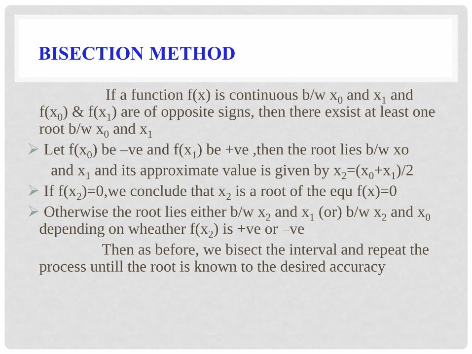
If a function f(x) is continuous b/w x0 and x1 and f(x0) & f(x1) are of opposite signs, then there exsist at least one root b/w x0 and x1

Let f(x0) be –ve and f(x1) be +ve ,then the root lies b/w xo

and x1 and its approximate value is given by x2=(x0+x1)/2

If f(x2)=0,we conclude that x2 is a root of the equ f(x)=0

Otherwise the root lies either b/w x2 and x1 (or) b/w x2 and x0 depending on wheather f(x2) is +ve or –ve

Then as before, we bisect the interval and repeat the process untill the root is known to the desired accuracy

REGULA-FALSI

The idea for the Regula-Falsi method is to connect the points (a,f(a)) and

(b,f(b)) with a straight line.Since linear equations are the simplest equations to

solve for find the regula-falsi point (xrfp) which is the solution to the linear

equation connecting the endpoints.

Look at the sign of f(xrfp):

If sign(f(xrfp)) = 0 then end algorithm

else If sign(f(xrfp)) = sign(f(a)) then set a = xrfp

else set b = xrfp

x-axis a b

f(b)

f(a) actual root

f(x)

xrfp

equation of line:

axab

afbfafy

)()()(

solving for xrfp

)()(

)(

)()(

)(

)()()(0

afbf

abafax

axafbf

abaf

axab

afbfaf

rfp

rfp

rfp

NEWTON-RAPHSON METHOD OR NEWTON ITERATION METHOD

Let the given equation be f(x)=0

Find f1(x) and initial approximation x0

The first approximation is x1= x0-f(x0)/ f1(x0)

The second approximation is x2= x1-f(x1)/ f1(x1)

.

.

The nth approximation is xn= xn-1-f(xn)/ f1(xn)

)(xfy

0x1x

),( 00 yx x

INTERPOLATION

INTERPOLATION : The process of finding a

missed value in the given table values of X, Y.

FINITE DIFFERENCES : We have three finite

differences

1. Forward Difference

2. Backward Difference

3. Central Difference

FINITE DIFFERENCE METHODS

Let (xi,yi),i=0,1,2…………..n be the equally spaced data of the

unknown function y=f(x) then much of the f(x) can be extracted by analyzing

the differences of f(x).

Let x1 = x0+h

x2 = x0+2h

.

.

.

xn = x0+nh be equally spaced points where the function value of f(x)

be y0, y1, y2…………….. yn

SYMBOLIC OPERATORS

Forward shift operator(E) :

It is defined as Ef(x)=f(x+h) (or) Eyx = yx+h

The second and higher order forward shift operators are defined

in similar manner as follows

E2f(x)= E(Ef(x))= E(f(x+h)= f(x+2h)= yx+2h

E3f(x)= f(x+3h)

.

.

Ekf(x)= f(x+kh)

BACKWARD SHIFT OPERATOR(E-1) : It is defined as E-1f(x)=f(x-h) (or) Eyx = yx-h

The second and higher order backward shift operators are defined in similar manner as follows

E-2f(x)= E-1(E-1f(x))= E-1(f(x-h)= f(x-2h)= yx-2h

E-3f(x)= f(x-3h)

. . E-kf(x)= f(x-kh)

FORWARD DIFFERENCE OPERATOR (∆) :

The first order forward difference operator of a function f(x) with increment h in x is given by

∆f(x)=f(x+h)-f(x) (or) ∆fk =fk+1-fk ; k=0,1,2………

∆2f(x)= ∆[∆f(x)]= ∆[f(x+h)-f(x)]= ∆fk+1- ∆fk ; k=0,1,2…………

…………………………….

…………………………….

Relation between E and ∆ :

∆f(x)=f(x+h)-f(x)

=Ef(x)-f(x) [Ef(x)=f(x+h)]

=(E-1)f(x)

∆=E-1 E=1+ ∆

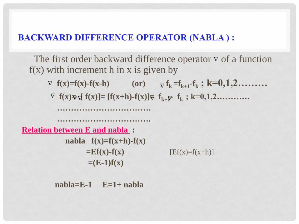
BACKWARD DIFFERENCE OPERATOR (NABLA ) :

The first order backward difference operator of a function f(x) with increment h in x is given by

f(x)=f(x)-f(x-h) (or) fk =fk+1-fk ; k=0,1,2………

f(x)= [ f(x)]= [f(x+h)-f(x)]= fk+1- fk ; k=0,1,2…………

…………………………….

…………………………….

Relation between E and nabla :

nabla f(x)=f(x+h)-f(x)

=Ef(x)-f(x) [Ef(x)=f(x+h)]

=(E-1)f(x)

nabla=E-1 E=1+ nabla

CENTRAL DIFFERENCE OPERATOR

The central difference operator is defined as

δf(x)= f(x+h/2)-f(x-h/2)

δf(x)= E1/2f(x)-E-1/2f(x)

= [E1/2-E-1/2]f(x)

δ= E1/2-E-1/2

RELATIONS BETWEEN THE OPERATORS IDENTITIES

1. ∆=E-1 or E=1+ ∆

2. = 1- E -1

3. δ = E 1/2 – E -1/2

4. µ= ½ (E1/2-E-1/2)

5. ∆=E = E= δE1/2

6. (1+ ∆)(1- )=1

NEWTONS INTERPOLATION FORMULA

•

GAUSS INTERPOLATION

The Guass forward interpolation is given by yp = yo

+ p ∆y0+p(p-1)/2! ∆2y-1 +(p+1)p(p-1)/3! ∆3y-

1+(p+1)p(p-1)(p-2)/4! ∆4y-2+……

The Guass backward interpolation is given by

yp = yo + p ∆y-1+p(p+1)/2! ∆2y-1 +(p+1)p(p-1)/3!

∆3y-2+ (p+2)(p+1)p(p-1)/4! ∆4y-2+……

INTERPOLATION WITH UNEQUAL INTERVALS

The various interpolation formulae Newton’s forward

formula, Newton’s backward formula possess can be

applied only to equal spaced values of argument. It is

therefore, desirable to develop interpolation formula for

unequally spaced values of x. We use Lagrange’s

interpolation formula.

LAGRANGE’S INTERPOLATION

The Lagrange’s interpolation formula is given by

Y = (X-X1)(X-X2)……..(X-Xn) Y0 +

(X0-X1)(X0-X2)……..(X0-Xn)

(X-X0)(X-X2)……..(X-Xn) Y1 +…………………..

(X1-X0)(X1-X2)……..(X1-Xn)

(X-X0)(X-X1)……..(X-Xn-1) Yn +

(Xn-X0)(Xn-X1)……..(Xn-Xn-1)

C U R V E F I T T I N G A N D N U M E R I C A L S O L U T I O N O F O R D I N A R Y D I F F E R E N T I A L E Q U A T I O N S

UNIT-II

CURVE FITTING

INTRODUCTION :

In interpolation, We have seen that when exact values of the

function Y=f(x) is given we fit the function using various

interpolation formulae. But sometimes the values of the function

may not be given. In such cases, the values of the required function

may be taken experimentally. Generally these expt. Values contain

some errors. Hence by using these experimental values . We can fit

a curve just approximately which is known as approximating curve.

Now our aim is to find this approximating curve as much best as

through minimizing errors of experimental values this is called best

fit otherwise it is a bad fit. In brief by using experimental values the

process of establishing a mathematical relationship between two

variables is called CURVE FITTING.

METHOD OF LEAST SQUARES

Let y1, y2, y3 ….yn be the experimental values of

f(x1),f(x2),…..f(x n) be the exact values of the function y=f(x).

Corresponding to the values of x=xo,x1,x2….x n .Now

error=experimental values –exact value. If we denote the

corresponding errors of y1, y2,….yn as e1,e2,e3,…..en , then

e1=y1-f(x1), e2=y2-f(x2 )

• e3=y3-f(x3)…….en=yn-f(xn).These errors e1,e2,e3,……en,may be either positive or negative.For our convenient to make all errors into +ve to the square of errors i.e e1

2,e22,……en

2.In order to obtain the best fit of curve we have to make the sum of the squares of the errors as much minimum i.e e1

2+e22+……+en

2 is minimum.

METHOD OF LEAST SQUARES

• Let S=e12+e2

2+……+en2, S is minimum.When S becomes as

much as minimum.Then we obtain a best fitting of a curve to

the given data, now to make S minimum we have to determine

the coefficients involving in the curve, so that S minimum.It

will be possible when differentiating S with respect to the

coefficients involving in the curve and equating to zero.

FITTING OF STRAIGHT LINE

Let y = a + bx be a straight line

By using the principle of least squares for solving the

straight line equations.

The normal equations are

∑ y = na + b ∑ x

∑ xy = a ∑ x + b ∑ x2

solving these two normal equations we get the values

of a & b ,substituting these values in the given

straight line equation which gives the best fit.

FITTING OF PARABOLA

Let y = a + bx + cx2 be the parabola or second degree polynomial.

By using the principle of least squares for solving the parabola

The normal equations are

∑ y = na + b ∑ x + c ∑ x2

∑ xy = a ∑ x + b∑ x2 + c ∑ x3

∑ x2y = a ∑ x2 + b ∑ x3 + c ∑ x4

solving these normal equations we get the values of a,b & c, substituting these values in the given parabola which gives the best fit.

FITTING OF AN EXPONENTIAL CURVE

The exponential curve of the form

y = a ebx

taking log on both sides we get

logey = logea + logee bx

logey = logea + bx logee

logey = logea + bx

• Y = A+ bx

• Where Y = logey, A= logea

• This is in the form of straight line equation and this can be

solved by using the straight line normal equations we get the

values of A & b, for a =eA, substituting the values of a & b in

the given curve which gives the best fit.

EXPONENTIAL CURVE

The equation of the exponential form is of the form y = abx


log ey = log ea +log ebx

Y = A + Bx

where Y= logey, A= logea , B= logeb

this is in the form of the straight line equation which can be solved by using the normal equations we get the values of A & B for a = eA

b = eB substituting these values in the equation which gives the best fit.

FITTING OF POWER CURVE

Let the equation of the power curve be

y = a xb


log ey = logea + log exb

Y = A + Bx

this is in the form of the straight line equation which can be solved by using the normal equations we get the values of A & B, for a = eA b= eB, substituting these values in the given equation which gives the best fit.

NUMERICAL DIFFERENTIAL OF

ORDINARY DIFFERENTIAL EQUATIONS

NUMERICAL DIFFERIATION

• Consider an ordinary differential equation of first order and first degree of the form

• dy/dx = f ( x,y ) ………(1)

• with the intial condition y (x0 ) = y0 which is called initial value problem.

• T0 find the solution of the initial value problem of the form (1) by numerical methods, we divide the interval (a,b) on whcich the solution is derived in finite number of subintervals by the points

TAYLOR’S SERIES METHOD

• Consider the first order differential equation • dy/dx = f ( x, y )……..(1) with initial conditions y (xo ) = y0 then

expanding y (x ) i.e f(x) in a Taylor’s series at the point xo we get

y ( xo + h ) = y (x0 ) + hy1(x0) + h2/ 2! Y11(x0)+……. Note : Taylor’s series method can be applied

only when the various derivatives of f(x,y) exist and the value of f (x-x0) in the expansion of y = f(x) near x0 must be very small so that the series is convergent.

EULER’S METHOD

• Consider the differential equation

• dy/dx = f(x,y)………..(1)

• With the initial conditions y(x0) = y0

• The first approximation of y1 is given by

• y1 = y0 +h f (x0,,y0 )

• The second approximation of y2 is given by

• y2 = y1 + h f ( x0 + h,y1)

EULER’S METHOD

• The third approximation of y3 is given by

• y3 = y2 + h f ( x0 + 2h,y2 )

• ………………………………

• ……………………………..

• ……………………………...

• yn = yn-1 + h f [ x0 + (n-1)h,yn-1 ]

• This is Eulers method to find an appproximate solution of the given differential equation.

IMPORTANT NOTE

• Note : In Euler’s method, we approximate the curve

of solution by the tangent in each interval i.e by a

sequence of short lines. Unless h is small there will be

large error in yn . The sequence of lines may also

deviate considerably from the curve of solution. The

process is very slow and the value of h must be

smaller to obtain accuracy reasonably.

MODIFIED EULER’S METHOD

• By using Euler’s method, first we have to find the

value of y1 = y0 + hf(x0 , y0)

• WORKING RULE

• Modified Euler’s formula is given by

• yik+1 = yk + h/2 [ f(xk ,yk) + f(xk+1,yk+1

• when i=1,y(0)k+1 can be calculated

• from Euler’s method.

MODIFIED EULER’S METHOD

• When k=o,1,2,3,……..gives number of iterations

• i = 1,2,3,…….gives number of times a particular

iteration k is repeated when

• i=1

• Y1k+1= yk + h/2 [ f(xk,yk) + f(xk+1,y k+1)],,,,,,

RUNGE-KUTTA METHOD

The basic advantage of using the Taylor series method lies in the calculation of higher order total derivatives of y. Euler’s method requires the smallness of h for attaining reasonable accuracy. In order to overcomes these disadvantages, the Runge-Kutta methods are designed to obtain greater accuracy and at the same time to avoid the need for calculating higher order derivatives.The advantage of these methods is that the functional values only required at some selected points on the subinterval.

R-K METHOD

• Consider the differential equation

• dy/dx = f ( x, y )

• With the initial conditions y (xo) = y0

• First order R-K method :

• y1= y (x0 + h )

• Expanding by Taylor’s series

• y1 = y0 +h y10 + h2/2 y11

0 +…….

• Also by Euler’s method

• y1 = y0 + h f (x0 ,y0)

• = y0 + h y10

• It follows that the Euler’s method agrees with the

Taylor’s series solution upto the term in h. Hence,

Euler’s method is the Runge-Kutta method of the

first order.

• The second order R-K method is given by

• y1= y0 + ½ ( k1 + k2 )

• where k1 = h f ( x0,, y0 )

• k2 = h f (x0 + h ,y0 + k1 )

• Third order R-K method is given by

• y1 = y0 + 1/6 ( k1 + k2+ k3 )

• where k1 = h f ( x0 , y0 )

• k2 = hf(x0 +1/2h , y0 + ½ k1 )

• k3 =hf(x0 + ½h , y0 + ½ k2)

The Fourth order R – K method

This method is most commonly used and is often

referred to as Runge – Kutta method only.

Proceeding as mentioned above with local

discretisation error in this method being O (h5), the

increment K of y correspoding to an increment h of

x by Runge – Kutta method from

dy/dx = f(x,y),y(x0)=Y0 is given by

• K1 = h f ( x0 , y0 )

• k2 = h f ( x0 + ½ h, y0 + ½ k1 )

• k3 = h f ( x0 + ½ h, y0 + ½ k2 )

• k4 = h f ( x0 + ½ h, y0 + ½ k3 )

and finally computing

• k = 1/6 ( k1 +2 k2 +2 k3 +k4 )

Which gives the required approximate value as

• y1 = y0 + k

Note 1 : k is known as weighted mean of

k1, k2, k3 and k4.

Note 2 : The advantage of these methods is that the

operation is identical whether the differential

equation is linear or non-linear.

MULTIPLE INTEGRATION

UNIT-III

MULTIPLE INTEGRALS

Let y=f(x) be a function of one variable defined and bounded

on [a,b]. Let [a,b] be divided into n subintervals by points

x0,…,xn such that a=x0,……….xn=b. The generalization of this

definition ;to two dimensions is called a double integral and to

three dimensions is called a triple integral.

DOUBLE INTEGRALS

Double integrals over a region R may be evaluated by two

successive integrations. Suppose the region R cannot be

represented by those inequalities, and the region R can be

subdivided into finitely many portions which have that

property, we may integrate f(x,y) over each portion separately

and add the results. This will give the value of the double

integral.

CHANGE OF VARIABLES IN DOUBLE

INTEGRAL

Sometimes the evaluation of a double or triple integral with its

present form may not be simple to evaluate. By choice of an

appropriate coordinate system, a given integral can be

transformed into a simpler integral involving the new

variables. In this case we assume that x=r cosθ, y=r sinθ and

dxdy=rdrdθ

CHANGE OF ORDER OF INTEGRATION

Here change of order of integration implies that the change of limits of integration. If the region of integration consists of a vertical strip and slide along x-axis then in the changed order a horizontal strip and slide along y-axis then in the changed order a horizontal strip and slide along y-axis are to be considered and vice-versa. Sometimes we may have to split the region of integration and express the given integral as sum of the integrals over these sub-regions. Sometimes as commented above, the evaluation gets simplified due to the change of order of integration. Always it is better to draw a rough sketch of region of integration.

TRIPLE INTEGRALS

The triple integral is evaluated as the repeated integral where the limits of z are z1 , z2 which are either constants or functions of x and y; the y limits y1 , y2 are either constants or functions of x; the x limits x1, x2 are constants. First f(x,y,z) is integrated w.r.t. z between z limits keeping x and y are fixed. The resulting expression is integrated w.r.t. y between y limits keeping x constant. The result is finally integrated w.r.t. x from x1 to x2.

CHANGE OF VARIABLES IN TRIPLE

INTEGRAL

In problems having symmetry with respect to a point

O, it would be convenient to use spherical coordinates

with this point chosen as origin. Here we assume that

x=r sinθ cosф, y=r sinθ sinф, z=r cosθ and dxdydz=r2

sinθ drdθdф

Example: By the method of change of variables in

triple integral the volume of the portion of the sphere

x2+y2+z2=a2 lying inside the cylinder x2+y2=ax is

2a3/9(3π-4)

VECTOR CALCULUS

UNIT-IV

INTRODUCTION

In this chapter, vector differential calculus is considered,

which extends the basic concepts of differential calculus, such

as, continuity and differentiability to vector functions in a

simple and natural way. Also, the new concepts of gradient,

divergence and curl are introducted.

Example: i,j,k are unit vectors.

VECTOR DIFFERENTIAL OPERATOR

The vector differential operator ∆ is defined as ∆=i ∂/∂x + j

∂/∂y + k ∂/∂z. This operator possesses properties analogous to

those of ordinary vectors as well as differentiation operator.

We will define now some quantities known as gradient,

divergence and curl involving this operator. ∂/∂

GRADIENT

Let f(x,y,z) be a scalar point function of position defined in

some region of space. Then gradient of f is denoted by grad f

or ∆f and is defined as

grad f=i∂f/∂x + j ∂f/∂y + k ∂f/∂z

Example: If f=2x+3y+5z then gradf= 2i+3j+5k

DIRECTIONAL DERIVATIVE

The directional derivative of a scalar point function f at a point

P(x,y,z) in the direction of g at P and is defined as grad g/|grad

g|.grad f

Example: The directional derivative of f=xy+yz+zx in the

direction of the vector i+2j+2k at the point (1,2,0) is 10/3

DIVERGENCE OF A VECTOR

Let f be any continuously differentiable vector point function.

Then divergence of f and is written as div f and is defined as

Div f = ∂f1/∂x + j ∂f2/∂y + k ∂f3/∂z

Example 1: The divergence of a vector 2xi+3yj+5zk is 10

Example 2: The divergence of a vector f=xy2i+2x2yzj-3yz2k at

(1,-1,1) is 9

SOLENOIDAL VECTOR

A vector point function f is said to be solenoidal vector if its

divergent is equal to zero i.e., div f=0

Example 1: The vector f=(x+3y)i+(y-2z)j+(x-2z)k is

solenoidal vector.

Example 2: The vector f=3y4z2i+z3x2j-3x2y2k is solenoidl

vector.

CURL OF A VECTOR

Let f be any continuously differentiable vector point function.

Then the vector function curl of f is denoted by curl f and is

defined as curl f= ix∂f/∂x + jx∂f/∂y + kx∂f/∂z

Example 1: If f=xy2i +2x2yzj-3yz2k then curl f at (1,-1,1) is –i-

2k

Example 2: If r=xi+yj+zk then curl r is 0

IRROTATIONAL VECTOR

Any motion in which curl of the velocity vector is a null

vector i.e., curl v=0 is said to be irrotational. If f is irrotational,

there will always exist a scalar function f(x,y,z) such that

f=grad g. This g is called scalar potential of f.

Example: The vector

f=(2x+3y+2z)i+(3x+2y+3z)j+(2x+3y+3z)k is irrotational

vector.

VECTOR INTEGRATION

INTRODUCTION: In this chapter we shall define line,

surface and volume integrals which occur frequently in

connection with physical and engineering problems. The

concept of a line integral is a natural generalization of the

concept of a definite integral of f(x) exists for all x in the

interval [a,b]

WORK DONE BY A FORCE

If F represents the force vector acting on a particle moving along an arc AB, then the work done during a small displacement F.dr. Hence the total work done by F during displacement from A to B is given by the line integral ∫F.dr

Example: If f=(3x2+6y)i-14yzj+20xz2k along the lines from (0,0,0) to (1,0,0) then to (1,1,0) and then to (1,1,1) is 23/3

SURFACE INTEGRALS

The surface integral of a vector point function F

expresses the normal flux through a surface. If F

represents the velocity vector of a fluid then the

surface integral ∫F.n dS over a closed surface S

represents the rate of flow of fluid through the

surface.

Example:The value of ∫F.n dS where F=18zi-12j+3yk

and S is the part of the surface of the plane

2x+3y+6z=12 located in the first octant is 24.

VOLUME INTEGRAL

Let f (r) = f1i+f2j+f3k where f1,f2,f3 are functions of x,y,z. We

know that dv=dxdydz. The volume integral is given by

∫f dv=∫∫∫(f1i+f2j+f3k)dxdydz

Example: If F=2xzi-xj+y2k then the value of ∫f dv where v is

the region bounded by the surfaces x=0,x=2,y=0,y=6,z=x2,z=4

is128i-24j-384k

VECTOR INTEGRAL THEOREMS

In this chapter we discuss three important vector integral

theorems.

1)Gauss divergence theorem

2)Green’s theorem

3)Stokes theorem

GAUSS DIVERGENCE THEOREM

This theorem is the transformation between surface integral

and volume integral. Let S be a closed surface enclosing a

volume v. If f is a continuously differentiable vector point

function, then

∫div f dv=∫f.n dS

Where n is the outward drawn normal vector at any point of S.

GREEN’S THEOREM

This theorem is transformation between line integral and

double integral. If S is a closed region in xy plane bounded by

a simple closed curve C and in M and N are continuous

functions of x and y having continuous derivatives in R, then

∫Mdx+Ndy=∫∫(∂N/∂x - ∂M/∂y)dxdy

STOKES THEOREM

This theorem is the transformation between line integral and

surface integral. Let S be a open surface bounded by a closed,

non-intersecting curve C. If F is any differentiable vector point

function then

∫F.dr=∫Curl F.n ds

SPECIAL FUNCTIONS

UNIT-V

GAMMA FUNCTION

• Definition

For , the gamma function is defined by

• Properties of the gamma function:

1. For any

[via integration by parts]

2. For any positive integer,

3.

)1()1()(,1

)!1()(, nnn

2

1

0 )(

0

1)( dxex x

BESSEL’S EQUATION

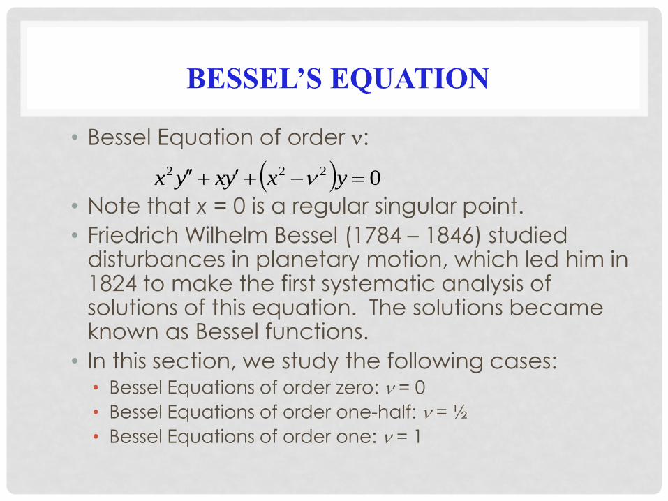
• Bessel Equation of order :

• Note that x = 0 is a regular singular point.

• Friedrich Wilhelm Bessel (1784 – 1846) studied disturbances in planetary motion, which led him in 1824 to make the first systematic analysis of solutions of this equation. The solutions became known as Bessel functions.

• In this section, we study the following cases: • Bessel Equations of order zero: = 0

• Bessel Equations of order one-half: = ½

• Bessel Equations of order one: = 1

0222 yxyxyx

BESSEL EQUATION OF ORDER ZERO

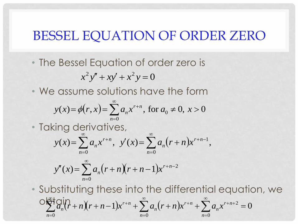
• The Bessel Equation of order zero is

• We assume solutions have the form

• Taking derivatives,

• Substituting these into the differential equation, we

obtain

0

2

0 0

1

1)(

,)(,)(

n

nr

n

n n

nr

n

nr

n

xnrnraxy

xnraxyxaxy

0,0for ,,)(0

0

n

nr

n xaxaxrxy

022 yxyxyx

010

2

00

n

nr

n

n

nr

n

n

nr

n xaxnraxnrnra

INDICIAL EQUATION

• From the previous slide,

• Rewriting,

• or

• The indicial equation is r2 = 0, and hence r1 = r2 = 0.

010

2

00

n

nr

n

n

nr

n

n

nr

n xaxnraxnrnra

01

)1()1()1(

2

2

1

10

nr

n

nn

rr

xanrnrnra

xrrraxrrra

0)1(2

2

212

1

2

0

nr

n

nn

rr xanraxraxra

RECURRENCE RELATION


• Note that a1 = 0; the recurrence relation is

• We conclude a1 = a3 = a5 = … = 0, and since r = 0,

• Note: Recall dependence of an on r, which is indicated by an(r). Thus we may write a2m(0) here instead of a2m.

,3,2,

2

2

nnr

aa n

n

0)1(2

2

212

1

2

0

nr

n

nn

rr xanraxraxra

,2,1,)2( 2

222 m

m

aa m

m

FIRST SOLUTION


• Thus

and in general,

• Thus

,2,1,)2( 2

222 m

m

aa m

m

,

1232,

122244,

226

0624

0

22

0

2

242

02

aa

aaaa

aa

,2,1,

!2

)1(22

02

m

m

aa

m

m

m

0,

!2

)1(1)(

122

2

01

xm

xaxy

mm

mm

BESSEL FUNCTION OF FIRST KIND ORDER ZERO

• Our first solution of Bessel’s Equation of order zero is

• The series converges for all x, and is called the Bessel function of the first kind of order zero, denoted by

• The graphs of J0 and several partial sum approximations are given here.

0,

!2

)1(1)(

122

2

01

xm

xaxy

mm

mm

0,

!2

)1()(

022

2

0

xm

xxJ

mm

mm

SECOND SOLUTION: ODD COEFFICIENTS

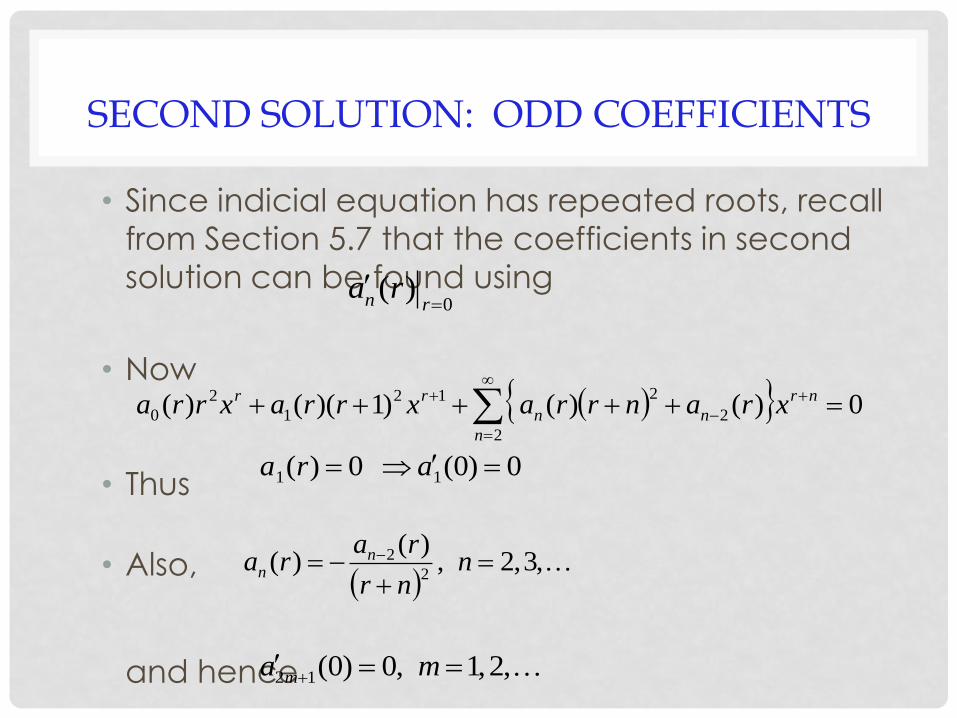
• Since indicial equation has repeated roots, recall

from Section 5.7 that the coefficients in second

solution can be found using

• Now

• Thus

• Also,

and hence

0)0(0)( 11 ara

0)()()1)(()(2

2

212

1

2

0

nr

n

nn

rr xranrraxrraxrra

,3,2,

)()(

2

2

nnr

rara n

n

0)(

rn ra

,2,1,0)0(12 ma m

SECOND SOLUTION: EVEN COEFFICIENTS

• Thus we need only compute derivatives of the

even coefficients, given by

• It can be shown that

and hence

1,

22

)1()(

2

)()(

22

022

222

m

mrr

ara

mr

rara

m

mm

m

mrrrra

ra

m

m

2

1

4

1

2

12

)(

)(

2

2

)0(2

1

4

1

2

12)0( 22 mm a

ma

SECOND SOLUTION: SERIES REPRESENTATION

• Thus

where

• Taking a0 = 1 and using results of Section 5.7,

,2,1,

!2

)1()0(

22

02

m

m

aHa

m

m

mm

mHm

2

1

4

1

2

1

0,

!2

)1(ln)()( 2

122

1

02

xxm

HxxJxy m

mm

m

m

BESSEL FUNCTION OF SECOND KIND, ORDER ZERO

• Instead of using y2, the second solution is often

taken to be a linear combination Y0 of J0 and y2,

known as the Bessel function of second kind of

order zero. Here, we take

• The constant is the Euler-Mascheroni constant,

defined by

• Substituting the expression for y2 from previous slide

into equation for Y0 above, we obtain

)(2ln)(2

)( 020 xJxyxY

5772.0lnlim

nHnn

0,

!2

)1()(

2ln

2)( 2

122

1

00

xxm

HxJ

xxY m

mm

m

m

GENERAL SOLUTION OF BESSEL’S EQUATION,

ORDER ZERO

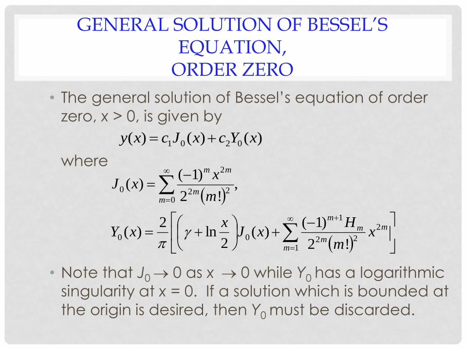
• The general solution of Bessel’s equation of order

zero, x > 0, is given by

where

• Note that J0 0 as x 0 while Y0 has a logarithmic

singularity at x = 0. If a solution which is bounded at

the origin is desired, then Y0 must be discarded.

m

mm

m

m

mm

mm

xm

HxJ

xxY

m

xxJ

2

122

1

00

022

2

0

!2

)1()(

2ln

2)(

,!2

)1()(

)()()( 0201 xYcxJcxy

GRAPHS OF BESSEL FUNCTIONS, ORDER ZERO

• The graphs of J0 and Y0 are given below.

• Note that the behavior of J0 and Y0 appear to be

similar to sin x and cos x for large x, except that

oscillations of J0 and Y0 decay to zero.

APPROXIMATION OF BESSEL FUNCTIONS, ORDER ZERO

• The fact that J0 and Y0 appear similar to sin x and

cos x for large x may not be surprising, since ODE

can be rewritten as

• Thus, for large x, our equation can be

approximated by

whose solns are sin x and cos x. Indeed, it can be

shown that

011

02

2222

y

x

vy

xyyvxyxyx

xxx

xY

xxx

xJ

as,4

sin2

)(

as,4

cos2

)(

2/1

0

2/1

0

,0 yy

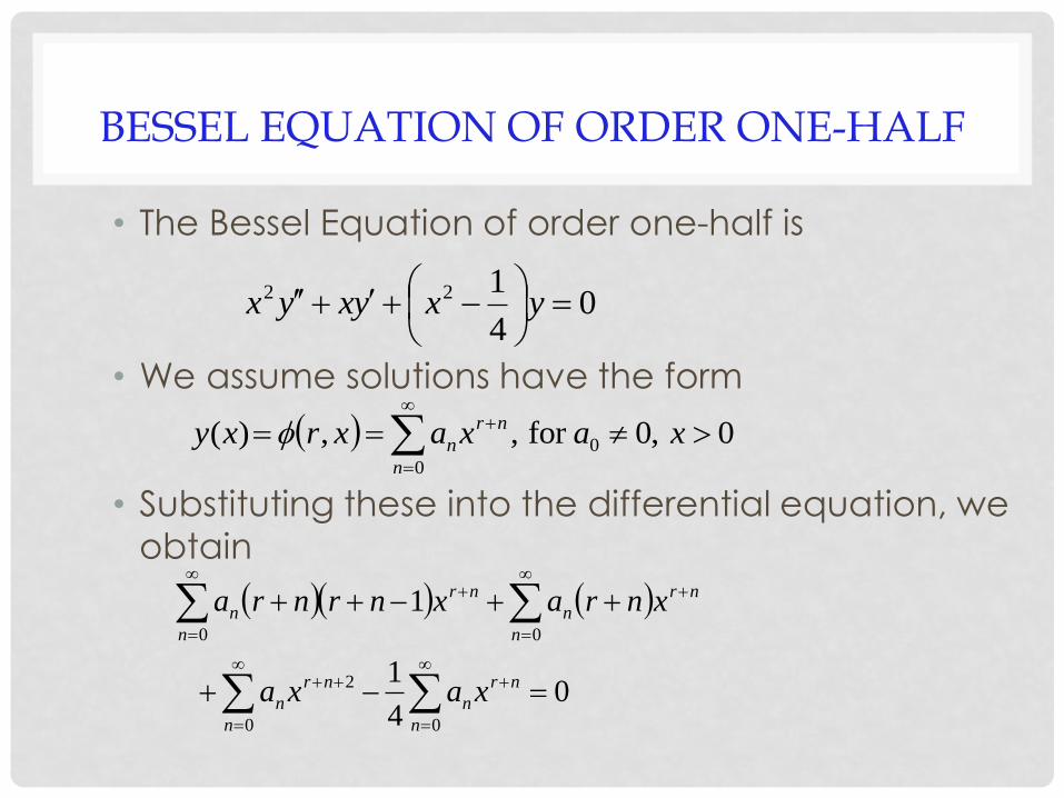
BESSEL EQUATION OF ORDER ONE-HALF

• The Bessel Equation of order one-half is



obtain

0,0for ,,)(0

0

n

nr

n xaxaxrxy

04

122

yxyxyx

04

1

1

00

2

00

n

nr

n

n

nr

n

n

nr

n

n

nr

n

xaxa

xnraxnrnra

RECURRENCE RELATION

• Using results of previous slide, we obtain

or

• The roots of indicial equation are r1 = ½, r2 = - ½ ,

and note that they differ by a positive integer.

• The recurrence relation is

04

1

4

1)1(

4

1

2

2

21

1

2

0

2

nr

n

nn

rr xaanrxarxar

04

11

0

2

0

n

nr

n

n

nr

n xaxanrnrnr

,3,2,

4/1

)()(

2

2

nnr

rara n

n

FIRST SOLUTION: COEFFICIENTS

• Consider first the case r1 = ½. From the previous slide,

• Since r1 = ½, a1 = 0, and hence from the recurrence relation, a1 = a3 = a5 = … = 0. For the even coefficients, we have

• It follows that

and

,2,1,

1224/122/1

22

2

222

m

mm

a

m

aa mm

m

,!545

,!3

024

02

aaa

aa

,2,1,!)12(

)1( 02

m

m

aa

m

m

04

1

4

1)1(4/1

2

2

21

1

2

0

2

nr

n

nn

rr xaanrxarxar

BESSEL FUNCTION OF FIRST KIND, ORDER ONE-HALF

• It follows that the first solution of our equation is, for

a0 = 1,

• The Bessel function of the first kind of order one-

half, J½, is defined as

0,sin

0,!)12(

)1(

0,!)12(

)1(1)(

2/1

0

122/1

1

22/1

1

xxx

xxm

x

xxm

xxy

m

mm

m

mm

0,sin2

)(2

)(

2/1

1

2/1

2/1

xx

xxyxJ

SECOND SOLUTION: EVEN COEFFICIENTS

• Now consider the case r2 = - ½. We know that

• Since r2 = - ½ , a1 = arbitrary. For the even

coefficients,

• It follows that

and

04

1

4

1)1(4/1

2

2

21

1

2

0

2

nr

n

nn

rr xaanrxarxar

,2,1,

1224/122/1

22

2

222

m

mm

a

m

aa mm

m

,!434

,!2

024

02

aaa

aa

,2,1,!)2(

)1( 02

m

m

aa

m

m

SECOND SOLUTION: ODD COEFFICIENTS

• For the odd coefficients,

• It follows that

and

,2,1,

1224/1122/1

12

2

1212

mmm

a

m

aa mm

m

,!545

,!3

13

5

1

3

aaa

aa

,2,1,!)12(

)1( 112

m

m

aa

m

m

SECOND SOLUTION

• Therefore

• The second solution is usually taken to be the function

where a0 = (2/)½ and a1 = 0.

• The general solution of Bessel’s equation of order one-half is

0,sincos

0,!)12(

)1(

!)2(

)1()(

10

2/1

0

12

1

0

2

0

2/1

2

xxaxax

xm

xa

m

xaxxy

m

mm

m

mm

0,cos2

)(

2/1

2/1

xx

xxJ

)()()( 2/122/11 xJcxJcxy

GRAPHS OF BESSEL FUNCTIONS, ORDER ONE-HALF

• Graphs of J½ , J-½ are given below. Note behavior of

J½ , J-½ similar to J0 , Y0 for large x, with phase shift of

/4.

xxx

xYxx

xJ

xx

xJxx

xJ

as,4

sin2

)(,4

cos2

)(

sin2

)(,cos2

)(

2/1

0

2/1

0

2/1

2/1

2/1

2/1

BESSEL EQUATION OF ORDER ONE

• The Bessel Equation of order one is



obtain

0,0for ,,)(0

0

n

nr

n xaxaxrxy

0122 yxyxyx

0

1

00

2

00

n

nr

n

n

nr

n

n

nr

n

n

nr

n

xaxa

xnraxnrnra

RECURRENCE RELATION

• Using the results of the previous slide, we obtain

or

• The roots of indicial equation are r1 = 1, r2 = - 1, and

note that they differ by a positive integer.

• The recurrence relation is

011)1(12

2

21

1

2

0

2

nr

n

nn

rr xaanrxarxar

0110

2

0

n

nr

n

n

nr

n xaxanrnrnr

,3,2,

1

)()(

2

2

nnr

rara n

n

FIRST SOLUTION: COEFFICIENTS

• Consider first the case r1 = 1. From previous slide,

• Since r1 = 1, a1 = 0, and hence from the

recurrence relation, a1 = a3 = a5 = … = 0. For the

even coefficients, we have

• It follows that

and

,2,1,

121212

22

2

222

m

mm

a

m

aa mm

m

,!2!32232

,122 4

0

2

242

02

aaa

aa

,2,1,!!)1(2

)1(2

02

m

mm

aa

m

m

m

011)1(12

2

21

1

2

0

2

nr

n

nn

rr xaanrxarxar

BESSEL FUNCTION OF FIRST KIND, ORDER ONE

• It follows that the first solution of our differential

equation is

• Taking a0 = ½, the Bessel function of the first kind of

order one, J1, is defined as

• The series converges for all x and hence J1 is

analytic everywhere.

0,!!)1(2

)1(1)(

1

2

201

xxmm

xaxym

m

m

m

0,!!)1(2

)1(

2)(

0

2

21

xxmm

xxJ

m

m

m

m

SECOND SOLUTION

• For the case r1 = -1, a solution of the form

is guaranteed by Theorem 5.7.1.

• The coefficients cn are determined by substituting y2 into the ODE and obtaining a recurrence relation, etc. The result is:

where Hk is as defined previously. See text for more details.

• Note that J1 0 as x 0 and is analytic at x = 0, while y2 is unbounded at x = 0 in the same manner as 1/x.

0,1ln)()( 2

1

1

12

xxcxxxJaxy n

n

n

0,

!)1(!2

)1(1ln)()( 2

12

11

12

xxmm

HHxxxJxy n

mm

mm

m

BESSEL FUNCTION OF SECOND KIND, ORDER ONE

• The second solution, the Bessel function of the second kind of order one, is usually taken to be the function

where is the Euler-Mascheroni constant.

• The general solution of Bessel’s equation of order one is

• Note that J1 , Y1 have same behavior at x = 0 as observed on previous slide for J1 and y2.

0,)(2ln)(2

)( 121 xxJxyxY

0),()()( 1211 xxYcxJcxy

2017- 2018 computational mathematics and … ppt_5.pdfcomputational mathematics and integral...

Documents