20150326.journal club
TRANSCRIPT

Journal(Club(�Jo�(Visualizing(Object(Detec6on(Features�
Vondrick,(C.(et(al.(In(Proc.(Interna6onal(Conference(on(
Computer(Vision(2013((
2015/03/26([email protected]�

Overview�
• f�³��ÎÐ×áUC(– a?F�(HOG,(SIFT,(etc)(– ��%((SVM,(Log.(regression,(etc)((
• “f�³°³C�ù�K¥�À�”(ÃG]¦À³´B+¯�¥�((
• HOG�a?��¾³!|�Ãv��

�²z�Àï�
Car�
HOG(+(SVM(®`�T�Ãv�¯�¡·�pS²±À�
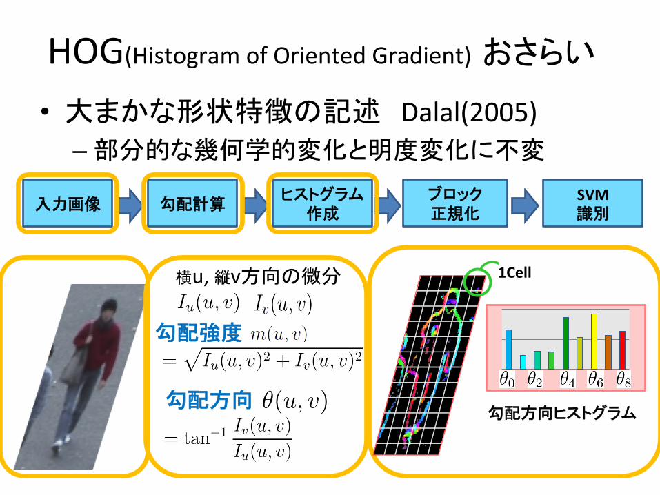
HOG(Histogram(of(Oriented(Gradient)��¤¾��
• -¸�±<ba?³���Dalal(2005)(– ��h±7�/h*�¯N9*�²�*�
��f�� ���n�ÞçÖÉ!X{��
SVM!���
ÛÐØÊäá C�
��L#ÛÐØÊäá�
1Cell�Vu,(rvL#³>��
��L#�
��;9�

��L#ÛÐØÊäá�
1Cell�
HOG(Histogram(of(Oriented(Gradient)�• -¸�±<ba?³���Dalal(2005)(– ��h±7�/h*�¯N9*�²�*�
��f�� ���n�ÞçÖÉ!X{��
SVM!���
ÛÐØÊäá C�
1Block!=!3Cell×3Cell�
V!:!Blocka?�!L2norm²½¿!X{��
Cell!,!Block²½¿7�/h*��N9*�²0@!

�²z�Àï�
Car�Car

�²z�Àï(via(HOG(glyph)�
Car

!|�E\:(Paired(Dict.Learning�Method: Paired Dictionary
+
=
= +...+
+...++
↵1 ↵2 ↵k
↵1 ↵2 ↵k
y = f(x) = V ↵
where ↵ = argmin↵
||x� U↵||22 s.t. ||↵||1 �
Method: Paired Dictionary
+
=
= +...+
+...++
↵1 ↵2 ↵k
↵1 ↵2 ↵k
y = f(x) = V ↵
where ↵ = argmin↵
||x� U↵||22 s.t. ||↵||1 �
Method: Paired Dictionary
+
=
= +...+
+...++
↵1 ↵2 ↵k
↵1 ↵2 ↵k
y = f(x) = V ↵
where ↵ = argmin↵
||x� U↵||22 s.t. ||↵||1 �
Method: Paired Dictionary
+
=
= +...+
+...++
↵1 ↵2 ↵k
↵1 ↵2 ↵k
y = f(x) = V ↵
where ↵ = argmin↵
||x� U↵||22 s.t. ||↵||1 �
= α1� + α2� + …+ αM�
u1� u2� uM�
x�
Method: Paired Dictionary
+
=
= +...+
+...++
↵1 ↵2 ↵k
↵1 ↵2 ↵k
y = f(x) = V ↵
where ↵ = argmin↵
||x� U↵||22 s.t. ||↵||1 �
Method: Paired Dictionary
+
=
= +...+
+...++
↵1 ↵2 ↵k
↵1 ↵2 ↵k
y = f(x) = V ↵
where ↵ = argmin↵
||x� U↵||22 s.t. ||↵||1 �
Method: Paired Dictionary
+
=
= +...+
+...++
↵1 ↵2 ↵k
↵1 ↵2 ↵k
y = f(x) = V ↵
where ↵ = argmin↵
||x� U↵||22 s.t. ||↵||1 �
Method: Paired Dictionary
+
=
= +...+
+...++
↵1 ↵2 ↵k
↵1 ↵2 ↵k
y = f(x) = V ↵
where ↵ = argmin↵
||x� U↵||22 s.t. ||↵||1 �
α1� + α2� + …+ αM� =�
v1� v2� vM�y�

)8�U, V(³/s�
• ih�I:(Paired(Dic6onary(Learning�

=¾ÁÀ)8àų��
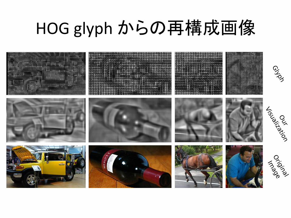
HOG(glyph(�¾³�UCf��
��
Figure 3: We visualize some high scoring detections from the deformable parts model [8] for person, chair, and car. Can youguess which are false alarms? Take a minute to study this figure, then see Figure 16 for the corresponding RGB patches.
Figure 4: In this paper, we present algorithms to visualizeHOG features. Our visualizations are perceptually intuitivefor humans to understand.
object detection features to natural images. Although we fo-cus on HOG features in this paper, our approach is generaland can be applied to other features as well. We evaluateour inversions with both automatic benchmarks and a largehuman study, and we found our visualizations are percep-tually more accurate at representing the content of a HOGfeature than existing methods; see Figure 4 for a compar-ison between our visualization and HOG glyphs. We thenuse our visualizations to inspect the behaviors of object de-tection systems and analyze their features. Since we hopeour visualizations will be useful to other researchers, ourfinal contribution is a public feature visualization toolbox.
2. Related WorkOur visualization algorithms extend an actively growing
body of work in feature inversion. Torralba and Oliva, inearly work, described a simple iterative procedure to re-cover images only given gist descriptors [17]. Weinzaepfelet al. [22] were the first to reconstruct an image given itskeypoint SIFT descriptors [13]. Their approach obtainscompelling reconstructions using a nearest neighbor basedapproach on a massive database. d’Angelo et al. [4] then de-veloped an algorithm to reconstruct images given only LBPfeatures [2, 1]. Their method analytically solves for the in-verse image and does not require a dataset.
While [22, 4, 17] do a good job at reconstructing im-ages from SIFT, LBP, and gist features, our visualizationalgorithms have several advantages. Firstly, while existingmethods are tailored for specific features, our visualizationalgorithms we propose are feature independent. Since wecast feature inversion as a machine learning problem, ouralgorithms can be used to visualize any feature. In this pa-per, we focus on features for object detection, the most pop-ular of which is HOG. Secondly, our algorithms are fast:our best algorithm can invert features in under a second ona desktop computer, enabling interactive visualization. Fi-nally, to our knowledge, this paper is the first to invert HOG.
Our visualizations enable analysis that complement a re-cent line of papers that provide tools to diagnose objectrecognition systems, which we briefly review here. Parikhand Zitnick [18, 19] introduced a new paradigm for humandebugging of object detectors, an idea that we adopt in ourexperiments. Hoiem et al. [10] performed a large study an-alyzing the errors that object detectors make. Divvala et al.[5] analyze part-based detectors to determine which com-ponents of object detection systems have the most impacton performance. Tatu et al. [20] explored the set of imagesthat generate identical HOG descriptors. Liu and Wang [12]designed algorithms to highlight which image regions con-tribute the most to a classifier’s confidence. Zhu et al. [24]try to determine whether we have reached Bayes risk forHOG. The tools in this paper enable an alternative mode toanalyze object detectors through visualizations. By puttingon ‘HOG glasses’ and visualizing the world according tothe features, we are able to gain a better understanding ofthe failures and behaviors of our object detection systems.
3. Feature Visualization Algorithms
We pose the feature visualization problem as one of fea-ture inversion, i.e. recovering the natural image that gen-erated a feature vector. Let x 2 RD be an image andy = �(x) be the corresponding HOG feature descriptor.Since �(·) is a many-to-one function, no analytic inverseexists. Hence, we seek an image x that, when we compute
2
HOG�³¹�À�g�Category ELDA Ridge Direct PairDictbicycle 0.452 0.577 0.513 0.561bottle 0.697 0.683 0.660 0.671car 0.668 0.677 0.652 0.639cat 0.749 0.712 0.687 0.705chair 0.660 0.621 0.604 0.617table 0.656 0.617 0.582 0.614motorbike 0.573 0.617 0.549 0.592person 0.696 0.667 0.646 0.646Mean 0.671 0.656 0.620 0.637
Table 1: We evaluate the performance of our inversion al-gorithm by comparing the inverse to the ground truth imageusing the mean normalized cross correlation. Higher is bet-ter; a score of 1 is perfect. See supplemental for full table.
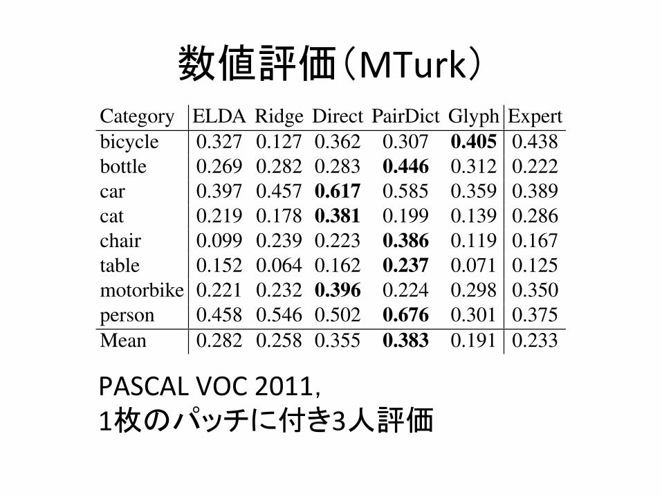
Category ELDA Ridge Direct PairDict Glyph Expertbicycle 0.327 0.127 0.362 0.307 0.405 0.438bottle 0.269 0.282 0.283 0.446 0.312 0.222car 0.397 0.457 0.617 0.585 0.359 0.389cat 0.219 0.178 0.381 0.199 0.139 0.286chair 0.099 0.239 0.223 0.386 0.119 0.167table 0.152 0.064 0.162 0.237 0.071 0.125motorbike 0.221 0.232 0.396 0.224 0.298 0.350person 0.458 0.546 0.502 0.676 0.301 0.375Mean 0.282 0.258 0.355 0.383 0.191 0.233
Table 2: We evaluate visualization performance acrosstwenty PASCAL VOC categories by asking MTurk work-ers to classify our inversions. Numbers are percent classi-fied correctly; higher is better. Chance is 0.05. Glyph refersto the standard black-and-white HOG diagram popularizedby [3]. Paired dictionary learning provides the best visu-alizations for humans. Expert refers to MIT PhD studentsin computer vision performing the same visualization chal-lenge with HOG glyphs. See supplemental for full table.
their answer. We also compared our algorithms against thestandard black-and-white HOG glyph popularized by [3].
Our results in Table 2 show that paired dictionary learn-ing and direct optimization provide the best visualizationof HOG descriptors for humans. Ridge regression and ex-emplar LDA performs better than the glyph, but they suf-fer from blurred inversions. Human performance on theHOG glyph is generally poor, and participants were eventhe slowest at completing that study. Interestingly, the glyphdoes the best job at visualizing bicycles, likely due to theirunique circular gradients. Our results overall suggest thatvisualizing HOG with the glyph is misleading, and richervisualizations from our paired dictionary are useful for in-terpreting HOG vectors.
Our experiments suggest that humans can predict theperformance of object detectors by only looking at HOGvisualizations. Human accuracy on inversions and state-of-the-art object detection AP scores from [7] are correlated
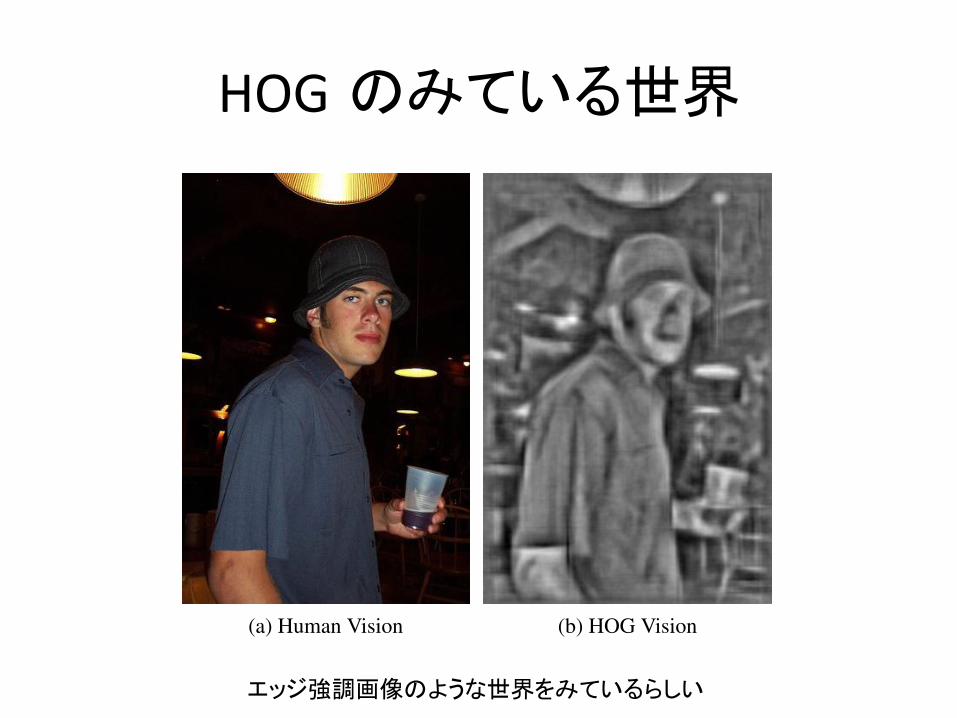
(a) Human Vision (b) HOG Vision
Figure 13: HOG inversion reveals the world that object de-tectors see. The left shows a man standing in a dark room.If we compute HOG on this image and invert it, the previ-ously dark scene behind the man emerges. Notice the wallstructure, the lamp post, and the chair in the bottom righthand corner.
with a Spearman’s rank correlation coefficient of 0.77.We also asked computer vision PhD students at MIT to
classify HOG glyphs in order to compare MTurk workerswith experts in HOG. Our results are summarized in thelast column of Table 2. HOG experts performed slightlybetter than non-experts on the glyph challenge, but expertson glyphs did not beat non-experts on other visualizations.This result suggests that our algorithms produce more intu-itive visualizations even for object detection researchers.
5. Understanding Object DetectorsWe have so far presented four algorithms to visualize ob-
ject detection features. We evaluated the visualizations witha large human study, and we found that paired dictionarylearning provides the most intuitive visualization of HOGfeatures. In this section, we will use this visualization toinspect the behavior of object detection systems.
5.1. HOG GogglesOur visualizations reveal that the world that features see
is slightly different from the world that the human eye per-ceives. Figure 13a shows a normal photograph of a manstanding in a dark room, but Figure 13b shows how HOGfeatures see the same man. Since HOG is invariant to illu-mination changes and amplifies gradients, the backgroundof the scene, normally invisible to the human eye, material-izes in our visualization.
In order to understand how this clutter affects object de-tection, we visualized the features of some of the top falsealarms from the Felzenszwalb et al. object detection sys-tem [8] when applied to the PASCAL VOC 2007 test set.
6
ÇÖÏ;�f�³½�±�gù�À¾¥��
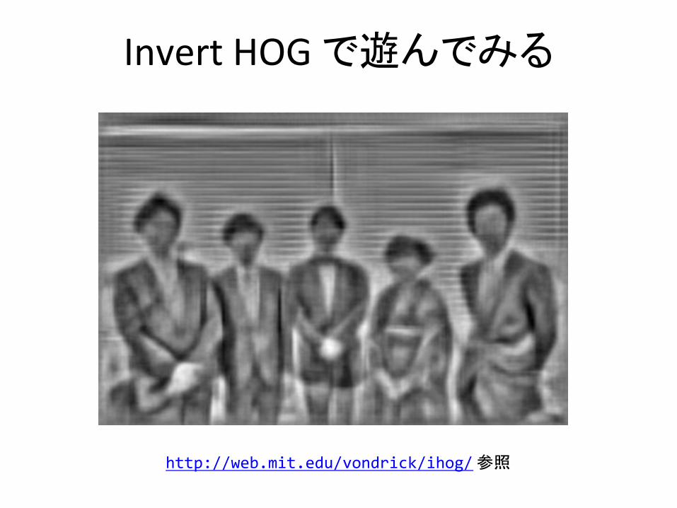
Invert(HOG(®�Ä®¹À�
http://web.mit.edu/vondrick/ihog/( _�
HOG(³ÒæÍÆѲAu´�.¦À�
Figure 9: We show results where our paired dictionary al-gorithm is trained to recover RGB images instead of onlygrayscale images. The right shows the original image andthe left shows the inverse.
PairDict (seconds) Greedy (days) OriginalFigure 10: Although our algorithms are good at invertingHOG, they are not perfect, and struggle to reconstruct highfrequency detail. See text for details.
Original xx
0 = �
�1 (�(x)) x
00 = �
�1 (�(x0))
Figure 11: We recursively compute HOG and invert it with apaired dictionary. While there is some information loss, ourvisualizations still do a good job at accurately representingHOG features. �(·) is HOG, and �
�1(·) is the inverse.
duce blurred visualizations. Direct optimization recovershigh frequency details at the expense of extra noise. Paireddictionary learning tends to produce the best visualizationfor HOG descriptors. By learning a dictionary over the vi-sual world and the correlation between HOG and naturalimages, paired dictionary learning recovered high frequen-cies without introducing significant noise.
We discovered that the paired dictionary is able to re-cover color from HOG descriptors. Figure 9 shows the re-sult of training a paired dictionary to estimate RGB imagesinstead of grayscale images. While the paired dictionaryassigns arbitrary colors to man-made objects and in-doorscenes, it frequently colors natural objects correctly, such asgrass or the sky, likely because those categories are stronglycorrelated to HOG descriptors. We focus on grayscale visu-alizations in this paper because we found those to be moreintuitive for humans to understand.
While our visualizations do a good job at representingHOG features, they have some limitations. Figure 10 com-pares our best visualization (paired dictionary) against agreedy algorithm that draws triangles of random rotation,
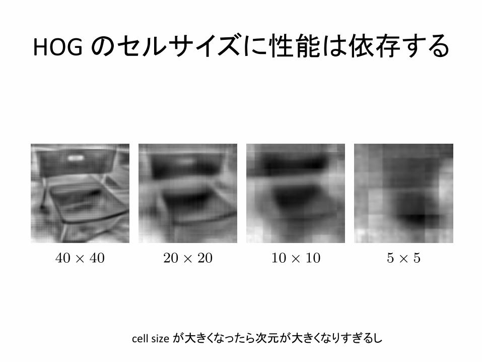
40⇥ 40 20⇥ 20 10⇥ 10 5⇥ 5
Figure 12: Our inversion algorithms are sensitive to theHOG template size. We show how performance degradesas the template becomes smaller.
scale, position, and intensity, and only accepts the triangleif it improves the reconstruction. If we allow the greedy al-gorithm to execute for an extremely long time (a few days),the visualization better shows higher frequency detail. Thisreveals that there exists a visualization better than paireddictionary learning, although it may not be tractable. In arelated experiment, Figure 11 recursively computes HOGon the inverse and inverts it again. This recursion showsthat there is some loss between iterations, although it is mi-nor and appears to discard high frequency details. More-over, Figure 12 indicates that our inversions are sensitive tothe dimensionality of the HOG template. Despite these lim-itations, our visualizations are, as we will now show, stillperceptually intuitive for humans to understand.
We quantitatively evaluate our algorithms under twobenchmarks. Firstly, we use an automatic inversion metricthat measures how well our inversions reconstruct originalimages. Secondly, we conducted a large visualization chal-lenge with human subjects on Amazon Mechanical Turk(MTurk), which is designed to determine how well peoplecan infer high level semantics from our visualizations.
4.1. Inversion BenchmarkWe consider the inversion performance of our algorithm:
given a HOG feature y, how well does our inverse �
�1(y)
reconstruct the original pixels x for each algorithm? SinceHOG is invariant up to a constant shift and scale, we scoreeach inversion against the original image with normalizedcross correlation. Our results are shown in Table 1. Overall,exemplar LDA does the best at pixel level reconstruction.
4.2. Visualization BenchmarkWhile the inversion benchmark evaluates how well the
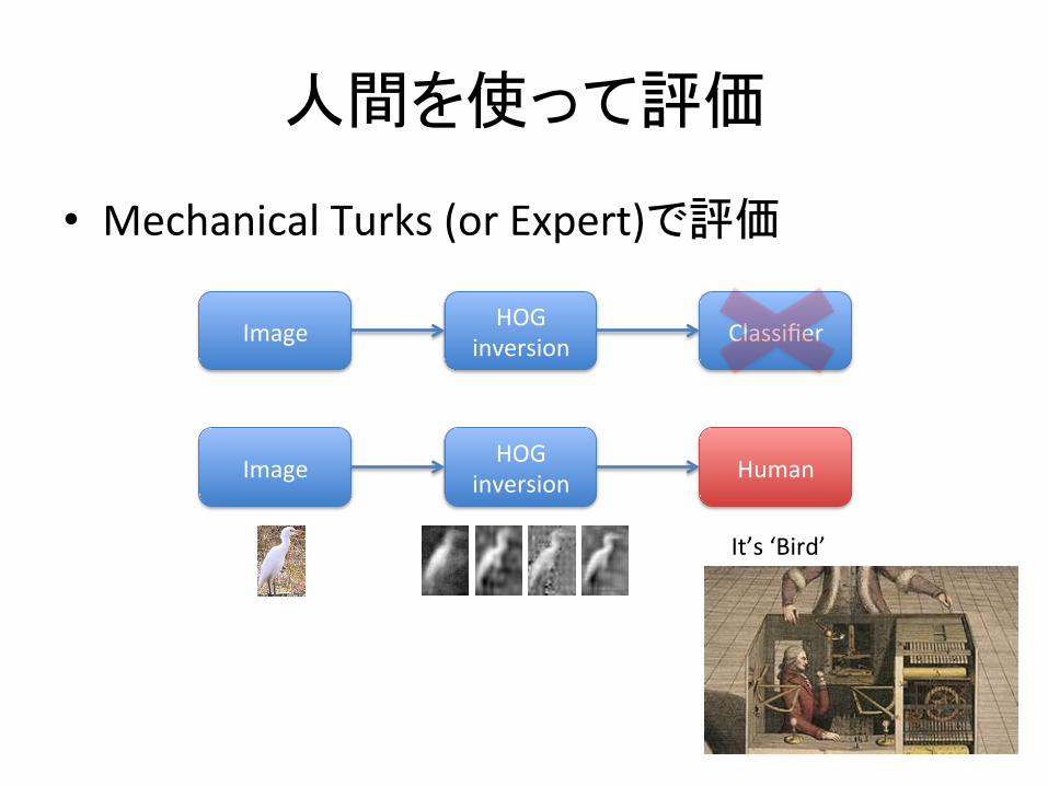
inversions reconstruct the original image, it does not cap-ture the high level content of the inverse: is the inverse of asheep still a sheep? To evaluate this, we conducted a studyon MTurk. We sampled 2,000 windows corresponding toobjects in PASCAL VOC 2011. We then showed partic-ipants an inversion from one of our algorithms and askedusers to classify it into one of the 20 categories. Each win-dow was shown to three different users. Users were requiredto pass a training course and qualification exam before par-ticipating in order to guarantee users understood the task.Users could optionally select that they were not confident in
5
cell(size(�-�¡±«©¾W��-�¡±¿¦ À¥�

E\¯³Z��
Figure 6: Inverting HOG using paired dictionary learning.We first project the HOG vector on to a HOG basis. Byjointly learning a coupled basis of HOG features and naturalimages, we then transfer the coefficients to the image basisto recover the natural image.
Figure 7: Some pairs of dictionaries for U and V . The leftof every pair is the gray scale dictionary element and theright is the positive components elements in the HOG dic-tionary. Notice the correlation between dictionaries.
Suppose we write x and y in terms of bases U 2 RD⇥K
and V 2 Rd⇥K respectively, but with shared coefficients↵ 2 RK :
x = U↵ and y = V ↵ (5)
The key observation is that inversion can be obtained byfirst projecting the HOG features y onto the HOG basis V ,then projecting ↵ into the natural image basis U :
�
�1D
(y) = U↵
⇤
where ↵
⇤= argmin
↵2RK
||V ↵� y||22 s.t. ||↵||1 �
(6)
See Figure 6 for a graphical representation of the paired dic-tionaries. Since efficient solvers for Eqn.6 exist [14, 11], wecan invert features in under two seconds on a 4 core CPU.
Paired dictionaries require finding appropriate bases U
and V such that Eqn.5 holds. To do this, we solve a paireddictionary learning problem, inspired by recent super reso-lution sparse coding work [23, 21]:
argmin
U,V,↵
NX
i=1
�||x
i
� U↵
i
||22 + ||�(xi
)� V ↵
i
||22�
s.t. ||↵i
||1 � 8i, ||U ||22 �1, ||V ||22 �2
(7)
After a few algebraic manipulations, the above objectivesimplifies to a standard sparse coding and dictionary learn-
Original ELDA Ridge Direct PairDict
Figure 8: We show results for all four of our inversion al-gorithms on held out image patches on similar dimensionscommon for object detection. See supplemental for more.
ing problem with concatenated dictionaries, which we op-timize using SPAMS [14]. Optimization typically took afew hours on medium sized problems. We estimate U andV with a dictionary size K ⇡ 10
3 and training samplesN ⇡ 10
6 from a large database. See Figure 7 for a visual-ization of the learned dictionary pairs.
4. Evaluation of VisualizationsWe evaluate our inversion algorithms using both quali-
tative and quantitative measures. We use PASCAL VOC2011 [6] as our dataset and we invert patches correspondingto objects. Any algorithm that required training could onlyaccess the training set. During evaluation, only images fromthe validation set are examined. The database for exemplarLDA excluded the category of the patch we were invertingto reduce the potential effect of dataset biases.
We show our inversions in Figure 8 for a few object cat-egories. Exemplar LDA and ridge regression tend to pro-
4

E\¯³Z�²¬�³x� (�
• ELDA(q<��%®ÐËÅåéÊ¥îØÖßK�³6'((�J�³:´î2¥*±[�¦À)(
• Ridge(f�(X(¯HOG(glyph(Y(³"O�4Ã(Ridge(&5®~¡(
• Direct(Gabor(äÆɱa?�U(®�~¥©�IÃP��(
• PairedDict.(QE\(

I���ìj��Ií�
Category ELDA Ridge Direct PairDictbicycle 0.452 0.577 0.513 0.561bottle 0.697 0.683 0.660 0.671car 0.668 0.677 0.652 0.639cat 0.749 0.712 0.687 0.705chair 0.660 0.621 0.604 0.617table 0.656 0.617 0.582 0.614motorbike 0.573 0.617 0.549 0.592person 0.696 0.667 0.646 0.646Mean 0.671 0.656 0.620 0.637
Table 1: We evaluate the performance of our inversion al-gorithm by comparing the inverse to the ground truth imageusing the mean normalized cross correlation. Higher is bet-ter; a score of 1 is perfect. See supplemental for full table.
Category ELDA Ridge Direct PairDict Glyph Expertbicycle 0.327 0.127 0.362 0.307 0.405 0.438bottle 0.269 0.282 0.283 0.446 0.312 0.222car 0.397 0.457 0.617 0.585 0.359 0.389cat 0.219 0.178 0.381 0.199 0.139 0.286chair 0.099 0.239 0.223 0.386 0.119 0.167table 0.152 0.064 0.162 0.237 0.071 0.125motorbike 0.221 0.232 0.396 0.224 0.298 0.350person 0.458 0.546 0.502 0.676 0.301 0.375Mean 0.282 0.258 0.355 0.383 0.191 0.233
Table 2: We evaluate visualization performance acrosstwenty PASCAL VOC categories by asking MTurk work-ers to classify our inversions. Numbers are percent classi-fied correctly; higher is better. Chance is 0.05. Glyph refersto the standard black-and-white HOG diagram popularizedby [3]. Paired dictionary learning provides the best visu-alizations for humans. Expert refers to MIT PhD studentsin computer vision performing the same visualization chal-lenge with HOG glyphs. See supplemental for full table.
their answer. We also compared our algorithms against thestandard black-and-white HOG glyph popularized by [3].
Our results in Table 2 show that paired dictionary learn-ing and direct optimization provide the best visualizationof HOG descriptors for humans. Ridge regression and ex-emplar LDA performs better than the glyph, but they suf-fer from blurred inversions. Human performance on theHOG glyph is generally poor, and participants were eventhe slowest at completing that study. Interestingly, the glyphdoes the best job at visualizing bicycles, likely due to theirunique circular gradients. Our results overall suggest thatvisualizing HOG with the glyph is misleading, and richervisualizations from our paired dictionary are useful for in-terpreting HOG vectors.
Our experiments suggest that humans can predict theperformance of object detectors by only looking at HOGvisualizations. Human accuracy on inversions and state-of-the-art object detection AP scores from [7] are correlated
(a) Human Vision (b) HOG Vision
Figure 13: HOG inversion reveals the world that object de-tectors see. The left shows a man standing in a dark room.If we compute HOG on this image and invert it, the previ-ously dark scene behind the man emerges. Notice the wallstructure, the lamp post, and the chair in the bottom righthand corner.
with a Spearman’s rank correlation coefficient of 0.77.We also asked computer vision PhD students at MIT to
classify HOG glyphs in order to compare MTurk workerswith experts in HOG. Our results are summarized in thelast column of Table 2. HOG experts performed slightlybetter than non-experts on the glyph challenge, but expertson glyphs did not beat non-experts on other visualizations.This result suggests that our algorithms produce more intu-itive visualizations even for object detection researchers.
5. Understanding Object DetectorsWe have so far presented four algorithms to visualize ob-
ject detection features. We evaluated the visualizations witha large human study, and we found that paired dictionarylearning provides the most intuitive visualization of HOGfeatures. In this section, we will use this visualization toinspect the behavior of object detection systems.
5.1. HOG GogglesOur visualizations reveal that the world that features see
is slightly different from the world that the human eye per-ceives. Figure 13a shows a normal photograph of a manstanding in a dark room, but Figure 13b shows how HOGfeatures see the same man. Since HOG is invariant to illu-mination changes and amplifies gradients, the backgroundof the scene, normally invisible to the human eye, material-izes in our visualization.
In order to understand how this clutter affects object de-tection, we visualized the features of some of the top falsealarms from the Felzenszwalb et al. object detection sys-tem [8] when applied to the PASCAL VOC 2007 test set.
6
�¸¿½Â¥¡±�(´êωêð)�
PASCAL(VOC(2011î8(ÉäÐÃe�©����
��Ã�«���
• Mechanical(Turks((or(Expert)®���
Image� HOG(inversion� Classifier�
Image� HOG(inversion� Human�
Figure 6: Inverting HOG using paired dictionary learning.We first project the HOG vector on to a HOG basis. Byjointly learning a coupled basis of HOG features and naturalimages, we then transfer the coefficients to the image basisto recover the natural image.
Figure 7: Some pairs of dictionaries for U and V . The leftof every pair is the gray scale dictionary element and theright is the positive components elements in the HOG dic-tionary. Notice the correlation between dictionaries.
Suppose we write x and y in terms of bases U 2 RD⇥K
and V 2 Rd⇥K respectively, but with shared coefficients↵ 2 RK :
x = U↵ and y = V ↵ (5)
The key observation is that inversion can be obtained byfirst projecting the HOG features y onto the HOG basis V ,then projecting ↵ into the natural image basis U :
�
�1D
(y) = U↵
⇤
where ↵
⇤= argmin
↵2RK
||V ↵� y||22 s.t. ||↵||1 �
(6)
See Figure 6 for a graphical representation of the paired dic-tionaries. Since efficient solvers for Eqn.6 exist [14, 11], wecan invert features in under two seconds on a 4 core CPU.
Paired dictionaries require finding appropriate bases U
and V such that Eqn.5 holds. To do this, we solve a paireddictionary learning problem, inspired by recent super reso-lution sparse coding work [23, 21]:
argmin
U,V,↵
NX
i=1
�||x
i
� U↵
i
||22 + ||�(xi
)� V ↵
i
||22�
s.t. ||↵i
||1 � 8i, ||U ||22 �1, ||V ||22 �2
(7)
After a few algebraic manipulations, the above objectivesimplifies to a standard sparse coding and dictionary learn-
Original ELDA Ridge Direct PairDict
Figure 8: We show results for all four of our inversion al-gorithms on held out image patches on similar dimensionscommon for object detection. See supplemental for more.
ing problem with concatenated dictionaries, which we op-timize using SPAMS [14]. Optimization typically took afew hours on medium sized problems. We estimate U andV with a dictionary size K ⇡ 10
3 and training samplesN ⇡ 10
6 from a large database. See Figure 7 for a visual-ization of the learned dictionary pairs.
4. Evaluation of VisualizationsWe evaluate our inversion algorithms using both quali-
tative and quantitative measures. We use PASCAL VOC2011 [6] as our dataset and we invert patches correspondingto objects. Any algorithm that required training could onlyaccess the training set. During evaluation, only images fromthe validation set are examined. The database for exemplarLDA excluded the category of the patch we were invertingto reduce the potential effect of dataset biases.
We show our inversions in Figure 8 for a few object cat-egories. Exemplar LDA and ridge regression tend to pro-
4
It’s(‘Bird’�
Common Missed Detections
Common False Alarms
The HOGgles Challenge
Common Missed Detections
Common False Alarms
The HOGgles Challenge
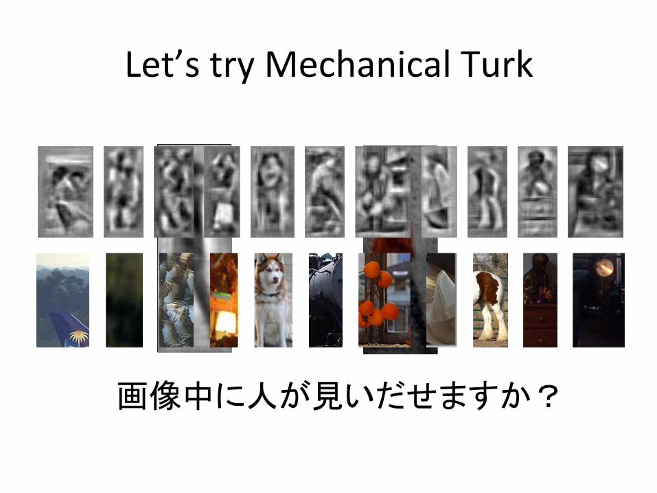
Let’s(try(Mechanical(Turk�
Figure 3: We visualize some high scoring detections from the deformable parts model [8] for person, chair, and car. Can youguess which are false alarms? Take a minute to study this figure, then see Figure 16 for the corresponding RGB patches.
Figure 4: In this paper, we present algorithms to visualizeHOG features. Our visualizations are perceptually intuitivefor humans to understand.
object detection features to natural images. Although we fo-cus on HOG features in this paper, our approach is generaland can be applied to other features as well. We evaluateour inversions with both automatic benchmarks and a largehuman study, and we found our visualizations are percep-tually more accurate at representing the content of a HOGfeature than existing methods; see Figure 4 for a compar-ison between our visualization and HOG glyphs. We thenuse our visualizations to inspect the behaviors of object de-tection systems and analyze their features. Since we hopeour visualizations will be useful to other researchers, ourfinal contribution is a public feature visualization toolbox.
2. Related WorkOur visualization algorithms extend an actively growing
body of work in feature inversion. Torralba and Oliva, inearly work, described a simple iterative procedure to re-cover images only given gist descriptors [17]. Weinzaepfelet al. [22] were the first to reconstruct an image given itskeypoint SIFT descriptors [13]. Their approach obtainscompelling reconstructions using a nearest neighbor basedapproach on a massive database. d’Angelo et al. [4] then de-veloped an algorithm to reconstruct images given only LBPfeatures [2, 1]. Their method analytically solves for the in-verse image and does not require a dataset.
While [22, 4, 17] do a good job at reconstructing im-ages from SIFT, LBP, and gist features, our visualizationalgorithms have several advantages. Firstly, while existingmethods are tailored for specific features, our visualizationalgorithms we propose are feature independent. Since wecast feature inversion as a machine learning problem, ouralgorithms can be used to visualize any feature. In this pa-per, we focus on features for object detection, the most pop-ular of which is HOG. Secondly, our algorithms are fast:our best algorithm can invert features in under a second ona desktop computer, enabling interactive visualization. Fi-nally, to our knowledge, this paper is the first to invert HOG.
Our visualizations enable analysis that complement a re-cent line of papers that provide tools to diagnose objectrecognition systems, which we briefly review here. Parikhand Zitnick [18, 19] introduced a new paradigm for humandebugging of object detectors, an idea that we adopt in ourexperiments. Hoiem et al. [10] performed a large study an-alyzing the errors that object detectors make. Divvala et al.[5] analyze part-based detectors to determine which com-ponents of object detection systems have the most impacton performance. Tatu et al. [20] explored the set of imagesthat generate identical HOG descriptors. Liu and Wang [12]designed algorithms to highlight which image regions con-tribute the most to a classifier’s confidence. Zhu et al. [24]try to determine whether we have reached Bayes risk forHOG. The tools in this paper enable an alternative mode toanalyze object detectors through visualizations. By puttingon ‘HOG glasses’ and visualizing the world according tothe features, we are able to gain a better understanding ofthe failures and behaviors of our object detection systems.
3. Feature Visualization Algorithms
We pose the feature visualization problem as one of fea-ture inversion, i.e. recovering the natural image that gen-erated a feature vector. Let x 2 RD be an image andy = �(x) be the corresponding HOG feature descriptor.Since �(·) is a many-to-one function, no analytic inverseexists. Hence, we seek an image x that, when we compute
2
Figure 15: We visualize a few deformable parts models trained with [8]. Notice the structure that emerges with our visual-ization. First row: car, person, bottle, bicycle, motorbike, potted plant. Second row: train, bus, horse, television, chair. Forthe right most visualizations, we also included the HOG glyph. Our visualizations tend to reveal more detail than the glyph.
Figure 16: We show the original RGB patches that correspond to the visualizations from Figure 3. We print the originalpatches on a separate page to highlight how the inverses of false positives look like true positives. We recommend comparingthis figure side-by-side with Figure 3.
paper includes HOG visualizations, we hope more intuitivevisualizations will prove useful for the community.
Acknowledgments: We thank Hamed Pirsiavash, Joseph Lim, MITCSAIL Vision Group, and reviewers. Funding was provided by a NSFGRFP to CV, a Facebook fellowship to AK, and a Google research award,ONR MURI N000141010933 and NSF Career Award No. 0747120 to AT.
References[1] A. Alahi, R. Ortiz, and P. Vandergheynst. Freak: Fast retina keypoint.
In CVPR, 2012. 2[2] M. Calonder, V. Lepetit, C. Strecha, and P. Fua. Brief: Binary robust
independent elementary features. ECCV, 2010. 2[3] N. Dalal and B. Triggs. Histograms of oriented gradients for human
detection. In CVPR, 2005. 6[4] E. d’Angelo, A. Alahi, and P. Vandergheynst. Beyond bits: Recon-
structing images from local binary descriptors. ICPR, 2012. 2[5] S. Divvala, A. Efros, and M. Hebert. How important are deformable
parts in the deformable parts model? Technical Report, 2012. 2[6] M. Everingham, L. Van Gool, C. K. I. Williams, J. Winn, and A. Zis-
serman. The pascal visual object classes challenge. IJCV, 2010. 4[7] P. Felzenszwalb, R. Girshick, and D. McAllester. Cascade object
detection with deformable part models. In CVPR, 2010. 6[8] P. Felzenszwalb, R. Girshick, D. McAllester, and D. Ramanan. Ob-
ject detection with discriminatively trained part-based models. PAMI,2010. 1, 2, 6, 7, 8
[9] B. Hariharan, J. Malik, and D. Ramanan. Discriminative decorrela-tion for clustering and classification. ECCV, 2012. 3
[10] D. Hoiem, Y. Chodpathumwan, and Q. Dai. Diagnosing error inobject detectors. ECCV, 2012. 2
[11] H. Lee, A. Battle, R. Raina, and A. Ng. Efficient sparse coding algo-rithms. NIPS, 2007. 4
[12] L. Liu and L. Wang. What has my classifier learned? visualizing theclassification rules of bag-of-feature model by support region detec-tion. In CVPR, 2012. 2
[13] D. Lowe. Object recognition from local scale-invariant features. InICCV, 1999. 2
[14] J. Mairal, F. Bach, J. Ponce, and G. Sapiro. Online dictionary learn-ing for sparse coding. In ICML, 2009. 4
[15] T. Malisiewicz, A. Gupta, and A. Efros. Ensemble of exemplar-svmsfor object detection and beyond. In ICCV, 2011. 3
[16] S. Nishimoto, A. Vu, T. Naselaris, Y. Benjamini, B. Yu, and J. Gal-lant. Reconstructing visual experiences from brain activity evokedby natural movies. Current Biology, 2011. 3
[17] A. Oliva and A. Torralba. Modeling the shape of the scene: A holisticrepresentation of the spatial envelope. IJCV, 2001. 2
[18] D. Parikh and C. Zitnick. Human-debugging of machines. In NIPSWCSSWC, 2011. 2, 7
[19] D. Parikh and C. L. Zitnick. The role of features, algorithms and datain visual recognition. In CVPR, 2010. 2, 7
[20] A. Tatu, F. Lauze, M. Nielsen, and B. Kimia. Exploring the repre-sentation capabilities of hog descriptors. In ICCV WIT, 2011. 2
[21] S. Wang, L. Zhang, Y. Liang, and Q. Pan. Semi-coupled dictio-nary learning with applications to image super-resolution and photo-sketch synthesis. In CVPR, 2012. 4
[22] P. Weinzaepfel, H. Jegou, and P. Perez. Reconstructing an imagefrom its local descriptors. In CVPR, 2011. 2
[23] J. Yang, J. Wright, T. Huang, and Y. Ma. Image super-resolution viasparse representation. Transactions on Image Processing, 2010. 4
[24] X. Zhu, C. Vondrick, D. Ramanan, and C. Fowlkes. Do we needmore training data or better models for object detection? BMVC,2012. 2
8
f��²��z�ª¨¸¦�ï�
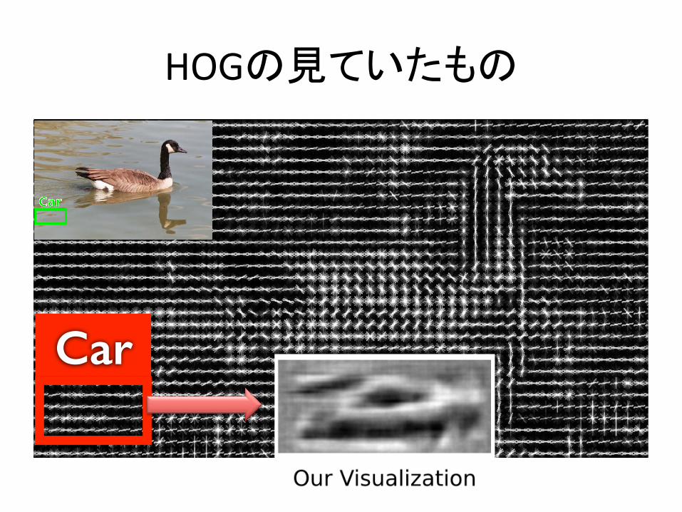
HOG³z�©»³�
Car
HOGgles: Visualizing Object Detection Features⇤
Carl Vondrick, Aditya Khosla, Tomasz Malisiewicz, Antonio TorralbaMassachusetts Institute of Technology
{vondrick,khosla,tomasz,torralba}@csail.mit.edu
Abstract
We introduce algorithms to visualize feature spaces usedby object detectors. The tools in this paper allow a humanto put on ‘HOG goggles’ and perceive the visual world asa HOG based object detector sees it. We found that thesevisualizations allow us to analyze object detection systemsin new ways and gain new insight into the detector’s fail-ures. For example, when we visualize the features for highscoring false alarms, we discovered that, although they areclearly wrong in image space, they do look deceptively sim-ilar to true positives in feature space. This result suggeststhat many of these false alarms are caused by our choice offeature space, and indicates that creating a better learningalgorithm or building bigger datasets is unlikely to correctthese errors. By visualizing feature spaces, we can gain amore intuitive understanding of our detection systems.
1. IntroductionFigure 1 shows a high scoring detection from an ob-
ject detector with HOG features and a linear SVM classifiertrained on PASCAL. Despite our field’s incredible progressin object recognition over the last decade, why do our de-tectors still think that sea water looks like a car?
Unfortunately, computer vision researchers are often un-able to explain the failures of object detection systems.Some researchers blame the features, others the training set,and even more the learning algorithm. Yet, if we wish tobuild the next generation of object detectors, it seems cru-cial to understand the failures of our current detectors.
In this paper, we introduce a tool to explain some of thefailures of object detection systems.1 We present algorithmsto visualize the feature spaces of object detectors. Sincefeatures are too high dimensional for humans to directly in-spect, our visualization algorithms work by inverting fea-tures back to natural images. We found that these inversionsprovide an intuitive and accurate visualization of the featurespaces used by object detectors.
⇤Previously: Inverting and Visualizing Features for Object Detection1Code is available online at http://mit.edu/vondrick/ihog
Figure 1: An image from PASCAL and a high scoring cardetection from DPM [8]. Why did the detector fail?
Figure 2: We show the crop for the false car detection fromFigure 1. On the right, we show our visualization of theHOG features for the same patch. Our visualization revealsthat this false alarm actually looks like a car in HOG space.
Figure 2 shows the output from our visualization on thefeatures for the false car detection. This visualization re-veals that, while there are clearly no cars in the originalimage, there is a car hiding in the HOG descriptor. HOGfeatures see a slightly different visual world than what wesee, and by visualizing this space, we can gain a more intu-itive understanding of our object detectors.
Figure 3 inverts more top detections on PASCAL fora few categories. Can you guess which are false alarms?Take a minute to study the figure since the next sentencemight ruin the surprise. Although every visualization lookslike a true positive, all of these detections are actually falsealarms. Consequently, even with a better learning algorithmor more data, these false alarms will likely persist. In otherwords, the features are to blame.
The principle contribution of this paper is the presenta-tion of algorithms for visualizing features used in object de-tection. To this end, we present four algorithms to invert
1
I���ìMTurkí�
PASCAL(VOC(2011î(1R³ÚÖÕ²�3����
Category ELDA Ridge Direct PairDictbicycle 0.452 0.577 0.513 0.561bottle 0.697 0.683 0.660 0.671car 0.668 0.677 0.652 0.639cat 0.749 0.712 0.687 0.705chair 0.660 0.621 0.604 0.617table 0.656 0.617 0.582 0.614motorbike 0.573 0.617 0.549 0.592person 0.696 0.667 0.646 0.646Mean 0.671 0.656 0.620 0.637
Table 1: We evaluate the performance of our inversion al-gorithm by comparing the inverse to the ground truth imageusing the mean normalized cross correlation. Higher is bet-ter; a score of 1 is perfect. See supplemental for full table.
Category ELDA Ridge Direct PairDict Glyph Expertbicycle 0.327 0.127 0.362 0.307 0.405 0.438bottle 0.269 0.282 0.283 0.446 0.312 0.222car 0.397 0.457 0.617 0.585 0.359 0.389cat 0.219 0.178 0.381 0.199 0.139 0.286chair 0.099 0.239 0.223 0.386 0.119 0.167table 0.152 0.064 0.162 0.237 0.071 0.125motorbike 0.221 0.232 0.396 0.224 0.298 0.350person 0.458 0.546 0.502 0.676 0.301 0.375Mean 0.282 0.258 0.355 0.383 0.191 0.233
Table 2: We evaluate visualization performance acrosstwenty PASCAL VOC categories by asking MTurk work-ers to classify our inversions. Numbers are percent classi-fied correctly; higher is better. Chance is 0.05. Glyph refersto the standard black-and-white HOG diagram popularizedby [3]. Paired dictionary learning provides the best visu-alizations for humans. Expert refers to MIT PhD studentsin computer vision performing the same visualization chal-lenge with HOG glyphs. See supplemental for full table.
their answer. We also compared our algorithms against thestandard black-and-white HOG glyph popularized by [3].
Our results in Table 2 show that paired dictionary learn-ing and direct optimization provide the best visualizationof HOG descriptors for humans. Ridge regression and ex-emplar LDA performs better than the glyph, but they suf-fer from blurred inversions. Human performance on theHOG glyph is generally poor, and participants were eventhe slowest at completing that study. Interestingly, the glyphdoes the best job at visualizing bicycles, likely due to theirunique circular gradients. Our results overall suggest thatvisualizing HOG with the glyph is misleading, and richervisualizations from our paired dictionary are useful for in-terpreting HOG vectors.
Our experiments suggest that humans can predict theperformance of object detectors by only looking at HOGvisualizations. Human accuracy on inversions and state-of-the-art object detection AP scores from [7] are correlated
(a) Human Vision (b) HOG Vision
Figure 13: HOG inversion reveals the world that object de-tectors see. The left shows a man standing in a dark room.If we compute HOG on this image and invert it, the previ-ously dark scene behind the man emerges. Notice the wallstructure, the lamp post, and the chair in the bottom righthand corner.
with a Spearman’s rank correlation coefficient of 0.77.We also asked computer vision PhD students at MIT to
classify HOG glyphs in order to compare MTurk workerswith experts in HOG. Our results are summarized in thelast column of Table 2. HOG experts performed slightlybetter than non-experts on the glyph challenge, but expertson glyphs did not beat non-experts on other visualizations.This result suggests that our algorithms produce more intu-itive visualizations even for object detection researchers.
5. Understanding Object DetectorsWe have so far presented four algorithms to visualize ob-
ject detection features. We evaluated the visualizations witha large human study, and we found that paired dictionarylearning provides the most intuitive visualization of HOGfeatures. In this section, we will use this visualization toinspect the behavior of object detection systems.
5.1. HOG GogglesOur visualizations reveal that the world that features see
is slightly different from the world that the human eye per-ceives. Figure 13a shows a normal photograph of a manstanding in a dark room, but Figure 13b shows how HOGfeatures see the same man. Since HOG is invariant to illu-mination changes and amplifies gradients, the backgroundof the scene, normally invisible to the human eye, material-izes in our visualization.
In order to understand how this clutter affects object de-tection, we visualized the features of some of the top falsealarms from the Felzenszwalb et al. object detection sys-tem [8] when applied to the PASCAL VOC 2007 test set.
6
a?�î��%³d~�
Figure 3 shows our visualizations of the features of the topfalse alarms. Notice how the false alarms look very simi-lar to true positives. While there are many different typesof detector errors, this result suggests that these particularfailures are due to limitations of HOG, and consequently,even if we develop better learning algorithms or use largerdatasets, these will false alarms will likely persist.
Figure 16 shows the corresponding RGB image patchesfor the false positives discussed above. Notice how whenwe view these detections in image space, all of the falsealarms are difficult to explain. Why do chair detectors fireon buses, or people detectors on cherries? By visualizingthe detections in feature space, we discovered that the learn-ing algorithm made reasonable failures since the featuresare deceptively similar to true positives.
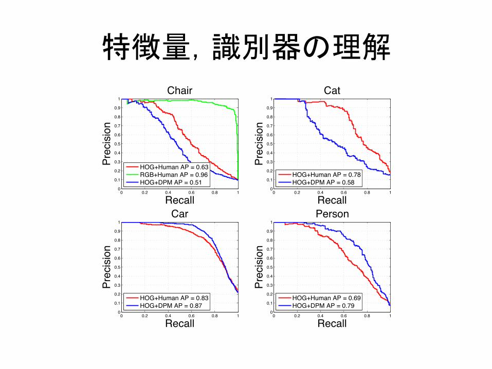
5.2. Human+HOG DetectorsAlthough HOG features are designed for machines, how
well do humans see in HOG space? If we could quantify hu-man vision on the HOG feature space, we could get insightsinto the performance of HOG with a perfect learning algo-rithm (people). Inspired by Parikh and Zitnick’s methodol-ogy [18, 19], we conducted a large human study where wehad Amazon Mechanical Turk workers act as sliding win-dow HOG based object detectors.
We built an online interface for humans to look at HOGvisualizations of window patches at the same resolution asDPM. We instructed workers to either classify a HOG vi-sualization as a positive example or a negative example fora category. By averaging over multiple people (we used 25people per window), we obtain a real value score for a HOGpatch. To build our dataset, we sampled top detections fromDPM on the PASCAL VOC 2007 dataset for a few cate-gories. Our dataset consisted of around 5, 000 windows percategory and around 20% were true positives.
Figure 14 shows precision recall curves for the Hu-man+HOG based object detector. In most cases, humansubjects classifying HOG visualizations were able to ranksliding windows with either the same accuracy or betterthan DPM. Humans tied DPM for recognizing cars, sug-gesting that performance may be saturated for car detectionon HOG. Humans were slightly superior to DPM for chairs,although performance might be nearing saturation soon.There appears to be the most potential for improvement fordetecting cats with HOG. Subjects performed slightly worstthan DPM for detecting people, but we believe this is thecase because humans tend to be good at fabricating peoplein abstract drawings.
We then repeated the same experiment as above on chairsexcept we instructed users to classify the original RGBpatch instead of the HOG visualization. As expected, hu-mans achieved near perfect accuracy at detecting chairswith RGB sliding windows. The performance gap be-
0 0.2 0.4 0.6 0.8 10
0.1
0.2
0.3
0.4
0.5
0.6
0.7
0.8
0.9
1
Recall
Prec
ision
Chair
HOG+Human AP = 0.63RGB+Human AP = 0.96HOG+DPM AP = 0.51
0 0.2 0.4 0.6 0.8 10
0.1
0.2
0.3
0.4
0.5
0.6
0.7
0.8
0.9
1
Recall
Prec
ision
Cat
HOG+Human AP = 0.78HOG+DPM AP = 0.58
0 0.2 0.4 0.6 0.8 10
0.1
0.2
0.3
0.4
0.5
0.6
0.7
0.8
0.9
1
Recall
Prec
ision
Car
HOG+Human AP = 0.83HOG+DPM AP = 0.87
0 0.2 0.4 0.6 0.8 10
0.1
0.2
0.3
0.4
0.5
0.6
0.7
0.8
0.9
1
Recall
Prec
ision
Person
HOG+Human AP = 0.69HOG+DPM AP = 0.79
Figure 14: By instructing multiple human subjects to clas-sify the visualizations, we show performance results with anideal learning algorithm (i.e., humans) on the HOG featurespace. Please see text for details.
tween the Human+HOG detector and Human+RGB detec-tor demonstrates the amount of information that HOG fea-tures discard.
Our experiments suggest that there is still some perfor-mance left to be squeezed out of HOG. However, DPMis likely operating very close to the performance limit ofHOG. Since humans are the ideal learning agent and theystill had trouble detecting objects in HOG space, HOG maybe too lossy of a descriptor for high performance object de-tection. If we wish to significantly advance the state-of-the-art in recognition, we suspect focusing effort on buildingbetter features that capture finer details as well as higherlevel information will lead to substantial performance im-provements in object detection.
5.3. Model VisualizationWe found our algorithms are also useful for visualizing
the learned models of an object detector. Figure 15 visu-alizes the root templates and the parts from [8] by invert-ing the positive components of the learned weights. Thesevisualizations provide hints on which gradients the learn-ing found discriminative. Notice the detailed structure thatemerges from our visualization that is not apparent in theHOG glyph. In most cases, one can recognize the categoryof the detector by only looking at the visualizations.
6. ConclusionWe believe visualizations can be a powerful tool for
understanding object detection systems and advancing re-search in computer vision. To this end, this paper presentedand evaluated four algorithms to visualize object detectionfeatures. Since object detection researchers analyze HOGglyphs everyday and nearly every recent object detection
7

¸¯º�
• F�a?Ã!|�¦À£¯´î`���¼ËéÝâëÓÜÏãé³d~²�y®�À쩵Äí(
• !|�³^³�UCÅæÌåÑá´î,�»�¦£¥H$®�À´§ì`�T�lmt´YM(HOG(glyph(Ãkº�À¥í(
�¸¢�
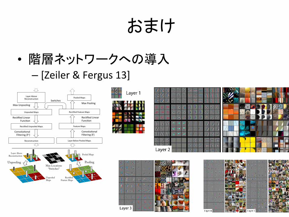
• �3ÙÖØèëɶ³1�(– [Zeiler(&(Fergus(13]�
Visualizing and Understanding Convolutional Networks
invert this, the deconvnet uses transposed versions ofthe same filters, but applied to the rectified maps, notthe output of the layer beneath. In practice this meansflipping each filter vertically and horizontally.
Projecting down from higher layers uses the switchsettings generated by the max pooling in the convneton the way up. As these switch settings are peculiarto a given input image, the reconstruction obtainedfrom a single activation thus resembles a small pieceof the original input image, with structures weightedaccording to their contribution toward to the featureactivation. Since the model is trained discriminatively,they implicitly show which parts of the input imageare discriminative. Note that these projections are notsamples from the model, since there is no generativeprocess involved.
Layer Below Pooled Maps
Feature Maps
Rectified Feature Maps
Convolu'onal)Filtering){F})
Rec'fied)Linear)Func'on)
Pooled Maps
Max)Pooling)
Reconstruction
Rectified Unpooled Maps
Unpooled Maps
Convolu'onal)Filtering){FT})
Rec'fied)Linear)Func'on)
Layer Above Reconstruction
Max)Unpooling)
Switches)
Unpooling Max Locations
“Switches”
Pooling
Pooled Maps
Feature Map
Layer Above Reconstruction
Unpooled Maps
Rectified Feature Maps
Figure 1. Top: A deconvnet layer (left) attached to a con-vnet layer (right). The deconvnet will reconstruct an ap-proximate version of the convnet features from the layerbeneath. Bottom: An illustration of the unpooling oper-ation in the deconvnet, using switches which record thelocation of the local max in each pooling region (coloredzones) during pooling in the convnet.
3. Training Details
We now describe the large convnet model that will bevisualized in Section 4. The architecture, shown inFig. 3, is similar to that used by (Krizhevsky et al.,2012) for ImageNet classification. One di↵erence isthat the sparse connections used in Krizhevsky’s lay-ers 3,4,5 (due to the model being split across 2 GPUs)are replaced with dense connections in our model.
Other important di↵erences relating to layers 1 and2 were made following inspection of the visualizationsin Fig. 6, as described in Section 4.1.
The model was trained on the ImageNet 2012 train-ing set (1.3 million images, spread over 1000 di↵erentclasses). Each RGB image was preprocessed by resiz-ing the smallest dimension to 256, cropping the center256x256 region, subtracting the per-pixel mean (acrossall images) and then using 10 di↵erent sub-crops of size224x224 (corners + center with(out) horizontal flips).Stochastic gradient descent with a mini-batch size of128 was used to update the parameters, starting with alearning rate of 10�2, in conjunction with a momentumterm of 0.9. We anneal the learning rate throughouttraining manually when the validation error plateaus.Dropout (Hinton et al., 2012) is used in the fully con-nected layers (6 and 7) with a rate of 0.5. All weightsare initialized to 10�2 and biases are set to 0.
Visualization of the first layer filters during trainingreveals that a few of them dominate, as shown inFig. 6(a). To combat this, we renormalize each filterin the convolutional layers whose RMS value exceedsa fixed radius of 10�1 to this fixed radius. This is cru-cial, especially in the first layer of the model, where theinput images are roughly in the [-128,128] range. As in(Krizhevsky et al., 2012), we produce multiple di↵er-ent crops and flips of each training example to boosttraining set size. We stopped training after 70 epochs,which took around 12 days on a single GTX580 GPU,using an implementation based on (Krizhevsky et al.,2012).
4. Convnet Visualization
Using the model described in Section 3, we now usethe deconvnet to visualize the feature activations onthe ImageNet validation set.
Feature Visualization: Fig. 2 shows feature visu-alizations from our model once training is complete.However, instead of showing the single strongest ac-tivation for a given feature map, we show the top 9activations. Projecting each separately down to pixelspace reveals the di↵erent structures that excite agiven feature map, hence showing its invariance to in-put deformations. Alongside these visualizations weshow the corresponding image patches. These havegreater variation than visualizations as the latter solelyfocus on the discriminant structure within each patch.For example, in layer 5, row 1, col 2, the patches ap-pear to have little in common, but the visualizationsreveal that this particular feature map focuses on thegrass in the background, not the foreground objects.