EKT3142010‐2011Lab

2013 EKT 314 Electronic Instrumentation

Laboratory Exercise Instructions

Stage I

Prepared By:

Muhamad Asmi bin Romli

asmi@unimap.edu.my

December 2010

EKT3142010‐2011Lab

Content: Lesson Ex.# Content 1: Setting Up Your Hardware 1-1 Concept: MAX

1-2 Concept: GPIB Configuration with MAX 2: Navigating LabVIEW 2-1 Concept: Exploring a VI

2-2 Concept: Navigating Palettes 2-3 Concept: Selecting a Tool 2-4 Concept: Dataflow 2-5 Simple AAP VI

3: Troubleshooting and Debugging VIs 3-1 Concept: Using Help 3-2 Concept: Debugging

4: Implementing a VI 4-1 Determine Warnings VI 4-2 Auto Match VI 4-3 Concept: While Loops versus For Loops 4-4 Average Temperature VI 4-5 Temperature Multiplot VI 4-6 Determine Warnings VI 4-7 Self Study: Square Rect VI 4-8 Self Study: Determine Warnings VI

(Challenge) 4-9 Self Study: Determine More Warnings VI

5: Relating Data 5-1 Concept: Manipulating Arrays 5-2 Concept: Clusters 5-3 Concept: Type Definition

6: Managing Resources 6-1 Spreadsheet Example VI 6-2 Temperature Log VI 6-3 Using DAQmx 6-4 Concept: NI Devsim VI

7: Developing Modular Applications 7-1 Determine Warnings VI 8: Common Design Techniques and Patterns

8-1 State Machine VI

9: Using Variables 9-1 Local Variable VI 9-2 Global Data Project 9-3 Concept: Bank VI

Appendix A A-1 Concept: Analysis Types Appendix B B-1 Concept: Measurement Fundamentals Appendix C C-1 Concept: CAN Device Setup

C-2 Channel Configuration C-3 Read and Write CAN Channels C-4 Synchronize CAN & DAQ

EKT3142010‐2011Lab

EKT314 Electronic Instrumentation Course Mark Exam Work (70%) Final Exam : 50% Test 1: Chapter 1 & 2 (24-30/01/2011) : 10% Test 2: Chapter 3 & 4 (21-27/03/2011) : 10% Course Work (30%)

Log Book (Exercises & Project) : 10% Lab Test (21-27/03/2011) : 10% Lab Project & Viva (28/03 – 17/04/2011) : 10%

EKT3142010‐2011Lab

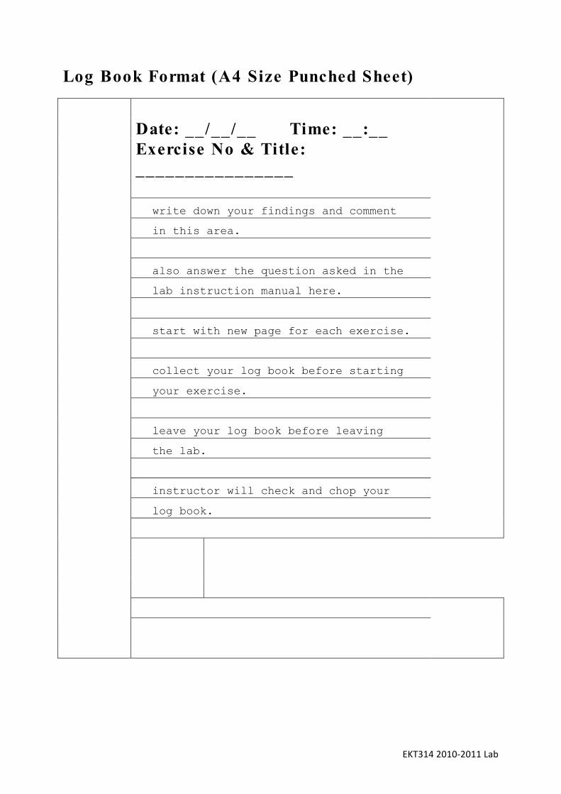
Log Book Format (A4 Size Punched Sheet)

Date: __/__/__ Time: __:__ Exercise No & Title: ________________ D write down your findings and comment D in this area. D D also answer the question asked in the D lab instruction manual here. D start with new page for each exercise. D D collect your log book before starting D your exercise. D leave your log book before leaving D the lab. D instructor will check and chop your D log book.

EKT3142010‐2011Lab

EKT 314 20112-2013 Sem 2 Teaching Plan

Week Date Start Note Laboratory

5 21/03/13 Lesson 2 and lesson 3

6 28/03/13 Lesson 4

7 4/04/13 Lesson 5

11/04/13 mid semester break Lesson 6 and lesson 1

8 18/04/13

9 25/04/13 Lesson 7

10 2/05/13 Lesson 8 & 9

11 9/05/13 Project Wk 1

12 16/05/13 Project Wk 2

13 23/05/13 Viva Project

14 30/05/13

EKT3142010‐2011Lab

General Instruction

1. Refer to Exercises Reference folder before doing each exercise in this exercise instruction. Each chapter got its own presentation slides. Do the exercises when you reach to the related stage.

2. Follow the exercise steps line by line. Don’t skip. Otherwise you’ll lost.

3. Do the exercise on your own pace. No need to hurry. Finish early not meaning you achieve the objective early.

4. Don’t worry when you do mistakes. Mistakes will teach you more.

5. Raise your hand and ask your instructor whenever you have problem.

EKT3142010‐2011Lab

Lesson 1 Setting Up Your Hardware

Instruction: Just Read Through This Part. Our Hardware is Different. Exercise 1-1 Concept: MAX Goal Use MAX to examine, configure, and test a device. Description Complete the following steps to examine the configuration for the DAQ device in the computer using MAX. Use the test routines in MAX to confirm operation of the device. If you do not have a DAQ device, you can simulate a device using the instructions in the Creating a Simulated Device section. Note Portions of this exercise can only be completed with the use of a real device and a DAQ

signal accessory. Some of these steps have alternative instructions for simulated devices.

1. Launch MAX by selecting Start»Programs»National Instruments»Measurement & Automation or by double-clicking the MAX icon on your desktop. MAX searches the computer for installed National Instruments hardware and displays the information. Creating a Simulated Device 2. Create an NI-DAQmx simulated device to allow you to complete the exercises without hardware. Note If you have a DAQ device installed, you can skip this step and go to the Examining the

DAQ Device Settings section.

• Expand Devices and Interfaces . • Right-click NI-DAQmx Devices and select Create New NI-DAQmx

Device»NI-DAQmx Simulated Device . • In the Choose Device dialog box, select M Series DAQ»NI PCI 6225 . • Click the OK button.

EKT3142010‐2011Lab

Examining the DAQ Device Settings l. Expand the Devices and Interfaces section. 2. Expand the NI-DAQmx Devices section to view the installed National Instruments devices that use the NI-DAQmx driver. 3. Select the device listed in the NI-DAQmx Devices section that is connected to your machine. Figure 1-1 shows the NI PCI-6225 and NI USB-6009 devices. Note You might have a different device installed, and some of the options shown might be

different. Click the Show Help/Hide Help button in the top right corner of MAX to hide the online help and show the DAQ device information. However, the Show Help/Hide Help button only appears in certain cases.

Figure 1-1. MAX with Device and Interfaces expanded

MAX displays the National Instruments hardware and software in the computer. The device number appears in quotes following the device name. The Data Acquisition Vls use this device number to determine which device performs DAQ operations. MAX also displays the attributes of the device such as the system resources that the device uses.

EKT3142010‐2011Lab

4. Select the Device Routes tab at the bottom of the dialog to see detailed information about the internal signals that can be routed to other destinations on the device, as shown in Figure 1-2. This is a powerful resource that gives you a visual representation of the signals that are available to provide timing and synchronization with components that are on the device and other external devices.

Figure 1-2 . Device Routes

EKT3142010‐2011Lab

5. Select the Calibration tab, as shown in Figure 1-3, to see information about the last time the device was calibrated both internally and externally.

Figure 1-3 . Calibration

6. Right-click the NI-DAQmx device in the configuration tree and select Self-Calibrate to calibrate the DAQ device using a precision voltage reference source and update the built-in calibration constants. Complete the steps in the dialog that appears. When the device has been calibrated, the Self Calibration information updates in the Calibration tab. Skip this step if you are using a simulated device. Testing the DAQ Device Components l. Click the Self-Test button to test the device. This tests the system resources assigned to the device. The device should pass the test because it is already configured. 2. Click the Test Panels button to test the individual functions of the DAQ device, such as analog input and output. The Test Panels dialog box appears.

• Use the Analog Input tab to test the various analog input channels on the DAQ device. Click the Start button to acquire data from analog input channel 0.

o If you have a DAQ Signal Accessory, channel Dev1/ai0 is connected to the temperature sensor. Place your finger on the sensor to see the voltage rise. You also can move the Noise switch to On on the DAQ Signal Accessory to see the signal change in this tab. When you are finished, click the Stop button.

EKT3142010‐2011Lab

o If you are using a simulated device, a sine wave is shown on all input channels. Experiment with the setting on this tab. When you are finished, click the Stop button.

• Click the Analog Output tab to set up a single voltage or sine wave on one of the DAQ device analog output channels.

• Change the output Mode to Sinewave Generation and click the Start button. MAX generates a continuous sine wave on analog output channel 0. You observe the sine wave in a later step.

• If you have hardware installed, wire Analog Out Ch0 to Analog In Ch1 on the DAQ Signal Accessory.

• If you have hardware installed, click the Analog Input tab and change the channel to Dev1/ai1. Click the Start button to acquire data from analog input channel 1. MAX displays the sine wave from analog output channel 0.

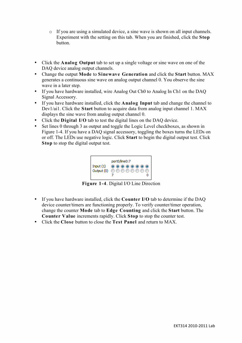
• Click the Digital I/O tab to test the digital lines on the DAQ device. • Set lines 0 through 3 as output and toggle the Logic Level checkboxes, as shown in

Figure 1-4. If you have a DAQ signal accessory, toggling the boxes turns the LEDs on or off. The LEDs use negative logic. Click Start to begin the digital output test. Click Stop to stop the digital output test.

Figure 1-4 . Digital I/O Line Direction

• If you have hardware installed, click the Counter I/O tab to determine if the DAQ device counter/timers are functioning properly. To verify counter/timer operation, change the counter Mode tab to Edge Counting and click the Start button. The Counter Value increments rapidly. Click Stop to stop the counter test.

• Click the Close button to close the Test Panel and return to MAX.

EKT3142010‐2011Lab

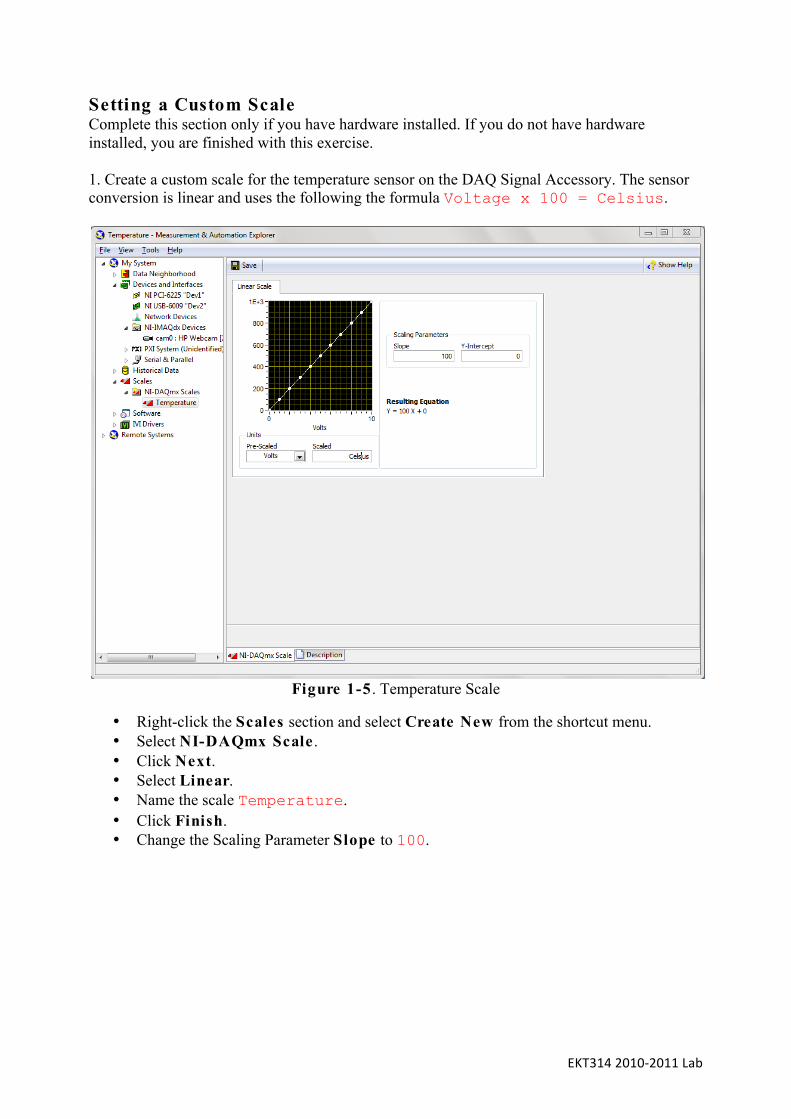
Setting a Custom Scale Complete this section only if you have hardware installed. If you do not have hardware installed, you are finished with this exercise. 1. Create a custom scale for the temperature sensor on the DAQ Signal Accessory. The sensor conversion is linear and uses the following the formula Voltage x 100 = Celsius.

Figure 1-5 . Temperature Scale

• Right-click the Scales section and select Create New from the shortcut menu. • Select NI-DAQmx Scale . • Click Next. • Select Linear. • Name the scale Temperature. • Click Finish. • Change the Scaling Parameter Slope to 100.

EKT3142010‐2011Lab

• Enter Celsius as the Scaled Units . • Click the Save button on the toolbar to save the scale. You use this scale in later

exercises.

2. Close MAX by selecting File»Exit. End of Exercise 1-1

EKT3142010‐2011Lab

Exercise 1-2 Concept: GPIB Contiguration with MAX

Instruction: Just Read Through This Part. We do not have GPIB Instrument. Goal Learn to configure the NI Instrument Simulator and use MAX to examine the GPIB interface settings, detect instruments, and communicate with an instrument. Description This lesson uses one of the following NI Instrument Simulators. Follow the instructions for the Instrument Simulator you are using.

Figure 1-6. NI Instrument Simulator A with DIP Switches

Figure 1-7. Nl Instrument Simulator B Front Panel If you are using NI Instrument Simulator A, shown in Figure 1-6, follow the instructions in Part A of this exercise. If you are using NI Instrument Simulator B, shown in Figure l-7, follow the instructions in Part B of this exercise. Part A: NI Instrument Simulator A Description 1. Configure the NI Instrument Simulator.

• Power off the NI Instrument Simulator. • Set the left bank of switches on the side of the box to match Figure 1-8. • Power on the NI Instrument Simulator.

EKT3142010‐2011Lab

• Verify that both the POWER and READY LEDs are lit.

Figure 1-8. GPIB Configuration Settings for the NI Instrument Simulator A 2. Launch MAX by selecting Start»Programs»National Instruments» Measurement & Automation or by double-clicking the MAX icon on your desktop. 3. View the settings for the GPIB interface.

• Expand the Devices and Interfaces section to display the installed interfaces. If a GPIB interface is listed, the NI-488.2 software is correctly loaded on the computer.

• Select the GPIB interface. • Examine but do not change the settings for the GPIB interface.

4. Communicate with the GPIB instrument.

• Make sure the GPIB interface is still selected in the Devices and Interfaces section. • Click the Scan for Instruments button on the toolbar. • Expand the GPIB interface that is selected in the Devices and Interfaces section.

One instrument named Instrument 0 appears. • Click Instrument 0 to display information about it in the right pane of MAX. Notice

that the NI Instrument Simulator has a GPIB primary address (PAD) of 2. • Click the Communicate with Instrument button on the toolbar. An interactive

window appears. You can use it to query, write to, and read from that instrument.

EKT3142010‐2011Lab

• Enter *IDN? in Send String and click the Query button. The instrument returns its make and model number in String Received as shown in Figure 1-9. You can use this window to debug instrument problems or to verify that specific commands work as described in the instrument documentation.

Figure 1-9. Communication with the GPIB instrument

• Enter MEAS:DC? in Send String and click the Query button. The NI Instrument Simulator returns a simulated voltage measurement.

• Click the Query button again to return a different value. • Click the Exit button when done.

5. Set a VISA alias of devsim for the NI Instrument Simulator so you can use the alias instead of having to remember the primary address.

• While Instrument 0 is selected in MAX, select the VISA Properties tab. • Enter devsim in the VISA Alias on My System field. You will use this alias in

Exercise 6-4. 6. Select File»Exit to exit MAX. 7. Click Yes when prompted to save the instrument.

EKT3142010‐2011Lab

Part B: NI Instrument Simulator B Description 1. Configure the NI Instrument Simulator.

• Power off the NI Instrument Simulator. • Set the configuration switch on the rear panel to CFG. as shown in Figure 1-10.

Figure 1-10. NI Instrument Simulator B

• Power on the NI Instrument Simulator using the power switch on the front of the unit. • Verify that the PWR LED is lit and the RDY LED is flashing. • Launch the NI Instrument Simulator Wizard from Start»Programs»National

Instruments»Instrument Simulator. • Click Next. • Click Next. • Select GPIB Interface and click Next. • Select Change GPIB Settings and click Next. • Select Single Instrument Mode and click Next. • Set GPIB Primary Address to 1. • Set GPIB Secondary Address to 0 (disabled). • Click Next. • Click Update . • Click Back to return and configure the Serial settings. • Select Change Serial Settings and click Next.

EKT3142010‐2011Lab

• Match the serials settings to the settings shown in Figure 1-11.

Figure 1-11. Nl Instrument Simulator Wizard Settings

• Click Next. • Click Update . • Click OK. • Power off the NI Instrument Simulator using the power switch on the front of the unit. • Set the configuration switch on the rear panel to NORM. • Power on the NI Instrument Simulator using the power switch on the front of the unit. • Verify that both the PWR and RDY LEDs are lit.

2. Launch MAX by either double-clicking the icon on the desktop or by selecting Tools»Measurement & Automation Explorer in LabVIEW.

EKT3142010‐2011Lab

3. View the settings for the GPIB interface. • Expand the Devices and Interfaces section to display the installed interfaces. If a

GPIB interface is listed, the NI-488.2 software is correctly loaded on the computer. • Select the GPIB interface. • Examine but do not change the settings for the GPIB interface.

4. Communicate with the GPIB instrument.

• Make sure the GPIB interface is still selected in the Devices and Interfaces section. • Click the Scan for Instruments button on the toolbar. • Expand the GPIB interface that is selected in the Devices and Interfaces section.

One instrument named Instrument 0 appears. • Click Instrument 0 to display information about it in the right pane of MAX. Notice

the NI Instrument Simulator has a GPIB primary address (PAD). • Click the Communicate with Instrument button on the toolbar. An interactive

window appears. You can use it to query, write to, and read from that instrument. • Enter *IDN? in Send String and click the Query button. The instrument returns its

make and model number in String Received as shown in Figure 1-12. You can use this window to debug instrument problems or to verify that specific commands work as described in the instrument documentation.

Figure 1-12. Communication with the GPIB instrument

EKT3142010‐2011Lab

• Enter MEASURE:VOLTAGE:DC? in Send String and click the Query button. The NI Instrument Simulator returns a simulated voltage measurement.

• Click the Query button again to return a different value. • Click the Exit button when done.

5. Set a VISA alias of devsim for the NI Instrument Simulator so you can use the alias instead of having to remember the primary address.

• While Instrument 0 is selected in MAX, select the VISA Properties tab. • Enter devsim in the VISA Alias on My System field. You will use this alias

throughout this lesson. 6. Select File»Exit to exit MAX. 7. Click Yes when prompted to save the instrument. End of Exercise 1-2

EKT3142010‐2011Lab

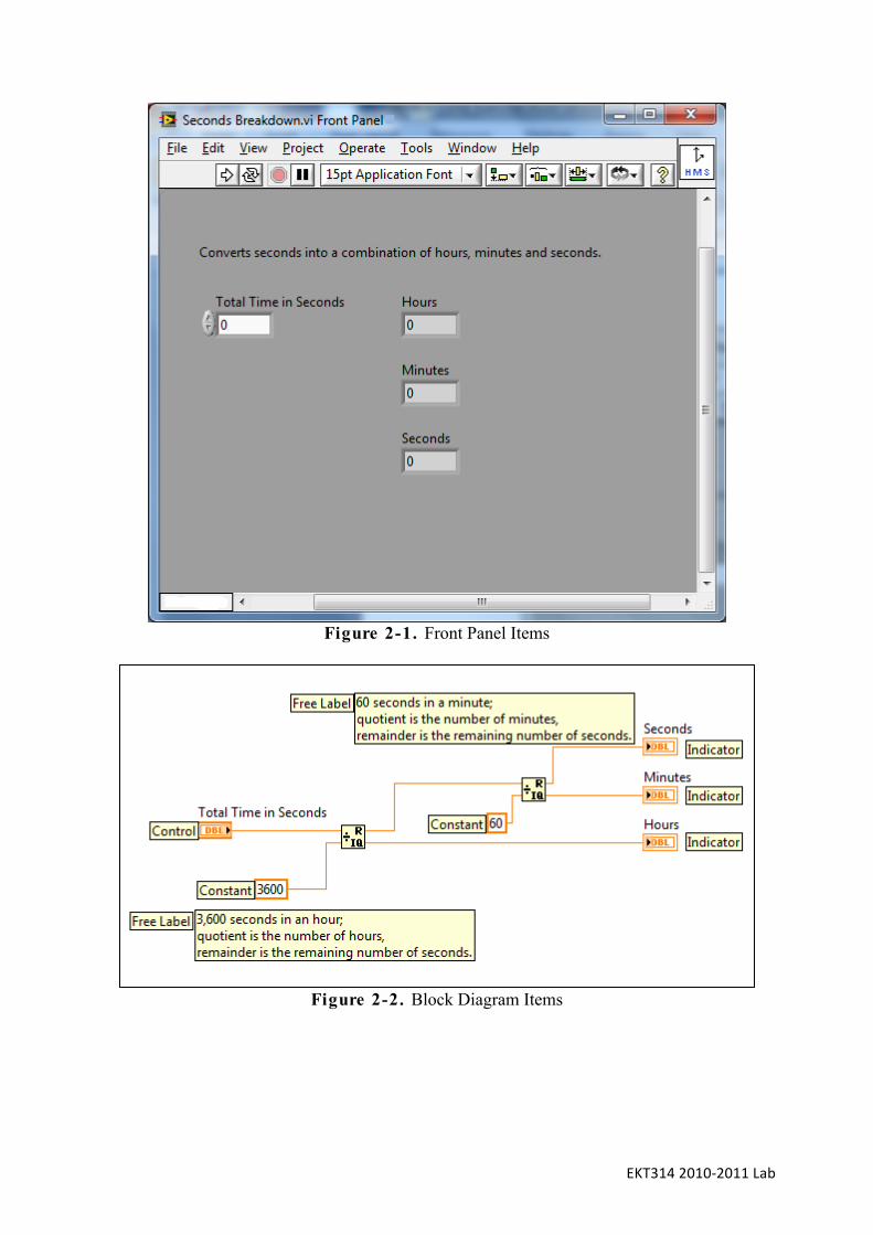
Lesson 2 Navigating LabVIEW Exercise 2-1 Concept: Exploring a VI Goal Identify the parts of an existing VI. Description You received a VI from an employee that takes the seconds until a plane arrives at an airport and converts the time into a combination of hours/minutes/seconds. You must evaluate this VI to see if it works as expected and can display the remaining time until the plane arrives. 1. Open Seconds Breakdown.vi in the <Your_Drive>\Exercises\Exploring A VI directory. 2. On the front panel, identify the following items:

• Control • Indicator • Run button • Icon

3. To view the front panel and block diagram at the same time, select Window»Tile Up and Down. 4. On the block diagram, identify the following items:

• Control • Indicator • Constant • Free Label

To verify that you identified all items correctly, see Figures 2-1 and 2-2.

EKT3142010‐2011Lab

Figure 2-1. Front Panel Items

Figure 2-2. Block Diagram Items

EKT3142010‐2011Lab

5. Test the VI using the values given in Table 2-1. • Enter the input value in the Total Time in Seconds control. • Click the Run button. • For each input, compare the given outputs to the outputs listed in Table 2-1. If the VI

works correctly, they should match.

Table 2-1. Testing Values for Seconds Breakdown.vi Input Output 0 seconds 0 hours, 0 minutes, 0 seconds 60 seconds 0 hours, l minute, 0 seconds 3600 seconds l hour, 0 minutes, 0 seconds 3665 seconds l hour, l minute, 5 seconds End of Exercise 2-1

EKT3142010‐2011Lab

Exercise 2-2 Concept: Navigating Palettes Goal Learn to find controls and functions. Description 1. Open a blank VI and select View»Controls Palette on the front panel window. 2. Explore the Controls palette.

• Click the Search button. • Type string control. • Click a search result and drag it to the front panel window to place the object.

3. Open the block diagram and select View»Functions Palette . 4. Explore the Functions palette.

• Place the DAQ Assistant VI in the Favorites Category. o Locate the DAQ Assistant VI. o On the Measurement I/O subpalette, right-click on the DAQ Assistant VI and

select Add Item to Favorites from the shortcut menu. o Notice that the Favorites category on the Functions palette now contains the

DAQ Assistant VI. 5. Practice accessing similar functions.

• Place an Add function on the block diagram. • Right-click the Add function and notice that a Numeric palette is available. • Practice placing functions from the Numeric palette on the block diagram.

End of Exercise 2-2

EKT3142010‐2011Lab

Exercise 2-3 Concept: Selecting a Tool Goal Become familiar with automatic tool selection in LabVIEW. Description During this exercise, you complete tasks in a partially built tront panel and block diagram. These tasks give you experience using the automatic tool selection. 1. Open Using Temperature.vi.

• Open LabVIEW. • Select File»Open. • Navigate to the <Your_Drive>\Exercises\Using Temperature directory. • Select Using Temperature.vi and click OK.

Figure 2-3 shows an example of the front panel as it appears after your modifications. You increase the size of the waveform graph, rename the numeric control, change the value of the numeric control, and move the pointer on the horizontal pointer slide.

Figure 2-3. Using Temperature VI Front Panel

EKT3142010‐2011Lab

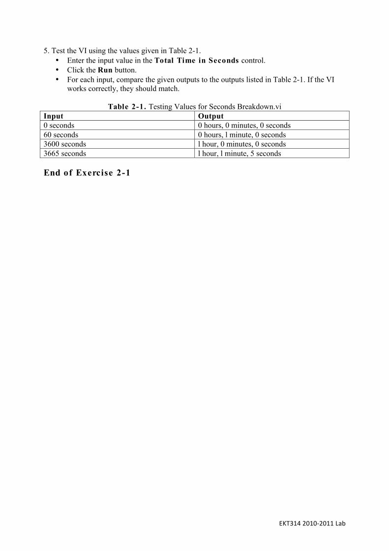
2. Expand the waveform graph horizontally using the Positioning tool. • Move the cursor to the left edge of the Waveform Graph. • Move the cursor to the middle left resizing node until the cursor changes to a double

arrow, shown in Figure 2-4.

Figure 2-4. Resize Waveform Graph

• Drag the repositioning point until the Waveform Graph is the size you want.

3. Rename the numeric control to Number of Measurements using the Labeling Tool.

• Move the cursor to the text Numeric. • Double click the word Numeric. • Enter the text Number of Measurements. • Complete the entry by clicking the Enter Text button on the toolbar, or clicking

outside the control. 4. Change the value of the Number of Measurements control to 20 using the Labeling tool.

• Move the cursor to the interior of the numeric control. • When the cursor changes to the Labeling tool icon, as shown at left, click the mouse

button. • Enter the text 20. • Complete the entry by pressing the <Enter> key on the numeric keypad, clicking the

Enter Text button on the toolbar, or clicking outside the control.

EKT3142010‐2011Lab

5. Change the value of the pointer on the horizontal pointer slide using the Operating tool. • Move the cursor to the pointer on the slide. • When the cursor changes to the Operating tool icon, as shown at left, press the mouse

button and drag to the value you want. • Set the value to 2.

6. Try changing the value of objects, resizing objects, and renaming objects until you are comfortable with using these tools. Figure 2-5 shows an example of the block diagram as it appears after your modifications. You move the Number of Measurements terminal and wire the terminal to the count terminal of the For Loop.

Figure 2-5. Using Temperature VI Block Diagram

7. Open the block diagram. 8. Move the Number of Measurements terminal using the Positioning tool.

• Move the cursor to the Number of Measurements terminal. • Move the cursor in the terminal until the cursor changes to an arrow, shown at left. • Click and drag the terminal to the new location as shown in Figure 2-5.

EKT3142010‐2011Lab

9. Wire the Number of Measurements terminal to the count terminal of the For Loop using the Wiring tool.

• Move the cursor to the Number of Measurements terminal. • Move the cursor to the right of the terminal, stopping when the cursor changes to a

wiring spool, as shown at left. • Click to start the wire. • Move the cursor to the count (N) terminal of the For Loop. • Click the count terminal to end the wire.

10. Click the Run button to run the VI. The time required to execute this VI is equivalent to Number of Measurements times Delay (Sec) . Once the VI is finished executing, the data is displayed on the Temperature Graph. 11. Try moving other objects, deleting wires and rewiring them, and wiring objects and wires together until you are comfortable with using these tools. 12. Select File»Close to close the VI and click the Don’t save - All button. You do not need to save the VI. End of Exercise 2-3

EKT3142010‐2011Lab

Exercise 2-4 Concept: Dataflow Goal Understand how dataflow determines the execution order in a VI. Description 1. Open the Dataflow.exe simulation from the <Your_Drive>\Exercises\Dataflow directory. 2. Follow the instructions given. This simulation demonstrates dataflow. End of Exercise 2-4

EKT3142010‐2011Lab

Exercise 2-5 Simple AAP VI Goal Create a simple VI that acquires, analyzes, and presents data. Scenario You need to acquire a sine wave for 0.1 seconds, determine and display the average value, log the data, and display the sine wave on a graph. Design The input for this problem is an analog channel of sine wave data. The outputs include a graph of the sine data and a tile that logs the data. Flowchart

Figure 2-6. Simple AAP VI Flowchart.

EKT3142010‐2011Lab

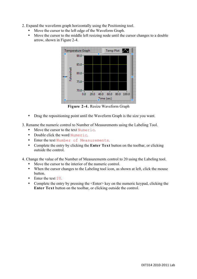
Program Architecture Quiz 1. Acquire: Circle the Express VI that is best suited to acquiring a sine wave from a data acquisition device.

DAQ Assistant

The DAQ Assistant acquires data through a data acquisition device.

Instrument I/O Assistant

The Instrument I/O Assistant acquires instrument control data, usually from a GPIB or serial interface.

Simulate Signal

The Simulate Signal Express VI generates simulated data, such as a sine wave.

2. Analyze: Circle the Express VI that is best suited to determining the average value of the acquired data.

Tone Measurements

The Tone Measurements Express VI finds the frequency and amplitude of a single tone.

Statistics

The Statistics Express VI calculates statistical data from a waveform.

Amplitude and Level Measurements

The Amplitude and Level Measurements Express VI performs voltage measurements on a signal.

Filter

The Filter Express VI processes a signal through filters and windows.

EKT3142010‐2011Lab

3. Present: Circle the Express VIs and/or indicators that are best suited to displaying the data on a graph and logging the data to file.

DAQ Assistant

The DAQ Assistant acquires data through a data acquisition device.

Write to Measurement File

The Write to Measurement File Express VI writes a file in LVM or TDM file format.

Build Text

The Build Text Express VI creates text, usually for displaying on the front panel window or exporting to a file or instrument.

Waveform Graph The waveform graph displays one or more plots of evenly sampled measurements.

Refer to the next page for answers to this quiz.

EKT3142010‐2011Lab

Program Architecture - Quiz Answers 1. Acquire: Use the DAQ Assistant to acquire the sine wave from the data acquisition device. 2. Analyze : Use the Statistics Express VI to determine the average value of the sine wave. Because this signal is cyclical, you could also use the Cycle Average option in the Amplitude and Level Measurements Express VI to determine the average value of the sine wave. 3. Present: Use the Write to Measurement File Express VI to log the data and use the Waveform Graph to display the data on the front panel window.

EKT3142010‐2011Lab

Implementation 1. Prepare your hardware to generate a sine wave. If you are not using hardware, skip to step 2.

• Find the DAQ Signal Accessory and visually confirm that it is connected to the DAQ device in your computer.

• Using a wire, connect the Analog In Channel 1 to the Sine Function Generator, as shown in Figure 2-7.

• Set the Frequency Range switch and the Frequency Adjust knob to their lowest levels.

Figure 2-7. Connection for the DAQ Signal Accessory

2. Open LabVIEW. 3. Open a blank VI.

EKT3142010‐2011Lab

4. Save the VI as Simple AAP.vi. • Select File»Save . • Navigate to the <Your_Drive>\Exercises\Simple AAP directory. • Name the VI Simple AAP.vi. • Click OK.

In the following steps, you will build a front panel window similar to the one in Figure 2-8.

Figure 2-8. Acquire, Analyze and Present Front Panel Window

5. Add a waveform graph to the front panel window to display the acquired data.

• If the Controls palette is not already open, select View»Controls Palette from the LabVIEW menu.

• On the Controls palette, select the Express category. • Select the Graph Indicators category from within the Express category. • Select the waveform graph. • Add the graph to the front panel window.

EKT3142010‐2011Lab

6. Add a numeric indicator to the front panel window to display the average value. • Collapse the Graph Indicators category by selecting Express on the Controls

palette. • Select the Numeric Indicators category from within the Express category. • Select the numeric indicator. • Place the indicator on the front panel. • Enter Average Value in the label of the numeric indicator.

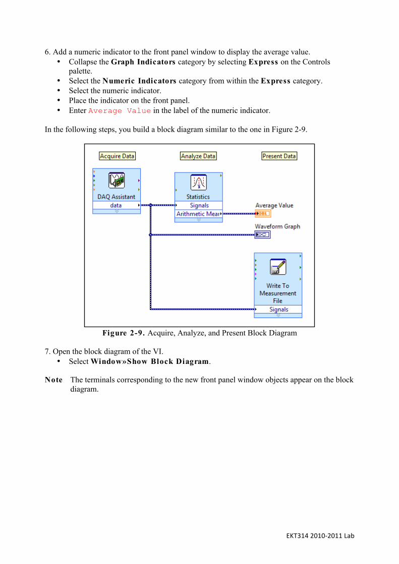
In the following steps, you build a block diagram similar to the one in Figure 2-9.

Figure 2-9. Acquire, Analyze, and Present Block Diagram

7. Open the block diagram of the VI.

• Select Window»Show Block Diagram. Note The terminals corresponding to the new front panel window objects appear on the block

diagram.

EKT3142010‐2011Lab

8. Acquire a sine wave for 0.1 seconds. If you have hardware installed, follow the instructions in the Hardware Installed column to acquire the data using the DAQ Assistant. If you do not have hardware installed, follow the instructions in the No Hardware Installed column to simulate the acquisition using the Simulate Signal Express VI.

Hardware Installed No Hardware Installed 1. On the Functions palette, select the

Express category. 1. On the Functions palette, select the

Express category. 2. Select Input from the Express category. 2. Select Input from the Express category. 3. Select the DAQ Assistant from the

Input category. 3. Select Simulate Signal from the Input

category. 4. Place the DAQ Assistant on the block

diagram. 4. Place the Simulate Signal Express VI on

the block diagram. 5. Wait for the DAQ Assistant dialog box to

open. 5. Wait for the Simulate Signal dialog box to

open. 6. Select Acquire Signals»Analog

Input»Voltage for the measurement type.

6. Select Sine for the signal type.

7. Select ai1 (analog input channel 1) for the physical channel.

7. Set the signal frequency to 100.

8. Click the Finish button. 8. In the Timing section, set the Samples per second (Hz) to 1000.

9. In the Timing Settings section, select N Samples as the Acquisition Mode .

9. In the Timing section, deselect Automatic for the Number of samples.

10. In the Timing Settings section enter 100 in Samples To Read.

10. In the Timing section, set the Number of samples to 100.

11. Enter 1000 in Rate (Hz) . 11. Select the Simulate acquisition timing selection.

12. Click the OK button. 12. Click the OK button. Tip Reading 100 samples at a rate of 1,000 Hz retrieves 0.1 seconds worth of data.

EKT3142010‐2011Lab

9. Determine the average value of the data acquired by using the Statistics Express VI. • Collapse the Input palette by selecting Express on the Functions palette. • Select the Signal Analysis palette. • Select the Statistics Express VI and add the Statistics Express VI to the block diagram

to the right of the DAQ Assistant. • Wait for the Statistics Express VI dialog box to open. • Enable the Arithmetic mean checkbox. • Click the OK button.

10. Log the generated sine data to a LabVIEW Measurement File.

• Select Express on the Functions palette. • Select the Output category. • Select Write to Measurement File . • Add the Write to Measurement File Express VI to the block diagram below the

Statistics Express VI. • Wait for the Write to Measurement File Express VI dialog box to open. • Leave all settings as default. • Click the OK button.

Note Future exercises do not detail the directions for finding specific functions or controls in

the palettes. Use the palette search feature to locate functions and controls. 11. Wire the data from the DAQ Assistant (or Simulate Signal Express VI) to the Statistics Express VI.

• Place the mouse cursor over the data output of the DAQ Assistant (or the Sine output of the Simulate Signal Express VI) at the location where the cursor changes to the Wiring tool.

EKT3142010‐2011Lab

• Click the mouse button to start the wire. • Place the mouse cursor over the Signals input of the Statistics Express VI and click the

mouse button to end the wire. 12. Wire the data to the graph indicator.

• Place the mouse cursor over the data output wire of the DAQ Assistant (or the Sine output of the Simulate Signal Express VI) at the location where the cursor changes to the Wiring tool.

• Click the mouse button to start the wire. • Place the mouse cursor over the Waveform Graph indicator and click the mouse button

to end the wire. 13. Wire the Arithmetic Mean output of the Statistics Express VI to the Average Value numeric indicator.

• Place the mouse cursor over the Arithmetic Mean output of the Statistics Express VI at the location where the cursor changes to the Wiring tool.

• Click the mouse button to start the wire. • Place the mouse cursor over the Average Value numeric indicator and click the

mouse button to end the wire. 14. Wire the data output to the Signals input of the Write Measurement File Express VI.

• Place the mouse cursor over the data output wire of the DAQ Assistant (or the Sine output of the Simulate Signal Express VI) at the location where the cursor changes to the Wiring tool.

• Click the mouse button to start the wire. • Place the mouse cursor over the Signals input of the Write Measurement File Express

VI and click the mouse button to end the wire. Note Future exercises do not detail the directions for wiring between objects. 15. Save the VI.

EKT3142010‐2011Lab

Test 1. Switch to the front panel window of the VI. 2. Set the graph properties to be able to view the sine wave.

• Right-click the waveform graph and select X Scale»Autoscale X to disable autoscaling.

• Right-click the waveform graph and select Visible Items»X Scrollbar to enable the X scale.

• Use the labeling tool to change the last number on the X Scale of the waveform graph to .1.

3. Save the VI. 4. Run the VI.

• Click the Run button on the front panel toolbar. The graph indicator should display a sine wave and the Average Value indicator should display a number around zero. If the VI does not run as expected, review the implementation steps.

5. Close the VI. End of Exercise 2-5

EKT3142010‐2011Lab

Lesson 3: Troubleshooting and Debugging VIs Exercise 3-1 Concept: Using Help Goal Become familiar with using the Context Help window, the LabVIEW Help, and the NI Example Finder. Description This exercise consists of a series of tasks designed to help you become familiar with the LabVIEW Help tools. NI Example Finder 1. You have a DAQ device in your computer, and you want to learn how to communicate with it using LabVIEW. Use the NI Example Finder to find a VI that communicates with a DAQ device.

• Open LabVIEW. • Select Help»Find Examples to open the NI Example Finder. • Confirm that the Task option is selected on the Browse tab. • Double-click the Hardware Input and Output folder. • Select DAQmx»Analog Measurements»Voltage . • Select Acq&Graph Voltage-Int Clk.vi . Notice that a description of the VI is

provided in the Information text box so that you can verify that this VI meets your needs.

• Double-click Acq&Graph Voltage-Int Clk.vi to open the VI. • Close the VI after you finish exploring it.

2. You want to learn more about using Express Vls to filter signals. Use the NI Example Finder to find an appropriate VI.

• The NI Example Finder should still be open from the previous step. If not, open the NI Example Finder.

• Click the Search tab in the NI Example Finder.

EKT3142010‐2011Lab

• Enter express in the Enter keyword(s) field to find Vls that contain Express Vls. • Double-click the Express result that appears in the Double-click keyword(s)

field. • This keyword is associated with many example Vls. as demonstrated by the number of

Vls returned. You can select any one of these Vls and read the description in the Information text box.

• Double-click Express Filter.vi to open it. Context Help Window 3. Use the Context Help window to learn about the Express Vls used in the Express Filter VI.

• Open the block diagram by selecting Window»Show Block Diagram. • Open the Context Help window by selecting Help»Show Context Help. • Move the Context Help window to a convenient area where the window does not hide

part of the block diagram. • Place your mouse cursor over the Simulate Signal Express Vl. The Context Help

window content changes to show information about the object that your mouse is over. • Move your mouse over another Express VI. Notice the Context Help window content

changes corresponding to the location of the mouse cursor. • Move your mouse over one of the Tone Measurements Express Vls. • Examine the configuration details in the Context Help window. This gives you the

information about how the Express VI is configured. • Double-click the Tone Measurements Express VI to open the configuration dialog box.

Notice that the selections in the configuration dialog box match the information in the Context Help window.

• Click the OK button to close the configuration dialog box.

EKT3142010‐2011Lab

4. Anchor the Context Help window so that you can move your mouse without the contents of the window changing. The Context Help window should show information about the Simulate Signal Express VI.

• Move your mouse over the Simulate Signal Express VI. • To anchor the context help window, select the Lock button in the lower left corner of

the window. Tip If the contents of the window change before you lock the window, avoid passing your

mouse over other objects on the way to the Context Help window. Move the window closer to the object of interest to view Context Help for that item.

• Move your mouse over another object. Notice the contents of the window do not change

while the Lock button is selected. • Deselect the Lock button to resume normal operation of the window.

5. Modify the Description and Tip associated with the Simulated frequency control to change the content shown in the Context Help window.

• Select Window»Show Front Panel to open the front panel of the VI. • Move your mouse over the Simulated frequency control. • Read the contents of the Context Help window. • Right-click the Simulated frequency control. • Select Description and Tip from the shortcut menu. • Replace the text in the "Simulated frequency" Description box with the text:

This is the description of the control. • Replace the text in the "Simulated frequency" Tip box with the text: This is

the tip for the control. • Click the OK button. • Move your mouse over the Simulated frequency control. • Notice that the contents of the Context Help window changed to match the text you

typed in the Description field of the Description and Tip dialog box. • Run the VI.

EKT3142010‐2011Lab

• Place your mouse cursor over the Simulated frequency control. • Notice that the tool tip that appears matches the text you typed in the Tip field of the

Description and Tip dialog box. • Click the Stop button.

LabVIEW Help 6. Use the LabVIEW Help to learn more information about the Filter Express VI.

• Select Window»Show Block Diagram to open the block diagram of the Express Filter VI.

• Right-click the Filter Express VI and select Help from the shortcut menu. This opens the LabVIEW Help topic for the Filter Express VI.

Note To access the LabVIEW Help for this topic, you can also select the Detailed Help link

in the Context Help window while the Filter Express VI is selected, or click the question mark in the Context Help window.

• Explore the topic. For example, what is the purpose of the Cutoff Frequency (Hz)

dialog box option? • Close the LabVIEW Help window.

7. Close the Express Filter VI when you finish. Do not save changes. End of Exercise 3-1

EKT3142010‐2011Lab

Exercise 3-2 Concept: Debugging Goal Use the debugging tools built into LabVIEW. Description Complete the following steps to load a broken VI and correct the errors. Use single-stepping and execution highlighting to step through the VI. 1. Open and examine the Debug Exercise (Main) VI.

• Select File»Open. • Open Debug Exercise (Main).vi in the

<Your_Drive>\Exercises\Debugging directory. The following front panel appears.

Figure 3-1. Debug Exercise (Main).vi Front Panel

• Notice the Run button on the toolbar appears broken, indicating that the VI is broken

and cannot run.

EKT3142010‐2011Lab

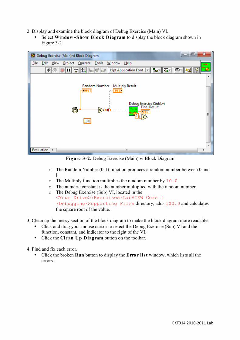
2. Display and examine the block diagram of Debug Exercise (Main) VI. • Select Window»Show Block Diagram to display the block diagram shown in

Figure 3-2.

Figure 3-2. Debug Exercise (Main).vi Block Diagram

o The Random Number (0-1) function produces a random number between 0 and

l. o The Multiply function multiplies the random number by 10.0. o The numeric constant is the number multiplied with the random number. o The Debug Exercise (Sub) VI, located in the

<Your_Drive>\Exercises\LabVIEW Core 1 \Debugging\Supporting Files directory, adds 100.0 and calculates the square root of the value.

3. Clean up the messy section of the block diagram to make the block diagram more readable.

• Click and drag your mouse cursor to select the Debug Exercise (Sub) VI and the function, constant, and indicator to the right of the VI.

• Click the Clean Up Diagram button on the toolbar. 4. Find and fix each error.

• Click the broken Run button to display the Error list window, which lists all the errors.

EKT3142010‐2011Lab

• Select an error description in the Error list window. The Details section describes the error and in some cases recommends how to correct the error.

• Click the Help button to display a topic in the LabVIEW Help that describes the error in detail and includes step-by-step instructions for correcting the error.

• Click the Show Error button or double-click the error description to highlight the area on the block diagram that contains the error.

• Use the Error list window to fix each error. 5. Select File»Save to save the VI. 6. Display the front panel by clicking it or by selecting Window»Show Front Panel . 7. Click the Run button. 8. Select Window»Show Block Diagram to display the block diagram. 9. Animate the flow of data through the block diagram.

• Click the Highlight Execution button on the toolbar to enable execution highlighting.

• Click the Step Into button to start single-stepping. Execution highlighting shows the flow of data on the block diagram from one node to another using bubbles that move along the wires. Nodes blink to indicate they are ready to execute.

• Click the Step Over button after each node to step through the entire block diagram. Each time you click the Step Over button, the current node executes and pauses at the next node.

• Data appear on the front panel as you step through the VI. The VI generates a random number and multiplies it by 10.0. The subVI adds 100.0 and calculates the square root of the result.

• When a blinking border surrounds the entire block diagram, click the Step Out button to stop single-stepping through the Debug Exercise (Main) VI.

EKT3142010‐2011Lab

10. Single-step through the VI and its subVI. • Click the Step Into button to start single-stepping. • When the Debug Exercise (Sub) VI blinks, click the Step Into button. Notice the Run

button on the subVI. • Display the Debug Exercise (Main) VI block diagram by clicking it. A green glyph

appears on the subVI icon on the Debug Exercise (Main) VI block diagram, indicating that the subVI is running.

• Display the Debug Exercise (Sub) VI block diagram by clicking it. • Click the Step Out button twice to finish single-stepping through the subVI block

diagram. The Debug Exercise (Main) VI block diagram is active. • Click the Step Out button to stop single-stepping.

11. Use a probe to check intermediate values on a wire as a VI runs.

• From the Tools palette, select the Probe tool. • Use the Probe tool to click any wire. The Probe Watch Window appears.

The Probe Watch Window displays all probes in all VIs currently in memory. This window sorts the probes in the order you create them and lists the probes under the VI they belong to.

• Single-step through the VI again. The Probe Watch Window displays data passed along the wire.

12. Place breakpoints on the block diagram to pause execution at that location.

• Use the Breakpoint tool to click nodes or wires. Place a breakpoint on the block diagram to pause execution after all nodes on the block diagram execute.

• Click the Run button to run the VI. When you reach a breakpoint during execution, the VI pauses and the Pause button on the toolbar appears red.

EKT3142010‐2011Lab

• Click the Continue button to continue running to the next breakpoint or until the VI finishes running.

• Use the Breakpoint tool to click the breakpoints you set and remove them. 13. Click the Highlight Execution button to disable execution highlighting. 14. Select File»Close to close the Vl and all open windows. End of Exercise 3-2

EKT3142010‐2011Lab

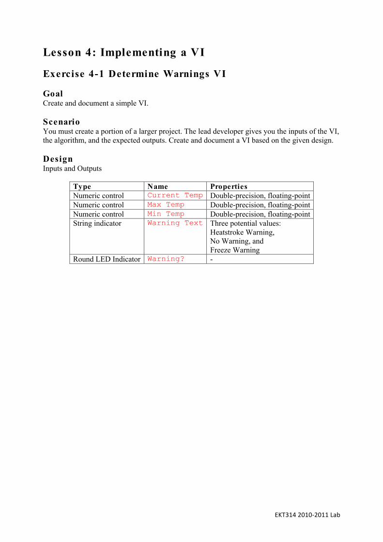
Lesson 4: Implementing a VI Exercise 4-1 Determine Warnings VI Goal Create and document a simple VI. Scenario You must create a portion of a larger project. The lead developer gives you the inputs of the VI, the algorithm, and the expected outputs. Create and document a VI based on the given design. Design Inputs and Outputs

Type Name Properties Numeric control Current Temp Double-precision, floating-point Numeric control Max Temp Double-precision, floating-point Numeric control Min Temp Double-precision, floating-point String indicator Warning Text

Three potential values: Heatstroke Warning, No Warning, and Freeze Warning

Round LED Indicator Warning? -

EKT3142010‐2011Lab

Flowchart

Figure 4-1. Determine Warnings VI Flowchart

EKT3142010‐2011Lab

Implementation Follow the instructions given below to create a front panel similar to Figure 4-2. The user enters the current temperature, maximum temperature, and minimum temperature. Then, the front panel displays the warning string and the warning Boolean LED. This VI is part of the temperature weather station project studied throughout the course. 1. Open a blank VI and create the following front panel.

Figure 4-2. Determine Warnings VI Front Panel

2. Save the new VI.

• Select File»Save . • Save the VI as Determine Warnings.vi in the

<Your_Drive>\Exercises\Determine Warnings directory. 3. Create a numeric control for the current temperature.

• Add a numeric control to the front panel window. • Change the label of the numeric control to Current Temp. • Right-click the control, select Representation, and confirm that the representation

type is set to double precision. Tip This subVI could be used for Fahrenheit, Kelvin, or any other temperature scale, as long

as all inputs use the same scale. Therefore, it is not necessary to add scale units to the labels.

EKT3142010‐2011Lab

4. Create a numeric control for the maximum temperature. • Hold down the <Ctrl> key and click and drag the Current Temp numeric control to

create a copy of the control. • Change the label text of the new numeric control to Max Temp.

5. Create a numeric control for the minimum temperature.

• Hold down the <Ctrl> key and click and drag the Max Temp numeric control to create a copy of the control.

• Change the label text of the new numeric control to Min Temp. 6. Create a string indicator for the warning text.

• Add a string indicator to the front panel window. • Change the label text of the string indicator to Warning Text.

7. Create a Round LED or other Boolean indicator for the warning Boolean.

• Add a Round LED to the front panel window. • Change the label text of the Boolean indicator to Warning?.

8. Switch to the block diagram. Tip If you do not want to view terminals as icons on the block diagram, Select

Tools»Options , then select Block Diagram from the Category list. Remove the checkmark from the Place front panel terminals as icons item.

EKT3142010‐2011Lab

Complete the following instructions to create a block diagram similar to Figure 4-3.

Figure 4-3. Determine Warnings VI Block Diagram

9. Compare Current Temp and Mex Temp.

• Add a Greater Or Equal? function to the block diagram. • Wire the Current Temp control to the x input of the Greater Or Equal? function. • Wire the Max Temp control to the y input of the Greater Or Equal? function.

10. Compare Current Temp and Min Temp.

• Add a Less Or Equal? function to the block diagram. • Wire the Current Temp control to the x input of the Less Or Equal? function. • Wire the Min Temp control to the y input of the Less Or Equal? function.

11. If the Current Temp is equal to or greater than the Max Temp, generate a Heatstroke Warning string, otherwise generate a No Warning String.

• Add the Select function to the block diagram to the right of the Greater Or Equal? function.

• Wire the output of the Greater Or Equal? function to the s input of the Select function.

EKT3142010‐2011Lab

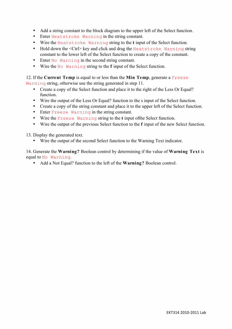
• Add a string constant to the block diagram to the upper left of the Select function. • Enter Heatstroke Warning in the string constant. • Wire the Heatstroke Warning string to the t input of the Select function. • Hold down the <Ctrl> key and click and drag the Heatstroke Warning string

constant to the lower left of the Select function to create a copy of the constant. • Enter No Warning in the second string constant. • Wire the No Warning string to the f input of the Select function.

12. lf the Current Temp is equal to or less than the Min Temp, generate a Freeze Warning string, otherwise use the string generated in step 11.

• Create a copy of the Select function and place it to the right of the Less Or Equal? function.

• Wire the output of the Less Or Equal? function to the s input of the Select function. • Create a copy of the string constant and place it to the upper left of the Select function. • Enter Freeze Warning in the string constant. • Wire the Freeze Warning string to the t input ofthe Select function. • Wire the output of the previous Select function to the f input of the new Select function.

13. Display the generated text.

• Wire the output of the second Select function to the Warning Text indicator. 14. Generate the Warning? Boolean control by determining if the value of Warning Text is equal to No Warning.

• Add a Not Equal? function to the left of the Warning? Boolean control.

EKT3142010‐2011Lab

• Wire the output of the second Select function to the x input of the Not Equal? function. • Wire the No warning string constant to the y input of the Not Equal? function. • Wire the output of the Not Equal? function to the Warning? control.

15. Document the code using the following suggestions on the front panel.

• Create tip strips for each control and indicator stating the purpose and units of the object. To access tip strips, right-click an object, and select Description and Tip.

• Document the VI Properties , giving a general description of the VI, a list of inputs and outputs, your name, and the date the VI was created. To access the VI Properties dialog box, select File»VI Properties .

• Document the block diagram algorithm with a free label. 16. Save the VI. Test 1. Test the VI by entering a value for Current Temp, Max Temp, and Min Temp, and running the VI for each set. Table 4-1 shows the expected Warning Text string and Warning? Boolean value for each set of input values.

Table 4-1. Testing Values for Determine Warnings VI Current Temp Max Temp Min Temp Warning Text Warning? 30 30 10 Heatstroke

Warning True

25 30 10 No Warning False 10 30 10 Freeze Warning True

What happens if you input a Max Temp value that is less than the Min Temp? What would you expect to happen? You learn to handle issues like this one in Exercise 4-6. 2. Save and close the VI. End of Exercise 4-1

EKT3142010‐2011Lab

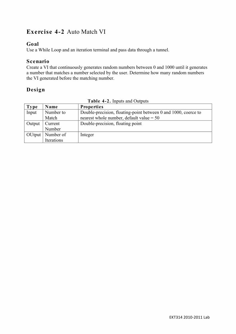
Exercise 4-2 Auto Match VI Goal Use a While Loop and an iteration terminal and pass data through a tunnel. Scenario Create a VI that continuously generates random numbers between 0 and 1000 until it generates a number that matches a number selected by the user. Determine how many random numbers the VI generated before the matching number. Design

Table 4-2. Inputs and Outputs Type Name Properties Input Number to

Match Double-precision, floating-point between 0 and 1000, coerce to nearest whole number, default value = 50

Output Current Number

Double-precision, floating point

OUtput Number of Iterations

Integer

EKT3142010‐2011Lab

Flowchart

Figure 4-4. Auto Match Flowchart

EKT3142010‐2011Lab

Implementation Build the following front panel and modify the controls and indicators as shown on the front panel in Figure 4-5 and described in the following steps.

Figure 4-5. Auto Match VI Front Panel

1. Open a blank VI. 2. Save the Vl as Auto Match.vi in the <Your Drive>\Exercises\Auto Match directory. 3. Create the Number to Match input.

• Add a numeric control to the front panel window. • Label the control Number to Match.

4. Set the default value for the Number to Match control.

• Set the Number to Match control to 50. • Right-click the Number to Match control and select Data Operations»Make

Current Value Default. 5. Set the properties for the Number to Match control so that the data range is from 0 to 1000, the increment value is 1, and the digits of precision is 0.

• Right-click the Number to Match control and select Data Entry from the shortcut menu. The Data Entry page of the Numeric Properties dialog box appears.

• Disable the Use Default Limits checkbox. • Set the Minimum value to 0 and select Coerce from the Response to value

outside limits pull-down menu.

EKT3142010‐2011Lab

• Set the Maximum value to 1000 and select Coerce from the Response to value outside limits pull-down menu.

• Set the Increment value to 1 and select Coerce to Nearest from the Response to value outside limits pull-down menu.

• Select the Display Format tab. • Select Floating Point and change Precision Type from Significant digits to

Digits of precision. • Enter 0 in the Digits text box and click the OK button.

6. Create the Current Number output.

• Add a numeric indicator to the front panel window. • Label the indicator Current Number.

7. Set the digits of precision for the Current Number output to 0.

• Right-click the Current Number indicator and select Display Format from the shortcut menu. The Display Format page of the Numeric Properties dialog box appears.

• Select Floating Point and change Precision Type to Digits of precision. • Enter 0 in the Digits text box and click the OK button.

8. Create the # of iterations output.

• Place a numeric indicator on the front panel. • Label the indicator # of iterations.

9. Set the representation for the # of iterations output to a long integer.

• Right-click the # of iterations indicator. • Select Representation»I32 from the shortcut menu.

EKT3142010‐2011Lab

Create the following block diagram. Refer to the following steps for instructions.

Figure 4-6. Auto Match VI Block Diagram

10. Generate a random number integer between 0 and 1000.

• Add the Random Number (0-1) function to the block diagram. The Random Number (0-1) function generates a random number between 0 and 1.

• Add the Multiply function to the block diagram. The Multiply function multiplies the random number by the y input to produce a random number between 0 and y .

• Wire the output of the Random Number function to the x input of the Multiply function. • Right-click the y input of the Multiply function, select Create»Constant from the

shortcut menu, enter 1000, and press the <Enter> key to create a numeric constant. • Add the Round To Nearest function to the block diagram. This function rounds the

random number to the nearest integer. • Wire the output of the Multiply function to the input of the Round To Nearest function. • Wire the output of the Round To Nearest function to the Current Number indicator.

EKT3142010‐2011Lab

11. Compare the randomly generated number to the value in the Number to Match control. • Add the Not Equal? function to the block diagram. This function compares the random

number with Number to Match and returns True if the numbers are not equal; otherwise, it returns False .

• Wire the output of the Round To Nearest function to the x input of the Not Equal? function.

12. Repeat the algorithm until the Not Equal? function returns True .

• Add a While Loop from the Structures palette to the block diagram. • Right-click the conditional terminal and select Continue if True from the shortcut

menu. • Wire the Number to Match numeric control to the border of the While Loop. An orange

tunnel appears on the While Loop border. • Wire the orange tunnel to the y input of the Not Equal? function. • Wire the output of the Not Equal? function to the conditional terminal.

13. Display the number of random numbers generated to the user by adding one to the iteration terminal value.

• Wire the iteration terminal to the border of the While Loop. A blue tunnel appears on the While Loop border.

Tip Each time the loop executes, the iteration terminal increments by one. you must wire the

iteration value to the Increment function because the iteration count starts at 0.The iteration count passes out of the loop upon completion.

• Add the Increment function to the block diagram. This function adds l to the While

Loop count. • Wire the blue tunnel to the Increment function. • Wire the Increment function to the # of iterations indicator.

l4. Save the VI.

EKT3142010‐2011Lab

Test 1. Display the front panel. 2. Change the number in Number to Match to a number that is in the data range, which is 0 to 1000 with an increment of 1. 3. Right-click the Current Number indicator and select Advanced»Synchronous Display . Note If synchronous display is enabled, then every time the block diagram sends a value to

the Current Number indicator, the block diagram will stop executing until the front panel has updated the value of the indicator. In this exercise, you enable the synchronous display, so you can see the Current Number indicator get updated repeatedly on the front panel. Typically, the synchronous display is disabled to increase execution speed since you usually do not need to see every single updated value of an indicator on the front panel.

4. Run the VI. 5. Change Number to Match and run the VI again. Current Number updates at every iteration of the loop because it is inside the loop. # of iterations updates upon completion because it is outside the loop. 6. To see how the VI updates the indicators, enable execution highlighting.

• On the block diagram toolbar, click the Highlight Execution button to enable execution highlighting. Execution highlighting shows the movement of data on the block diagram from one node to another so you can see each number as the VI generates it.

7. Run the VI and observe the data flow. 8. Try to match a number that is outside the data range. 9. Change Number to Match to a number that is out of the data range.

• Run the VI. LabVIEW coerces the out-of-range value to the nearest value in the specified data range.

10. Close the VI. End of Exercise 4-2

EKT3142010‐2011Lab

Exercise 4-3 Concept: While Loops versus For Loops Goal Understand when to use a While Loop and when to use a For Loop. Description For the following scenarios, decide whether to use a While Loop or a For Loop. Scenario 1 Acquire pressure data in a loop that executes once per second for one minute. 1. If you use a While Loop, what is the condition that you need to stop the loop? 2. lf you use a For Loop, how many iterations does the loop need to run? 3. Is it easier to implement a For Loop or a While Loop? Scenario 2 Acquire pressure data until the pressure is greater than or equal to 1400 psi. 1. If you use a While Loop, what is the condition that you need to stop the loop? 2. lf you use a For Loop, how many iterations does the loop need to run? 3. Is it easier to implement a For Loop or a While Loop?

EKT3142010‐2011Lab

Scenario 3 Acquire pressure and temperature data until both values are stable for two minutes. 1. If you use a While Loop, what is the condition that you need to stop the loop? 2. If you use a For Loop, how many iterations does the loop need to run? 3. Is it easier to implement a For Loop or a While Loop? Scenario 4 Output a voltage ramp starting at zero, increasing incrementally by 0.5 V every second, until the output voltage is equal to 5 V. 1. If you use a While Loop, what is the condition that you need to stop the loop? 2. If you use a For Loop, how many iterations does the loop need to run? 3. Is it easier to implement a For Loop or a While Loop?

EKT3142010‐2011Lab

Answers Scenario 1 Acquire pressure data every second for one minute. 1. While Loop: Time = 1 minute 2. For Loop: 60 iterations 3. Both are possible. Scenario 2 Acquire pressure data until the pressure is 1400 psi. 1. While Loop: Pressure = 1400 psi 2. For Loop: unknown 3. A While Loop. Although you can add a conditional terminal to a For Loop, you still need to wire a value to the count terminal. Without more information, you do not know the appropriate value to wire to the count terminal. Scenario 3 Acquire pressure and temperature data until both values are stable for two minutes. 1. While Loop: [(Last Temperature = Previous Temperature) for 2 minutes or more] and [(Last Pressure = Previous Pressure) for 2 minutes or more] 2. For Loop: unknown 3. A While Loop. Although you can add a conditional terminal to a For Loop, you still need to wire a value to the count terminal. Without more information, you do not know the appropriate value to wire to the count terminal. Scenario 4 Output a voltage ramp starting at zero, increasing incrementally by 0.5 V every second, until the output voltage is equal to 5 V. 1. While Loop: Voltage = 5 V 2. For Loop: 11 iterations 3. Both are possible. End of Exercise 4-3

EKT3142010‐2011Lab

Exercise 4-4 Average Temperature VI Goal Use a While Loop and shift registers to average data. Scenario The Temperature Monitor VI acquires and displays temperature. Modify the VI to average the last three temperature measurements and display the running average on the waveform chart. Design Figure 4-7 and Figure 4-8 show the Temperature Monitor VI front panel and block diagram.

Figure 4-7. Temperature Monitor VI Front Panel

Figure 4-8. Temperature Monitor VI Block Diagram

To modify this VI, you need to retain the temperature values from the previous two iterations, and average the values. Use a shift register with an additional element to retain data from the previous two iterations. Initialize the shift register with a reading from the temperature sensor. Chart only the average temperature.

EKT3142010‐2011Lab

Implementation l. Test the VI. If you have hardware, follow the instructions in the Hardware Installed column. Otherwise, follow the instructions in the No Hardware Installed column.

Hardware Installed No Hardware Installed Open the Temperature Monitor VI in the <Your_Drive>\Exercises\Average Temperature directory.

Open Temperature Monitor (Demo) VI in the <Your_Drive>\Exercises\No Hardware Required\Average Temperature.vi.

Select File»Save As and rename the VI Average Temperature.vi in the <Your_Drive>\Exercises\Average Temperature directory.

Select File»Save As and rename the VI Average Temperature.vi in the <Your_Drive>\Exercises\No Hardware Required\Average Temperature directory.

On the DAQ Signal Accessory, flip the temperature sensor noise switch to the On position. This switch introduces noise to the temperature reading.

Run the VI. Notice the variation in the simulated temperature reading.

Run the VI. Place your finger on the temperature sensor of the DAQ Signal Accessory to increase the temperature reading. You can quickly move your finger across the sensor to increase the reading even more through friction. Notice the number of spikes in the reading. 2. Stop the VI by changing the state of the Power switch on the front panel. Notice that the Power switch immediately switches back to the On state. The mechanical action of the switch controls this behavior. In the following steps, modify the VI to reduce the number of temperature spikes. 3. Display the block diagram.

EKT3142010‐2011Lab

4. Modify thc block diagram as shown in Figure 4-9.

Figure 4-9. Average Temperature VI Block Diagram

• Right-click the right or left border of the While Loop and select Add Shift Register

from the shortcut menu to create a shift register. • Right-click the left terminal of the shift register and select Add Element from the

shortcut menu to add an element to the shift register. • Press the <Ctrl> key while you click the Thermometer VI and drag it outside the While

Loop to create a copy of the subVI. The Thermometer VI returns one temperature measurement from the temperature sensor and initializes the left shift registers before the loop starts.

• Place the Compound Arithmetic function on the block diagram. o Configure this function to return the sum of the current temperature and the two

previous temperature readings. o Use the Positioning tool to resize the Compound Arithmetic function to have

three left terminals. • Place the Divide function on the block diagram. This function returns the average of the

last three temperature readings. • Wire the functions together as shown in Figure 4-9. • Right-click the y input of the Divide function and select Create»Constant. • Enter 3 and press the <Enter> key.

5. Save the VI.

EKT3142010‐2011Lab

Test 1. Run the VI. 2. lf you have hardware installed, place your finger on the temperature sensor of the DAQ Signal Accessory to increase the temperature reading. During each iteration of the While Loop, the Thermometer VI takes one temperature measurement. The VI adds this value to the last two measurements stored in the left terminals of the shift register. The VI divides the result by three to find the average of the three measurements – the current measurement plus the previous two. The VI displays the average on the waveform chart. Notice that the VI initializes the shift register with a temperature measurement. 3. Stop the VI by changing the state of the Power switch on the front panel. 4. Close the VI. End of Exercise 4-4

EKT3142010‐2011Lab

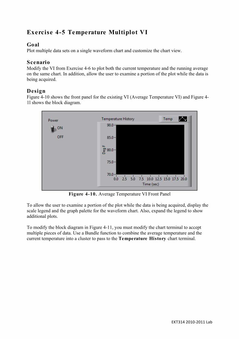
Exercise 4-5 Temperature Multiplot VI Goal Plot multiple data sets on a single waveform chart and customize the chart view. Scenario Modify the VI from Exercise 4-6 to plot both the current temperature and the running average on the same chart. In addition, allow the user to examine a portion of the plot while the data is being acquired. Design Figure 4-10 shows the front panel for the existing VI (Average Temperature VI) and Figure 4-1l shows the block diagram.

Figure 4-10. Average Temperature VI Front Panel

To allow the user to examine a portion of the plot while the data is being acquired, display the scale legend and the graph palette for the waveform chart. Also, expand the legend to show additional plots. To modify the block diagram in Figure 4-11, you must modify the chart terminal to accept multiple pieces of data. Use a Bundle function to combine the average temperature and the current temperature into a cluster to pass to the Temperature History chart terminal.

EKT3142010‐2011Lab

Figure 4-11. Average Temperature VI Block Diagram

Implementation 1. Open the Average Temperature VI you created in Exercise 4-4. If you have hardware, follow the instructions in the Hardware Installed column. Otherwise, follow the instructions in the No Hardware Installed column. Hardware Installed No Hardware Installed Open Average Temperature VI in the <Your_Drive>\Exercises\Average Temperature directory.

Open Average Temperature VI in the <Your_Drive>\Exercises\No Hardware Required\Average Temperature directory.

Select File»Save As and rename the VI Temperature Multiplot.vi in the <Your_Drive>\Exercises\Temperature Multiplot directory.

Select File»Save As and rename the VI Temperature Multiplot.vi in the <Your_Drive>\Exercises\No Hardware Required\Temperature Multiplot directory.

Tip Select the Substitute Copy for Original option to close the Average Temperature

VI and work in the Temperature Multiplot VI. You can create the directory if it does not exist.

EKT3142010‐2011Lab

In the following steps, you modify the block diagram so that it resembles Figure 4-12. Modify the block diagram Hrst, then modify the front panel.

Figure 4-12. Temperature Multiplot VI Block Diagram

2. Open the block diagram. 3. Pass the current temperature and the average temperature to the Temperature History chart terminal.

• Delete the wire connecting the Divide function to the Temperature History chart terminal.

• Add a Bundle function between the Divide function and the Temperature History chart indicator. lf necessary, enlarge the While Loop to make space.

• Wire the output of the Divide function to the top input of the Bundle function. • Wire the current temperature to the bottom input of the Bundle function. The current

temperature is the output of the Thermometer subVI inside the While Loop. • Wire the output of the Bundle function to the Temperature History chart indicator.

EKT3142010‐2011Lab

In the following steps, modify the front panel similar to the one shown in Figure 4-13.

Figure 4-13. Temperature Multiplot VI Front Panel

4. Open the front panel. 5. Show both plots in the plot legend of the waveform chart.

• Use the Positioning tool to resize the plot legend to two objects, using the top middle resizing node.

• Rename the top plot Running Avg. • Rename the bottom plot Current Temp. • Change the plot type of Current Temp. Use the Operating tool to select the plot in the

plot legend and choose the plots you want. Tip The order of the plots listed in the plot legend is the same as the order of the items wired to the Bundle function on the block diagram. 6. Show the scale legend and graph palette of the waveform chart.

• Right-click the Temperature History waveform chart and select Visible Items»Scale Legend from the shortcut menu.

• Right-click the Temperature History waveform chart and select Visible Items»Graph Palette from the shortcut menu.

7. Save the VI.

EKT3142010‐2011Lab

Test 1. Run the VI. Use the tools in the scale legend and the graph palette to examine the data as it generates. 2. Change the Power switch to the Off position to stop the VI. 3. Close the VI when you are finished. End of Exercise 4-5

EKT3142010‐2011Lab

Exercise 4-6 Determine Warnings VI Goal Modify a VI to use a Case structure to make a software decision. Scenario You created a VI where a user inputs a temperature, a maximum temperature, and a minimum temperature. A warning string generates depending on the relationship of the given inputs. However, a situation could occur that causes the VI to work incorrectly. The user could enter a maximum temperature that is less than the minimum temperature. Modify the VI to generate a different string to alert the user to the error: Upper Limit < Lower Limit. Set the Warning? indicator to True to indicate the error. Design Modify the flowchart created for the original Determine Warnings VI as shown in Figure 4-14.

Figure 4-14. Modified Determine Warnings Flowchart

EKT3142010‐2011Lab

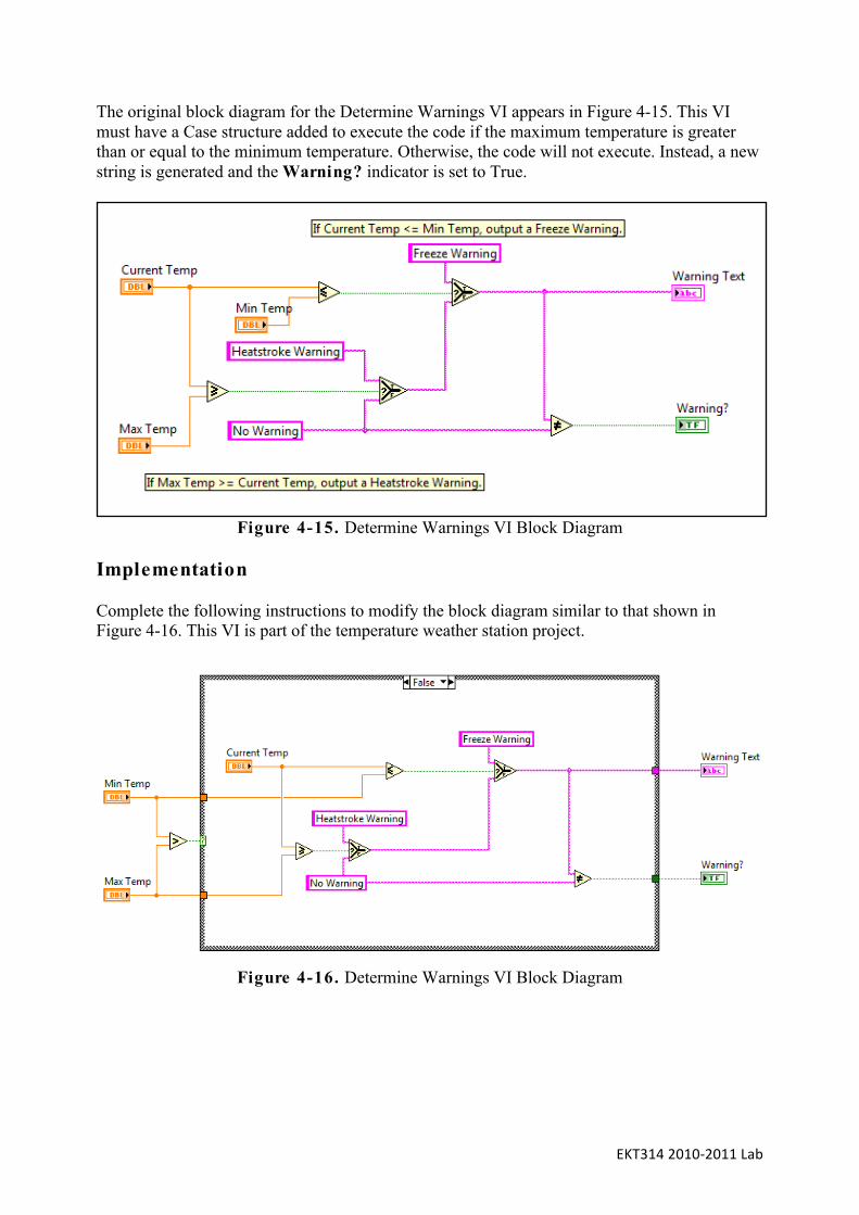
The original block diagram for the Determine Warnings VI appears in Figure 4-15. This VI must have a Case structure added to execute the code if the maximum temperature is greater than or equal to the minimum temperature. Otherwise, the code will not execute. Instead, a new string is generated and the Warning? indicator is set to True.

Figure 4-15. Determine Warnings VI Block Diagram

Implementation Complete the following instructions to modify the block diagram similar to that shown in Figure 4-16. This VI is part of the temperature weather station project.

Figure 4-16. Determine Warnings VI Block Diagram

EKT3142010‐2011Lab

1. Open the Determine Warnings VI in the <Your_Drive>\Exexcises>\Determine Warnings directory. You created the Determine Warnings VI in Exercise 4-l. 2. Open the block diagram. 3. Create space on the block diagram to add the Case structure. The Max Temp and Min Temp controls and the Warning Text and Warning? indicators should be outside of the new Case structure, because both cases of the Case structure use these indicators and controls.

• Select the Min Temp and Max Temp control terminals. Tip To select more than one item press the <Shift> key while you select the items.

• While the terminals are still selected, use the left arrow key on the keyboard to move the controls to the left.

Tip Press and hold the <Shift> key to move the objects in five pixel increments.

• Select the Warning Text and Warning? indicator terminals. • Align the terminals by selecting Align Objects»Left Edges . • While the terminals are still selected, use the right arrow key on the keyboard to move

the indicators to the right. 4. Compare Min Temp and Max Temp.

• Add the Greater? function to the block diagram. • Wire the Min Temp output to the x input of the Greater? function. • Wire the Max Temp output to the y input of the Greater? function. • Add a Case structure around the block diagram code, except for the excluded terminals. • Wire the output of the Greater? function to the case selector of the Case structure.

EKT3142010‐2011Lab

5. If Min Temp is less than Max Temp, execute the code that determines the warning string and indicator.

• While the True case is visible, right-click the border of the Case structure, and select Make This Case False from the shortcut menu. When you create a Case structure around existing code, the code is automatically placed in the True case.

6. If Min Temp is greater than Max Temp, create a custom string for the Warning Text indicator and set the Warning? indicator to True, as shown in Figure 4-l7.

Figure 4-17. Determine Warnings VI Block Diagram

• Select the True case. • Right-click the string output tunnel. • Select Create»Constant. • Enter Upper Limit < Lower Limit in the constant. • Right-click the Warning? output tunnel. • Select Create»Constant. • Use the Operating tool to change the constant to a True constant.

7. Save the VI.

EKT3142010‐2011Lab

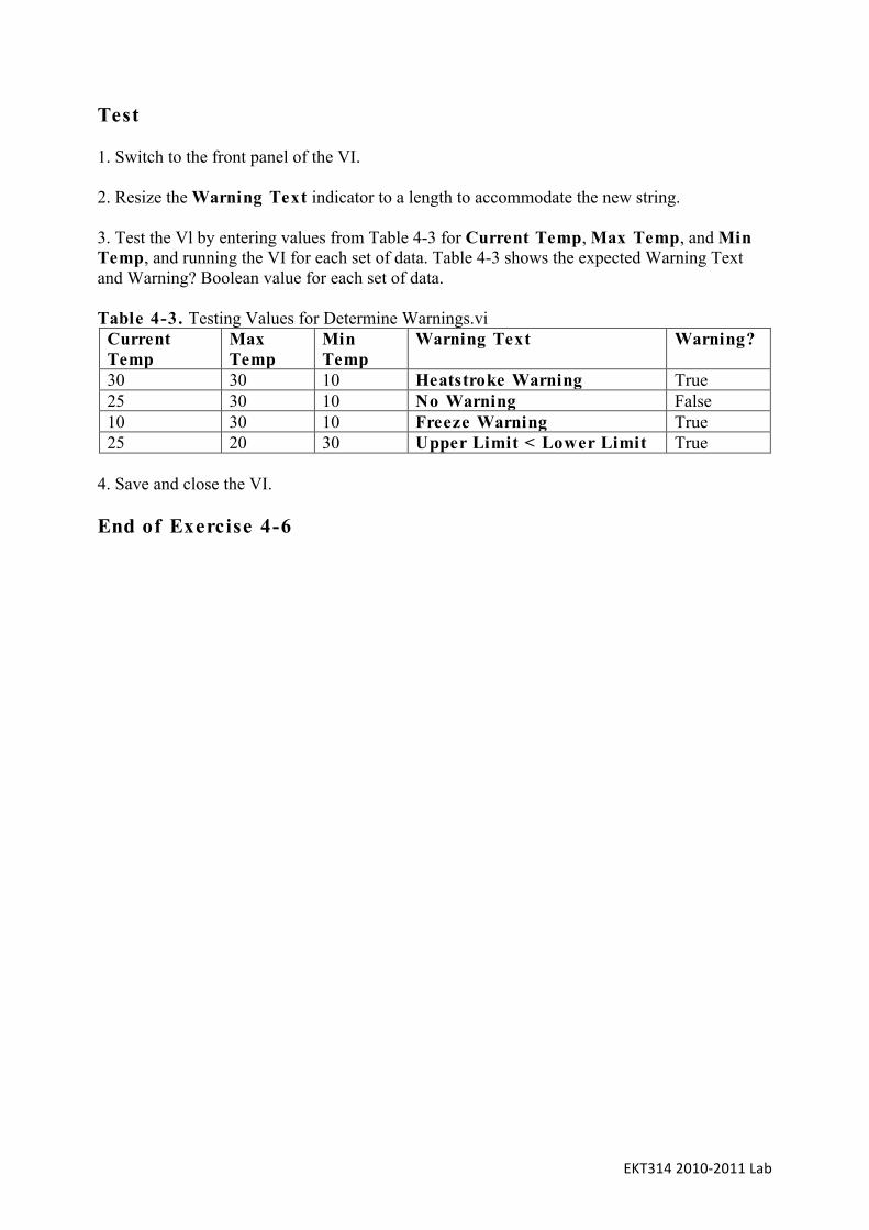
Test 1. Switch to the front panel of the VI. 2. Resize the Warning Text indicator to a length to accommodate the new string. 3. Test the Vl by entering values from Table 4-3 for Current Temp, Max Temp, and Min Temp, and running the VI for each set of data. Table 4-3 shows the expected Warning Text and Warning? Boolean value for each set of data. Table 4-3. Testing Values for Determine Warnings.vi

Current Temp

Max Temp

Min Temp

Warning Text Warning?

30 30 10 Heatstroke Warning True 25 30 10 No Warning False 10 30 10 Freeze Warning True 25 20 30 Upper Limit < Lower Limit True

4. Save and close the VI. End of Exercise 4-6

EKT3142010‐2011Lab

Exercise 4-7 Self-Study: Square Rect VI Goal Create a VI that uses a Case structure to make a software decision. Scenario Create a VI that calculates the square root of a number the user enters. If the number is negative, display the following message to the user: Error...Negative Number. Design Inputs and Outputs

Table 4-4. Inputs and Outputs Type Name Properties Input Number Double-precision, floating point;

default value of 25 Output Square Root Value Double-precision, floating point Flowchart

Figure 4-18. Square Root VI Flowchart

EKT3142010‐2011Lab

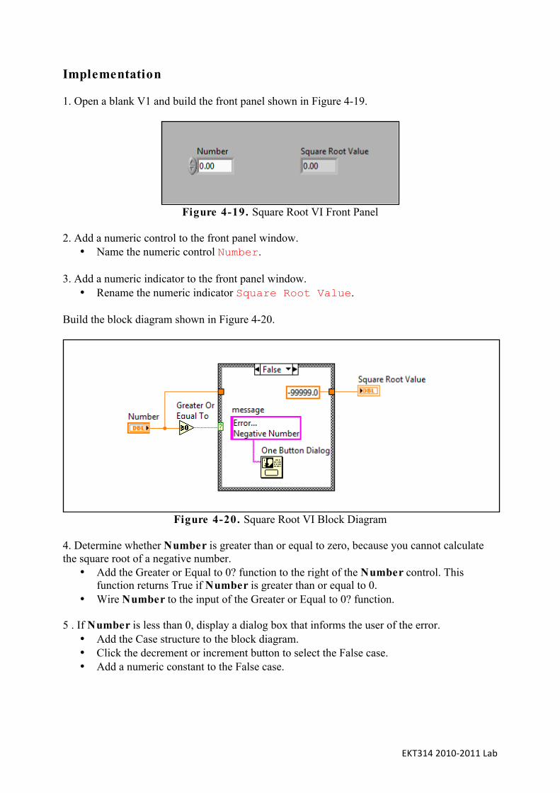
Implementation 1. Open a blank V1 and build the front panel shown in Figure 4-19.

Figure 4-19. Square Root VI Front Panel

2. Add a numeric control to the front panel window.

• Name the numeric control Number. 3. Add a numeric indicator to the front panel window.

• Rename the numeric indicator Square Root Value.

Build the block diagram shown in Figure 4-20.

Figure 4-20. Square Root VI Block Diagram

4. Determine whether Number is greater than or equal to zero, because you cannot calculate the square root of a negative number.

• Add the Greater or Equal to 0? function to the right of the Number control. This function returns True if Number is greater than or equal to 0.

• Wire Number to the input of the Greater or Equal to 0? function. 5 . If Number is less than 0, display a dialog box that informs the user of the error.

• Add the Case structure to the block diagram. • Click the decrement or increment button to select the False case. • Add a numeric constant to the False case.

EKT3142010‐2011Lab

• Right-click the numeric constant and select Representation»DBL. • Enter -99999 in the numeric constant. • Wire the numeric constant to the right edge of the Case structure. • Wire the new tunnel to the Square Root Value indicator. • Add the One Button Dialog function to the False case. This function displays a dialog

box that contains a message you specify. • Right-click the message input of the One Button Dialog function and select

Create»Constant from the shortcut menu. • Enter Error...Negative Number in the Constant. • Finish wiring the False case as shown in Figure 4-20.

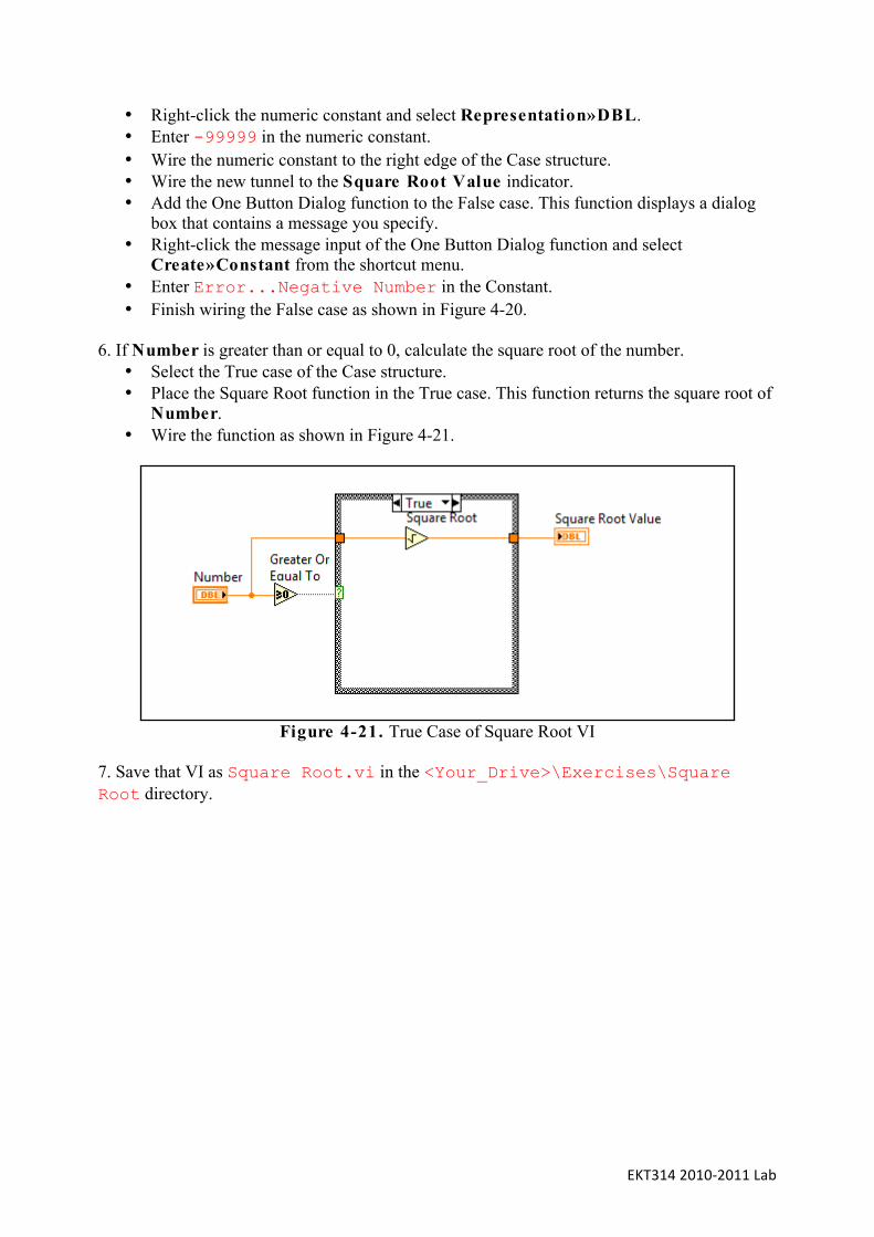
6. If Number is greater than or equal to 0, calculate the square root of the number.

• Select the True case of the Case structure. • Place the Square Root function in the True case. This function returns the square root of

Number. • Wire the function as shown in Figure 4-21.

Figure 4-21. True Case of Square Root VI

7. Save that VI as Square Root.vi in the <Your_Drive>\Exercises\Square Root directory.

EKT3142010‐2011Lab

Test 1. Display the front panel. 2. Enter a positive number in the Number control. 3. Run the VI. 4. Enter a negative number in the Number control. Caution Do not run this VI continuously. Under certain circumstances, continuously running this VI could result in an endless loop. 5. Run the VI.

If Number is positive, the VI executes the True case and returns the square root of Number. If Number is negative, the VI executes the False case, returns -99999, and displays a dialog box with the message Error...Negative Number.

6. Close the VI. End of Exercise 4-7

EKT3142010‐2011Lab

Exercise 4-8 Self-Study: Determine Warnings Vl (Challenge) Goal Modify an existing VI to use the Formula Node or a Case structure to make a software decision. Scenario In the Determine Warnings VI from Exercise 4-2, you used the Select function to pass a string based on a decision. Revise this block diagram to use either a Formula Node or a Case structure (or a combination of both) to complete the same purpose. Design Inputs and Outputs

Table 4-5. Determine Warnings VI Inputs and Outputs Type Name Properties Numeric Control Current Temp Double-precision,

f1oating-point Numeric Control Max Temp Double-precision,

floating-point Numeric Control Min Temp Double-precision,

Floating-point String Indicator Warning Text Three potential values:

Heatstroke Warning, No Warning, Or Freeze Warning

Round LED Warning? -

EKT3142010‐2011Lab

Flowchart Figure 4-22 shows the flowchart you used in Exercise 4-2 to create the Determine Warnings VI.

Figure 4-22. Determine Warnings VI Flowchart

EKT3142010‐2011Lab

Implementation As part of the challenge, no implementation instructions are given for this exercise. Start from the VI located in the <Your_Drive>\Exercises\Determine Warnings Challenge directory. End of Exercise 4-8

EKT3142010‐2011Lab

Exercise 4-9 Self-Study: Determine More Warnings VI Goal Manipulate strings using String functions. Scenario You have a VI that determines whether a Heatstroke Warning or a Freeze Warning has occurred, based on temperature input. You must expand this VI so that it also determines whether a High Wind Warning has occurred based on a wind speed reading and a maximum wind speed setting. The warnings must be displayed as a single string. For example, if a Heatstroke Warning and a High Wind Warning has occurred, the string should read: Heatstroke and High Wind Warning. Design Inputs and Outputs

Table 4-6. Determine More Warnings Vi Inputs and Outputs Type Name Properties Numeric Control Current Temp Double-precision, floating-point Numeric Control Max Temp Double-precision, floating-point Numeric Control Min Temp Double-precision, floating-point Numeric Control Current Wind

Speed Double-precision,floating-point

Numeric Control Max Wind Speed Double-precision, floating-point String Indicator Warning Text Potential values: Heatstroke Warning,

Freeze Warning, Heatstroke and High Wind Warning, Freeze and High Wind Warning, High Wind Warning and No Warning

Boolean Indicator Warning? Boolean

EKT3142010‐2011Lab

Flowchart The flowchart shown in Figure 4-23 is used for the Determine Warnings VI. This VI does not take wind data. Modify this flowchart to determine the High Wind Warning as well.

Figure 4-23. Determine Warnings VI Flowchart

EKT3142010‐2011Lab

The modified flowchart shown in Figure 4-24 determines the High Wind Warning in addition to the warnings already determined.

Figure 4-24. Determine More Warnings VI Flowchart

VI Architecture There are many ways to write this VI. In this exercise, you use Case structures to determine what string to pass, and the Concatenate Strings function to merge strings together.

EKT3142010‐2011Lab

Implementation A portion of this VI has already been built for you. The front panel of the VI is shown in Figure 4-25. This front panel retrieves values from the user for the current temperature, the maximum temperature, the minimum temperature, the current wind speed, and the maximum wind speed and displays to the user the warning string and the warning LED. The Weather Station project in this course does not use this VI.

Figure 4-25. Determine More Warnings Front Panel

1. Open the Determine More Warnings.vi in the <Your_Drive>\Exercises\Determine More Warnings directory. Create a block diagram similar to Figure 4-26. 2. Open the block diagram. 3. Use Figures 4-26 through 4-30 to assist you in building the block diagram code. 4. You use the following block diagram objects in this exercise:

• Case structure. • Empty String constant. • Space constant. • Equal? function. • Concatenate Strings function.

EKT3142010‐2011Lab

Figure 4-26. Determine More Warnings Block Diagram

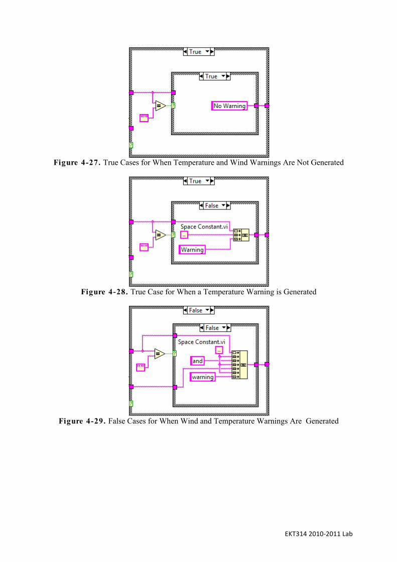
EKT3142010‐2011Lab

Figure 4-27. True Cases for When Temperature and Wind Warnings Are Not Generated

Figure 4-28. True Case for When a Temperature Warning is Generated

Figure 4-29. False Cases for When Wind and Temperature Warnings Are Generated

EKT3142010‐2011Lab

Figure 4-30. False Case for When a Wind Warning is Generated

5. Save the VI. Test 1. Test the following values to be sure your VI works as expected.

Table 4-7. Weather Test Values Name Test 1 Test 2 Test 3 Test 4 Test 5 Test 6 Currrent Temp 20 30 10 30 10 20 Max Temp 25 25 25 25 25 25 Min Temp 15 15 15 15 15 15 Current Wind Speed

25 25 25 35 35 35

Max Wind Speed

30 30 30 30 30 30

Warning Text No Warning

Heatstroke Warning

Freeze Warning

Heatstroke and High Wind Warning

Freeze and High Wind Warning

High Wind Warning

Warning? False True True True True True 2. Close and save the VI when you are finished. End of Exercise 4-9

EKT3142010‐2011Lab

Lesson 5: Relating Data Exercise 5-1 Concept: Manipulating Arrays Goal Manipulate arrays using various LabVIEW functions. Description You are given a VI and asked to enhance it for a variety of purposes. For each part of this exercise, begin with the Array Investigation.vi located in the <Your_Drive>\Exercises\Manipulating Arrays directory. The front panel of this VI is shown in Figure 5-1.

Figure 5-1. Array Investigation VI Front Panel

Figure 5-2 shows the block diagram of this VI.

Figure 5-2. Array Investigation VI Block Diagram

EKT3142010‐2011Lab

This exercise is divided into three parts. You are given the scenario for each part first. Refer to the end of this exercise for detailed implementation instructions for each part. Part 1: Iterate, Modify, and Graph Array Modify the Array Investigation VI so that after the array is created, the array is indexed into For Loops where you multiply each element of the array by 100 and coerce each element to the nearest whole number. Graph the resulting 2D array to an intensity graph. Part 2: Simplified Iterate, Modify, and Graph Array Modify the Array Investigation VI or the solution from Part 1 to accomplish the same goals without using the nested For Loops. Part 3: Create Subset Arrays Modify the Array Investigation VI so that the VI creates a new array that contains the contents of the third row, and another new array that contains the contents of the second column. Part 1: Implementation Modify the Array Investigation VI so that after the array is created, the array is indexed into For Loops where you multiply each element of the array by 100 and coerce each element to the nearest whole number. Graph the resulting 2D array on an intensity graph. 1. Open Array Investigation.vi located in the <Your_Drive>\Exercises\Manipulating Arrays directory. 2. Save the VI as Array Investigation Part I.vi. 3. Add an intensity graph to the front panel of the VI and autcscale the X and Y axes, as shown in Figure 5-3. To verify that autoscaling is enabled for the axes, right-click the intensity graph and select X Scale»AutoScale X and Y Scale»AutoScale Y and ensure these items are checked.

EKT3142010‐2011Lab

Figure 5-3. Array Investigation Part VI Front Panel

4. Open the block diagram of the VI. ln the following steps, you create a block diagram similar to Figure 5-4.

Figure 5-4. Array Investigation Part 1 VI Block Diagram

5. Iterate the Array.

• Add a For Loop to the right of the existing code. • Add a second For Loop inside the First For Loop. • Wire the array indicator terminal to the interior For Loop border. This creates an auto-

indexed input tunnel on both For Loops.

EKT3142010‐2011Lab

6. Multiply each element of the array by 100. • Add a Multiply function to the interior For Loop. • Wire the indexed input tunnel to the x input of the Multiply function. • Right-click the y input and select Create»Constant from the shortcut menu. • Enter 100 in the constant.

7. Round each element to the nearest whole number.

• Add a Round To Nearest function to the right of the Multiple function. • Wire the output of the Multiply function to the input of the Round To Nearest function.

8. Create a 2D array on the output of the For Loops to recreate the modified array.

• Wire the output of the Round To Nearest function to the outer For Loop. This creates an auto-indexed output tunnel on both For Loops.

9. Wire the output array to the Intensity Graph indicator. 10. Switch to the front panel. 11. Save the VI. 12. Enter values for Rows and Columns . 13. Run the Vl. Part 2: Implementation Modify Part 1 to accomplish the same goals without using the nested For Loops. 1. Open Array Investigation Part 1.vi if it is not still open. 2. Save the VI as Array Investigation Part 2.vi. 3. Open the block diagram. 4. Right-click the border of the interior For Loop, containing the Multiply function and the Round to Nearest function, and select Remove For Loop.

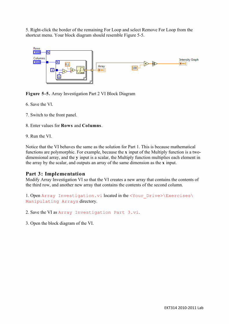
EKT3142010‐2011Lab

5. Right-click the border of the remaining For Loop and select Remove For Loop from the shortcut menu. Your block diagram should resemble Figure 5-5.

Figure 5-5. Array Investigation Part 2 VI Block Diagram 6. Save the Vl. 7. Switch to the front panel. 8. Enter values for Rows and Columns . 9. Run the VI. Notice that the VI behaves the same as the solution for Part 1. This is because mathematical functions are polymorphic. For example, because the x input of the Multiply function is a two-dimensional array, and the y input is a scalar, the Multiply function multiplies each element in the array by the scalar, and outputs an array of the same dimension as the x input. Part 3: Implementation Modify Array Investigation VI so that the VI creates a new array that contains the contents of the third row, and another new array that contains the contents of the second column. 1. Open Array Investigation.vi located in the <Your_Drive>\Exercises\ Manipulating Arrays directory. 2. Save the VI as Array Investigation Part 3.vi. 3. Open the block diagram of the VI.

EKT3142010‐2011Lab

In the following stops, you build a block diagram similar to that shown in Figure 5-6.

Figure 5-6. Array Investigation Part 3 VI Block Diagram

4. Retrieve the third row of data from Array using the Index Array function.

• Delete the items to the right of the Array indicator. • Add the Index Array function to the block diagram. • Wire Array to the array input of the Index Array function.

Tip The Index Array function accepts an n-dimensional array. After you wire the input array

to the Index Array function, the input and output terminal names change to match the dimension of the array wired. Therefore, wire the input array to the Index Array function before wiring any other terminals.

• Right-click the index(row) input of the Index Array function. • Select Create»Constant from the shortcut menu. • Enter 2 in the constant to retrieve the third row. Remember that the index begins at zero. • Right-click the subarray output of the Index Array function. • Select Create»Indicator from the shortcut menu. • Name the indicator Third Row.

EKT3142010‐2011Lab

5. Retrieve the second column of data from the Array using the Index Array function. • Add another Index Array function to the block diagram. • Wire Array to the array input of the Index Array function. • Right-click the disabled index(col) input of the Index Array function. • Select Create»Constant. • Enter 1 in the constant to retrieve the second column because the index begins at zero. • Right-click the subarray output of the Index Array function. • Select Create»Indicator. • Name the indicator Second Column.

6. Save the VI. 7. Switch to the front panel. 8. Enter values for Rows and Columns . 9. Run the VI. End of Exercise 5-1

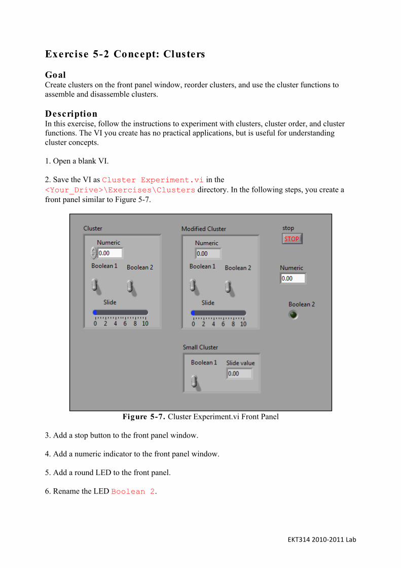
EKT3142010‐2011Lab

Exercise 5-2 Concept: Clusters Goal Create clusters on the front panel window, reorder clusters, and use the cluster functions to assemble and disassemble clusters. Description In this exercise, follow the instructions to experiment with clusters, cluster order, and cluster functions. The VI you create has no practical applications, but is useful for understanding cluster concepts. 1. Open a blank VI. 2. Save the VI as Cluster Experiment.vi in the <Your_Drive>\Exercises\Clusters directory. In the following steps, you create a front panel similar to Figure 5-7.

Figure 5-7. Cluster Experiment.vi Front Panel

3. Add a stop button to the front panel window. 4. Add a numeric indicator to the front panel window. 5. Add a round LED to the front panel. 6. Rename the LED Boolean 2.

EKT3142010‐2011Lab

7. Create a cluster named Cluster, containing a numeric, two toggle switches, and a slide. • Add a cluster shell to the front panel. • Add a numeric control to the cluster. • Add two vertical toggle switches to the cluster. • Rename the Boolean toggle switches to Boolean l and Boolean 2. • Add a horizontal till slide to the cluster.

8. Create Modified Cluster, containing the same contents as Cluster, but indicators instead of controls.

• Create a copy of Cluster. • Relabel the Copy Modified Cluster. • Right-click the shell of Modified Cluster, and select Change to Indicator from

the shortcut menu. 9. Create Small Cluster, containing a Boolean indicator and a numeric indicator.

• Create a copy of Modified Cluster. • Relabel the copy Small Cluster. • Delete the second toggle switch. • Delete the horizontal till slide indicator. • Right-click Small Cluster and select Autosizing»Size to Fit. • Relabel the numeric indicator to Slide value. • Resize the cluster as needed.

EKT3142010‐2011Lab

10. Verify the cluster order of Cluster, Modified Cluster, and Small Cluster. • Right-click the boundary of Cluster and select Reorder Controls in Cluster from

the shortcut menu. • Confirm the cluster order shown in Figure 5-8. • Click the Confirm button on the toolbar to set the cluster order and exit the cluster

order edit mode. • Right-click the boundary of Modified Cluster and select Reorder Controls in

Cluster from the shortcut menu. • Confirm the cluster orders shown in Figure 5-8. Modified Cluster should have the

same cluster order as Cluster. • Click the Confirm button on the toolbar to set the cluster order and exit the cluster

order edit mode. • Right-click the boundary of Small Cluster and select Reorder Controls in

Cluster from the shortcut menu. Click the Confirm button on the toolbar to set the cluster order and exit the cluster order edit mode.

• Confirm the cluster orders shown in Figure 5-8.

Figure 5-8. Cluster Orders

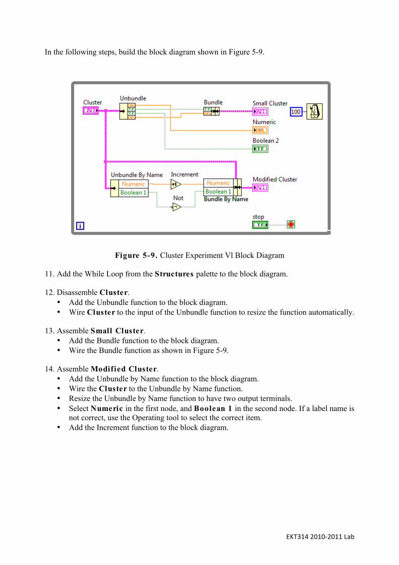
EKT3142010‐2011Lab

In the following steps, build the block diagram shown in Figure 5-9.

Figure 5-9. Cluster Experiment Vl Block Diagram

11. Add the While Loop from the Structures palette to the block diagram. 12. Disassemble Cluster.

• Add the Unbundle function to the block diagram. • Wire Cluster to the input of the Unbundle function to resize the function automatically.

13. Assemble Small Cluster.

• Add the Bundle function to the block diagram. • Wire the Bundle function as shown in Figure 5-9.

14. Assemble Modified Cluster.

• Add the Unbundle by Name function to the block diagram. • Wire the Cluster to the Unbundle by Name function. • Resize the Unbundle by Name function to have two output terminals. • Select Numeric in the first node, and Boolean 1 in the second node. If a label name is

not correct, use the Operating tool to select the correct item. • Add the Increment function to the block diagram.

EKT3142010‐2011Lab

• Wire the Numeric output of the Unbundle By Name function to the input of the Increment function. This function adds one to the value of Numeric .

• Add the Not function to the block diagram. • Wire the Boolean 1 output of the Unbundle By Name function to the x input of the

Not function. This function returns the logical opposite of the value of Boolean. • Add the Bundle by Name function to the block diagram. • Wire Cluster to the input cluster input. • Resize this function to have two input terminals. • Select Numeric in the first node and Boolean 1 in the second node. If a label name is

not correct, use the Operating tool to select the correct item. • Wire the output of the Increment function to Numeric. • Wire the output of the Not function to Boolean 1. • Wire the output of the Bundle By Name function to the Modified Cluster indicator.

15. Add a wait function to provide the processor with time to complete other tasks.

• Add the Wait Until Next ms Multiple function to the block diagram. • Right-click the millisecond multiple terminal of the Wait Until Next ms Multiple

function. • Select Create»Constant from the shortcut menu. • Enter 100 in the constant.

16. Complete the block diagram and wire the objects as shown in Figure 5-9. 17. Save the VI. 18. Display the front panel. 19. Run the VI.

EKT3142010‐2011Lab

20. Enter different values in Cluster and notice how values entered in Cluster affect the Modified Cluster and Small Cluster indicators. Is this the behavior you expected? 21. Click the Stop button when you are done. 22. Change the cluster order of Modified Cluster. Run the VI. How did the changed order affect the behavior? 23. Close the VI. Do not save changes. End of Exercise 5-2

EKT3142010‐2011Lab

Exercise 5-3 Concept: Type Definition Goal Explore the differences between a type definition and a strict type definition. Description l. Open a blank VI. 2. Create a custom control with a strict type definition status.

• Add a numeric control to the front panel window and rename it as Strict Type Def Numeric.

• Right-click the control and select Advanced»Customize from the shortcut menu to open the Control Editor.

• Select Strict Type Def. from the Control Type pull-down menu. • Right-click the numeric control and select Representation»Unsigned Long from

the shortcut menu. • Select File»Save . • Name the control Strict Type Def Numeric.ctl in the

<Your_Drive>\Exercises\Type Definition directory. • Close the Control Editor window. • Click Yes when asked if you would like to replace the original control.

3. Explore the strictly defined custom numeric.

• Right-click the Strict Type Def Numeric control and select Properties from the shortcut menu. Notice that the only options available are Appearance, Documentation, and Key Navigation. All other properties are defined by the strict type definition.

• Click Cancel to exit the Properties dialog box. • Right-click the Strict Type Def Numeric control again. Notice that representation is not

available on the shortcut menu. Also notice that you can open the type definition or disconnect from the type definition.

EKT3142010‐2011Lab

4. Edit the strict type def control. • Right-click the Strict Type Def Numeric control and select Open Type Def. from the

shortcut menu. • Right-click the numeric control and select Representation»DBL from the shortcut

menu in the Control Editor window. • Select File»Save . • Close the Control Editor window. • Select Help»Show Context Help to open the Context Help window. • Hover your mouse over the control on the VI and notice that it changed from a U32

numeric data type to a DBL numeric data type. • Right-click the Strict Type Def Numeric control and select Open Type Def. from the

shortcut menu. • Change the physical appearance of the numeric control by resizing it in the Control

Editor window. • Select File»Save . • Close the Control Editor window. • Notice that editing the strict type def control updates the size of the numeric control on

the VI front panel. 5. Create a custom control with a type definition status.

• Add another numeric control to the front panel window and rename it as Type Def Numeric.

• Right-click the control and select Advanced»Customize from the shortcut menu to open the Control Editor.

• Select Type Def. from the Control Type pull-down menu. • Right-click the numeric control and select Representation»Unsigned Long from

the shortcut menu. • Select File»Save . • Name the control Type Def Numeric.ctl in the

<Your_Drive>\Exercises\Type Definition directory.

EKT3142010‐2011Lab

• Close the Control Editor window. • Click Yes when asked if you would like to replace the original control.

6. Explore the type denned custom numeric.

• Right-click the Type Def Numeric control and select Properties from the shortcut menu. Notice that more items are available, such as Data Entry and Display Format.

• Click Cancel to exit the Properties dialog box. • Right-click the Type Def Numeric control again. Notice that Representation is

dimmed on the shortcut menu because the type definition defines the data type. Also notice that you can choose whether to auto-update with the type definition.

7. Edit the type def control.

• Right-click the Type Def Numeric control and select Open Type Def. from the shortcut menu.

• Right-click the Type Def Numeric control and select Representation»DBL from the shortcut menu in the Control Editor window.

• Select File»Save . • Close the Control Editor window. • Select Help»Show Context Help to open the Context Help window. • Hover your mouse over the Type Def Numeric control on the VI and notice that it

changed from a U32 numeric data type to a DBL numeric data type. • Right-click the Type Def Numeric control and select Open Type Def. from the

shortcut menu. • Change the physical appearance of the numeric control by resizing it in the Control

Editor window. • Select File»Save .

EKT3142010‐2011Lab

• Close the Control Editor window. • Notice that resizing the type def control in the Control Editor did not update the size of

the Type Def Numeric control on the VI front panel. Instances of a type def control will only update when the data type of the type definition changes.

8. Add another instance of the custom control to the front panel window and disconnect it from the type deinition.

• Select Select a Control from the Controls palette. • Select the Type Def Numeric.ctl from the

<Your_Drive>\Exercises\Type Definition directory. • Click OK. • Right-click the new control and select Disconnect from Type Def from the shortcut

menu. • Click OK. • Right-click the control again and notice that you can now change the Representation

because the numeric is no longer linked to the type definition. 9. Close the VI when you are finished. You do not need to save the VI. End of Exercise 5-3

EKT3142010‐2011Lab

Lesson 6: Managing Resources Exercise 6-1 Spreadsheet Example Vl Goal Save a 2D array in a text file so a spreadsheet application can access the file and to explore how to display numeric data in a table. Description Complete the following steps to examine a VI that saves numeric arrays to a file in a format you can access with a spreadsheet. l. Open the Spreadsheet Example VI located in the <Your_Drive>\Exercises\Spreadsheet Example directory. The following front panel window is already built.

Figure 6-1. Spreadsheet Example VI Front Panel

2. Run the VI. The VI generates a 2D array of 128 rows x 3 columns. The first column contains data for a sine waveform, the second column contains data for a noise waveform, and the third column contains data for a cosine waveform. The VI plots each column in a graph and displays the data in a table.

EKT3142010‐2011Lab

3. When the Choose file to write dialog box appears, save the tile as wave.txt in the <Your_Drive>\Exercises\Spreadsheet Example directory and click the OK button. Later, you will examine this file. 4. Display and examine the block diagram for this VI.

Figure 6-2. Spreadsheet Example VI Block Diagram

The Sine Pattern VI returns a numeric array of 128 elements containing a sine pattern. The constant 90.0, in the second instance of the Sine Pattern VI, specifies the phase of the sine pattern or cosine pattern. The Uniform White Noise VI returns a numeric array of 128 elements containing a noise pattern. The Build Array function builds the following 2D array from the sine array, noise array, and cosine array. Sine Array ... Noise Array ... Cosine Array ... The Transpose 2D Array function rearranges the elements of the 2D array so element [i,j] becomes element [j, i] , as follows. S N C

... ... ...

EKT3142010‐2011Lab

The Write To Spreadsheet File VI formats the 2D array into a spreadsheet string and writes the string to a file. The string has the following format, where an arrow (→) indicates a tab, and a paragraph symbol (¶) indicates an end of line character. S N C → →

¶

→ →

¶

→ →

¶

... ... ... → →

¶

The Number To Fractional String function converts an array of numeric values to an array of strings that the table displays. 5. Close the VI. Do not save changes. Note This example stores only three arrays in the file. To include more arrays, increase the

number of inputs to the Build Array function. 6. Open the wave.txt file using a word processor, spreadsheet application, or text editor and view its contents.

• Open a word processor, spreadsheet application, or text editor, such as Notepad or WordPad.

• Open wave.txt. The sine waveform data appear in the first column, the random waveform data appear in the second column, and the cosine waveform data appear in the third column.

7. Exit the word processor or spreadsheet application and return to LabVIEW. End of Exercise 6-1

EKT3142010‐2011Lab

Exercise 6-2 Temperature Log VI Goal Modify a VI to create an ASCII file using disk streaming. Description You have been given a VI that plots the current temperature and the average of the last three temperatures. Modify the VI to log the current temperature to an ASCII tile. Implementation 1. Open the exercise you created in Exercise 4-5. If you have hardware, follow the instructions in the Hardware Installed column. Otherwise, follow the instructions in the No Hardware Installed column.

Hardware Installed No Hardware Installed Open Temperature Multiplot.vi in the <Your_Drive>\Exercises\ Temperature Multiplot directory.

Open Temperature Multiplot.vi in the <Your_Drive>\Exercises\ No Hardware Required\Temperature Multiplot directory.

Select File»Save As and rename the VI as Temperature Log.vi in the <Your_Drive>\Exercises\ Temperature Log directory.

Select File»Save As and rename the VI as Temperature Log.vi in the <Your_Drive>\Exercises\ No Hardware Required\Temperature Log directory.

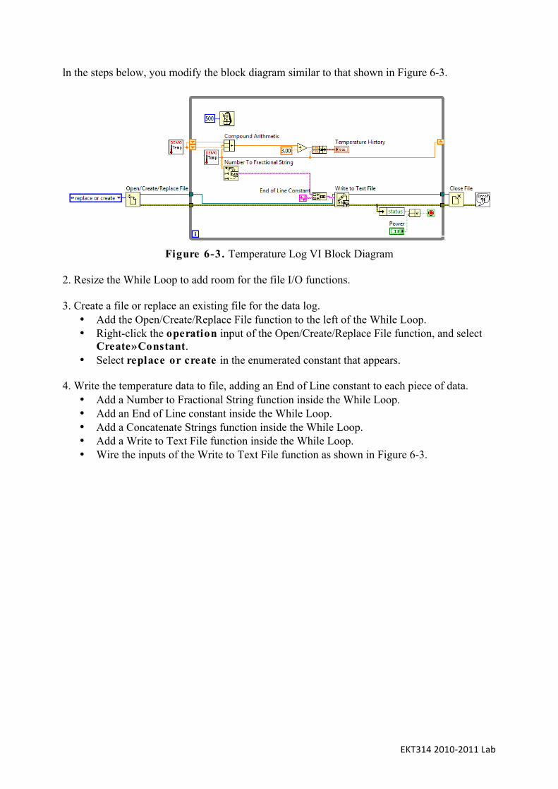
EKT3142010‐2011Lab

ln the steps below, you modify the block diagram similar to that shown in Figure 6-3.

Figure 6-3. Temperature Log VI Block Diagram

2. Resize the While Loop to add room for the file I/O functions. 3. Create a file or replace an existing file for the data log.

• Add the Open/Create/Replace File function to the left of the While Loop. • Right-click the operation input of the Open/Create/Replace File function, and select

Create»Constant. • Select replace or create in the enumerated constant that appears.

4. Write the temperature data to file, adding an End of Line constant to each piece of data.

• Add a Number to Fractional String function inside the While Loop. • Add an End of Line constant inside the While Loop. • Add a Concatenate Strings function inside the While Loop. • Add a Write to Text File function inside the While Loop. • Wire the inputs of the Write to Text File function as shown in Figure 6-3.

EKT3142010‐2011Lab

5. Stop the loop if an error occurs or if the user turns off the Power switch. • Delete the wire connecting the Power Boolean control to the conditional terminal. • Right-click the Loop Condition and select Stop if True . • Add a Compound Arithmetic function next to the conditional terminal.

o Right-click the Compound Arithmetic function and select Change Mode»OR. o Right-click the lower left input terminal of the Compound Arithmetic function

and select Invert. o Wire the Power control to the lower left input terminal of the Compound

Arithmetic function. • Add an Unbundle By Name function to the While Loop. • Wire the conditional terminal as shown in Figure 6-3.

6. Close the file and handle any errors that may have occurred.

• Add a Close File function to the right of the While Loop. • Add a Simple Error Handler VI to the right of the Close File function. • Finish wiring the block diagram as shown in Figure 6-3.

7. Save the VI. 8. Test the VI.

• Run the VI. • Give the text Hle a name and a location. • Turn the Power switch to Off after the VI has been running for a few samples. • Navigate to the text file created and explore it.

9. Close the VI and text file when you have finished. End of Exercise 6-2

EKT3142010‐2011Lab

Exercise 6-3 Using DAQmx

This exercise require hardware. Please ask your instructor for the device. Goal Explore a DAQmx example program that continuously acquires data, and modify it to wait on a digital trigger. Scenario Explore a DAQmx example program that continuously acquires a voltage signal on channel analog input l (AI1) of the DAQ device. Modify the VI to use a digital trigger. The VI begins measuring when a digital trigger is pressed and released. The VI stops measuring when the user clicks the stop button. Implementation External Connections l. Connect the sine function generator to channel All on the DAQ Signal Accessory with a wire. Open and run a DAQmx example 1. In LabVIEW, select Help»Find Examples to start the NI Example Finder. 2. Confirm that you are browsing according to task. 3. Navigate to Hardware Input and Output»DAQmx»Analog Measurements»Voltage in the task structure. 4. Double-click Cont Acq&Graph Voltage-Int Clk.vi to open the example program. This VI demonstrates how to acquire a continuous amount of data from a DAQ device. 5. Explore the block diagram.

• Go to the block diagram. • Press <Ctrl-H> to open the Context Help window. Hover over each of the DAQmx

functions to learn about each function. Read the steps listed in the comment to understand the functionality of the example program.

• Click the pull-down menu of the DAQmx Create Virtual Channel VI and notice that it is set to Analog Input»Voltage .

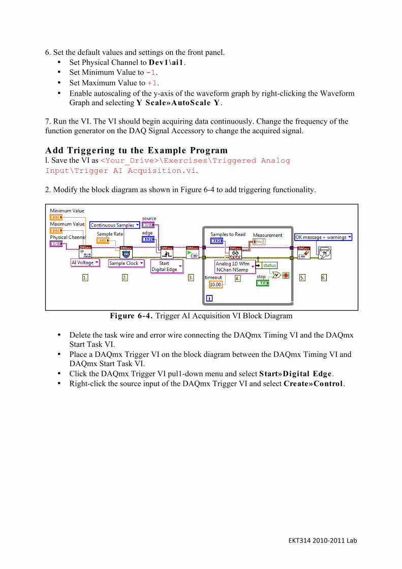
EKT3142010‐2011Lab

6. Set the default values and settings on the front panel. • Set Physical Channel to Dev1\ai1 . • Set Minimum Value to -1. • Set Maximum Value to +1. • Enable autoscaling of the y-axis of the waveform graph by right-clicking the Waveform

Graph and selecting Y Scale»AutoScale Y . 7. Run the VI. The VI should begin acquiring data continuously. Change the frequency of the function generator on the DAQ Signal Accessory to change the acquired signal. Add Triggering tu the Example Program l. Save the VI as <Your_Drive>\Exercises\Triggered Analog Input\Trigger AI Acquisition.vi. 2. Modify the block diagram as shown in Figure 6-4 to add triggering functionality.

Figure 6-4. Trigger AI Acquisition VI Block Diagram

• Delete the task wire and error wire connecting the DAQmx Timing VI and the DAQmx

Start Task VI. • Place a DAQmx Trigger VI on the block diagram between the DAQmx Timing VI and

DAQmx Start Task VI. • Click the DAQmx Trigger VI pul1-down menu and select Start»Digital Edge . • Right-click the source input of the DAQmx Trigger VI and select Create»Control .

EKT3142010‐2011Lab

• Right-click the edge input of the DAQmx Trigger VI and select Create»Control . • Connect the wires as shown in Figure 6-4.

3. Go to the front panel.

Figure 6-5. Trigger AI Acquisition VI Front Panel

4. Set source to PFI0 . 5. Set edge to Rising . 6. Save the VI. 7. Run the VI. Press and release the Digital Trigger button on the DAQ Signal Accessory to begin the acquisition. End of Exercise 6-3

EKT3142010‐2011Lab

Exercise 6-4 Concept: NI Devsim VI

Just read through and try what is possible. We do not have the simulator. Goal Install an instrument driver and explore the example programs that accompany the instrument driver. Description Install the instrument driver for the NI Instrument Simulator. After installation, explore the VIs that the instrument driver provides and the example programs that are added to the NI Example Finder. This lesson uses one of the following NI Instrument Simulators. Follow the instructions for the Instrument Simulator you are using.

Figure 6-6. NI Instrument Simulator A with DIP Switches

Figure 6-7. NI Instrument Simulator B Front Panel Select the exercise instructions that correspond to your instrument simulator.

• NI Instrument Simulator A, follow the instructions in Part A of this exercise. • NI Instrument Simulator B, follow the instructions in Part B of this exercise

EKT3142010‐2011Lab

Part A: NI Instrument Simulator A Install Instrument Driver 1. Exit LabVIEW. 2. Navigate to the <Your_Drive>\Exercises\Instrument Driver directory. This folder contains the LabVIEW Plug and Play instrument drivers for the Instrument Simulator. 3. Double-click the NI Instrument Simulator A Zip folder to extract the contents. 4. Extract to the <Program Files>\National Instruments\LabVIEW 2009\instr.lib directory. Explore Instrument Driver 1. Start LabVIEW. 2. Open a blank VI. 3. Switch to the block diagram. 4. Navigate to the NI Instrument Simulator category of the Functions palette. 5. Explore the palette using the Context Help window to familiarize yourself with the functionality. Use Example Programs 1. Select Help»Find Examples to start the NI Example Finder. 2. Confirm that you are browsing according to task. 3. Navigate to Hardware Input and Output»Instrument Drivers»LabVIEW Plug and Play in the task structure. 4. Double-click NI Instrument Simulator Read DMM Measurement.vi to open the example program. This VI reads a single measurement from the Instrument Simulator. 5. Prepare the Instrument Simulator. This VI can communicate with the instrument through serial or GPIB.

EKT3142010‐2011Lab

6. To communicate through serial, set the Instrument Simulator switches as shown in Figure 6-8. To apply the change, power cycle the Instrument Simulator.

Figure 6-8. Serial Configuration Settings for NI Instrument Simulator A 7. To communicate through GPIB, set the Instrument Simulator switches as shown in Figure 6-9. To apply the change, power cycle the Instrument Simulator.

Figure 6-9. GPIB Configuration Settings for NI instrument Simulator A 8. Select the communication type on the VISA Resource Name control.

• If you are using serial, select the resource (COM1 or COM2) that the serial cable is connected to.

• If you are using GPIB, select the devsim VISA alias. You specified the VISA alias for this GPIB instrument as devsim in Exercise 1-2.

9. Run the VI. 10. Explore the block diagram of the VI. Do not save changes. 11. Close the VI. 12. Return to the NI Example Finder.

EKT3142010‐2011Lab

13. Double-click NI Instrument Simulator Read Oscilloscope Waveform.vi to open the next example program. This VI reads a single waveform from the Instrument Simulator. 14. Select the same VISA Resource Name you selected in step 8. 15. Run the VI. 16. Choose a different Waveform Function. 17. Run the VI again. 18. Explore the block diagram of the VI.

• To familiarize yourself with the VI’s functionality, explore the block diagram using the Context Help window.

• Double-click the Read Waveform VI. • Go to the block diagram of the Read Waveform VI. • Doub1e-click the Write VI. • Go to the block diagram of the Write VI. Notice that it uses VISA functions to

communicate with the instrument. 19. Close the Vls and the NI Example Finder when you are finished. Do not save changes. Part B: NI Instrument Simulator B Install Instrument Driver 1. Exit LabVIEW. 2. Navigate to the <Your_Drive>\Exercises\Instruments Driver directory. This folder contains the LabVIEW Plug and Play instrument drivers for the Instrument Simulator. 3. Double-click the NI Instrument Simulator B Zip folder to extract the contents. 4. Extract to the <Program Files>\National Instruments\LabVIEW 2009\instr.lib directory.

EKT3142010‐2011Lab

Explore Instrument Driver 1. Start LabVIEW. 2. Open a blank VI. 3. Switch to the block diagram. 4. Navigate to the National Instruments Instrument Simulator category of the Functions palette. 5. Explore the palette using the Context Help window to familiarize yourself with the functionality. Use Example Programs 1. Select Help»Find Examples to start the NI Example Finder. 2. Confirm that you are browsing according to task. 3. Navigate to Hardware Input and Output»Instrument Drivers»LabVIEW Plug and Play in the task structure. 4. Double-click National Instruments Instrument Simulator Acquire Single Measurement(DMM).vi to open the example program. This VI reads a single measurement from the Instrument Simulator. 5. Verify that the PWR and RDY LEDs are lit on the NI Instrument Simulator. This VI can communicate with the instrument through serial or GPIB. 6. Select the communication type on the VISA Resource Name control.

• If you are using serial, select the resource (COM1 or COM2) that the serial cable is connected to.

• If you are using GPIB, select the devsim VISA alias. You specified the VISA alias for this GPIB instrument as devsim in Exercise 1-2.

7. Run the VI. 8. Explore the block diagram of the VI. Do not save changes. 9. Close the VI. 10. Return to the NI Example Finder. 11. Double-click National Instruments Instrument Simulator Acquire Waveform(Scope).vi to open the next example program. This VI reads a single waveform from the Instrument Simulator.

EKT3142010‐2011Lab

l2. Select the same VISA Resource Name you selected in step 8. 13. Run the VI. 14. Choose a different Waveform Function. 15. Run the VI again. 16. Explore the block diagram of the VI.

• To familiarize yourself with the VI’s functionality, explore the block diagram using the Context Help window.

• Double-click the Read Waveform VI. • Go to the block diagram of the Read Waveform VI. Notice that it uses VISA functions

to communicate with the instrument. l7. Close the Vls and the NI Example Finder when you are finished. Do not save changes. End of Exercise 6-4

EKT3142010‐2011Lab

Lesson 7: Developing Modular Applications Exercise 7-1 Determine Warnings VI Goal Create the icon and connector pane for a VI so that you can use the VI as a subVI. Scenario You have created a VI that determines a warning string based on the inputs given. Create an icon and a connector pane so that you can use this VI as a subVI. Design The subVI contains the following inputs and outputs:

Table 7-1. Determine Warnings SubVl Inputs and Outputs Inputs Outputs

Current Temp Warning Text Max Temp Warning? Min Temp - Use the standard connector pane to assure room for future expansion. Add error clusters to the VI so that the code runs if there is no error, but does not run if there is an error. Implementation l. Open the Determine Warnings VI in the <Your_Drive>\Exercises\Determine Warnings directory. YOu created the Determine Warnings VI in Exercise 4-1 and modified it in Exercise 4-6. 2. Add an error input cluster and an error output cluster to the VI.

• Add an Error In 3D.ctl to the front panel. • Add an Error Out 3D.ctl to the front panel.

EKT3142010‐2011Lab

3. Select a connector pane pattern for the VI. • Right-click the icon in the upper-right corner of the window and select Show

Connector from the shortcut menu. • Right-click the connector pane in the upper-right corner of the window, select Patterns

from the shortcut menu, and choose thepattern shown at left. 4. Connect the inputs and outputs to the connector as shown in Figure 7-1.

(1)Connections (2)ConnectorPane

Figure 7-1. Connector Pane Connections for Determine Warnings VI

• Using the wiring tool, click the upper-left terminal of the connector pane. • Click the corresponding front panel control, Current Temp.

Notice that the connector pane terminal fills in with a color to match the data type of the control connected to it.

• Click the next terminal in the connector pane. • Click the corresponding front panel control, Max Temp. • Continue wiring the connector pane until all controls and indicators are wired, and the

Context Help window matches that shown in Figure 7-1. 5. Create an icon.

• Right-click the connector pane and select Edit Icon. The Icon Editor window opens. • Use the tools in the Icon Editor window to create an icon. Make the icon as simple or as

complex as you want, however, it should be representative of the function of the Vl. Figure 7-2 shows a simple example of an icon for this VI.

EKT3142010‐2011Lab

Figure 7-2. Sample Warning lcon

6. Click OK when you are finished to close the Icon Editor window. Tip Double-click the selection tool to select the existing graphic. Press the <Delete> key to

delete the graphic. Then, double-click the rectangle tool to automatically create a border for the icon.

Tip Double-click the text tool to modify fonts. You can select Small Fonts to choose fonts

smaller than 9 points in size. Tip Select the Glyphs tab and filter the glyphs by the keyword warning. Then drag a

warning glyph onto your icon. 7. Right-click the connector pane and select Show Icon from the shortcut menu to return to Icon view. 8. Save the VI. 9. Switch to the block diagram.

EKT3142010‐2011Lab

10. Set the VI to execute if no error occurs, and not execute if an error occurs. • Surround the block diagram code with a Case structure as shown in Figure 7-3. Leave

the Warning Text and Warning? indictors outside of the Case structure.

Figure 7-3. No Error Case of Determine Warnings VI

• Wire the error in control to the case selector terminal. • Confirm that the block diagram is in the No Error case. lf it is not, switch to the case

containing the code, right-clicl< the Case structure and select Make this Case No Error from the shortcut menu.

• Wire the error cluster through the Case structure to the error out indicator as shown in Figure 7-3.

• Switch to the Error case. • Wire the error cluster through the case to the error out tunnel. • Right-click the Warning? tunnel and select Create»Constant from the shortcut menu. • Use the Operating tool to change the constant to True. • Right-click the Warning Text tunnel and select Create»Constant from the shortcut

menu. • Enter Error in the constant.

EKT3142010‐2011Lab

• Confirm that you have completed the Error case as shown in Figure 7-4.

Figure 7-4. Error Case of Determine Warnings VI

If an error enters the VI, the VI outputs Error in Warning Text, and True in Warning? and passes the error out of the VI. If an error does not enter the VI, the VI operates as originally designed. 11. Save and close the VI. Test Use a blank VI to test the subVI. l. Open a blank VI. 2. Open the block diagram. 3. Place the Determine Warnings subVI on the block diagram of the blank VI by selecting the Select a VI option on the Functions palette and navigating to the <Your_Drive>\Exercises\Determine Warnings directory. 4. Create controls and indicators for each item in the subVI.

• Right-click the Current Temp input and select Create»Control from the shortcut menu.

• Right-click the Max Temp input and select Create»Control from the shortcut menu.

EKT3142010‐2011Lab

• Right-click the Min Temp input and select Create»Control from the shortcut menu. • Right-click the Warning Text output and select Create»Indicator from the shortcut

menu. • Right-click the Warning? output and select Create»Indicator from the shortcut

menu. 5. Switch to the front panel. 6. Enter test values in Current Temp, Max Temp, and Min Temp. 7. Run the VI. 8. After you have finished testing, close the test VI. You do not need to save the test VI. End of Exercise 7-1

EKT3142010‐2011Lab

Lesson 8: Common Design Techniques and Patterns Exercise 8-1 State Machine VI Goal Create a VI that implements a state machine using a type-defined enum. Scenario You must design a template for a user interface state machine. The state machine must allow the user to activate Process l or Process 2 in any order. The state machine must also allow for expansion, because processes may be added in the future. Design Inputs and Outputs

Table 8-1. Inputs and Outputs Type Name Properties

Cancel Button Process 1 Boolean Text: Process 1 Cancel Button Process 2 Boolean Text: Process 2 Stop Button Stop - State Transitions

Table 8-2. Inputs and Outputs State Action Next State

Idle Poll user interface for selection

No button clicked: Idle State Process l clicked: Process 1 State Process 2 clicked: Process 2 State Stop clicked: Stop State

Process 1 Execute Process 1 code Idle State

EKT3142010‐2011Lab

Table 8-2. Inputs and Outputs (Continued)

State Action Next State Process 2 Execute Prccess 2

code Idle State

Stop Stop the state machine Stop State Implementation In the following steps, you will create the front panel window shown in Figure 8-l.

Figure 8-1. State Machine VI Front Panel Window

l. Create a new project containing a blank VI.

• Select Empty Project from the Getting Started window. • Select File»Save Project. • Name the project State Machine.lvproj in the

<Your_Drive>\Exercises\State Machine directory. • Select File»New VI. • Save the new VI as State Machine.vi in the

<Your_Drive>\Exercises\State Machine directory. 2. Create a menu cluster containing buttons for running process 1, running process 2, and stopping the VI.

• Place a cluster shell on the front panel window. • Relabel the cluster Menu. • Add a Cancel button to the cluster shell. • Relabel the Cancel button Process 1.

EKT3142010‐2011Lab

• Change the Boolean text Run Process l. • Make a copy of the Process l button, and place the copy within the cluster shell. • Rename the copied button Process 2. • Change the Boolean text on the copied button to Run Process 2. • Right-click each button and select Visible Items»Label to hide the labels. • Add a stop button to the cluster shell. • Right-click the Stop button and select Visible Items»Label to hide the label. • Modify the Boolean text on the buttons using the Text Settings on the toolbar. Suggested text settings: 24 point bold Application Font. • Enlarge and arrange the buttons within the cluster using the resizing tool and the

following toolbar buttons: Align Objects , Distribute Objects , and Resize Objects .

• Right-click the border of the cluster and select Autosizing»Size to Fit. • Right-click the border ofthe cluster and select Visible Items»Label to hide the label.

3. Create the type-deiined enum to control the state machine.

• Add an enum to the front panel window. • Right-click the enum and select Edit Items . Modify the list as follows:

Items Digital Display Idle 0 Process l l Process 2 2 Stop 3

EKT3142010‐2011Lab

• Select OK to exit the Enum Properties dialog box. • Relabel the enum control State Enum. • Right-click the State Enum and select Advanced»Customize . • Select Type Def. from the Control Type pull-down menu. • Right-click the Enum and select Representation»U32 . • Save the control as State Enum.ctl in the

<Your_Drive>\Exercises\State Machine directory. • Close the Control Editor window. • Click Yes when asked if you would like to replace the control. • Switch to the block diagram. • Right-click the State Enum and select Change to Constant. The enumerate control

no longer appears on the front panel window. In the following steps, you create the block diagram shown in Figure 8-2. This block diagram contains four states-Idle, Process l, Process 2, and Stop.

Figure 8-2. Idle State

4. Create the block diagram shown in Figure 8-2.

• Wire the enum to the Case structure using a shift register on the While Loop.

EKT3142010‐2011Lab

• After you wire the enumerated constant to the case selector terminal of the Case structure, right-click the Case structure and select Add Case for Every Value to automatically add a case for each item in the enum.

• Copy the enum to use within the Case structure. The copy is also linked to the type-defined enum.

• Wire a False constant to the conditional terminal; the state machine should not stop when exiting the Idle state.

• In the Idle state, you convert the cluster to an array so that the array • can be searched for any button clicked. The Search ID Array function returns the index

of the button clicked. Because the Idle State does not have a button associated with it, this index must be incremented by one. Use the Type Cast function to select the appropriate item from the enum constant. It is very important that the order of the cluster matches the order of the items in the enumerated constant.

5. Complete the Process l state shown in Figure 8-3.

Figure 8-3. Process 1 State

• Use a One Button Dialog function to simulate the Process l code. • Wire a False constant to the conditional terminal; the state machine should not stop

when exiting the Process l state.

EKT3142010‐2011Lab

6. Complete the Process 2 state shown in Figure 8-4.

Figure 8-4. Process 2 State

• Use a One Button Dialog function to simulate the Process 2 code. • Wire a False constant to the conditional terminal; the state machine should not stop

when exiting the Process 2 state. 7. Complete the Stop state shown in Figure 8-5.

Figure 8-5. Stop State

• Pass a True constant to the conditional terminal; the state machine should stop only

from this state. 8. Save the VI when you have finished.

EKT3142010‐2011Lab

Test l. Switch to the front panel window. 2. Run the VI. Experiment with the VI to be sure it works as expected. If it does not, compare your block diagram to Figures 8-2 through 8-5. 3. Save and close the VI when you are finished. End of Exercise 8-1

EKT3142010‐2011Lab

Lesson 9: Using Variables Exercise 9-1 Local Variable VI Goal Use a local variable to write to and read from a control Scenario You have a LabVIEW Project that implements a temperature weather station. The weather station acquires a temperature every half a second, analyzes each temperature to determine if the temperature is too high or too low, then alerts the user if there is a danger of a heat stroke or freeze. The VI logs the data if a warning occurs. Two front panel controls determine the setpoints – the temperature upper limit and the temperature lower limit. However, nothing prevents the user from setting a lower limit that is higher than the upper limit. Use a local variable to set the lower limit equal to the upper limit if the user sets a lower limit that is higher than the upper limit. Design The Vls in this project have already been written. Your only task is to modify the Vls so that the lower limit is set equal to the upper limit when necessary. State Definitions The following table describes the states in the state machine.

State Description Next State Acquisition Set time to zero, acquire data

from the temperature sensor, and read front panel controls

Analysis

Analysis Determine warning level Data Log if a warning cccurs, Time Check if no warning occurs

EKT3142010‐2011Lab

State Description Next State Data Log Log the data in a

tab-delimited ASCII file

Time Check

Time Check Check whether time is greater than or equal to .5 seconds

Acquisition if time has elapsed, Time Check if time has not elapsed

Changing the value of the lower temperature limit control should happen after the user has entered the value but before the value determines the warning level. Therefore, make the modifications to the VI in the Acquisition or Analysis state, or place a new state between the two. 1. Before determining which option to use, take a closer look at the content of the Acquisition and Analysis states:

• Open the Weather Station project located in the <Your_Drive>\Exercises\Variables directory.

• Open Weather Station UI.vi. • Review the contents of the Acquisition and Analysis states, which correspond to the

Acquisition and Analysis cases of the Case structure.

EKT3142010‐2011Lab

Design Options You have three different design options for modifying this project. Option Description Benefits/Drawbacks 1 Insert a Case structure in the

Acquisition state to reset the controls before a local variable writes the values to the cluster.

Poor design: the acquisition state has another task added, rather than focusing only on acquisition.

2 Insert a new state in the state machine that checks the controls and resets them if necessary.

Ability to control when the state occurs.

3 Modify the Determine Warnings subVI to reset the controls.

Easy to implement because functionality is already partially in place. However, if current functionality is used, one set of data always is lost when resetting the lower limit control.

This exercise implements Option 2 as a solution.

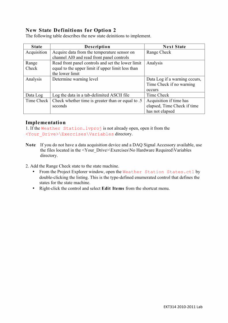
EKT3142010‐2011Lab

New State Definitions for Option 2 The following table describes the new state deinitions to implement.

State Description Next State Acquisition Acquire data from the temperature sensor on

channel AI0 and read front panel controls Range Check

Range Check

Read front panel controls and set the lower limit equal to the upper limit if upper limit less than the lower limit

Analysis

Analysis Determine warning level Data Log if a warning cccurs, Time Check if no warning occurs

Data Log Log the data in a tab-delimited ASCII file Time Check Time Check Check whether time is greater than or equal to .5

seconds Acquisition if time has elapsed, Time Check if time has not elapsed

Implementation 1. If the Weather Station.lvproj is not already open, open it from the <Your_Drive>\Exercises\Variables directory. Note If you do not have a data acquisition device and a DAQ Signal Accessory available, use

the files located in the <Your_Drive>\Exercises\No Hardware Required\Variables directory.

2. Add the Range Check state to the state machine.

• From the Project Explorer window, open the Weather Station States.ctl by double-clicking the listing. This is the type-defined enumerated control that defines the states for the state machine.

• Right-click the control and select Edit Items from the shortcut menu.

EKT3142010‐2011Lab

• Insert an item and modify to match Table 9-l. Be careful not to add an empty listing.

Table 9-1. States Enumerated Control Item Digital Display

Acquire 0 Range Check l Analysis 2 Data Log 3 Time Check 4

• Save and close the control. • If the Weather Station UI.vi is not open, open it by double-clicking the listing

in the Project Explorer window. • Open the block diagram. • Right-click the state machine Case structure and select Add Case for Every Value

from the shortcut menu. Because the enumerated control has a new value, a new case appears in the Case structure.

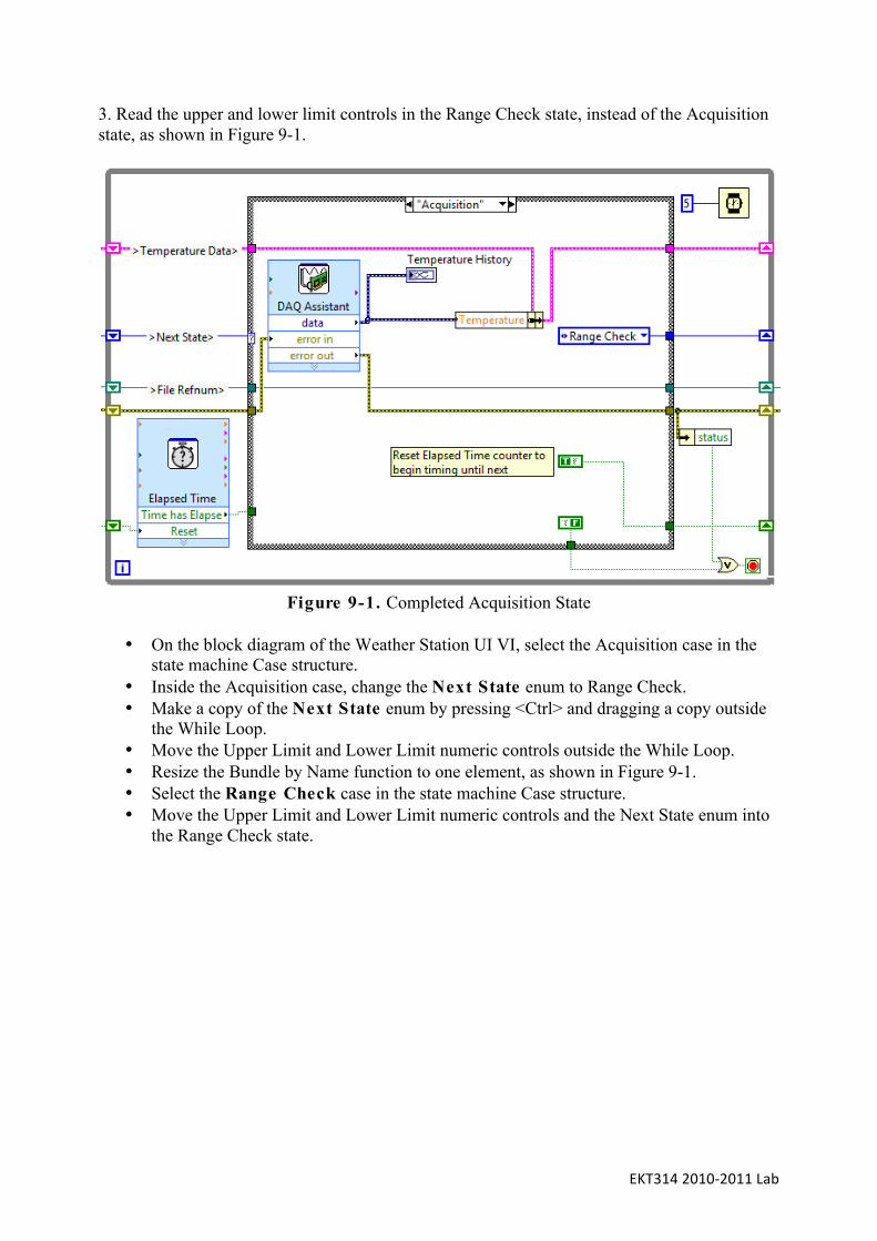
EKT3142010‐2011Lab

3. Read the upper and lower limit controls in the Range Check state, instead of the Acquisition state, as shown in Figure 9-1.

Figure 9-1. Completed Acquisition State

• On the block diagram of the Weather Station UI VI, select the Acquisition case in the

state machine Case structure. • Inside the Acquisition case, change the Next State enum to Range Check. • Make a copy of the Next State enum by pressing <Ctrl> and dragging a copy outside

the While Loop. • Move the Upper Limit and Lower Limit numeric controls outside the While Loop. • Resize the Bundle by Name function to one element, as shown in Figure 9-1. • Select the Range Check case in the state machine Case structure. • Move the Upper Limit and Lower Limit numeric controls and the Next State enum into

the Range Check state.

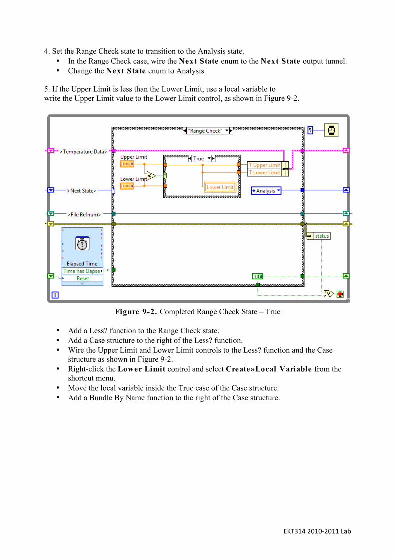
EKT3142010‐2011Lab

4. Set the Range Check state to transition to the Analysis state. • In the Range Check case, wire the Next State enum to the Next State output tunnel. • Change the Next State enum to Analysis.

5. If the Upper Limit is less than the Lower Limit, use a local variable to write the Upper Limit value to the Lower Limit control, as shown in Figure 9-2.

Figure 9-2. Completed Range Check State – True

• Add a Less? function to the Range Check state. • Add a Case structure to the right of the Less? function. • Wire the Upper Limit and Lower Limit controls to the Less? function and the Case

structure as shown in Figure 9-2. • Right-click the Lower Limit control and select Create»Local Variable from the

shortcut menu. • Move the local variable inside the True case of the Case structure. • Add a Bundle By Name function to the right of the Case structure.

EKT3142010‐2011Lab

• Wire the Temperature Data cluster to the input cluster input of the Bundle By Name function.

• Expand the Bundle By Name function to two elements. • Select T Upper Limit in the first element and T Lower Limit in the second element. • Add a False constant to the outer Case structure. • Wire the case as shown in Figure 9-2.

6. lf the Upper Limit is equal to or greater than the Lower Limit, pass the values of the controls to the temperature cluster, as shown in Figure 9-3.

Figure 9-3. Completed Range Check State – False

• Switch to the False case ofthe interior Case structure. • Wire the Upper Limit and Lower Limit data through the case.

7. Save the VI. 8. Save the Project.

EKT3142010‐2011Lab

Test l. Run the VI.

• Name the log file when prompted. • Enter a value in the Upper Limit control that is less than the value in the Lower

Limit control. Does the VI behave as expected? 2. Stop the VI when you are finished. 3. Close the VI and the project. End of Exercise 9-1

EKT3142010‐2011Lab

Exercise 9-2 Global Data Project Goal Create a project containing multiple Vls that share data using a single-process shared variable. Scenario Create a VI that generates a sine wave. Create a second VI that displays the sine wave and allows the user to modify the time between each acquisition of the sine wave data. Use one stop button to stop both Vls. Design Two VIs and two pieces of global data are necessary to implement the VI:

• First VI: generate sine, write sine to Data shared variable, read Stop shared variable to stop loop

• Second VI: read Data shared variable, display on chart, write Stop button to Stop shared variable

• First shared variable: Stop (Boolean data type) • Second shared variable: Data (Numeric data type)

Implementation l. Open an empty project. 2. Save the project as Global Data.lvproj in the <Your_Drive>\Exercises\Global Data directory. 3. Create the Stop shared variable.

• Give the variable the following properties. o Name: Stop o Variable Type: Single-process o Data Type: Boolean

• Click OK to close the Shared Variable Properties dialog box. Notice that a new library is created in the Project Explorer window to hold the variable.

EKT3142010‐2011Lab

4. Save the library. • Right-click the library and select Save from the shortcut menu. • Save the library as Global Data.lvlib in the

<Your_Drive>\Exercises\Global Data directory. 5. Create the Data shared variable.

• Switch to the Project Explorer window. • Right-click Global Data.lvlib and select New»Variable from the shortcut menu. • Give the new variable the following properties:

o Name: Data o Variable Type: Single-process o Data Type: Double

• Click OK to close the Shared Variable Properties dialog box. Generate Data VI l. Open a blank VI. 2. Save the VI as Generate Data.vi in the <Your_Drive>\Exercises\Global Data directory. 3. Add a Numeric Indicator to the front panel window. 4. Name the Numeric Indicator Data. 5. Switch to the block diagram of the VI.

EKT3142010‐2011Lab

6. Create the block diagram shown in Figure 9-4. No implementation instructions are given. Labels are shown to assist you.

Figure 9-4. Generate Data Block Diagram without Variables

7. Save the VI. 8. Write the data generated to the Data shared variable.

• Select the Data shared variable from the Project Explorer window and drag it inside the While Loop of the Generate Data VI block diagram.

• Right-click the global variable and select Change to Write from the shortcut menu. • Wire the Sin(x) output of the Sine function to the Data shared variable.

9. Read the Stop shared variable to stop the While Loop.

• Switch to the Project Explorer window. • Select the Stop shared variable and drag it inside the While Loop of the Generate

Data.vi block diagram. • Wire the Stop shared variable to the Loop Condition terminal.

l0. Initialize the Stop shared variable.

• Switch to the Project Explorer window. • Select the Stop shared variable and drag it to the left of the While Loop of the

Generate Data.vi block diagram. • Right-click the Stop shared variable and select Change to Write from the shortcut

menu.

EKT3142010‐2011Lab

• Right-click the input of the Stop shared variable and select Create»Constant from the shortcut menu to create a False constant.

• Use the Operating tool to change the constant to False if necessary. ll. Use the shared variable error clusters to ensure the order of operations. Refer to Figure 9-5 for assistance wiring this block diagram.

Figure 9-5. Generate Data Block Diagram with Shared Variables

12. Save the VI. 13. Close the block diagram, but leave the front panel open. Read Data VI 1. Open a blank VI. 2. Save the VI as Read Data.vi in the <Your_Drive>\Exercises\Global Data directory. 3. Create the front panel shown in Figure 9-6.

Figure 9-6. Read Data Front Panel

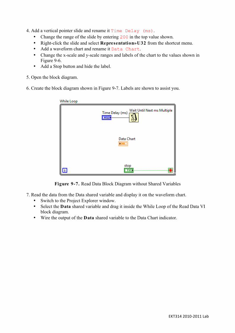
EKT3142010‐2011Lab

4. Add a vertical pointer slide and rename it Time Delay (ms). • Change the range of the slide by entering 200 in the top value shown. • Right-click the slide and select Representation»U32 from the shortcut menu. • Add a waveform chart and rename it Data Chart. • Change the x-scale and y-scale ranges and labels of the chart to the values shown in

Figure 9-6. • Add a Stop button and hide the label.

5. Open the block diagram. 6. Create the block diagram shown in Figure 9-7. Labels are shown to assist you.

Figure 9-7. Read Data Block Diagram without Shared Variables

7. Read the data from the Data shared variable and display it on the waveform chart.

• Switch to the Project Explorer window. • Select the Data shared variable and drag it inside the While Loop of the Read Data VI

block diagram. • Wire the output of the Data shared variable to the Data Chart indicator.

EKT3142010‐2011Lab

8. Write the value of the Stop control to the Stop shared variable. • Switch to the Project Explorer window. • Select the Stop shared variable and drag it inside the While Loop of the Read

Data.vi block diagram. • Right-click the Stop shared variable and select Change to Write from the shortcut

menu. • Wire the Stop control to the Stop shared variable.

9. Use the shared variable error clusters to ensure the order of operations. Refer to Figure 9-8 for assistance wiring this block diagram.

Figure 9-8. Read Data Block Diagram with Shared Variables

10. Save the VI. 11. Close the block diagram. 12. Save the project.

EKT3142010‐2011Lab

Test l. Run the Generate Data VI. 2. Run the Read Data VI. 3. Modify the value of the Time Delay (ms) control. The Time Delay (ms) control determines how often the shared variable i is read. What happens if you set the Time Delay to zero? When accessing global data, you may read the value more than once before it is updated to a new value, or you may miss a new value altogether, depending on the value of the Time Delay. 4. Stop and close the VIs and the project when you are finished. Challenge Create a functional global variable to handle the Stop data and use it in the Generate Data VI and the Read Data VI to share the stop button between the two VIs. End of Exercise 9-2

EKT3142010‐2011Lab

Exercise 9-3 Concept: Bank VI

Goal Eliminate a race condition in a VI. Description You must identify and fix a problem with the server software in a bank. The bank server handles requests from many sources and must process the requests quickly. In order to increase its efficiency, the server uses two parallel loops-one to handle deposits to the account and another to handle withdrawals. The problem with the server is that some deposit or withdrawal requests are lost, thereby resulting in incorrect balances. Identity Race Condition l. Open Bank.vi in the <Your_Drive>\Exercises\Bank directory. 2. Run the VI. 3. Perform a deposit, a withdrawal, and a simultaneous transaction to familiarize yourself with the program. 4. Set the Deposit Amount to 20 and the Withdrawal Amount to 10. 5. Open the block diagram of the Bank VI while it is still running. 6. Arrange the block diagram of the Bank VI so that you can see it while operating the user interface. 7. Enable execution highlighting on the block diagram by clicking Highlight Execution. 8. Click the Simultaneous Transactions button and watch the code as it executes. The balance should increase by 10. Notice that either the deposit or the withdrawal is lost, causing the balance to increase by 20 or decrease by l0. 9. Stop the VI. You tracked the problem down to a race condition in a section of a code handling deposits and withdrawals for a single account. Although you can see the issue with execution highlighting enabled, during regular operation, the issue would occur sporadically.

EKT3142010‐2011Lab

Remove Race Condition Remove the race condition by protecting the critical section of code using a semaphore. In the VI, the critical sections of code are those enclosed by a Sequence structure. l. Save the Bank VI as Bank with Semaphores.vi in the <Your_Drive>\Exercises\Bank directory. 2. Use semaphores to protect the critical sections of code, as shown in Figure 9-9.

Figure 9-9. Bank with Semaphore

• Add a Obtain Semaphore Reference VI to the left of the While Loops. • Wire the Obtain Semaphore Reference VI as shown in Figure 9-9. • Add an Acquire Semaphore VI to the Deposit Handler loop, to the left of the Sequence

structure. • Add a second Acquire Semaphore VI to the Withdrawal Handler loop to the left of the

Sequence structure. • Wire the Acquire Semaphore Vls as shown in Figure 9-9.

EKT3142010‐2011Lab

• Add a Release Semaphore VI to the Deposit Handler loop, to the right of the Sequence structure.

• Add a second Release Semaphore VI to the Withdrawal Handler loop, to the right of the Sequence structure.

• Wire the Release Semaphore Vls as shown in Figure 9-9. • Add a Release Semaphore Reference VI to the right of the While Loops. • Wire the Release Semaphore Reference VI as shown in Figure 9-9. Notice that the

Release Semaphore Reference VI requires only the • reference to the semaphore.

3. Save the VI. 4. Repeat the steps detailed in the Identify Race Condition section to test the modification to this VI. 5. Close the VI when you are finished. End of Exercise 9-3

EKT3142010‐2011Lab

Exercise A-1 Concept: Analysis Types Goal Choose when to use inline, offline, programmatic, or interactive analysis for an application. Description For each scenario, determine which form(s) of analysis to use. Most scenarios use more than one form. Scenario 1 The failure rate of your manufacturing line is related directly to the speed of production. You need to monitor the failure rate programmatically. If the failure rate is greater than 3%, decrease the speed of the line. lf the failure fate is less than 2%, increase the speed of the line. Inline Offline Programmatic Interactive Scenario 2 You are listening to a radio station. The frequency components of the radio station signal are determined and recorded to file. lf you have difficulty hearing the radio station, you tell the VI to pass the signal through a filter before recording the data. Inline Offline Programmatic Interactive Scenario 3 You are recording temperature and pressure data. Once a week, you prepare a report for your manager correlating the temperature and pressure trends during thunderstorms. Inline Offline Programmatic Interactive

EKT3142010‐2011Lab

Scenario 4 You are performing stress analysis on a bridge. During rush hour, you must also record vibration data on the bridge. It is considered rush hour when more than 100 cars use the bridge in 5 minutes. A sensor records the number of cars crossing the bridge. Inline Offline Programmatic Interactive Refer to the following page for answers to these scenarios.

EKT3142010‐2011Lab

Scenario 1 • Inline Analysis • Programmatic Analysis

Inline analysis determines the speed of the line and the failure rate. Programmatic analysis determines when to change the speed of the line. Scenario 2

• Inline Analysis • Interactive Analysis

The user tells the VI when to apply the filter, which means the analysis is interactive. However, because the filtering happens immediately when the user specifies, the analysis is inline. Scenario 3

• Offline Analysis The data can be correlated at any point and does not need to occur as the data is acquired. When it is analyzed, it is usually analyzed programmatically. However, without more information, you cannot determine whether programmatic or interactive analysis is appropriate. Scenario 4 • Programmatic Analysis The VI uses the sensor to determine when rush hour is occurring and immediately begins recording the additional data. Since no information is given on how the data is analyzed, you cannot determine whether inline or offline analysis is appropriate. End of Exercise A-1

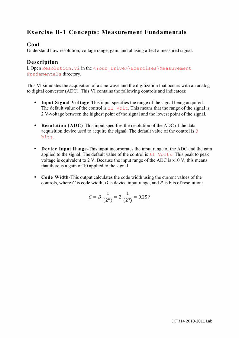
EKT3142010‐2011Lab

Exercise B-1 Concepts: Measurement Fundamentals Goal Understand how resolution, voltage range, gain, and aliasing affect a measured signal. Description l. Open Resolution.vi in the <Your_Drive>\Exercises\Measurement Fundamentals directory. This VI simulates the acquisition of a sine wave and the digitization that occurs with an analog to digital convertor (ADC). This VI contains the following controls and indicators:

• Input Signal Voltage-This input specifies the range of the signal being acquired. The default value of the control is ±1 Volt. This means that the range of the signal is 2 V-voltage between the highest point of the signal and the lowest point of the signal.

• Resolution (ADC)-This input specifies the resolution of the ADC of the data

acquisition device used to acquire the signal. The default value of the control is 3 bits.

• Device Input Range-This input incorporates the input range of the ADC and the gain

applied to the signal. The default value of the control is ±l Volts. This peak to peak voltage is equivalent to 2 V. Because the input range of the ADC is x10 V, this means that there is a gain of 10 applied to the signal.

• Code Width-This output calculates the code width using the current values of the

controls, where C is code width, D is device input range, and R is bits of resolution:

𝐶 = 𝐷.1

(2!) = 2.1(2!) = 0.25𝑉

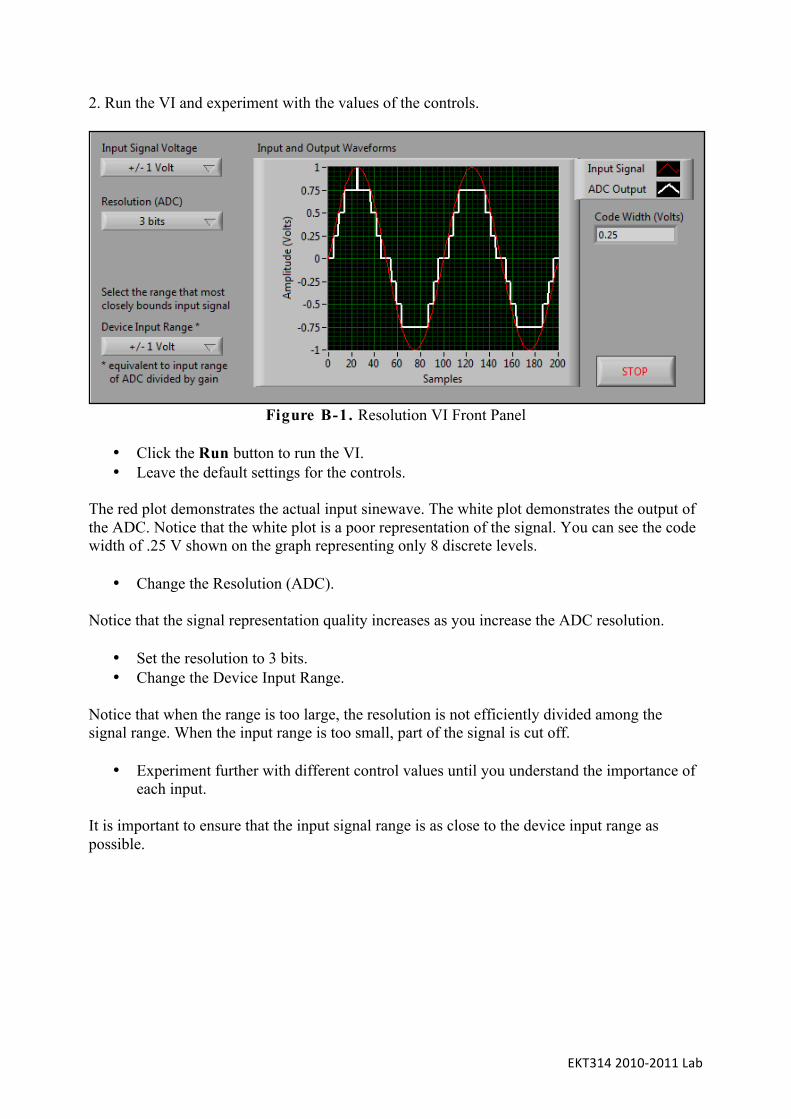
EKT3142010‐2011Lab

2. Run the VI and experiment with the values of the controls.

Figure B-1. Resolution VI Front Panel

• Click the Run button to run the VI. • Leave the default settings for the controls.

The red plot demonstrates the actual input sinewave. The white plot demonstrates the output of the ADC. Notice that the white plot is a poor representation of the signal. You can see the code width of .25 V shown on the graph representing only 8 discrete levels.

• Change the Resolution (ADC). Notice that the signal representation quality increases as you increase the ADC resolution.

• Set the resolution to 3 bits. • Change the Device Input Range.

Notice that when the range is too large, the resolution is not efficiently divided among the signal range. When the input range is too small, part of the signal is cut off.

• Experiment further with different control values until you understand the importance of each input.

It is important to ensure that the input signal range is as close to the device input range as possible.

EKT3142010‐2011Lab

3. Using the Resolution VI, determine the code width of an input signal that varies between ±0.8 V using a DAQ device with a resolution of 16 bits. Assume that gain is efficiently applied. Code Width: 4. Determine the code width of an input signal that varies between ±10 V using a DAQ device with a resolution of 8 bits. The device input range is set to ±10 V. Code Width: 5. lf the device input range is ±l V, and the resolution is 12 bits, what is the largest input signal you can read without cutting off the input signal? Input Signal Range: 6. Stop and close the Vl when you are finished. 7. Open Aliasing.vi in the <Your_Drive>\Exercises\Measurement Fundamentals directory. This VI simulates the acquisition of a waveform at a specific sampling frequency. As you adjust the sampling frequency and the frequency of the acquired waveform, you can observe the Nyquist Theorem in effect. This VI contains the following controls:

• Original Signal o Frequency - This input specifies the frequency of the signal being acquired. You

can increase or decrease this frequency by turning the knob. o Sampled Waveform - The input allows you to choose between a sine wave or a

square wave. Use the sine wave input to experiment with the Nyquist Theorem, and the square wave to understand how the sampling frequency affects shape recovery.

• Sampled Signal

o Sampling Rate (Hz) - This input specifies the rate at which the DAQ device takes a sample of the acquired signal. According to the Nyquist Theorem, this rate should be at least twice the frequency of the sampled signal.

EKT3142010‐2011Lab

8. Run the VI and experiment with the values of the controls until the acquired frequency is wrong.

Figure B-2. Aliasing VI Front Panel

• Set the Waveform Type to Sine . • Set the Sampling Rate Hz to 10 MS/s (megasamples per second). • Adjust the Frequency of the Original Signal, starting at the lowest frequency, and

moving up until the frequency reported on the top chart is no longer correct. Notice how the Sampled plot becomes more distorted as you increase the Frequency of the Original Signal. After you have passed the Nyquist frequency (5 MHz in this case), the frequency recorded is no longer correct. This is an example of aliasing.

9. Try other values for the controls using a sine wave. 10. Set the Waveform Type to Square . Modify the controls to see how shape recovery is affected by the sampling frequency and the frequency of the signal. ll. Stop and close the VI when you are finished. End of Exercise B-1

EKT3142010‐2011Lab

Exercise C-1 Concept: CAN Device Setup

Just read through. We do not have CAN device. Goal Connect CAN hardware and use MAX to view and test a CAN device. Description The exercises in this appendix use a 2-port CAN interface device and a CAN Demo Box. In this exercise, you set up your hardware, observe the configuration of the CAN device in MAX, and run a self-test to verify that the device functions correctly. l. Connect the CAN hardware.

• Connect Port 1 on your CAN interface to the CAN input on the CAN Demo Box using a CAN cable.

• Connect the cable from your DAQ device to the 68-pin terminal on the CAN Demo Box.

• Use a wire to connect the following terminals on the CAN Demo Box. — Gen terminal of the Function Generator — Ch 0 terminal of the Analog In to CAN

2. Explore the CAN device and ports in MAX.

• Launch MAX. • Expand Devices and Interfaces . The PCI-CAN/2 device is your CAN Interface

Device. • Expand PCI-CAN/2 . CAN0 and CANI are physical ports on your CAN device. A

single port interface has only one item.

EKT3142010‐2011Lab

• Select CAN0 and click the Properties button to display the Port Properties dialog box.

Figure C-1. Port Properties Dialog Box Note The Port Properties dialog box allows you to change the baud rate and other

properties of the CAN Interface. The settings are already correct for the current configuration. You also can access the Port Properties dialog box by right-clicking a port and selecting Properties from the shortcut menu.

• Click OK to close the dialog box.

3. Test the CAN Interface Device.

• Select PCI-CAN/2 and observe the value of the Test Status property. The Test Status property displays Untested until you execute a self-test.

• Click the Self-test button located above the list of properties. • Observe the value of the Test Status property after the test completes. Also notice that a

small blue circle with a white check appears above the bottom right corner of the PCI-CAN/2 icon in the Configuration tree, indicating that the device has passed the self-test.

End of Exercise C-1

EKT3142010‐2011Lab

Exercise C-2 Channel Configuration

Just read through. We do not have CAN device. Goal Learn how to load and test channels in MAX. Description Load channels from either an NI CAN database file or a Vector CAN Database tile into MAX. Investigate the properties of messages and channels. Read data on a specific channel using MAX Test Panels. Finally, use the built-in CAN Bus Monitor feature in MAX to monitor the frame data being sent along the CAN bus. 1. Launch MAX and expand Data Neighborhood. 2. Load the database tile for the CAN Demo Box.

• Right-click CAN Channels and select Import from CANdb File .

• Navigate to <Your_Drive>\Exercises\CAN\CAN Demo Box.dbc. Tip You could choose to import the .ndc database files instead. To do so, select Load

Channel Configuration instead of Import from CAN db File .

• Select Add All Messages and Channels .

EKT3142010‐2011Lab

• Click Import. • Click Done .

3. Test a channel in MAX

• Expand CAN Channels . A list of messages with predehned channels appears. Use these channels to communicate with your CAN Demo Box through your CAN Interface.

• Expand the message WAVEFORM0_SAW0_SWITCHES_FROM_CDB (0x710) to see the channels in that message, as shown in Figure C-2.

Figure C-2. WAVEFORM0_SAW0_SWITCHES_FROM_CDB (Ox710) Message

• Select the AnalogInToCANCh0 channel. • Click the Test Panel button.

Tip You also can right-click the channel name and select Test Panel from the shortcut

menu.

• Click the Read tab if it is not already selected.

EKT3142010‐2011Lab

• Click the Start button to begin reading continuously. If the test panel is already reading when you open it, the start button is disabled and you do not need to click it.

Tip A periodic signal should appear. You can see the signal better by changing the scaling to

Auto.

• Experiment with changing the settings on the demo box itself. Use the Menu Select button to scroll through the different options.

o Click the Menu Select button until you see Func Gen Output. o Click the <+> and <-> buttons to change which type of signal the Function

Generator outputs. Select from the following choices-Sine, Square, and Triangle. The screen displays which type is currently being output.

o Click the Menu Select button again until you see Func Gen Freq. o Click the <+> and <-> buttons to increase and decrease the frequency of the

signal the Function Generator outputs. • Click the Stop button in the MAX test panel to finish reading. • Click the Close button to exit the Test Panel.

EKT3142010‐2011Lab

4. Monitor the CAN bus • Expand My System»Devices and Interfaces»PCI-CAN/2 . When selected, the

device’s properties display in the window to the right. • Expand PCI-CAN/2 and select CAN0 . On the right, notice a list of attributes. • Click the Bus Monitor button located above the attributes. • Click the Start button to begin monitoring the CAN bus. If monitoring is already

active, a Stop button appears in place of the Start button and you need not click a button.

Figure C-3. NI-CAN Bus Monitor

• Unplug the connector between the CAN Interface and your demo box. The monitor ceases to show any transmissions because there is nothing being sent to or from the bus.

• Plug in the connector between the CAN Interface and your demo box. Notice periodic transmissions because the demo box is constantly transmitting to and receiving from the CAN Interface.

• Click the Stop button. • Click the Reset button.

5. Save the bus monitor activity to file.

• Click the Options button. • Enable the Stream To Disk checkbox. • Leave the remaining options at their default values. • To specify where to stream the data, click the File Name button in the dialog box and

navigate to a file path. • Click the OK button. • Click the Start button to begin monitoring and logging. • After a few moments, click the Stop button. • Click the Close button to close the bus monitor.

6. Open the log file that you specified in the previous steps and view its contents. End of Exercise C-2

EKT3142010‐2011Lab

Exercise C-3 Read and Write CAN Channels

Just read through. We do not have CAN device. Goal Read and write channels from the CAN device using LabVIEW. Description Complete a VI that reads a single value at a time from the CAN Interface and graphs it on a chart. The channel being read is Analog Input on Channel O of the CAN Demo box. Note Before beginning this exercise, load the CAN Demo Box.ncd or CAN Demo

Box.dbc database into MAX. Also, wire the Function Generator Gen output to the AnalogInToCANCh0 input on the CAN demo box. You completed these steps in a previous exercise.

Implementation Read a Single Channel 1. Open Read CAN Channels VI, located in the <Your_Drive>\Exercises\CAN directory. In the following steps, you complete the block diagram shown in Figure C-4.

Figure C-4. Read CAN Channels VI Block Diagram

EKT3142010‐2011Lab

2. Add the CAN Channel VIs to the block diagram. • Add the CAN Init Start VI to the block diagram to the left of the While Loop. • Right-click the channel list input of the CAN Init Start VI and select

Create»Control . • Right-click the interface input of the CAN Init Start VI and select Create»Control . • Right-click the mode input of the CAN Init Start VI, select Create»Constant. • Select Input from the mode enum constant. • Add the CAN Read VI to the block diagram inside the While Loop. • Select Single Channel»Single Sample»DBL from the pull-down menu on the

CAN Read VI. Tip You also can accomplish this by right-clicking the VI and selecting Select

Type»Single Channel»Single Sample»DBL from the shortcut menu.

• Add the CAN Clear VI to the block diagram to the right of the While Loop. 3. Wire the block diagram as shown in Figure C-4. 4. Switch to the front panel. 5. Test the VI.

• Set the interface control to CAN0 . • Enter AnalogInToCANCh0 into the first array element cf the channel list control.

Tip You also can drag the name of the channel into the array element from MAX. The

channel is found in the message WAVEFORM0_SAW0_FROM_CDB (0x710).

• Run the VI. • Experiment with CAN Demo Box. Change the signal time and frequency. Notice the

changes taking effect on your chart.

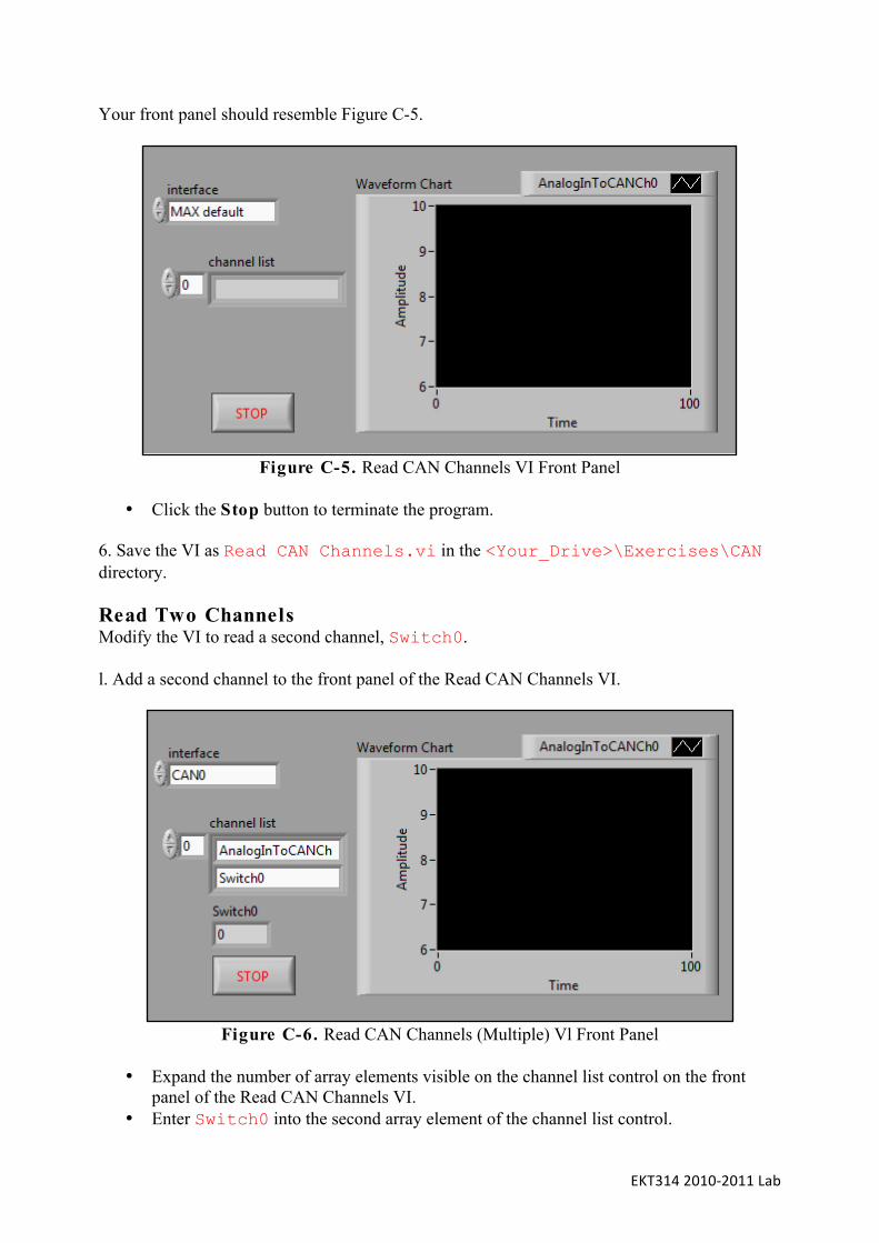
EKT3142010‐2011Lab

Your front panel should resemble Figure C-5.

Figure C-5. Read CAN Channels VI Front Panel

• Click the Stop button to terminate the program.

6. Save the VI as Read CAN Channels.vi in the <Your_Drive>\Exercises\CAN directory. Read Two Channels Modify the VI to read a second channel, Switch0. l. Add a second channel to the front panel of the Read CAN Channels VI.

Figure C-6. Read CAN Channels (Multiple) Vl Front Panel

• Expand the number of array elements visible on the channel list control on the front

panel of the Read CAN Channels VI. • Enter Switch0 into the second array element of the channel list control.

EKT3142010‐2011Lab

• Add a numeric indicator to the front panel and rename it as Switch0. 2. Modify the block diagram as shown in Figure C-7 to display the second channel.

Figure C-7. Read CAN Channels (Multiple) Vi Block Diagram

• Switch to the block diagram. • Delete the wire between the output of the CAN Read VI and the waveform chart. • Select Multiple Channels»Single Sample»lD DBL from the pull-down menu

that appears below the CAN Read VI (the polymorphic VI selector). This specifies that the VI should read an array of doubles, one from each channel, every time that it executes.

• Add an Index Array function to the block diagram. • Using the cursor, drag the border of the Index Array function to expand its size so that it

returns two array elements instead of one. • Wire the multi-chan single-samp 1D dbl output array from the CAN Read VI to

the array input of the Index Array function. • Right-click the index0 input of the Index Array function and select

Create»Constant. • Right-click the index1 input of the Index Array function and select

Create»Constant.

EKT3142010‐2011Lab

• Enter 1 in the second constant. • Connect the first output element of the Index Array function to the waveform chart

indicator terminal and connect the second output element to the Switch0 indicator terminal.

3. Save the VI as Read CAN Channels (Multiple).vi in the <Your_Drive>\Exercises\CAN directory. 4. Switch to the front panel. Test l. Test the VI.

• Run the VI. While it is running, experiment with changing the properties of the function generated by the CAN Demo Box.

• Experiment with changing the state of SwitchO as well. As you toggle the switch (Digital Input O) on the CAN Demo Box, notice that the value of the numeric indicator changes.

2. Use another VI to modify the frequency of the waveform generated by the demo box.

• Open the Write CAN Channels VI, located in the <Your_Drive>\Exercises\CAN directory.

• Ensure that the channel list has one element with the channel name Funcion Generator Frequency.

• Set the interface control to CAN O. • Run the CAN Read Channels VI and the CAN Write Channels VI. • Experiment with changing the Frequency Value control on the CAN Write Channels VI

and see how it affects the chart for the CAN Read Channels VI. 3. Terminate the execution of both VIs by clicking their Stop buttons. End of Exercise C-3

EKT3142010‐2011Lab

Exercise C-4 Synchronize CAN & DAQ

Just read through. We do not have CAN device. Goal Synchronize CAN and DAQ inputs in LabVIEW. Description There are two CAN and DAQ acquisitions inputting data simultaneously. Both the acquisitions are buffered, meaning that the timing is handled on the interface devices. Explore a VI that synchronizes the inputs by routing the clock signal from one of the devices to the other using a Rea1-Time Serial Interface (RTSI) cable to connect the two. 1. Open the Sync CAN & DAQ VI located in the <Exexcises>\LabVIEW Core 1\CAN directory. 2. Switch to the block diagram. 3. Explore the block diagram shown in Figure C-8. Notice that this VI reads from both the CAN and DAQ interfaces and uses RTSI to synchronize the timing.

Figure C-8. Sync CAN & DAO VI Block Diagram

4. Switch to the front panel. 5. Set the control values:

• Interface: CAN0 • Channel List: Anal0gInT0CANCh0

EKT3142010‐2011Lab

• Physical channels: Devl / ai0 • RTSI Terminal: RTSI0 • Sample Rate: 1000 . 00

6. On the CAN Demo Box, attach two wires to jumper between the output of the Functions Generator, the input Analog ln to CAN Ch0, and the input Analog In to DAQ Ch0. 7. Run the Vl. Notice that the signals read from the CAN interface and the DAQ device are perfectly synchronized. To terminate the VI, click the Stop button. 8. Close the VI when you are finished. End of Exercise C-4

EKT3142010‐2011Lab

End of Stage I Exercises