© 2012 Revathi Jambunathan

EFFECT OF HEATING ON SOUND RADIATED FROM A TWO-DIMENSIONAL

MIXING LAYER

BY

REVATHI JAMBUNATHAN

THESIS

Submitted in partial fulfillment of the requirements

for the degree of Master of Science in Aerospace Engineering

in the Graduate College of the

University of Illinois at Urbana-Champaign, 2012

Urbana, Illinois

Advisor:

Professor Daniel J. Bodony

ABSTRACT

High speed mixing layers are known to become quieter when the temperature of the high-speed stream is

increased at constant velocity. In high-speed mixing layers, it is also found that the large-scale instability

waves play an important role in sound radiation. To compute and understand the effect of temperature on

the dynamics of the instability wave, a linear stability analysis is conducted. Using multiple scales expansion

the governing equations are reduced to an eigenvalue problem. However, critical layers arise as a singularity

along the points where the phase velocity of the instability wave becomes equal to the mean flow velocity.

A method of Frobenius analysis showed that the problem has a log singularity which involves a branch

cut. In the region where the instability wave of the mixing layer gets damped, the branch cut crossed

the path of integration. In order to avoid the critical point and its branch cut, the path of integration is

deformed to move around the singularity and away from the branch cut, by mapping the differential equation

onto a complex plane, to compute the eigenvalue. The eigenfunctions, being physical quantities cannot be

computed by integrating along grid point that lie in the complex plane. To address this issue, two approaches

are implemented to compute the eigenfunctions in the damped region. One method involves a power series

approximation using Frobenius method to avoid the critical point and jump across the branch cut. The

second method involves integrating along the real axis until just before the branch cut where the path of

integration is deformed. Linearized Euler calculations are conducted to compute the perturbation quantities

and study the effects of heating on the fluctuations in both the near field and the far-field. It is found that

the amplitude of pressure fluctuation in the far-field decreases with heating. The large entropy fluctuations,

which increase with heating, modify the sound radiation and are believed to play an important role in sound

reduction with increase in temperature of the high-speed stream. Coupling the linear stability theory and

linearized Euler calculations we see that qualitatively the growth rate in the amplitude of the instability

wave agrees with the eigenvalue study from linear stability theory. With heating, the maximum peak of

the amplitude of the instability wave decreases and it also moves upstream, as expected from the upward

movement of the neutral stability point. To compute the far-field solution, a mathematical procedure is

used to compute the directivity of the sound radiation. Directivity is also computed using the analytical

expressions derived from stationary phase method and compared with the pressure perturbations in the

far-field from linearized Euler calculations. It is observed that the sound radiated decreases with increase in

heating and the results from using theory and simulation compare well in the far-field. The sound radiated

from the mixing layer becomes less directional with heating.

ii

To my parents and brother.

iii

ACKNOWLEDGMENTS

At first I would like to thank Professor Bodony for giving me the opportunity to work on this problem and

constantly guiding and steering me in the right direction. The discussions, hints and discovering the whys

and hows would make me come back to my desk with a fresh perspective. Thank you so much Professor

Bodony for teaching me to be systematic in writing and in approaching a scientific problem. I appreciate

your patience and thank you for being an inspiration.

I express my sincere gratitude to Professor Schmitz from the ECE department and Dr. Kato, Director

of the Upward Bound College Prep Academy, for trusting me and giving me an opportunity to work as

a Teaching Assistant to fund my graduate studies. Thank you also to Aaron and Vinay for being great

colleagues to work with in the ECE lab. I would like to thank my group mates, who along the way have

moulded my perceptions of research and approach to problem solving. To Mahesh senior, I cannot thank you

enough for your constructive criticisms and for always being there to discuss and give simple suggestions.

Sincere thank you to Chris for helping me get over some technical hurdles very quickly, the late evening ride

back home, for the very delicious home baked cookies and pies and also for your valuable suggestions on the

thesis draft. Somethings that I have learned from you both will last me for a lifetime! Mahesh junior, thank

you for letting me knock on your door at anytime to ask questions on math and fluid dynamics. Thank you

Qi, for the math discussions as well as the talks on cobras, dragons, elephants and polar bears and crash

course on swimming as an experimental fluid mechanician. The jokes that you and Mahesh share definitely

lightened the atmosphere in the lab. A warm thank you to Ryan for the early morning dose of motivation

and cheer! A word of thanks also to Nishan and Nek for their encouragement.

A heartfelt thank you to my friends Abhishek, Ashish, Ravi for the coffee breaks, discussions on scientific

advancements during world war, sharing the anxieties and celebrating small successes. Pritha, thank you

for being such an understanding and caring roommate and friend. Murthy and Subha, thank you for being

there and I will always cherish the fun filled moments we shared, especially during my first semester. Nithya

akka, Priyanka, Flora, Alwi and Jiju, a big thank you for your constant support from across the globe.

To my small family at Urbana - Shruti didi, Hardik Bhai, Mohit and Sarah, finally the last member will

also graduate. The warmth at home, good food, dinner-together times, chai times and so much fun. I almost

did not miss my real family when I landed here for the first time. Thank you!

Now to my family back at home. Ma, Daddy and Rahul, I constantly feel your presence and love and

it has kept me going always. Without you and your enthusiastic approach towards ups and downs, I could

not have made it anywhere. Sincere thanks to all my friends and family members for their everlasting

encouragement. Last, but not the least, I thank God for everything!

iv

TABLE OF CONTENTS

LIST OF FIGURES . . . . . . . . . . . . . . . . . . . . . . . . . . . . . . . . . . . . . . . . . . . . . . vi

CHAPTER 1 INTRODUCTION . . . . . . . . . . . . . . . . . . . . . . . . . . . . . . . . . . . . . . 11.1 Motivation . . . . . . . . . . . . . . . . . . . . . . . . . . . . . . . . . . . . . . . . . . . . . . 11.2 Historical Perspective . . . . . . . . . . . . . . . . . . . . . . . . . . . . . . . . . . . . . . . . 21.3 Overview of Contribution . . . . . . . . . . . . . . . . . . . . . . . . . . . . . . . . . . . . . . 41.4 Organization of Thesis . . . . . . . . . . . . . . . . . . . . . . . . . . . . . . . . . . . . . . . . 4

CHAPTER 2 LINEAR STABILITY ANALYSIS . . . . . . . . . . . . . . . . . . . . . . . . . . . . . 62.1 Mean Flow and Governing Equation . . . . . . . . . . . . . . . . . . . . . . . . . . . . . . . . 72.2 Multiscale Linear Theory . . . . . . . . . . . . . . . . . . . . . . . . . . . . . . . . . . . . . . 102.3 The Eigenvalue Problem . . . . . . . . . . . . . . . . . . . . . . . . . . . . . . . . . . . . . . . 122.4 Critical Layer . . . . . . . . . . . . . . . . . . . . . . . . . . . . . . . . . . . . . . . . . . . . . 132.5 Instability Wave Solution . . . . . . . . . . . . . . . . . . . . . . . . . . . . . . . . . . . . . . 162.6 Acoustic Far-Field Solution and Directivity . . . . . . . . . . . . . . . . . . . . . . . . . . . . 18

CHAPTER 3 NUMERICAL METHOD . . . . . . . . . . . . . . . . . . . . . . . . . . . . . . . . . . 233.1 Linear Stability . . . . . . . . . . . . . . . . . . . . . . . . . . . . . . . . . . . . . . . . . . . . 233.2 Linearized Euler Calculations . . . . . . . . . . . . . . . . . . . . . . . . . . . . . . . . . . . . 26

CHAPTER 4 RESULTS AND DISCUSSION . . . . . . . . . . . . . . . . . . . . . . . . . . . . . . . 294.1 Linear Stability Results . . . . . . . . . . . . . . . . . . . . . . . . . . . . . . . . . . . . . . . 294.2 Linearized Euler Calculations . . . . . . . . . . . . . . . . . . . . . . . . . . . . . . . . . . . . 344.3 Combining Linearized Euler Simulations and Linear Stability Theory . . . . . . . . . . . . . . 49

CHAPTER 5 CONCLUSION . . . . . . . . . . . . . . . . . . . . . . . . . . . . . . . . . . . . . . . . 575.1 Future Work . . . . . . . . . . . . . . . . . . . . . . . . . . . . . . . . . . . . . . . . . . . . . 58

CHAPTER 6 REFERENCES . . . . . . . . . . . . . . . . . . . . . . . . . . . . . . . . . . . . . . . . 59

v

LIST OF FIGURES

2.1 Instability wave and its associated acoustic radiation . . . . . . . . . . . . . . . . . . . . . . . 72.2 Schematic of mean flow . . . . . . . . . . . . . . . . . . . . . . . . . . . . . . . . . . . . . . . 8

3.1 Path of integration along the real y-axis since the branch cut, .e. the vertical hatch line,extends from the critical point to −∞ parallel to the imaginary y-axis. . . . . . . . . . . . . . 25

3.2 Path of integration, in the complex y-plane, for the stable region of the mixing layer. Thebranch cut, i.e the vertical hatched line, crosses the real y-axis. Therefore, the path ofintegration take a detour to avoid the critical point and the branch cut. . . . . . . . . . . . . 25

4.1 Comparison of variation of the imaginary part of the eigenvalue (growth rate) of the insta-bility wave along the axial direction for different temperature ratios. ( ), Cold mixinglayer (case 1); ( ), isothermal mixing layer (case 2); ( ), hot mixing layer (case 3) ;( ), hot mixing layer (case 4); ( ), hot mixing layer (case 5); and ( ), hot mixinglayer (case 6). . . . . . . . . . . . . . . . . . . . . . . . . . . . . . . . . . . . . . . . . . . . . . 30

4.2 A zoomed in view of the imaginary part of the eigenvalue to observe the neutral stabilitypoint for different temperature ratios. The dotted line is the x-axis that passes throughthe neutral stability points. ( ), Cold mixing layer (case 1); ( ), isothermal mixinglayer (case 2); ( ), hot mixing layer (case 3) ; ( ), hot mixing layer (case 4); ( ),hot mixing layer (case 5); and ( ), hot mixing layer (case 6). . . . . . . . . . . . . . . . . . 31

4.3 Comparison of variation of the real part of the eigenvalue (spatial frequency) of the insta-bility wave along the axial direction for different temperature ratios. ( ), Cold mixinglayer (case 1); ( ), isothermal mixing layer (case 2); ( ), hot mixing layer (case 3) ;( ), hot mixing layer (case 4); ( ), hot mixing layer (case 5); and ( ), hot mixinglayer (case 6). . . . . . . . . . . . . . . . . . . . . . . . . . . . . . . . . . . . . . . . . . . . . 31

4.4 Comparison of variation of the phase speed, cph = Re{ω/α}, of the instability wave alongthe axial direction for different temperature ratios. ( ), Cold mixing layer (case 1);( ), isothermal mixing layer (case 2); ( ), hot mixing layer (case 3) ; ( ), hotmixing layer (case 4); ( ), hot mixing layer (case 5); and ( ), hot mixing layer (case 6). 32

4.5 Propagation of the critical layer as the instability wave advances from the unstable regionto the damped stable region for mixing layers with different temperature ratios. ( ),Cold mixing layer (case 1); ( ), isothermal mixing layer (case 2); ( ), hot mixinglayer (case 3) ; ( ), hot mixing layer (case 4); ( ), hot mixing layer (case 5); and( ), hot mixing layer (case 6). . . . . . . . . . . . . . . . . . . . . . . . . . . . . . . . . . . 33

4.6 A zoomed-in view of the critical layer path near the origin for the mixing layers of differenttemperature ratios. ( ), Cold mixing layer with static temperature ratio = 0.75; ( ),Cold mixing layer (case 1); ( ), isothermal mixing layer (case 2); ( ), hot mixinglayer (case 3) ; ( ), hot mixing layer (case 4); ( ), hot mixing layer (case 5); and( ), hot mixing layer (case 6). . . . . . . . . . . . . . . . . . . . . . . . . . . . . . . . . . 34

vi

4.7 Comparison of the imaginary part of the critical layer near the neutral stability (NS)region with unstable region to the left of the NS point and stable region to the rightof the NS stability point. The dashed real y-axis, ( ), passes through the NS pointsfor each critical layer curve. ( ), Cold mixing layer (case 1) with NS at x = 174;( ),isothermal mixing layer (case 2)with NS at x = 172; ( ), hot mixing layer (case3) with with NS at x = 171; ( ), hot mixing layer (case 4) with NS at x = 168; ( ),hot mixing layer (case 5) with NS at x = 166; and ( ), hot mixing layer (case 6) withNS at x = 164; . . . . . . . . . . . . . . . . . . . . . . . . . . . . . . . . . . . . . . . . . . . . 35

4.8 Comparison of the real part of the derivative of the eigenfunction (pressure disturbance),Re{dζ/dy}, in the unstable region, at x = 150 for the isothermal mixing layer, computedusing two different numerical approaches. ( ), Using Frobenius method to approximatethe solution near near the critical point; ( ), using deformed complex path of integrationto avoid singularity which cuts across the real integration path. . . . . . . . . . . . . . . . . 36

4.9 Comparison of the real part of the derivative of the eigenfunction (pressure disturbance),Re{dζ/dy}, in the stable region, at x = 450 for the isothermal mixing layer, computedusing two different numerical approaches. The function is discontinuous at the point wherethe branch cut crosses the real y-axis and it is seen from the slope of the function ζ inthe above figure. ( ), Using Frobenius method to approximate the solution near nearthe critical point; ( ), using deformed complex path of integration to avoid singularitywhich cuts across the real integration path. . . . . . . . . . . . . . . . . . . . . . . . . . . . . 37

4.10 Comparison of the eigenfunction (pressure disturbance), |ζ|, at y = 0 for the isothermalmixing layer computed using two different numerical approaches. ( ), Using Frobeniusmethod to approximate the solution near near the critical point; ( ), using deformedcomplex path of integration to avoid singularity which cuts across the real integration path. 38

4.11 Comparison of the eigenfunction (pressure disturbance), ζ, in the stable region, at x =450 for the isothermal mixing layer, computed using two different numerical approaches.( ), Using Frobenius method to approximate the solution near near the critical point;( ), using deformed complex path of integration to avoid singularity which cuts acrossthe real integration path. . . . . . . . . . . . . . . . . . . . . . . . . . . . . . . . . . . . . . . 39

4.12 Comparison of the eigenfunction (pressure disturbance), |ζ|, at y = 0 for the mixing layerswith different temperature ratios. The region to the right of the vertical dashed line ( ),is the sponge region where queiscient boundary condition is implemented in the linearizedEuler Calculations. ( ), Cold mixing layer (case 1); ( ), isothermal mixing layer(case 2); ( ), hot mixing layer (case 3) ; ( ), hot mixing layer (case 4); ( ), hotmixing layer (case 5); and ( ), hot mixing layer (case 6). . . . . . . . . . . . . . . . . . . 40

4.13 Instantaneous pressure perturbation for cold mixing layer with static temperature ratio= 0.75 showing the radiation of pressure fluctuations away from mixing layer. The warmcolors (red) represent high values of pressure fluctuation amplitude, with a maximum valueof p′ = 1.5× 10−3. . . . . . . . . . . . . . . . . . . . . . . . . . . . . . . . . . . . . . . . . . . 41

4.14 Instantaneous pressure perturbation for isothermal mixing layer with static temperatureratio = 1.00 showing the radiation of pressure fluctuations.The warm colors (red) representhigh values of pressure fluctuation amplitude, with a maximum value of p′ = 1.5× 10−3. . . . 41

4.15 Instantaneous pressure perturbation for hot mixing layer with static temperature ratio= 1.25 showing the radiation of pressure fluctuations.The warm colors (red) represent highvalues of pressure fluctuation amplitude, with a maximum value of p′ = 1.5× 10−3. . . . . . . 42

4.16 Instantaneous pressure perturbation for hot mixing layer with static temperature ratio= 1.75 showing the radiation of pressure fluctuations.The warm colors (red) represent highvalues of pressure fluctuation amplitude, with a maximum value of p′ = 1.5× 10−3. . . . . . . 42

4.17 Instantaneous pressure perturbation for hot mixing layer with static temperature ratio= 2.25 showing the radiation of pressure fluctuations.The warm colors (red) represent highvalues of pressure fluctuation amplitude, with a maximum value of p′ = 1.5× 10−3. . . . . . . 43

vii

4.18 Instantaneous pressure perturbation for hot mixing layer with static temperature ratio= 2.75 showing the radiation of pressure fluctuations.The warm colors (red) represent highvalues of pressure fluctuation amplitude, with a maximum value of p′ = 1.5× 10−3. . . . . . . 43

4.19 Comparison of the scaled root-mean-square pressure perturbation from the linearized Eulercalculations at y = 0 for mixing layers with different temperature ratios. The values areplotted till x = 725, beyond which the sponge boundary (quiescient) condition is imposed.( ), cold mixing layer (case 1) with peak amplitude at x = 219; ( ), isothermalmixing layer (case 2) with peak amplitude at x = 216; ( ), hot mixing layer (case 3)with peak amplitude at x = 207; ( ), hot mixing layer (case 4) with peak amplitude atx = 187; ( ), hot mixing layer (case 5) with peak amplitude at x = 177; and ( ),hot mixing layer (case 6) with peak amplitude at x = 171. . . . . . . . . . . . . . . . . . . . 44

4.20 Comparison of the scaled root-mean-square streamwise velocity perturbation from the lin-earized Euler calculations, at y = 0, for mixing layers with different temperature ratios.The values are plotted till x = 725, beyond which the sponge boundary (quiescient) condi-tion is imposed. ( ), Cold mixing layer (case 1); ( ), isothermal mixing layer (case2); ( ), hot mixing layer (case 3) ; ( ), hot mixing layer (case 4); ( ), hot mixinglayer (case 5); and ( ), hot mixing layer (case 6). . . . . . . . . . . . . . . . . . . . . . . . 45

4.21 A zoomed-in view of root-mean-square streamwise velocity perturbation near its peakamplitude scaled such that its peak value is equal to unity to put all the cases beingstudied on an equal footing. ( ), Cold mixing layer (case 1) with peak at x = 276;( ), isothermal mixing layer (case 2) with peak at x = 271; ( ), hot mixing layer(case 3) with peak at x = 260; ( ), hot mixing layer (case 4) with peak at x = 242;( ), hot mixing layer (case 5) with peak at x = 233; and ( ), hot mixing layer (case6) with peak at x = 228. . . . . . . . . . . . . . . . . . . . . . . . . . . . . . . . . . . . . . . 46

4.22 Comparison of the scaled root-mean-square vertical velocity perturbations from the lin-earized Euler calculations, at y = 0, for mixing layers with different temperature ratios.The values are plotted till x = 725, beyond which the sponge boundary (quiescient) condi-tion is imposed. ( ), Cold mixing layer (case 1); ( ), isothermal mixing layer (case2); ( ), hot mixing layer (case 3) ; ( ), hot mixing layer (case 4); ( ), hot mixinglayer (case 5); and ( ), hot mixing layer (case 6). . . . . . . . . . . . . . . . . . . . . . . . 47

4.23 Comparison of the scaled root-mean-square entropy perturbations from the linearized Eulercalculations, at y = 0, for mixing layers with different temperature ratios. The values areplotted till x = 725, beyond which the sponge boundary (quiescient) condition is imposed.( ), Cold mixing layer (case 1); ( ), isothermal mixing layer (case 2); ( ), hotmixing layer (case 3) ; ( ), hot mixing layer (case 4); ( ), hot mixing layer (case 5);and ( ), hot mixing layer (case 6). . . . . . . . . . . . . . . . . . . . . . . . . . . . . . . . 47

4.24 Comparison of the scaled root-mean-square density perturbations from the linearized Eulercalculations, at y = 0, for mixing layers with different temperature ratios. The values areplotted till x = 725, beyond which the sponge boundary (quiescient) condition is imposed.( ), Cold mixing layer (case 1); ( ), isothermal mixing layer (case 2); ( ), hotmixing layer (case 3) ; ( ), hot mixing layer (case 4); ( ), hot mixing layer (case 5);and ( ), hot mixing layer (case 6). . . . . . . . . . . . . . . . . . . . . . . . . . . . . . . . 48

4.25 Comparison of |Aoeiθ| at y = 0 for mixing layers with different temperature ratios. Thevalues are plotted till x = 725, beyond which the sponge boundary (quiescient) conditionis imposed. ( ), Cold mixing layer (case 1); ( ), isothermal mixing layer (case 2);( ), hot mixing layer (case 3) ; ( ), hot mixing layer (case 4); ( ), hot mixinglayer (case 5); and ( ), hot mixing layer (case 6). . . . . . . . . . . . . . . . . . . . . . . . 50

4.26 Comparison of the amplitude of the instability wave in a log scale, log10|Ao|, at y = 0, formixing layer with different temperature ratios. ( ), Cold mixing layer (case 1); ( ),isothermal mixing layer (case 2); ( ), hot mixing layer (case 3) ; ( ), hot mixinglayer (case 4); ( ), hot mixing layer (case 5); and ( ), hot mixing layer (case 6). . . . . 51

viii

4.27 Amplitude (Ao) of the instability wave at y = 0 for the cold mixing layer (case 1) withstatic temperature ratio = 0.75. The location of peak amplitude at x = 219 . . . . . . . . . . 52

4.28 Amplitude (Ao) of the instability wave at y = 0 for the isothermal mixing layer (case 2)with static temperature ratio = 1.00. The location of peak amplitude at x = 216 . . . . . . . 52

4.29 Amplitude (Ao) of the instability wave at y = 0 for the hot mixing layer (case 3) withstatic temperature ratio = 1.25. The location of peak amplitude at x = 207 . . . . . . . . . . 53

4.30 Amplitude (Ao) of the instability wave at y = 0 for the hot mixing layer (case 4) withstatic temperature ratio = 1.75. The location of peak amplitude at x = 187 . . . . . . . . . . 53

4.31 Amplitude (Ao) of the instability wave at y = 0 for the hot mixing layer (case 5) withstatic temperature ratio = 2.25. The location of peak amplitude at x = 177 . . . . . . . . . . 54

4.32 Amplitude (Ao) of the instability wave at y = 0 for the hot mixing layer (case 6) withstatic temperature ratio = 2.75. The location of peak amplitude at x = 171 . . . . . . . . . . 54

4.33 Comparison of directivity, (D(θ)), in the acoustic field for the mixing layer with differenttemperature ratios. ( ), Cold mixing layer (case 1) with maxD(θ) = 5 × 10−9 atθ = 15.5; ( ), isothermal mixing layer (case 2) with maxD(θ) = 2.63×10−9 at θ = 15.28;( ), hot mixing layer (case 3) with maxD(θ) = 1.59 × 10−9 at θ = 15.23; ( ), hotmixing layer (case 4) with maxD(θ) = 6.296×10−10 at θ = 15.14; ( ), hot mixing layer(case 5) with maxD(θ) = 3.312× 10−10 at θ = 15.63; and ( ), hot mixing layer (case6) with maxD(θ) = 5.765× 10−10. . . . . . . . . . . . . . . . . . . . . . . . . . . . . . . . . . 55

4.34 Directivity, (D(θ)), in the acoustic field for the hot mixing layer (case 6). The radiationpeaks at θ = 96.37°where max(D(θ)) = 2.8×10−10. The first peak occurs at θ = 16.22°withD(θ) = 2.181× 10−10. . . . . . . . . . . . . . . . . . . . . . . . . . . . . . . . . . . . . . . . . 56

ix

CHAPTER 1

INTRODUCTION

1.1 Motivation

The globalization of business and the emergence of new markets around the world have prompted aerospace

companies to focus more on fast and efficient business transportation. At present, it is estimated that over

30 million commercial flights carrying 1.8 billion passengers are flown every year throughout the world. The

sprawl of communities and increased air travel demands has led to larger airports, which are built in close

proximity to residential properties. The aerodynamic noise of airplanes during take-off and landing continues

to be a critical factor in the design, development and certification of aircraft, especially supersonic transport

aircraft.

The success of the supersonic jets depends on its ability to be safe, technically feasible, environmentally

friendly and economically viable. Increased noise in supersonic aircraft is a serious challenge and the engine

must meet or exceed the noise and emissions requirements. The Federal Aviation Administration (FAA)

continues to impose stringent margins for landing and take-off noise and NOx and CO2 emissions that are the

current challenges faced during the design and development of future aircraft. Entities like Boeing, Northrop

Grumman, NASA, and Gulfstream have dedicated research to aid in the development of environmentally

friendly supersonic aircraft.

The excessive noise from jet engines was initially seen as merely a nuisance and its impact on the

environment was ignored by certifying agencies and governments. Research emerging in the 1970’s linked

noise pollution to negative ecological impacts as well as serious health effects in humans [1]. Adverse effects

in humans include hearing loss, tinnitus and hypertension. Noise pollution has been linked to the disruption

of the feeding and nesting habits of wildlife (mostly birds) near airports.

There are various sources of noise present in an aircraft [2]. The major sources are: the airframe, the

main fan in the engine, turbomachinery and the jet-engine exhaust. During take-off, jet noise continues to be

a dominant source of sound and therefore jet noise reduction is an important research topic, and motivation

of the current study.

Jet noise prediction is a first step for such an effort. However, both theoretical and numerical approaches

suffer from the difficulties caused by jet turbulence as the source of sound. To avoid the complexities of the

study, it is necessary to make some simplifications. As a first step towards simplification, we will study noise

generation in a two-dimensional mixing layer.

The mixing layer that forms between two streams flowing with different velocities is an important canon-

ical flow that is ideal to study the dynamics of inhomogenous turbulence. Since the process of sound

generation and turbulent mixing are connected, the study of mixing layers has significant implications for

1

applications such as the noise radiation from near-nozzle region of high speed turbulent jets.

The phenomenon of sound generation by spatially growing instability waves in high-speed flows has been

investigated by Tam [3] and [4] and [5]. In the present study, we study the effect of heating on sound radiated

by instability waves, in a non-parallel, non-isothermal, two-dimensional mixing layer.

1.2 Historical Perspective

As the attempt to improve the efficiency of jet engines and speed of the aircraft began, research concurrently

aimed at countering its adverse side effects, namely the mitigation of the noise produced by the turbulent

exit flow. Beginning in the 1950’s, Lighthill [6] initiated the study of unsteady fluid motion to understand

the process of aerodynamic sound generation, which is the core research topic in aeroacoustics. This theory

allowed for prediction of sound, but only when the source term, (quadrupole-like) is known a priori.

High speed turbulent shear layers are ideal for studying turbulence and its associated noise generating

mechanisms. Low-speed mixing layers have been studied extensively and is summarized in the review of Ho

and Huerre [7]. The initial growth of the mixing layer is very sensitive to the state of the boundary layer

and whether any external forcing or acoustic reflection is present [8]. The width of the mixing layer grows

asymptotically from where the two streams meet in the absence of an externally imposed pressure gradient.

In the past, a number of investigators e.g Tam [9, 10], Bishop, Ffowcs Williams and Smith [11], and Morris

[12] have suggested, on theoretical grounds, that flow instabilities could be the dominant noise-generation

mechanism in supersonic jets. This idea was confirmed by McLaughlin, Morrison and Troutt [13, 14] in

low-Reynolds number supersonic jet experiments. More recently, the same was confirmed for experiments at

moderately high Reynolds number, by Troutt and McLaughlin [15]. It has also been known that in turbulent

shear flows, large-scale coherent structures exist. The growth of the large scale structures and that of the

time-averaged mixing layer, was a function of the density ratio ρ2/ρ1 across the mixing layer [16]. They

concluded that the compressibility effects were effective in altering the mixing growth rate and, subsequently,

a large number of investigations were conducted to better understand this. These studies suggested that the

mixing layer growth rate, dδ/dx, was a function of the convective Mach number,Mc, which was loosely linked

to he convection velocity of the large-scale structures of the mixing layer. Various definitions for Mc exist;

one of the most commonly used is that of Papamoschou and Roshko [17] and is Mc = (U1 − U2)/(a1 + a2),

where a1 and a2, are the speeds of sound either side of the mixing layer.

By focusing on the parameter Mc, the separate effects of velocity ratio and density ratio across high-

speed compressible mixing layers have not been examined in great detail, except for the effect of the latter

on mixing layer growth. Experimentally it is challenging to measure thermodynamic fields without intrusive

diagnostics at the same level of spatiotemporal resolution as provided by partical image velocimetry. Recent

enhancements to the measurement capabilities are changing this, however. In low-speed flows, wire-based

techniques are available for simultaneous temperature-velocity measurement.

There is direct evidence that the dynamic behavior of large-scale structures can be modeled analytically

by linear stability theory [18]. However, classical hydrodynamic stability theory of a compressible flow does

not predict acoustic radiation by instability waves. [19, 20, 21, 22]. This issue was addressed by Tam and

Morris in [3]. The point of departure of their anaylsis lies in their recognition that to determine sound

radiation, a global solution of the entire wave propagation phenomenon is necessary. A global solution is

2

obtained by implementing matched asymptotic expansion and taking a Fourier transform which is uniformly

valid in all directions in the far-field. The explanation of the noise generation mechanism related to the

instability wave is given in chapter 2.

The method of multiple-scales expansion has proven to be useful for the computation of instability waves

at low-to-moderate speed flows. However for high subsonic and supersonic flows this method breaks down.

specifically, when an instability wave, having supersonic phase velocity relative to the ambient speed of

sound, becomes neutrally stable as it propagates downstream, this method cannot be used to continue into

the damped region. This problem has been described as the ’damped supersonic wave’ phenomenon in [4].

It occurs when the phase velocity of the instability wave remains supersonic even when the wave enters the

damped region. At this point, it is observed that a local singularity, called critical layer arises when the phase

velocity of the instability wave becomes equal to the mean velocity. A review on the developments in critical

layer is given in [23]. In the damped region, the branch cut associated with the problem crosses the path

of integration. This problem has been addressed by [4, 5, 24, 25] and [26]. Prof.Tam [4] and Prof.Schmid

[26] deform the integration contour near the critical layer so as to avoid the singularity to obtain the linear

stability solution. On the other hand, Boyd [24], Gill [25] solve the eigenvalue value problem involved in the

instability wave solution in two steps; first to find the eigenvalue, the domain of integration is mapped into

the complex plane and in a second step, depending on the location of the singularity, called critical layer, the

eigenfunction is determined. If the critical layer is on the real-axis, a gaussian complex detour that moves

around the critical point can be implemented. However, if the critical point is in the complex plane, a local

power series approximation along with finite difference method can be used to compute the instability wave

solution accounting for the discontinuity in solution across the critical layer. Recently, [27] has worked on

using the finite difference method coupled with Frobenius power series approximation to solve the shear layer

problem in an axisymmetric, diverging jet. In this work, the contribution of the critical layer in the sound

generation process has also been considered.

Very little is known about the instantaneous or two-point space time correlations of velocity with the

thermodynamic field in any high-speed turbulent flow, except for a few computational efforts [28, 29] and

[30] and recent causality experiments related to jet noise [31, 32]. The successful modeling of noise sources

in compressible turbulent flows depends crucially on the space-time correlations of the fluctuations involved

and it was recently identified that the velocity-temperature correlation is the largest contributor to noise

prediction uncertainty [33]. It is a commonly held assumption that the <u′T ′> space-time correlation is the

same as <u′u′>, within a proportionality constant, but there is not simulation or experimental justification

for this [34]. As a result, current noise prediction methodologies, aside from direct numerical or large-eddy

simulation, are unable to predict the trends in jet noise with heating without calibration.

The density ratio of the two streams being mixed plays a significant role in the dynamics of the mixing

layer. Variable density mixing layers arise in the context of heated jets where the temperature ratio is an

important parameter and has been identified to affect noise radiation characteristics. It has been observed

that jet noise radiation increases with increase in the temperature ratio in subsonic jets. On the contrary,

in the high subsonic and supersonic jets, an opposite trend is observed in the large-eddy simulation results

in [29], that shows a decrease in radiation noise with increase in temperature ratio. However, the cause for

the reduction in noise radiation is still to be understood.

In the present work, we consider the main principles of Tam’s instability wave theory and extend the

theoretical analysis in [3] to account for the temperature effects of a heated mixing layer. To solve for the

3

instability wave solution, first the eigenvalue is determined using the method suggested by Boyd in [24]

where the equations are mapped into the complex domain to move around singular points that occur in

the stable region. With the eigenvalue known, two different approaches were implemented to determine the

solution to an ordinary differential equation that governs the eigenvalue problem. One method involved

implementation of contour deformation in the complex plane just before the critical layer and the second

involved a combination of the finite difference method and a local power series expansion to compute the

solution in the damped region for the supersonic mixing layer. The solution is further extended into the

far-field to compute the acoustic radiation.

1.3 Overview of Contribution

There are four primary objectives in the present work. The first is to implement a mathematical procedure,

developed by [3], capable of calculating the global solution to the excited instability waves and their far-field

effects. This procedure is further extended to non-isothermal mean flow to capture the temperature effects

on the acoustic radiation. The second is to examine carefully the dynamic role played by the entropy field

through the numerical simulation and a multi-scale linear theory. Here the mean flow is modified to model

the cold, isothermal and heated jets and the effects of initial disturbances are studied by running linearized

Euler calculations on the spatially developing mean flow. The third is to verify that the Euler calculations

can be used in conjunction with the linear theory to study the acoustic behaviour of mixing layers, which

will in future be extended to study jet noise. The fourth objective is to verify the suggestion that large

coherent disturbances are efficient noise radiators by comparing results from linear theory and simulations.

1.4 Organization of Thesis

The thesis is organized as follows

Chapter 2 introduces the physical aspects of the problem and develops the mathematical procedure used

in determining the instability wave solution and its associated sound field. The mean flow and the governing

equations used in the present study are discussed in section 2.1. The multiscale linear theory in section 2.2

reduces the governing equation in section 2.1 to an eigenvalue problem, (solved in section 2.3) formed by

the zeroth-order terms from the multiple-scale expansion and their boundary condition. The critical layer

that arises in the shear layer is discussed in 2.4 and a mathematical analysis to understand the nature of

the singularity is provided in section 2.4.1. Section 2.5 uses the first order terms from the multiple-scale

expansion to determine the amplitude of the instability wave and the solution of the pressure perturbation

up to order unity. An extension of the instability wave solution to give a uniformly valid solution in the

far-field is presented in section 2.6.

In chapter 3, the numerical method involved in the implementation of the theory is presented. The

solution procedure to obtain the eigenvalue and eigenfunction in the stable region of the mixing layer to

compute the amplitude of the instability wave is presented in section 3.1. The fluid solver that computes the

perturbation quantities by solving the linearized Euler equations is discussed in section 3.2. The methodology

used in computing the directivity and instability wave amplitude function by combining the results from the

4

linearized Euler simulations and the stability theory is presented in sections 3.2.3 and 3.2.4.

The results of the study is presented in chapter 4. The method outlined in chapter 3 is implemented and

combined with the results from the linearized Euler calculations. The effect of heating on the eigenvalue,

the growth and decay of the instability wave and the propagation of the critical layer within the shear zone

from the unstabe to stabe region is discussed in section 4.1. The perturbations quantities and change in

their dynamics with heating is analysed in section 4.2. The solutions from theory and simulation are coupled

in section 4.3 and the role played by entropy fluctuations on the large-scale dynamics and sound field is

discussed.

Finally chapter 5 gives an overview of the major results of the present study and provides a larger scope

for the current work.

5

CHAPTER 2

LINEAR STABILITY ANALYSIS

In free shear flows, such as mixing layers or jets, the mean flow diverges slowly in the flow direction, owing to

the entrainment of ambient fluid. Over the initial region, when the shear layer is thin and the mean-velocity

gradient is large, the amplitude of an excited instability wave grows very rapidly. As the wave propagates

downstream, the growth-rate decreases. This is because, as the flow slowly diverges, the transverse ve-

locity gradient is gradually reduced. Eventually at some point downstream, the growth rate of the wave

becomes zero. On propagating further downstream, the wave becomes damped. Its amplitude decreases

as it continues to propagate until it becomes vanishingly small. The growth and decay of the wave ampli-

tude is extremely important to the sound radiating process. For a fixed-frequency instability wave, whose

amplitude undergoes growth and decay spatially, its wavenumber spectrum is broadband and not discrete.

For high subsonic and supersonic mean flow, some of these wavenumbers will be moving with supersonic

phase velocities. These supersonic phase disturbances, by the wavy-wall analogy, lead to acoustic radiation.

However, the method of multiple-scales instability wave solution does not predict sound radiation. This is

mainly because the boundary conditions in the multiple-scales problem are such that the wave disturbances

decay to zero in the far-field region. Application of this boundary condition cannot yield the acoustic field

associated with the instability wave. Moreover, the acoustic disturbances propagate in all directions and so

all spatial coordinates must be treated on an equal footing. The method of multiple-scales which scales the

coordinates differently, is therefore not appropriate to compute acoustic radiation from instability waves.

Tam and Morris [3] therefore proposed to construct an extended solution of the multiple-scales, instability

wave solution by the method of Fourier transform. This extended solution is uniformly valid in all direction

far away from the mixing layer. They were able to calculate the acoustic radiation associated with the

excited instability waves in compressible two-dimensional isothermal mixing layers.

The non-linear effects are neglected in the present analysis. As given in [4], the nonlinear effects may be

divided into non-linear interaction of the instability waves and the mean-flow and the self-interaction of the

instability waves. The former modifies the mean-flow which further modifies the characteristic of the insta-

bility wave. To account for this interaction, the mean-flow based on empirical data is used in the analysis.

The effects of non-linear self-interaction are neglected as a first approximation. The spatial growth, peaking

and decay of the amplitude of an instability wave in the flow direction of the mixing layer, are controlled by

the local linear properties of the wave, which are determined by the local mean-flow profile.

The analysis here is extended to non-isothermal, two-dimensional, spatially growing supersonic as well as

subsonic mixing layers. The following steps are followed in the analysis: (i) the instability-wave solution is

developed using multiple-scale method and (ii) an analytical continuation of the solution in the far-field is

6

X

InstabilityWave

SoundRadiation

Figure 2.1: Instability wave and its associated acoustic radiation

constructed by taking a Fourier transform to obtain a global acoustic solution which is uniformly valid in

the outer region.

2.1 Mean Flow and Governing Equation

The spatial evolution of a small-amplitude instability wave in a pre-existing two-dimensional supersonic

diverging mixing layer is considered. We follow the approach of [3] to obtain the instability wave solution

and its associated sound field. The mean flow profile is sketched in figure 2.2. This mixing layer is formed

between the stationary medium in the upper half-plane and a uniform-flow with non-zero Mach number in

the lower half-plane. The static pressure is assumed to be constant throughout the flow. The mean flow in

the lower-half plane follows from the observation that most high Reynolds number mixing layers are turbu-

lent with a growth rate dδ/dx that is a function of the convective Mach number, Mc = U2/(a1 + a2), which

is related to the acoustic Mach number, Ma = U2/a1, and the static temperature ratio, T2/T1. We thus

propose the following mean flow based on empirical data :

U(x, y) =Ma

2

(

1− erf

{

y

δ(x)

})

(2.1a)

V (x, y) = (2.1b)

P (x, y) =1

γ − 1(2.1c)

ρ(x, y) =γP∞

(γ − 1)T (x, y)(2.1d)

7

X

ym

yn

Figure 2.2: Schematic of mean flow

where,

δ(x) =

{

1/√π, x ≤ xa

1/√π + 2S(1− erf (0.6Mc))x, x ≥ xc

where S = 0.10 is an estimate of incompressible turbulence mixing layer growth [35] and 1 − erf (0.6Mc) is

the compressibility correction to it. The mixing layer is parallel for x ≤ xa and grows linearly for x ≥ xc; for

xa ≤ x ≤ xc, a circular fillet blends the two growth rates. The mean density follows from the assumption of

constant mean pressure and the Crocco-Busemann relation,

T (x, y) = −1

2u2 + C1u+ C2, (2.2)

where,

C1 = − 1− T2/T1Ma(γ − 1)

+Ma

2(2.3)

C2 =T2/T1(γ − 1)

+M2a

2−MaC1 (2.4)

As can be seen from equations (2.1), the mean flow is a function of the transverse coordinate, y, and

a slowly varying function of axial distance x. Since the mean flow changes slowly along x, the streamwise

coordinate is modified to give X = ǫx. Physically, ǫ in the spreading rate of the mixing layer. For the

analysis, the mean flow may be presented, in the form

u = [U(X, y), ǫV (X, y), 0], (2.5)

8

where

U = 0, V = 0(y ≥ ym),

U =Ma, V = 0(y ≤ −yn).

This form of the mean flow is used to account for the spatial growth mixing layer. Here, ǫ is the measure

of the rate of spread of the mixing layer in the streamwise direction. Numerically, ǫ, which is a function

of Ma and and streamwise coordinate, will be regarded as a very small value and considered to be equal

to a constant. This value will further be used as an expansion parameter in the multiple-scale analysis, in

section 2.2. Since the mean velocity profile has characteristics which lead to dynamic instabilities of small

perturbations, even in the absence of viscosity, the instability wave and its acoustic field will be assumed

to satisfy the linearized, inviscid, compressible equations of motion. To describe properly the behavior of

the periodic disturbances in the shear layer, it is important to account for the spreading of the shear layer.

Since the spreading rate is small, the method of multiple scales will be used to describe the behavior of the

instability wave. The governing equations are the linearized continuity, momentum and energy equations

together with the equation of state.

The Governing Equations for the inviscid, compressible mixing layer is as follows

Continuity, momentum, energy and equation of state are

∂ρ

∂t+ uj

∂ρ

∂xj+ ρ

∂uj∂xj

= 0, (2.6a)

ρ∂ui∂t

+ ρuj∂ui∂xj

+∂Pδij∂xj

= 0, (2.6b)

∂s

∂t+ uj

∂s

∂xj= 0. (2.6c)

The equation of state given by Thompson [36],

P

Po= e

s−soCv ( ρρo )

γ (2.7)

Taking logarithm of the equation of state as given in (2.7)

s− soCv

= ln

(

PPo

)

− γln

(

ρρo

)

(2.8)

Linearizing equations (2.6a) to (2.6c), and (2.8) by adding the disturbances to the mean flow and assuming

that the perturbation quantities are very small, we get the following set of equations.

9

∂ρ′

∂t+ uj

∂ρ′

∂xj+ u′j

∂ρ

∂xj+ ρ

∂u′j∂xj

+ ρ′∂u′j∂xj

= 0 (2.9)

ρ∂u′i∂t

+ ρuj∂u′i∂xj

+ ρu′j∂ui∂xj

+ ρ′uj∂ui∂xj

+∂P ′

∂xi= 0 (2.10)

∂s′

∂t+ uj

∂s′

∂xj+ u′j

∂s

∂xj= 0 (2.11)

Linearizing the equation of state gives,

s′

Cv= ln

(

P + P ′

P

)

− γln

(

ρ+ ρ′

ρ

)

s′

Cv= ln

(

1 +P ′

P

)

− γln

(

1 +ρ′

ρ

)

By Taylor series expansion, and ignoring higher order terms, we get

s′

Cv=P ′

P− γ

ρ′

ρ(2.12)

where Cv is the specific heat at constant volume and the primes denote fluctuating quantities. Equations

(2.9) to (2.12) are dimensional; their non-dimensional forms follow by using the reference quantities from the

slow side (the stationary medium, represented by subscript 1) of the mixing layer; ρ1, c1 =√γRT1, (γ−1)T1

, ρ1c21, Cv , δw,o and δ/c1 for the density, velocity, temperature, pressure, entropy, initial vorticity thickness

and time, respectively. The non-dimensionalized governing equations are as follows

∂ρ′

∂t+ uj

∂ρ′

∂xj+ u′j

∂ρ

∂xj+ ρ

∂u′j∂xj

+ ρ′∂uj∂xj

= 0, (2.13a)

ρ∂u′i∂t

+ ρuj∂ui∂xj

+ ρu′j∂ui∂xj

+ ρ′uj∂ui∂xj

+∂P

∂xi= 0, (2.13b)

Ds′

Dt+ u′j

∂s

∂xj= 0, (2.13c)

s′ =P ′

P− γ

ρ′

ρ. (2.13d)

2.2 Multiscale Linear Theory

As discussed in section 2.1, the mean flow is a function of the y coordinate along the direction of the

mean shear gradient and X = ǫx, the slow variable, along the flow direction. The different scaling of

the coordinates, in the region of shear layer and instability wave, requires us to carry out a multiple-scale

expansion. The set of variables suitable for the description of the instability wave in the mixing layer is also

(X, y). Such a wave, which propagates through a slightly inhomogeneous medium formed by the mean flow,

can be represented analytically in the form of an asymptotic expansion with ǫ as the small parameter as

10

shown in equation (2.14) (where ǫ is the spreading rate of the mixing layer).

p′ =

{

∞∑

n=0

(ǫnPn(X, y))

}

ei(θ(x)−ωt) (2.14a)

u′ =

{

∞∑

n=0

(ǫnun(X, y))

}

ei(θ(x)−ωt) (2.14b)

v′ =

{

∞∑

n=0

(ǫnvn(X, y))

}

ei(θ(x)−ωt) (2.14c)

ρ′ =

{

∞∑

n=0

(ǫnρn(X, y))

}

ei(θ(x)−ωt) (2.14d)

s′ =

{

∞∑

n=0

(ǫnsn(X, y))

}

ei(θ(x)−ωt) (2.14e)

where ω is the forced frequency of the wave and the fast phase function, θ, is such that

dθ

dX= α(X). (2.15)

Physically, α(X) is the local (complex) wavenumber and turns out to be the eigenvalue for this problem.

Substituting the above ansatz (2.14) into the governing equations (2.13) and grouping the terms according

to powers of ǫ gives, the following system of equations are obtained by grouping the ǫ0 terms

−iωρo + vo∂ρ

∂y+ iαρuo + ρ

∂vo∂y

= 0, (2.16a)

−iωρuo + ρvo∂U

∂y+ iαPo = 0, (2.16b)

−iωρvo +∂Po∂y

= 0, (2.16c)

−iωso + vo∂s

∂y= 0, (2.16d)

so = γ

(

Po −ρoρ

)

, (2.16e)

where ,

ω = ω − αU.

These equations reduce to a single second order ordinary differential equation for Po of the form

∂2Po∂y2

+

(

2α

ω

∂U

∂y− 1

ρ

∂ρ

∂y

)

∂Po∂y

− (α2 − ρω2)Po = 0. (2.17)

11

In general the order ǫn equation is

∂2Pn∂y2

+

(

2α

ω

∂U

∂y− 1

ρ

∂ρ

∂y

)

∂Pn∂y

− (α2 − ρω2)Pn = χn. (2.18)

The inhomogenous term χn on the right-hand side of the above equation contains only lower-order

quantities i.e. Po, P1,...Pn−1. The complete expression for χ1 is given in (2.46).

2.3 The Eigenvalue Problem

The ǫ0 equation does not contain derivatives with respect to X . So here, X is a parameter and equation

(2.17) can be solved as a function of y for every x coordinate. The phase function of the multiple scale

asymptotic expansion is given by the solution of the second order ordinary differential equation (2.17). The

appropriate boundary conditions for pn are that pn is bounded as y → ±∞. The pressure fluctuation may

be written as follows

po(X, y) = Ao(X)ζ(y;X)

where ζ satisfies the second order differential equation.

∂2ζ

∂y2+

(

2α

ω

∂U

∂y− 1

ρ

∂ρ

∂y

)

∂ζ

∂y− (α2 − ρω2)ζ = 0 (2.19)

For y > ym, (location of ym is given in Fig. 2.2) on account of the mean flow, equation (2.19) reduces to

∂2ζ

∂y2− (α2 − ρω2)ζ = 0. (2.20)

Let ζ1(X, y) and ζ2(X, y) be two linearly independent solutions such that for y > ym

ζ1 = e−λoy, ζ2 = eλoy. (2.21)

The general solution of the zeroth-order inner solution is written as

ζ(X, y) = C1ζ1 + C2ζ2, (2.22)

where, C1 and C2 are arbitrary constants at this point. The solution in equation (2.21) that satisfies the

boundedness condition or outgoing wave condition as y → ∞ gives

ζ1 = e−λoy. (2.23)

That is, C2 = 0 and C1 can be taken as unity without loss of generality, since a normalization convention

will be adopted for the eigenfunction ζ.

12

For y < −yn, the equation (2.19) reduces to

∂2ζ

∂y2− (α2 − ρω2)ζ = 0. (2.24)

Two linearly independent solutions of the above equation are

ζ3 = eλiny, ζ4 = e−λiny, (2.25)

where

λin =√

α2 − ρω2 (2.26)

The solution that satisfies the boundedness condition or outgoing wave boundary condition as y → −∞gives that

ζ3 = eλiny (2.27)

That is,

ζ = C3eλinyas y → −∞ (2.28)

Equation (2.19) along with the boundary conditions (2.23) and (2.28) form the eigenvalue problem. The

eigenvalue is α, the complex wavenumber and ζ is the eigenfunction which is obtained by using the shooting

method as will be discussed in section 3.1.1. The value of the constant C3 is obtained during the matching

process. The eigenfunction, ζ, represents the pressure perturbation associated with the the zeroth order

terms.

2.4 Critical Layer

The ordinary differential equation (2.19) has a singularity at a complex point called the critical point. The

critical point, which occurs in the complex plane, is defined as the point where the phase speed of the

instability wave (cph = ω/α) becomes equal to the local mean flow velocity U . For the current problem, the

singularity is located in the complex plane for the damped region and a Frobenius analysis (section 2.4.1)

shows that the singularity is that of a complex logarithm that requires implementation of a branch cut in

the complex plane. This was also called as the ‘damped wave supersonic phenomenon’ by Tam and Burton

in [4]. While integrating equation (2.19) to find the eigenvalue and the eigenfunction, the critical layer is to

be avoided in the stable region (section 3.1.1). The critical point by definition is defined as

U(yc) = cph (2.29)

13

where cph = ω/α. Since α is the complex wavenumber, the phase velocity is complex. The critical point on

the integration path along the real axis is now found such that

U(ycr) = Re{cph},

where ycr is the real part of the complex critical point and yci is the imaginary part of the critical point as

explained in [26] By performing a Taylor series expansion of the mean flow about the real axis we can extend

the mean flow in the complex plane as follows,

U(z) = U(zr) + iziU′,

Substituting in the definition of critical point, we get

cph = U(ycr) + iyciU′(ycr),

Therefore, we can get

yci =Im{cph}U ′(ycr)

The mean flow profile is such that U ′(y) < 0 for all y. Therefore the sign of yci depends on the sign of Im{cph},which in turn depends on the sign of Im{α}. Linear stability analysis shows that when Im{α} < 0, the

wave is unstable and when Im{α} > 0, the wave is damped or is stable. Thus, we also expect the yci to

change signs when the wave transitions from unstable to stable region.

2.4.1 Method of Frobenius analysis

A method of Frobenius analysis was carried out to understand the kind of singularity associated with equation

(2.17) and conditions involved in choosing the right branch cut involved in this problem.

Two linearly independent solutions for equation (2.17) are determined using the method of Frobenius

analysis. The critical point is a regular singularity at y = yc, where ω − αU(yc) = 0. As discussed earlier,

the phase velocity is defined as cph = ω/α. Equation (2.17) can be rewritten as

(cph − U)∂2Po∂y2

+

(

2∂U

∂y− (cph − U)

ρ

∂ρ

∂y

)

∂Po∂y

− (cph − U)α2[1− ρ(cph − U)2]Po = 0 (2.30)

Since the mean flow is analytic at the critical point, we take a Taylor series expansion about the critical

point, yc, and reduce equation (2.30) further to get

Y∂2Po∂Y 2

−{

2 +

(

U ′′c

U ′c

+ρ′cρc

)

Y +

[

ρ′′cρ

−(

ρ′cρc

)2

− 1

2

(

U ′′c

U ′c

)2]

Y 2

}

∂Po∂Y

− α2Y Po = 0, (2.31)

14

where Y = y − yc and Uc = U(yc). To get the approximate solution near the critical point, let,

Po =

∞∑

n=0

anYn+r, (2.32a)

∂Po∂Y

=

∞∑

n=0

(n+ r)anYn+r−1, (2.32b)

∂2Po∂Y 2

=

∞∑

n=0

(n+ r)(n + r − 1)anYn+r−2. (2.32c)

Substituting equation (2.32) in equation (2.31), and grouping the coefficients of Y r−1 together, we get the

indicial equation

r2 − 3r = 0, (2.33)

which has two solutions, namely, r1 = 3 and r2 = 0. Since r1 ≥ r2 and r1 − r2 = 3, which is an integer, we

get two independent solutions and the second solution will have a logarithmic term. The form of the two

independent solutions is

P1 =

∞∑

n=0

anYn+3, (2.34)

P2 =

∞∑

n=0

(

KP1ln(Y )

)

+ Y r2∞∑

n=0

(

bnYn

)

, (2.35)

where,

K =−α2

3

(

U ′′c

U ′c

+ρ′cρc

)

. (2.36)

The recursion equation is given as follows;

an+2 =(n+ r1 + 1)Aan+1 + [α2 + (n+ r1)B]an

(n+ r1 + 2)(n+ r1 − 1), (2.37)

bn+2 =A(n+ 1)bn+1 + (α2 + nB)bn

(n+ 2)(n− 1),(2.38)

where,

A =

(

U ′′c

U ′c

+ρ′cρc

)

(2.39)

B =ρ′′cρ

−(

ρ′cρc

)2

− 1

2

(

U ′′c

U ′c

)2

(2.40)

and ao = 1, bo = 1, and b3 = 0. (2.41)

The analysis thus shows that the equation (2.31) has a logarithmic singularity in the complex plane as

15

seen in (2.35) and therefore requires the implementation of a branch cut. While determining the eigenvalue

in the damped region, the integration path is deformed into the complex plane to avoid the singularity and

its branch cut. The branch cut is taken to be running parallel to the imaginary y-axis from Im{yc} towards

the real y-axis in the stable region.

2.5 Instability Wave Solution

The amplitude of the multi-scale expansion is given by the solution to the order unity equation (2.17) and

the order ǫ1 equation (2.44). The governing equations of continuity, x-momentum, y-momentum, entropy

and equation of state up to order ǫ1 are given as follows,

−iωρ1 + v1∂ρ

∂y+ iαρu1 + ρ

∂v1∂y

= Sρ, (2.42a)

−iωρu1 + ρv1∂U

∂y+ iαP1 = Su, (2.42b)

−iωρv1 +∂P1

∂y= Sv, (2.42c)

−iωs1 + v1∂s

∂y= Ss, (2.42d)

s1 = γ

(

P1 −ρ1ρ

)

, (2.42e)

where,

Sρ = −[

U∂ρo∂X

+ V∂ρo∂y

+ uo∂ρ

∂X+ ρ

∂uo∂X

+ ρo

(

∂U

∂X+∂V

∂y

)]

, (2.43a)

Su = −ρ(

U∂uo∂X

+ V∂uo∂y

+ uo∂U

∂X

)

− ρo

(

U∂U

∂X+ V

∂U

∂y− ∂Po∂X

)

, (2.43b)

Sv = −ρ[

U∂vo∂X

+ V∂vo∂y

+ vo∂V

∂y

]

, (2.43c)

Ss = −[

U∂so∂X

+ V∂so∂y

+ uo∂s

∂X

]

. (2.43d)

The order ǫ1 equations in (2.42) can further be reduced to the second order differential equation to give

∂2P1

∂y2+

(

2α

ω

∂U

∂y− 1

ρ

∂ρ

∂y

)

∂P1

∂y− (α2 − ρω2)P1 = χ1, (2.44)

where,

χ1 =∂Sv∂y

+

(

2α

ω

∂U

∂y− 1

ρ

∂ρ

∂y

)

Sv + iαSu + iωSρ +iωρ

γSs. (2.45)

16

Writing χ1 in terms of zeroth order term Po results in

χ1 = T1Po + T2∂Po∂X

+ T3∂Po∂y

+ T4∂2Po∂X∂y

+ T5∂2Po∂y2

+ T6∂3Po∂X∂y2

+ T7∂3Po∂y3

. (2.46)

Writing Po = Ao(X)ζ(X, y) and substituting in equation (2.46), we get

χ1 =∂Ao∂X

(

T2ζ + T4∂ζ

∂y+ T6

∂2ζ

∂y2

)

+Ao

(

T1ζ + T2∂ζ

∂X+ T3

∂ζ

∂y+ T4

∂2ζ

∂X∂y+ T5

∂2ζ

∂y2+ T6

∂3ζ

∂X∂y2+ T7

∂3ζ

∂y3

)

,(2.47)

where

T1 =iαω

ρω

∂ρ

∂X− iωU

∂ρ

∂X− iω2

ω2

∂α

∂X− iρω

∂U

∂X− iα2

ω

(

ω

ω+ 1

)

∂U

∂X, (2.48a)

T2 = −iα(

ω

ω+ 1

)

− iρU ω, (2.48b)

T3 =4iαω

ω3

∂U

∂y

∂U

∂X+

2iα2U

ω3

∂U

∂X

∂U

∂y+

3iU

ρ2ω

∂ρ

∂y

∂ρ

∂X− 2iω

ρω2

∂U

∂y

∂ρ

∂X− 2iα

ρω2

∂U

∂y

∂ρ

∂X+

i

ρω

∂ρ

∂y

∂U

∂X

+i(ω + αU)

ω2

∂2U

∂X∂y− iU

ρω

∂2ρ

∂X∂y+

(

4iωU

ω3

∂U

∂y+

2iαU2

ω3

∂U

∂y− iU2

ρω2

∂ρ

∂y

)

∂α

∂X, (2.48c)

T4 =2iω

ω2

∂U

∂y+

2iαU

ω2

∂U

∂y− iU

ρω

∂ρ

∂y, (2.48d)

T5 =iαU

ω2

∂U

∂X− iU

ρω

∂ρ

∂X+iU2

ω2

∂α

∂X, (2.48e)

T6 =iU

ω, (2.48f)

T7 = 0 (2.48g)

.

In order for a solution to exist for equation (2.44), it must satisfy the solvability condition, that is,

the inhomogeneous terms χ1 are orthogonal to every solution of the adjoint homogeneous problem (taking

into account the contour deformation for damped wave to avoid branch cuts). Physically the solvability

condition may be interpreted as the requirement that the local nature of the instability-wave solution is not

to be violated. The solvability constraint is given by

∫ ∞

−∞

ψχ1dy = 0, (2.49)

where, χ1 is the inhomogeneous term and ψ(X, y) is the solution to the adjoint homogeneous equation.

Further analysis leads to the result that ψ = ζ/(ρω2). Thus the solvability condition (2.49) is

∫ ∞

−∞

ζχ1

ρω2dy = 0, (2.50)

The solvability constraint (2.50) leads to an ordinary differential equation for amplitude Ao(X), in the

17

form

Io∂Ao∂X

+ I1Ao = 0, (2.51)

where

Io =

∫ ∞

−∞

ζ

ρω2

(

T2ζ + T4∂ζ

∂y+ T6

∂2ζ

∂y2

)

dy, (2.52)

I1 =

∫ ∞

−∞

ζ

ρω2

(

T1ζ + T2∂ζ

∂X+ T3

∂ζ

∂y+ T4

∂2ζ

∂X∂y+ T5

∂2ζ

∂y2+ T6

∂3ζ

∂X∂y2+ T7

∂3ζ

∂y3

)

dy. (2.53)

Solving for Ao in equation (2.51) we get

Ao = C1 exp

[

−∫ X

0

I1IodX

]

, (2.54)

where Io and I1 are given in equation (2.52), (2.53) and (2.48). In evaluating the integrals in (2.52) and

(2.53), the branch cut or the critical layer must again be avoided. The numerical method involved in the

integration (2.52) and (2.53) is given in section 3.1.2

Now, with ζ(y;x), the eigenfunction, computed from the eigenvalue problem in equation (2.19), and Ao

computed by solving equation (2.51), the slowly varying wave solution is completely defined to order unity

in equation (2.55).

P ′(x, y, t) = Ao(X)ζ(X, y)ei(θ(x)−ωt) +O(ǫ) (2.55)

2.6 Acoustic Far-Field Solution and Directivity

The solution obtained using multiple-scales expansion is not uniformly valid as explained in Tam and Morris.

The mathematical details of this proof can be found in section 2.3 of [3]. It is also stated on page 33 of

[37] that ‘a singular perturbation problem is best defined as one in which no single asymptotic expansion is

uniformly valid throughout the field of interest.’ The perturbation problem that is being studied is singular

and does not have a uniformly valid solution using multiple-scales.

2.6.1 Uniformly-valid asymptotic expansion of extended problem

We will construct an extension of the multiple-scale asymptotic expansion which is uniformly valid for

y > ym, in the upper half plane. The disturbances associated with the instability wave are governed by the

linearized continuity, momentum and energy equations and the equation of state in (2.13). In the region

18

y > ym, the mean velocity is uniform and U = 0 and V = 0. These equations simplify to

∂ρe∂t

+ ρ

(

∂u′e∂x

+∂v′e∂y

)

= 0, (2.56a)

ρ∂u′e∂t

= −∂P′

∂x, (2.56b)

ρ∂v′e∂t

= −∂P′

∂y, (2.56c)

∂s′

∂t= 0, (2.56d)

P ′ = (γ − 1)ρ′, (2.56e)

where the subscript e represents the variable in the external region i.e y > ym. Substituting in the equation

for continuity, we get

1

(γ − 1)

∂2Pe∂t2

−(

∂2Pe∂x2

+∂2Pe∂y2

)

= 0 (2.57)

If y > ym, the mean flow is such that, U → 0, ρ1 = 1γ−1 and P = 1

γ . Substituting in equation (2.57), we get

ρ1∂2Pe∂t2

−(

∂2Pe∂x2

+∂2Pe∂y2

)

= 0 (2.58)

The appropriate boundary condition for Pe at large y is the radiation or boundedness condition i.e as y → ∞,

Pe behaves like outgoing waves or is bounded. An inner boundary condition is needed for Pe in the region

slightly greater than ym. Assuming that the multiple-scale expansion converges for values of y slightly greater

than ym, then by analytic continuation, the inner boundary condition of the external solution Pe is that it

must be identically equal to the convergent asymptotic expansion. That is, Pe is the analytic continuation

of P ′. Thus the inner boundary condition for Pe is given by

Pe =

{ ∞∑

n=0

ǫnPn(X, y)

}

ei(θ(x)−ωt) (2.59)

(for y slightly greater than ym) and where Pn(X, y);n = 0, 1, .. are given by the solution to the second

order differential equation (2.18). Thus the extended solution Pe must satisfy equation (2.58), the radia-

tion and inner boundary condition (2.59) and must be uniformly valid for all y > ym, in the upper half-plane.

The extended solution Pe is given by the solution to the following boundary value problem

ρ1∂2φ

∂t2−(

∂2φ

∂x2+∂2φ

∂y2

)

= 0 (2.60)

As y → +∞, φ satisfies the radiation or boundedness condition; (2.61)

19

At y = 0,

φ =∞∑

n=0

ǫngn(X)ei(θ(x)−ωt). (2.62)

The gn(X) in equation (2.63) is related to the multiple-scales expansion (2.14). The above equations (2.60),

(2.61) and (2.63) constitute a well-defined boundary value problem whose solution is unique [3]. Since

equation (2.60) and (2.61) are identical to the equation for Pe in (2.58) and its radiation condition, the

hypothesis that φ = Pe for y > ym can be proved if φ possesses an asymptotic expansion which is identical

to the right-hand side of equation (2.59) for y slightly greater than ym. Let φ be given by

φ(x, y, t) =

∞∑

n=0

ǫnφn(X, y)ei(θ(x)−ωt). (2.63)

For y > ym, the acoustic disturbances do not propagate slowly in x-direction and fast in y-direction, unlike

the instability wave in the mixing layer. For the solution in the far-field, the slow variable, X , will not be

used, and instead, to get a uniformly valid solution, x and y must be treated on an equal footing. Therefore,

we will use the method of Fourier transforms. Applying Fourier transform to the equation (2.60) by setting

φ(x, y, t) = φ(x, y)e(−iωt), (2.64)

we get

−(iω)2c2φ−(

∂2φ

∂x2+∂2φ

∂y2

)

= 0. (2.65)

The Fourier transform of φ in equation (2.65), φ, is given by the solution of,

∂2φ

∂y2+ (ρ1ω

2 − k2)φ = 0, (2.66)

and at y = 0,

φ =

∞∑

n=0

ǫngn(k) (2.67)

where, gn(k) =1

2π

∫ +∞

−∞

gnei(θ(x)−kx)dx. (2.68)

The solution of equation (2.66) with boundary condition (2.67), which also satisfies the radiation condition

is

φ(y; k) =∞∑

n=0

ǫngn(k)exp

[

(i√

ρ1ω2 − k2)y

]

, (2.69)

20

where

Re

(

√

ρ1ω2 − k2)

> 0. (2.70)

Performing the inverse Fourier transform leads to

φ(x, y, t) =

∞∑

n=0

∫ ∞

−∞

gn(k)exp

[

(i√

ρ1ω2 − k2)y + ikx− iωt

]

dk. (2.71)

Equation (2.71) is uniformly valid for all y. Therefore it provides the proper continuation of the mixing layer

slowly varying instability wave solution to the region y > ym in the upper half plane.

2.6.2 Acoustic Far-Field

Since the pressure perturbation in the outer region is given by φ, the sound radiation associated with the

instability wave in the mixing layer is found by evaluating the integrals in equation (2.71). In evaluating the

far-field solution polar co-ordinates (r, θ) will be used where x = r cos θ, y = r sin θ. Here θ is positive when

with x-axis as θ = 0, it moves in the anticlockwise direction. Equation (2.71), can be rewritten as

p(r, θ, t) =

∞∑

n=0

∫ ∞

−∞

gn(k)exp

[

i(√

ρ1ω2 − k2 sin θ + k cos θ)r − iωt

]

dk. (2.72)

In the limit r → ∞, the integral can be evaluated by the method of stationary phase.

Method of Stationary Phase

The theory of stationary phase given in [38] is as follows, Consider a generalized Fourier integral

I(x) =

∫ b

a

f(t)eixψ(t)dt, (2.73)

where ψ(t) ∈ R. Then as x→ ∞

I(x) ∼ f(a)eixψ(a)±iπ2p

[

p!

x|ψ(p)(a)|

]1

p Γ(1/p)

p, (2.74)

where p is such that ψ′(a) = ψ(p−1)(a) = 0. In the problem of our interest p = 2 and therefore the

approximate integral is given by

I(x) ∼ f(a)eixψ(a)±iπ4

[

2

xψ′′(a)

](1/2)√π

2(2.75)

21

since Γ(1/2) =√π

Applying the theory of stationary phase to equation (2.72),

P (r, θ, t) =∞∑

n=0

∫ ∞

−∞

gn(k) exp

(

iϕ(k)r − iωt

)

dk where,ϕ(k) =

(

√

ρ1ω2 − k2 sin θ + k cos θ

)

. (2.76)

The steps for doing this are

(i) Finding stationary point, ks, such that ϕ′(ks) = 0.

ks = ±√ρ1ω cos θ, (2.77)

(ii) Evaluate ϕ(ks)

ϕ(ks) =√ρ1ω (2.78)

(iii) Evaluate ϕ′′(ks)

|ϕ′′(ks)| =1√

ρ1ω sin2 θ(2.79)

As r → ∞,

P (r, θ, t) ∼∞∑

n=0

gn(ks) exp

(

irφ(ks)±iπ

4

)

√

2π

4r|ϕ′′(ks)|e−iωt (2.80)

Substituting for the known terms from (2.77), (2.78) and (2.79) in equation (2.80) we get,

P (r, θ, t) ∼∞∑

n=0

ǫngn(ks)exp

[

ir√ρ1ω ± iπ

4− iωt

]√

πω

2r¯rho

1/41 sin θ, (2.81)

|P |2 =

∣

∣

∣

∣

∞∑

n=0

ǫngn(ks)

∣

∣

∣

∣

2πω

2r

√ρ1 sin

2 θ. (2.82)

The directivity pattern of acoustic radiation, D(θ), can be calculated as follows :

D(θ) = limr→∞

1

2r|P |2 (2.83)

=πω

4

√ρ1 sin

2 θ

∣

∣

∣

∣

go(√ρ1ω cos θ)

∣

∣

∣

∣

2

(2.84)

22

CHAPTER 3

NUMERICAL METHOD

3.1 Linear Stability

With the mean velocity profiles defined in equation (2.1a) to (2.2), the amplitude of the pressure fluctuation

associated with the instability wave is computed by solving the eigenvalue problem which was described

in section 2.3. After obtaining the eigenvalues and eigenfunctions related to the instability wave for all

temperature ratios, the eigenfunction only at the initial location is introduced as an initial perturbation into

the linearized Euler solver. The computation has an initial transient behavior which reaches steady state

where the data is obtained and post-processed using the eigenfunctions obtained from the linear stability

theory to determine the amplitude of the instability wave as well as its associated acoustic field.

3.1.1 Eigenvalue problem

The eigenvalue problem constitutes solving (2.17) with boundary conditions

Po = exp(−λoy), as y → ∞,

Po = exp(λiny)as y → −∞

where λo =√

α2 − ρω2 and λin =√

α2 − ρω2. The shooting method is implemented using ODE45, an

in-built function of MATLAB, to solve for the eigenvalue. Implementing the boundary condition at both

ends of the domain, we march towards the critical point, where the solutions are matched. As mentioned in

section 2.4, the critical point is obtained when the phase velocity becomes equal to the local mean velocity.

The amplitude of the outer solution is taken to be equal to one, without loss of generality. The inner solution

is scaled such that the value of the complex number, Po, obtained from both the inner and outer solutions

are equal at the matching point. However, the slope of the eigenfunction will be equal for a single value of

α, called the eigenvalue. This eigenvalue is solved for using the Newton-Raphson iterative procedure with

an initial guess.

Damped Region

When the solution reaches neutral stability and becomes stable, the critical layer crosses the path of inte-

gration. In order to avoid the singularity and the branch cut, as discussed in section 2.4, we integrate along

23

the real y-axis until just before y = Re{ycr}. We then take a detour into the complex plane and integrate

the equation along the complex contour such that we move above the critical point avoiding the branch cut

[24, 4, 26]. The integration along the complex contour is carried on until the contour crosses the real y-axis.

We now match the slope of the inner solution with the slope at the point just after the critical point in order

to obtain the eigenvalue for the damped supersonic wave.

To move around the singularity, the following methods were implemented:

(1) The complex contour deformation with a gaussian mapping was implemented to determine the eigen-

value. In this method, a gaussian contour is defined by

y = x+ i∆exp{−α(x− β)2}, (3.1)

where, ∆ is the peak of the mapping in the complex plane and α is a small value, and β = Re{yc}. The valueof α and ∆ can be controlled to modify the contour deformation in the complex plane so that we go well

around the singularity. This gaussian mapping was suggested by [24]. The second order differential equation

in (2.17) is transformed via the mapping y = f(x), where f(x) is given in (3.1). The transformation is

a2(f [x])

[f ′(x)]2Pxx +

[

a1(f [x])

f ′(x)− a2(f [x])f

′′(x)

[f ′(x)]3

]

Px + a0(f [x])P = 0, (3.2)

where f ′(x) and f ′′(x) are the first and second derivatives of the mapping function and a2, a1 and a0 are the

co-efficients of P ′′o (y), P

′o(y) and Po(y), respectively. The advantange of this mapping is that it is smooth and

continuous and the derivatives are not discontinuous in the mapped contour. According to Boyd, the use

of a complex contour integration is useful only to compute the eigenvalues. This complex mapping cannot

be used to compute the eigenfunctions which are defined only on the real y-axis. Even the mean flow in

equation (2.17) is well defined only along the real axis. Once the eigenvalues are determined, the eigenfunction

can be obtained by integrating (2.17) while satisfying the boundary conditions. However, to compute the

eigenfunctions in the damped region, we still will have the critical layer crossing the path of integration.

To overcome this, the eigenfunction is obtained by solving the ordinary boundary-value problem with the

known eigenvalue by integrating the ODE until just close to the branch cut on the real y-axis (say point ym1

in 3.2). Here a detour (gaussian map) is taken around the critical point and the eigenfunction obtained in

this region of detour is discarded, since the eigenfunction is not valid in the complex plane. Therefore, at the

critical layer, the slope of the eigenfunction is bound to be discontinuous. This discontinuity in eigenfunction

at the point where the branch cut crosses the real y-axis is inevitable.

(2) A second kind of mapping was also implemented where the mapping function was different from that

of (3.1). Here the contour moves along the real y-axis until it reaches a point just before Re{yc}. At this

point, the complex circular contour begins to move into the complex plane, with its centre at the critical

point and radius slightly greater than Im{yc}. Since the imaginary part of the critical layer moves from

negative half-plane to the positive half-plane as the wave goes from unstable to stable, the circular contour

is taken in the upper half-plane around the critical point so as to avoid the branch cut running from Im(yc)

to −∞. In this kind of mapping, where, we integrate along the real y-axis until the critical point and then

take the complex contour, the eigenvalue and eigenfunction can be determined at the same time. We do not

require two separate steps in determining the eigenvalue and the eigenfunction. However, the eigenfunction

24

that corresponds to the grid points in the complex plane, i.e. a small region close to Re{yc}, still needs tobe discarded.

yr

yi

yc

Path of integration

Branch cut

Figure 3.1: Path of integration along the real y-axis since the branch cut, .e. the vertical hatch line,extends from the critical point to −∞ parallel to the imaginary y-axis.

yr

yi

yc

ym2ym1

Path of integration

Branch cut

Figure 3.2: Path of integration, in the complex y-plane, for the stable region of the mixing layer. Thebranch cut, i.e the vertical hatched line, crosses the real y-axis. Therefore, the path of integration take adetour to avoid the critical point and the branch cut.

(3) A third method was also implemented in determining the eigenfunction using shooting method. This

method involved the combination of shooting method using finite difference with a power series approximation

near the singular point, i.e the Frobenius method, to account for the log singularity and determine the

eigenvalue. The advantage of this method over the contour deformation method, is that we do not enter into

the complex plane and extend the mean flow into the complex plane which is not physical. The discontinuity

25

in the eigenfunction is obtained using the log term from (2.35). In this method, we start by integrating

(2.17) from the upper boundary with the initial value such that it satisfies the boundary condition. The

solution is marched towards the matching point ym1 = Re{yc} + δ, using ODE45, a built in Runge-Kutta

finite difference integration scheme, in MATLAB. Here the value of δ > 0 is small. From the method of

Frobenius analysis, we can find the approximate solution to (2.17) using (2.34) and (2.35). Equating the

approximate solution and the slope of the solution to the eigenfunction and its derivative we get the value

of the constants C and D. Now, using the known value of the constants, we jump across the singularity and

obtain the approximate solution at the point ym2 = Re{yc} − δ. We then start integrating (2.17) from the

lower boundary and march towards ym2, where the solution from ODE45 is matched with that obtained

using the Method of Frobenius. The value of α for which the slopes match at ym2, is the eigenvalue and the

corresponding eigenfunction is also obtained.

3.1.2 Instability wave solution from linear theory

Once the eigenvalue and eigenfunction are computed, the instability wave solution can be determined. The

solution for the amplitude of the instability wave is given by (2.54). The integrals Io and I1 contain terms

that are functions of the mean flow and the eigenfunction. In the unstable region, the integration is straight-

forward. However, in the stable region, the critical layer must be accounted for while evaluating Io and I1

in equations (2.52) and (2.53), since they contain eigenfunctions which are discontinuous in the region of the

critical layer. In section 6.1 of [5], it is mentioned that in the damped region, the integrals (2.52) and (2.53)

are to be integrated over the same deformed contour that is used to the eigenfunction. The equation (2.54)

is then solved numerically to compute the spatial dynamics of the amplitude of the instability wave using

linear stability theory.

3.2 Linearized Euler Calculations

Linearized Euler calculations are performed to study the development of disturbances on a spatially devel-

oping mixing layer at a fixed velocity ratio, U2/U1 U1 = 0 on the upper half plane and U = 1.12a∞ and

at varying total temperature ratios TR Tt2/Tt1 = {1.0, 1.25, 1.5, 2.0, 2.5, 3.0}. These conditions model the

cold, isothermal and heated jets in the laboratory. To compare the results with linear theory, we assume the

disturbances are of sufficiently small amplitude but allow them to grow on a turbulent mixing layer. The

perturbations to the density, momentum and total energy, {ρ′, (ρui)′, (ρE)′}, are governed by

∂

∂t

(

ρ′

J

)

+∂

∂ξj

(

ρ′Uj + ρu′kξj,k

)

= 0, (3.3a)

∂

∂t

(

(ρui)′

J

)

+∂

∂ξj

(

(ρui)′Uj + ρuiu

′

k ξj,k + p′ξj,i

)

= 0, (3.3b)

∂

∂t

(

(ρE)′

J

)

+∂

∂ξj

(

[(ρE)′ + p′]Uj + [(ρE + p)ξj,ku′

k]− p′ξj,t

)

= 0. (3.3c)

26

where Ui = uj ξi,j is the mean contravariant velocity and ξi,j = J−1 ∂ξj∂j is the Jacobian-weighted metric.

These equations are valid for a calorically perfect gas with equation of state

p′ = (γ − 1)

{

(ρE)′ − 1

2ρuiu

′

i −1

2(ρui)

′ui

}

(3.4)

in generalized curvilinear coordinates. The entropy fluctuations s′ about the local mean s(x, y) are given by

s′

Cv=p′

p− γρ′

ρ, (3.5)

where Cv is the specific heat at constant volume. The above equations are nondimensionalized by the

quantities given in section 2.1. The mean flow also follows from the previous chapter.

3.2.1 Incident Spatial Instability Waves

To perturb the shear layer, linear waves from a spatial instability analysis are added through the inflow

boundary condition and through an upstream sponge region [39]. The sponge, which adds a term−σ(s)(~q−~qt)to the right-hand side of the governing equations, drives the current solution ~q = {ρ′, (ρ~u)′, (ρE)′} to the

target solution ~qt. The target solution here comes from the linear stability theory discussed in section.

Once the eigenvalues are obtained, the eigenfunction P (y) and the derivative of the eigenfunction, ∂P∂y , is

determined by integrating equation (2.17). Now, we can compute the fluctuation in density, streamwise and

vertical velocity as well as entropy using the following equations

uo =−1

ρω2

∂U

∂y

∂Po∂y

+α

ωρPo, (3.6a)

vo =1

iωρ

∂Po∂y

, (3.6b)

ρo = ρPo −1

ρω2

∂ρ

∂y

∂Po∂y

, (3.6c)

so =γ

ω2ρ2∂ρ

∂y

∂Po∂y

. (3.6d)

The conservative form of the disturbances are computed which are incident on the spatially growing mixing

layer at the inlet of the domain for the linearized Euler calculations.

3.2.2 Linearized Euler equation solver

The linearized Euler equation, in non-dimensional form as given in equation (2.13), were solved using a

globally third-order accurate summation-by-parts approximation with an explicit norm [40]; the accuracy

of the scheme is second order on the boundaries and fourth order in the interior. The boundary conditions

utilized the simultaneous-approximation-term approach [41] modified for the current linearized equations. A

traditional fourth-order Runge-Kutta method with a fixed timestep corresponding to a CFL of approximately

0.4 was used for time advancement. This approach has been shown to be stable and accurate for a variety

of problems in aeroacoustics [42]. The grid, mean flow and the initial perturbations in conservative form are

27

given as inputs to the solver. The initial region, where the solution is forced to the target instability wave

solution using a sponge, is chosen such that it lies in the parallel mixing layer region. The growth and decay

of the disturbances are then computed until the solution has reached steady state. When the disturbances

appear as a wave that goes like ei(αx−ωt), with frequency ω, then the solution can be said to have reached

steady state. Only the real part of the disturbances, (which is the physical part), is given by the solver. The

solution is post-processed by following the steps given below to extract the far-field directivity as well as the

instability wave solution of the mixing layer.

Post-processing solutions from linearized Euler calculations

The solutions obtained from the linearized Euler calculations are reduced from conservative to primative

variables to obtain P ′. This solution can be approximated up to first order by

P ′(x, y, t) ∼ Ao(X)ζ(X, y)ei(θ(x)−ωt) (3.7)

as given in (2.55) Once the solution has reached steady state, we can now take the Fourier Transform of the

solution in time to obtain P = Aoζ(X, y)eiθ(x) where θ is the phase function given by (2.15).

3.2.3 Directivity

The eigenfunction is obtained using the shooting method with a discontinuity near the critical layer. Dividing

the above equation by the eigenfunction ζ = Po, we get Po = Aoexp(iθ(x)). Since the solution in the far-field

must be uniformly valid for all y > ym, we take a Fourier transform of Po to obtain go(k). The argument

of go is k, which is the wavenumber spectrum of the Fourier transform. Not all wavenumbers radiate sound

into the far-field. Only those wavenumbers in the spectrum that correspond to supersonic phase velocity, i.e.

wavenumbers(k) such that phase velocity ω/k > 1 radiate sound into the far-field. Therefore, selecting only

those values of k that correspond to the supersonic phase velocity, in the argument of go, and substituting

in equation (2.84) for directivity, we can determine the sound radiation in the far-field.

3.2.4 Instability wave amplitude

Assuming that P ′ from the linearized Euler equation is approximately equal to the order unity expression in

the ansatz, we have Po = Aoexp(iθ(x)) . θ, the phase function, is determined by integrating the eigenvalue

α as given in equation (2.15) Multiplying Po by e−iθ, we will obtain the equation for Ao from the linearized

Euler calculations using the eigenvalue and eigenfunction from linear stability theory.

28

CHAPTER 4

RESULTS AND DISCUSSION

The results from the linear stability analysis and linearized Euler calculations are presented in this chapter.

The stability analysis helps to better understand the dynamics of the large-scale structures. To understand

the effect of temperature ratio on the evolution of the large-scale dynamics and their associated sound field,

mixing layer with six different static temperature ratio, were studied. Here the static temperature ratio is

the ratio of static temperature of the fast mean flow (in the lower half of the mixing layer profile) to the static

temperature of the ambient (in the upper half of the mixing layer profile.) Linearized Euler calculations

were carried out to study the sound radiation in the far-field since the multi-scale theory does not give a

uniformly valid solution far away from the shear layer. Results from both, the linear stability theory and

linearized Euler simulations are combined to study the dynamic role played by the instability wave in sound

radiation in the far-field as well as the effects of entropy fluctuations on reduction in pressure disturbances

in the far-field. The six different cases analysed in this study is given in table 4.1. Here T2 is the static

temperature of the mean flow of the faster stream and T1 is the ambient static temperature.

Table 4.1: Description of the mean flow for the mixing layers analysed in the present study

Case Description Static Temperature Ratio (T2/T1)

Cold mixing layer (case 1) 0.75Isothermal mixing layer (case 2) 1.00

Hot mixing layer (case 3) 1.25Hot mixing layer (case 4) 1.75Hot mixing layer (case 5) 2.25Hot mixing layer (case 6) 2.75

4.1 Linear Stability Results

4.1.1 Eigenvalue and Critical Layer

The eigenvalue is determined using the shooting method as described in section (numerical method). The

real part of α is the spatial frequency of the wave and the imaginary part represents the growth or decay of

the wave. When Im{α} < 0, the instability wave grows and when Im{α} > 0, the instability wave decays

and becomes stable. We have neutral stability when Im{α} = 0. Physically, the eigenvalue represents

the wavenumber of the instability wave. The eigenvalues shown in figures 4.3 and 4.1 shows the real and

imaginary part of the wave. From figure 4.1, we see that the initial value of −αi is minimum for the cold

29

mixing layer and the value increases with heating. The initial growth rate for the mixing layers for cases 1 to

6 is = {0.078, 0.090, 0.101, 0.121, 0.139, 0.156} respectively (figure 4.2). This is followed by a local maximum

for −αi with the value of the peak increasing with increase in temperature ratio. Thus, in the unstable

region, it is expected that the amplitude of the instability wave will grow more rapidly for the hot mixing

layer as compared to the mixing layer with lower temperature ratio before reaching neutral stability. The

dotted line is the x-axis and the point where Im{α} = 0 gives the neutral stability point. It is observed

that with increase in heating, the point of neutral stability moves upstream and according to the theory,

the amplitude of the instability wave reaches its maximum at this point. Also, the minimum value of −αidecreases further with increase in temperature ratio. This shows that the instability wave, in the damped

region just after the neutral stability point, decays more rapidly for hot mixing layers compared to the cold

mixing layer. The phase speed, i.e. , the real part of cph = ω/α is shown in figure 4.4.

100 200 300 400 500 600 700−0.1

−0.05

0

0.05

0.1

0.15

0.2

x

−α i

Figure 4.1: Comparison of variation of the imaginary part of the eigenvalue (growth rate) of the instabilitywave along the axial direction for different temperature ratios. ( ), Cold mixing layer (case 1); ( ),isothermal mixing layer (case 2); ( ), hot mixing layer (case 3) ; ( ), hot mixing layer (case 4);( ), hot mixing layer (case 5); and ( ), hot mixing layer (case 6).

The propagation of the critical point, which is defined as the point where the phase velocity of the

instability wave becomes to the local mean flow, is shown in figure 4.5. A zoomed in view near the origin is

given in figure 4.6. As discussed in section 2.4, when the imaginary part of the critical point, crosses the real

y-axis, i.e. when yc ≥ 0, the wave is stable and the integration path has to be deformed to skirt around the

critical point in the complex plane. The point, yc = 0, corresponds to neutral stability and the location of

the neutral stability point moves upstream with heating as shown in the figure. This is consistent with the

behaviour of the growth rate shown by the eigenvalue, αi and the point that represents the neutrally stable

region. Since the imaginary part of yc goes from negative to positive when the wave goes from unstable to

stable, the complex mapping implemented to move around the singularity must be in the upper half plane

30

100 110 120 130 140 150 160 170 180 190 200−0.1

−0.05

0

0.05

0.1

0.15

0.2

x

α i

Figure 4.2: A zoomed in view of the imaginary part of the eigenvalue to observe the neutral stability pointfor different temperature ratios. The dotted line is the x-axis that passes through the neutral stabilitypoints. ( ), Cold mixing layer (case 1); ( ), isothermal mixing layer (case 2); ( ), hot mixinglayer (case 3) ; ( ), hot mixing layer (case 4); ( ), hot mixing layer (case 5); and ( ), hot mixinglayer (case 6).

0 100 200 300 400 500 600 7000.05

0.1

0.15

0.2

0.25

0.3

x

α r

Figure 4.3: Comparison of variation of the real part of the eigenvalue (spatial frequency) of the instabilitywave along the axial direction for different temperature ratios. ( ), Cold mixing layer (case 1); ( ),isothermal mixing layer (case 2); ( ), hot mixing layer (case 3) ; ( ), hot mixing layer (case 4);( ), hot mixing layer (case 5); and ( ), hot mixing layer (case 6).

31

100 200 300 400 500 600 7000.05

0.1

0.15

0.2

0.25

0.3

0.35

x

c phas

e

Figure 4.4: Comparison of variation of the phase speed, cph = Re{ω/α}, of the instability wave along theaxial direction for different temperature ratios. ( ), Cold mixing layer (case 1); ( ), isothermalmixing layer (case 2); ( ), hot mixing layer (case 3) ; ( ), hot mixing layer (case 4); ( ), hotmixing layer (case 5); and ( ), hot mixing layer (case 6).

to avoid the branch cut, which is a line parallel to the imaginary y-axis from the critical point to y = −∞, in

the damped region. Looking at the path of the imaginary part of the critical layer, it is again verified from

figure 4.7, that following the parallel region of the mixing layer, the growth rate of the instability wave is

large, followed by a decrease in growth rate as the shear layer thickens and a damped region after the neutral

stability point. Damping of the instability wave occurs sooner for mixing layers with higher temperature

ratios.

4.1.2 Eigenfunction

The absolute value of the eigenfunction, |ζ|, computed using two different numerical approaches are compared

at y = 0 in figure 4.10 and in the stable region at x = 450 in figure 4.11. The details involved in the numerical

integration are given in section 3.1.1. In the unstable region, the branch cut associated with the critical layer

does not cross the path of integration (figure 3.1) and hence there is not discontinuity in the function

at the critical point. The real part of the slope of the eigenfunction, Re{dζ/dy} at the unstable region,

x = 150, computed from both numerical approaches is shown in figure 4.8. On the contrary, in the damped

region where the branch cut crosses the real y−axis, the function is discontinuous at the critical point. The

comparison of the real part of the slope of this discontinuous eigenfunction, Re{dζ/dy} in the stable region,

(x = 450), computed using the two numerical approaches, is shown in figure 4.9. There is a good match

between the eigenfunction computed from both methods. This confirms the accuracy of the eigenfunction,

especially in the damped region, where we face the offending singularity and its associated branch cut. The

32

−60 −50 −40 −30 −20 −10 00

20

40

60

80

100

120

Re{yc}

Im{y

c}

Figure 4.5: Propagation of the critical layer as the instability wave advances from the unstable region tothe damped stable region for mixing layers with different temperature ratios. ( ), Cold mixing layer(case 1); ( ), isothermal mixing layer (case 2); ( ), hot mixing layer (case 3) ; ( ), hot mixinglayer (case 4); ( ), hot mixing layer (case 5); and ( ), hot mixing layer (case 6).

equations (2.52) and (2.53) contain terms which are higher order derivatives of the eigenfunction which are

not defined at the critical point. Therefore, as mentioned in section 3.1.2, the integrals are evaluated along

the deformed contour which is used to determine the eigenfunction (section 6.1 of[5]). This way, there is no

discontinuity in the eigenfunction when we jump across the branch cut and the higher order derivatives of

the eigenfunction can also be computed.

The eigenfunction is computed by integrating equation(2.17) with known eigenvalues and care is taken

to ignore the eigenfunction corresponding to the grid points in the complex plane, near the critical layer in

the damped region. The amplitude of the pressure disturbance, i.e. ζ at y = 0 is used to post process the

results obtained from the numerical simulation. Figure 4.12 shows the comparison plot of the eigenfunction

at y = 0 along x for the cold, isothermal and hot mixing layers. It is observed that all the curves are constant

in the region where the mixing layer is parallel and followed by a local minimum at the location where the

wave becomes neutrally stable. Also, the value of the eigenfunction is maximum for the cold mixing layer

and it increases with heating.

33

−1.5 −1 −0.5 0 0.5 1 1.5−1

−0.8

−0.6

−0.4

−0.2

0

0.2

0.4

0.6

0.8

1

Re {yc}

Im {

yc}

Figure 4.6: A zoomed-in view of the critical layer path near the origin for the mixing layers of differenttemperature ratios. ( ), Cold mixing layer with static temperature ratio = 0.75; ( ), Cold mixinglayer (case 1); ( ), isothermal mixing layer (case 2); ( ), hot mixing layer (case 3) ; ( ), hotmixing layer (case 4); ( ), hot mixing layer (case 5); and ( ), hot mixing layer (case 6).

4.2 Linearized Euler Calculations

The linearized Euler simulations were carried out for a single frequency and Mach number and for different

temperature ratios corresponding to cold, isothermal and hot mixing layers. The eigenfunctions, as obtained

from the linear stability solver, were introduced as instability waves at the initial region of the domain. A

transient period follows after which a steady, sinusoidal temporal response (of the form eiωt) of all points in

space is observed. At the steady state, the root-mean-square velocity, density, pressure and entropy fluctu-

ations are obtained. The varying growth rates of the instability waves with temperature (due to different

initial eigenvalues) imply that for a given initial disturbance amplitude, the resulting peak fluctuation values

will be different. Thus, to put the simulations on an equal footing, the linear results are scaled such that the

peak level of u′ root-mean-square at y = 0 is unity. Justification for this scaling comes from the experimental

observation that in heated jets the mixing layer fluctuation levels are approximately constant for fixed veloc-

ity [43]. The scaling factors obtained relative to the cold mixing layer are A = {1, 1.47, 2.05, 3.814, 6.46, 9.93}.The values are in a trend consistent with the increase in −αi with increasing temperature ratio. All fields,

i.e. vertical velocity, density, pressure, and entropy fluctuations are also scaled accordingly and presented

below.

A visualization of the scaled p′ is given in figures 4.13 to 4.18 for mixing layers for all the temperature

ratios corresponding to cold, isothermal and hot mixing layers. It is observed that above the mixing layer,

the amplitude of pressure fluctuations decrease with an increase in temperature. This is consistent with

experimental data on high-speed jets.

34

120 130 140 150 160 170 180

−0.8

−0.6

−0.4

−0.2

0

0.2

0.4

x

Im{y

c}

Figure 4.7: Comparison of the imaginary part of the critical layer near the neutral stability (NS) regionwith unstable region to the left of the NS point and stable region to the right of the NS stability point.The dashed real y-axis, ( ), passes through the NS points for each critical layer curve. ( ), Coldmixing layer (case 1) with NS at x = 174; ( ),isothermal mixing layer (case 2)with NS at x = 172;( ) , hot mixing layer (case 3) with with NS at x = 171; ( ), hot mixing layer (case 4) with NS atx = 168; ( ), hot mixing layer (case 5) with NS at x = 166; and ( ), hot mixing layer (case 6) withNS at x = 164;

A more quantitative view of the scaled root-mean-square values of velocity, density, pressure and entropy

along y = 0 is given as a function of temperature ratio in figures 4.20 to 4.24 below. In figure 4.20 and

4.21, the peak velocity for each curve is one and the location of the peak velocity moves upstream with

increase in temperature. After the peak value of u′ there is a local minimum followed by a secondary rise

whose value at large x/δω approaches a constant that depends on the temperature ratio. On the contrary,

the pressure perturbations in figure 4.19 exhibit a single peak followed by a rapid decay in the downstream

direction. The value of peak pressure fluctuation decreases with increase in temperature. The ratio of

the peak root-mean-square value of pressure perturbation for the cold mixing layer to the peak root-mean-

square value of pressure perturbation for the cold, isothermal and hot mixing layers (i.e cases 1 to 6), are

= 1.0, 1.20, 1.43, 1.99, 2.53, 2.94 respectively. The pressure fluctuation at y = 0 decrease by a roughly a factor

of 3 for the hottest mixing layer (case 6) compared to the cold mixing layer. Like the velocity fluctuation,

the location of the peak pressure fluctuation also moves upstream with heating. It is also observed that

the rise in pressure perturbation before reaching its peak is more rapid for the hot mixing layers compared

to the cold and isothermal counterparts. The density perturbations in figure 4.24 shows that there is an

exponential rise followed by a a constant region. Similarly, the entropy fluctuations in figure 4.23 show an

exponential rise followed a by a plateau at large down stream locations. The entropy plateau amplitude is

minimum for the isothermal mixing layer and the plateau amplitude for the cold mixing layer is greater than

35

−0.1 −0.05 0 0.05 0.1

−100

−50

0

50

100

Re{dζ/dy}

y

Figure 4.8: Comparison of the real part of the derivative of the eigenfunction (pressure disturbance),Re{dζ/dy}, in the unstable region, at x = 150 for the isothermal mixing layer, computed using twodifferent numerical approaches. ( ), Using Frobenius method to approximate the solution near near thecritical point; ( ), using deformed complex path of integration to avoid singularity which cuts across thereal integration path.

for the hot mixing layer (case 3) with TR = 1.25. For mixing layers with static temperature ratio greater

than 1.75,i.e. mixing laye cases 4 to 6, the entropy plateau amplitude increases with increase in heating.

From the root-mean-square data in figures 4.20 and 4.23 , it is clear that the velocity and entropy fields

become tightly coupled in the plateau region downstream in the mixing layer whereas the pressure field is

initially coupled to the velocity which is also evident from the location of the peaks that move upstream

with heating.

36

−0.6 −0.4 −0.2 0 0.2 0.4 0.6 0.8−200

−150

−100

−50

0

50

100

150

200

Re{dζ/dy}

y

Figure 4.9: Comparison of the real part of the derivative of the eigenfunction (pressure disturbance),Re{dζ/dy}, in the stable region, at x = 450 for the isothermal mixing layer, computed using two differentnumerical approaches. The function is discontinuous at the point where the branch cut crosses the realy-axis and it is seen from the slope of the function ζ in the above figure. ( ), Using Frobenius methodto approximate the solution near near the critical point; ( ), using deformed complex path ofintegration to avoid singularity which cuts across the real integration path.

37

0 100 200 300 400 500 600 700 800 900 1000

0.8

1

1.2

1.4

1.6

1.8

2

2.2

x

|ζ|

Figure 4.10: Comparison of the eigenfunction (pressure disturbance), |ζ|, at y = 0 for the isothermalmixing layer computed using two different numerical approaches. ( ), Using Frobenius method toapproximate the solution near near the critical point; ( ), using deformed complex path of integrationto avoid singularity which cuts across the real integration path.

38

0 1 2 3 4 5 6−200

−150

−100

−50

0

50

100

150

200

|ζ|

y

Figure 4.11: Comparison of the eigenfunction (pressure disturbance), ζ, in the stable region, at x = 450 forthe isothermal mixing layer, computed using two different numerical approaches. ( ), Using Frobeniusmethod to approximate the solution near near the critical point; ( ), using deformed complex path ofintegration to avoid singularity which cuts across the real integration path.

39

0 100 200 300 400 500 600 7000.4

0.6

0.8

1

1.2

1.4

1.6

1.8

2

2.2

x

ζ

Figure 4.12: Comparison of the eigenfunction (pressure disturbance), |ζ|, at y = 0 for the mixing layerswith different temperature ratios. The region to the right of the vertical dashed line ( ), is the spongeregion where queiscient boundary condition is implemented in the linearized Euler Calculations. ( ),Cold mixing layer (case 1); ( ), isothermal mixing layer (case 2); ( ), hot mixing layer (case 3) ;( ), hot mixing layer (case 4); ( ), hot mixing layer (case 5); and ( ), hot mixing layer (case 6).

40

x

y

0 100 200 300 400 500 600 700−100

−50

0

50

100

150

200

250

300

350

400

Figure 4.13: Instantaneous pressure perturbation for cold mixing layer with static temperature ratio = 0.75showing the radiation of pressure fluctuations away from mixing layer. The warm colors (red) representhigh values of pressure fluctuation amplitude, with a maximum value of p′ = 1.5× 10−3.

x

y

0 100 200 300 400 500 600 700−100

−50

0

50

100

150

200

250

300

350

400

Figure 4.14: Instantaneous pressure perturbation for isothermal mixing layer with static temperature ratio= 1.00 showing the radiation of pressure fluctuations.The warm colors (red) represent high values ofpressure fluctuation amplitude, with a maximum value of p′ = 1.5× 10−3.

41

x

y

0 100 200 300 400 500 600 700−100

−50

0

50

100

150

200

250

300

350

400

Figure 4.15: Instantaneous pressure perturbation for hot mixing layer with static temperature ratio = 1.25showing the radiation of pressure fluctuations.The warm colors (red) represent high values of pressurefluctuation amplitude, with a maximum value of p′ = 1.5× 10−3.

x

y

0 100 200 300 400 500 600 700−100

−50

0

50

100

150

200

250

300

350

400

Figure 4.16: Instantaneous pressure perturbation for hot mixing layer with static temperature ratio = 1.75showing the radiation of pressure fluctuations.The warm colors (red) represent high values of pressurefluctuation amplitude, with a maximum value of p′ = 1.5× 10−3.

42

x

y

0 100 200 300 400 500 600 700−100

−50

0

50

100

150

200

250

300

350

400

Figure 4.17: Instantaneous pressure perturbation for hot mixing layer with static temperature ratio = 2.25showing the radiation of pressure fluctuations.The warm colors (red) represent high values of pressurefluctuation amplitude, with a maximum value of p′ = 1.5× 10−3.

x

y

0 100 200 300 400 500 600 700−100

−50

0

50

100

150

200

250

300

350

400

Figure 4.18: Instantaneous pressure perturbation for hot mixing layer with static temperature ratio = 2.75showing the radiation of pressure fluctuations.The warm colors (red) represent high values of pressurefluctuation amplitude, with a maximum value of p′ = 1.5× 10−3.

43

0 100 200 300 400 500 600 7000

0.1

0.2

0.3

0.4

0.5

0.6

x

p′rm

s

Figure 4.19: Comparison of the scaled root-mean-square pressure perturbation from the linearized Eulercalculations at y = 0 for mixing layers with different temperature ratios. The values are plotted tillx = 725, beyond which the sponge boundary (quiescient) condition is imposed. ( ), cold mixing layer(case 1) with peak amplitude at x = 219; ( ), isothermal mixing layer (case 2) with peak amplitude atx = 216; ( ), hot mixing layer (case 3) with peak amplitude at x = 207; ( ), hot mixing layer (case4) with peak amplitude at x = 187; ( ), hot mixing layer (case 5) with peak amplitude at x = 177; and( ), hot mixing layer (case 6) with peak amplitude at x = 171.

44

0 100 200 300 400 500 600 7000

0.1

0.2

0.3

0.4

0.5

0.6

0.7

0.8

0.9

1

x

A−

1 u′ rm

s

Figure 4.20: Comparison of the scaled root-mean-square streamwise velocity perturbation from thelinearized Euler calculations, at y = 0, for mixing layers with different temperature ratios. The values areplotted till x = 725, beyond which the sponge boundary (quiescient) condition is imposed. ( ), Coldmixing layer (case 1); ( ), isothermal mixing layer (case 2); ( ), hot mixing layer (case 3) ; ( ),hot mixing layer (case 4); ( ), hot mixing layer (case 5); and ( ), hot mixing layer (case 6).

45

180 200 220 240 260 280 300 3200.8

0.82

0.84

0.86

0.88

0.9

0.92

0.94

0.96

0.98

1

x

A−

1 u′ rm

s

Figure 4.21: A zoomed-in view of root-mean-square streamwise velocity perturbation near its peakamplitude scaled such that its peak value is equal to unity to put all the cases being studied on an equalfooting. ( ), Cold mixing layer (case 1) with peak at x = 276; ( ), isothermal mixing layer (case 2)with peak at x = 271; ( ), hot mixing layer (case 3) with peak at x = 260; ( ), hot mixing layer(case 4) with peak at x = 242; ( ), hot mixing layer (case 5) with peak at x = 233; and ( ), hotmixing layer (case 6) with peak at x = 228.

46

0 100 200 300 400 500 600 7000

0.2

0.4

0.6

0.8

1

1.2

1.4

x

A−

1 v′ rm

s

Figure 4.22: Comparison of the scaled root-mean-square vertical velocity perturbations from the linearizedEuler calculations, at y = 0, for mixing layers with different temperature ratios. The values are plotted tillx = 725, beyond which the sponge boundary (quiescient) condition is imposed. ( ), Cold mixing layer(case 1); ( ), isothermal mixing layer (case 2); ( ), hot mixing layer (case 3) ; ( ), hot mixinglayer (case 4); ( ), hot mixing layer (case 5); and ( ), hot mixing layer (case 6).

0 100 200 300 400 500 600 7000

1

2

3

4

5

6

7

8

9

X: 283Y: 2.956

x

A−

1 s′ rm

s

Figure 4.23: Comparison of the scaled root-mean-square entropy perturbations from the linearized Eulercalculations, at y = 0, for mixing layers with different temperature ratios. The values are plotted tillx = 725, beyond which the sponge boundary (quiescient) condition is imposed. ( ), Cold mixing layer(case 1); ( ), isothermal mixing layer (case 2); ( ), hot mixing layer (case 3) ; ( ), hot mixinglayer (case 4); ( ), hot mixing layer (case 5); and ( ), hot mixing layer (case 6).

47

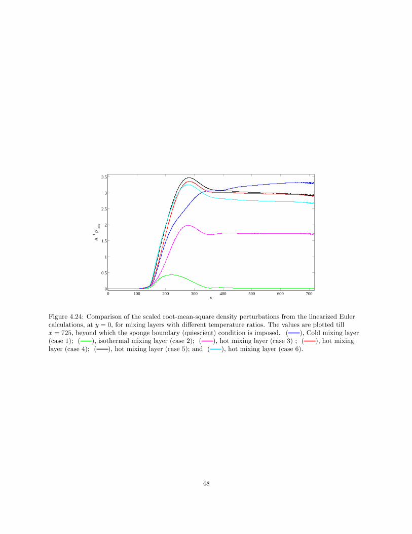
0 100 200 300 400 500 600 7000

0.5

1

1.5

2

2.5

3

3.5

x

A−

1 ρ′ rm

s

Figure 4.24: Comparison of the scaled root-mean-square density perturbations from the linearized Eulercalculations, at y = 0, for mixing layers with different temperature ratios. The values are plotted tillx = 725, beyond which the sponge boundary (quiescient) condition is imposed. ( ), Cold mixing layer(case 1); ( ), isothermal mixing layer (case 2); ( ), hot mixing layer (case 3) ; ( ), hot mixinglayer (case 4); ( ), hot mixing layer (case 5); and ( ), hot mixing layer (case 6).

48

4.3 Combining Linearized Euler Simulations and Linear Stability Theory

4.3.1 Amplitude of the instability wave

To understand the observations and compute the amplitude of the instability, we combine the results obtained

frommultiscale linear theory and from the linearized Euler calculations. We know the scaled root mean square

pressure perturbation, p′, from the simulations and eigenfunction, ζ, as well as eigenvalue, α, and phase

function, θ, from the linear theory. Using the expression in equation (2.55), we can now determine Aoeiθ at

y = 0 as shown in figure 4.25 by dividing the values of pressure perturbation with the eigenfunction at every

x-location. The ratio of the maximum value of Aoeiθ at y = 0 for the cold mixing layer to the maximum value

of Aoeiθ at y = 0 for the mixing layers of all the temperature ratios is = {1, 1.133, 1.243, 1.468, 1.630, 1.696}

respectively for cases 1 to 6.

49

0 100 200 300 400 500 600 7000

0.1

0.2

0.3

0.4

0.5

0.6

0.7

x

|Ao*

e(iθ)

|

Figure 4.25: Comparison of |Aoeiθ| at y = 0 for mixing layers with different temperature ratios. The valuesare plotted till x = 725, beyond which the sponge boundary (quiescient) condition is imposed. ( ), Coldmixing layer (case 1); ( ), isothermal mixing layer (case 2); ( ), hot mixing layer (case 3) ; ( ),hot mixing layer (case 4); ( ), hot mixing layer (case 5); and ( ), hot mixing layer (case 6).

Again mutliplying Aoeiθ by exp−iθ we get the amplitude of the instability wave as shown in figure 4.26,

where a log plot of the amplitude is presented. It is observed that the amplitude of the instability wave also

decreases with increase in temperature ratio. The amplitude is constant in the region where the mixing layer

is parallel with a zero spreading rate. In the unstable region, the wave grows rapidly and as the shear layer

thickness increases, the wave reaches its peak followed by a rapid decay in the stable region of the mixing

layer. It is observed that the growth rate of the wave is lowest for the cold mixing layer and increases with

increase in heating. This is consistent with the eigenvalue as shown in figure 4.1. Also, as expected the

location of the peak value of the instability wave moves upstream with heating which again is consistent

with the location of neutral stability moving upstream with heating from the linear stability analysis.

4.3.2 Directivity of the radiated sound

The directivity of the sound radiated is computed using the procedure mentioned in section 3.2.3. By

taking the Fourier transform of Ao exp iθ, we get go(k), where k is the wavenumber spectrum (which is

broadband), of the instability wave. Only those wavenumber components that correspond to the supersonic

phase velocity radiate sound into the far-field. Solving for directivity using equation (2.84) and considering

only those components in the wavenumber spectrum that radiate sound, we observe in figure 4.33 that the

sound radiated becomes quieter with heating. The peak radiation for the mixing layer increases by a small

amount with heating and it also seen that it becomes less directional for the hot mixing layers. This is

consistent with the results from [44]. The sound radiation decreases with increase in θ for all the cases after

50

0 100 200 300 400 500 600 700

−14

−13

−12

−11

−10

−9

−8

−7

−6

−5

x

log 10

(Ao)

Figure 4.26: Comparison of the amplitude of the instability wave in a log scale, log10|Ao|, at y = 0, formixing layer with different temperature ratios. ( ), Cold mixing layer (case 1); ( ), isothermalmixing layer (case 2); ( ), hot mixing layer (case 3) ; ( ), hot mixing layer (case 4); ( ), hotmixing layer (case 5); and ( ), hot mixing layer (case 6).

the peak radiation, except for case 6 with static temperature ratio of 2.75. For this case, it is seen that after

the peak at θ = 16.4, there is another peak of radiation at θ = 96.37°as shown in figure 4.34. The reason for

this second peak is not known yet. In the tables 4.2 and 4.3, only the first peak is used for comparison.

From equation (2.84), we see that D(θ) is proportional to |go(k)|2, which in turn is proportional to |p′|2in the far-field as r�∞. We therefore compare the ratio of peak value D(θ) of all the mixing layer cases

to that of the cold mixing layer case with the ratio of |p′|2 of all the cases to the cold mixing layer case

(table 4.2). To obtain this comparison, we trace the radiation path, as seen in figures 4.13 to 4.18 and

compute xint, the point where the radiation line intercepts the x−axis. From this x−intercept, we compute

the coordinates (xr, yr) of a point which is at a distance r = 380 (any large value of r can be chosen, since

the analytical expression for D(θ) was computed using stationary phase method where r�∞) along the

radiation direction). At this point (xr, yr), the ratio of |p′|2 from the linearized Euler simulations for (case

1)/(case *) is computed where ∗ represents all the cases from 1 to 6, respectively. A similar comparison is

given in table 4.3 where the value of r is taken as 250. The directivity as obtained from theory compares

well with the values from simulation. It is observed from the ratio of the amplitude of D(θ) that the sound

radiated in the far-field decreases with increase in heating. The intensity of sound radiated by the cold

mixing layer is higher than the intensity of sound radiated by the hot mixing layer (case 5) by a roughly a

factor of 15.

51

0 100 200 300 400 500 600 7000

2

4

6

8

10

12x 10

−6

x

Ao

Figure 4.27: Amplitude (Ao) of the instability wave at y = 0 for the cold mixing layer (case 1) with statictemperature ratio = 0.75. The location of peak amplitude at x = 219

100 200 300 400 500 600 7000

2

4

6

8

10

12

14

16x 10

−7

x

Ao

Figure 4.28: Amplitude (Ao) of the instability wave at y = 0 for the isothermal mixing layer (case 2) withstatic temperature ratio = 1.00. The location of peak amplitude at x = 216

52

100 200 300 400 500 600 700

0.5

1

1.5

2

2.5

3

x 10−7

x

Ao

sl2 TR = 1.247

Figure 4.29: Amplitude (Ao) of the instability wave at y = 0 for the hot mixing layer (case 3) with statictemperature ratio = 1.25. The location of peak amplitude at x = 207

100 200 300 400 500 600 7000

5

10

15x 10

−9

x

Ao

Figure 4.30: Amplitude (Ao) of the instability wave at y = 0 for the hot mixing layer (case 4) with statictemperature ratio = 1.75. The location of peak amplitude at x = 187

53

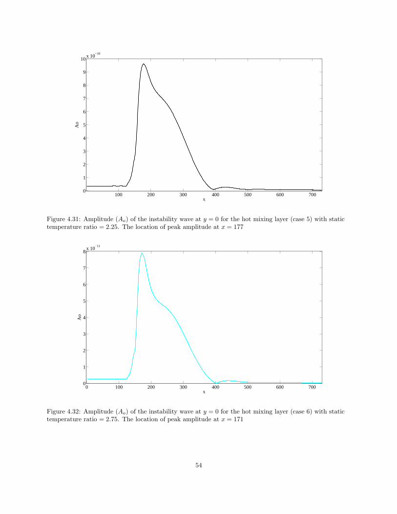
100 200 300 400 500 600 7000

1

2

3

4

5

6

7

8

9

10x 10

−10

x

Ao

Figure 4.31: Amplitude (Ao) of the instability wave at y = 0 for the hot mixing layer (case 5) with statictemperature ratio = 2.25. The location of peak amplitude at x = 177

0 100 200 300 400 500 600 7000

1

2

3

4

5

6

7

8x 10

−11

x

Ao

Figure 4.32: Amplitude (Ao) of the instability wave at y = 0 for the hot mixing layer (case 6) with statictemperature ratio = 2.75. The location of peak amplitude at x = 171

54

Table 4.2: Comparison of ratio of peak directivity with ratio of |p′|2 for the cold mixing layer case to themixing layer cases 1 to 6 taking r = 380.

case* x-int (xr,yr) |p′(case0)|2/|p′(case∗)|2 dir(case0) /dir(case∗)case 0 174.3 (525,145) 1.00 1.00case 1 174.6 (525,146) 1.89 1.89case 2 175.1 (526,147) 3.15 3.15case 3 174.6 (525,148) 7.95 7.93case 4 166.4 (521,136) 16.07 15.07case 5 165.9 (521,137) 29.80 22.93

Table 4.3: Comparison of ratio of peak directivity with ratio of |p′|2 for the cold mixing layer case to themixing layer cases 1 to 6 taking r = 250.

case* x-int (xr,yr) |p′(case0)|2/|p′(case∗)|2 dir(case0) /dir(case∗)sl0 174.3 (405,95) 1.00 1.00sl1 174.6 (405,95) 1.89 1.89sl2 175.1 (405,95) 3.28 3.15sl3 174.6 (405,95) 9.12 7.93sl4 166.4 (405,95) 20.67 15.07sl5 165.9 (405,95) 37.56 25.40

10 15 20 25 30 35 40 45 500

0.5

1

1.5

2

2.5

3

3.5

4

4.5

5x 10

−9

θ

D(θ

)

Figure 4.33: Comparison of directivity, (D(θ)), in the acoustic field for the mixing layer with differenttemperature ratios. ( ), Cold mixing layer (case 1) with maxD(θ) = 5× 10−9 at θ = 15.5; ( ),isothermal mixing layer (case 2) with maxD(θ) = 2.63× 10−9 at θ = 15.28; ( ), hot mixing layer (case3) with maxD(θ) = 1.59× 10−9 at θ = 15.23; ( ), hot mixing layer (case 4) withmaxD(θ) = 6.296× 10−10 at θ = 15.14; ( ), hot mixing layer (case 5) with maxD(θ) = 3.312× 10−10 atθ = 15.63; and ( ), hot mixing layer (case 6) with maxD(θ) = 5.765× 10−10.

55

0 50 100 1500

0.5

1

1.5

2

2.5

x 10−10

θ

D(θ

)

Figure 4.34: Directivity, (D(θ)), in the acoustic field for the hot mixing layer (case 6). The radiation peaksat θ = 96.37°where max(D(θ)) = 2.8× 10−10. The first peak occurs at θ = 16.22°with D(θ) = 2.181× 10−10.

56

CHAPTER 5

CONCLUSION

A planar, two-dimensional, high-speed mixing layer was analysed using linear stability theory and linearized

Euler calculations to study effect of heating on the dynamics of the large-scale structures and their associated

acoustic-field.

The spreading of the mean flow of the mixing layer leads to growth and decay of the instability wave,

which further leads to sound radiation from the instability wave. Using multiple scale expansion with the

expansion parameter as small as the spreading rate of the mixing layer, the linearized Euler equations are

reduced to an eigenvalue problem involving a second order ordinary differential equation and two boundary

conditions. The shooting method is implemented to solve for the eigenvalue. However, at the points where

the phase velocity of the instability wave is equal to the mean flow velocity, a mathematical singularity called

the critical point arises. In order to avoid this critical layer, the differential equation was mapped into a

complex plane and integrated using a mapping function. After computing the eigenvalues, the eigenfunction

was computed in a second step. Two approaches were taken in determining the eigenfunction. First involves

combining finite-difference method and method of Frobenius analysis near the critical point and (ii) second

method involves integrating along the real axis and deforming the path of integration very close to the

critical point. It is found that the eigenfunctions obtained from both methods are approximately equal with

in both the unstable as well as the stable region. This agreement in the two methods for computation of

the eigenfunctions has been verified only for the isothermal case but it confirms the methodology used to

compute accurately the eigenvalue and the eigenfunction in the damped region of the mixing layer.

From the linear stability analysis, we observed from the eigenvalue plots that the growth rate of the

instability wave increases with increase in heating and the neutral stability point moves upstream with

heating. This observation was consistent with the amplitude of the instability wave obtained by combining

results from the simulations and the linear stability theory. The amplitude of the instability wave also

decreases with increase in heating. Consistent with the experimental results, we observe that the acoustic

radiation in the far-field decreases with increase in heating from the directivity values. The cause for the

reduction is believed to be related to significant entropy fluctuations within the mixing layer created by

spatially varying mean velocity and mean entropy gradients.

To conclude, a mathematical procedure developed by Tam in [3] was extended to include the temperature

effects and study the effect of heating on sound radiated in the far-field. Frobenius method and complex

detour method, both can be used to determine the eigenfunction in the damped region of the mixing layer.

Using the first order approximation, we can approximately determine the amplitude of the instability wave

and the directivity by combining linear stability theory and data from linearized Euler calculations. The

consistent trends in results from both the simulation and the theory confirms again that as we increase the

57

temperature of the mixing layer, the sound radiated decreases and the instability wave plays an important

role in the sound radiation for high speed mixing layers.

5.1 Future Work

Currently, the instability wave solution is determined by combining both, the theory and simulation results.

The solution can also be computed using the theoretical expressions derived in chapter 2 and compared

with the solution from simulations. In the computation of the integrals (2.52) and (2.53) in the damped

region, the same deformed contour should be used to compute the integral as that used in computation

of the eigenfunction to avoid discontinuity at the critical point. The next step would be to compute the

amplitude of the instability wave from theory and compare it with the instability wave amplitude computed

by coupling the eigenfunction and linearized Euler simulation data.

The present analysis was carried out for a single frequency ω = 0.1. This can be extended further to

study the effect of frequency on spatially developing instability wave and its associated sound field. Further,

it will be interesting to use the numerical procedure to study the sound radiation for a subsonic mixing layer

to make the analysis complete.

This study and understanding of the dynamics of the large-scale structures in two-dimensional mixing

layers can be extended to understand the effect of heating on jet noise as well as methods to reduce the noise

radiated.

58

CHAPTER 6

REFERENCES

[1] T.Kelly and J.Allan, The Ecology of Transportation : Managing Mobility for the Environment. SpringerNetherlands, 2006.

[2] H. Hubbard, Aeroacoustics of Flight Vehicles: Theory and Practice. Volume 1: Noise Sources.Scientific and Techn. Information Office, Nat. Aeronautics and Space Administration, 1991, no. v. 1-2.[Online]. Available: http://books.google.com/books?id=PY06AQAAIAAJ

[3] C. Tam and P. Morris, “The radiation of sound by the instability waves of a compressible plane turbulentshear layer,” Journal of Fluid Mechanics, vol. 98, no. 02, pp. 349–381, 1980.

[4] C. Tam and D. Burton, “Sound generated by instability waves of supersonic flows. part 1. two-dimensional mixing layers,” Journal of Fluid Mechanics, vol. 138, no. 1, pp. 249–271, 1984.

[5] C. Tam and D. Burton, “Sound generated by instability waves of supersonic flows. part 2. axisymmetricjets,” J. Fluid Mech, vol. 138, no. 1, pp. 273–295, 1984.

[6] M. Lighthill, “On sound generated aerodynamically. i. general theory,” Proceedings of the Royal Society

of London. Series A. Mathematical and Physical Sciences, vol. 211, no. 1107, pp. 564–587, 1952.

[7] C. Ho and P. Huerre, “Perturbed free shear layers,” Annual Review of Fluid Mechanics, vol. 16, no. 1,pp. 365–422, 1984.

[8] J. BELL and R. MEHTA, “Development of a two-stream mixing layer from tripped and untrippedboundary layers,” AIAA journal, vol. 28, no. 12, pp. 2034–2042, 1990.

[9] C. K. W. Tam, “Directional acoustic radiation from a supersonic jet generated by shear layer instability,”Journal of Fluid Mechanics, vol. 46.

[10] “On the noise of a nearly ideally expanded supersonic jet,” J. Fluid Mech, vol. 51, no. 1, pp. 69–95,1972.

[11] K. Bishop, J. Williams, and W. Smith, “On the noise sources of the unsuppressed high-speed jet,”Journal of Fluid Mechanics, vol. 50, no. 01, pp. 21–31, 1971.

[12] P. Morris, “Flow characteristics of the large scale wave-like structure of a supersonic round jet,” Journal

of Sound and Vibration, vol. 53, no. 2, pp. 223–244, 1977.

[13] D. McLaughlin, G. Morrison, and T. Troutt, “Experiments on the instability waves in a supersonic jetand their acoustic radiation,” Journal of Fluid Mechanics, vol. 69, no. 01, pp. 73–95, 1975.

[14] D. McLaughlin, G. Morrison, and T. Troutt, “Reynolds number dependence in supersonic jet noise,”AIAA Journal, vol. 15, pp. 526–532, 1977.

[15] T. Troutt and D. McLaughlin, “Experiments on the flow and acoustic properties of a moderate-reynolds-number supersonic jet,” Journal of Fluid Mechanics, vol. 116, no. 1, pp. 123–156, 1982.

59

[16] G. Brown and A. Roshko, “On density effects and large structure in turbulent mixing layers,” Journal

of Fluid Mechanics, vol. 64, no. 04, pp. 775–816, 1974.

[17] D. Papamoschou and A. Roshko, “The compressible turbulent shear layer: an experimental study,”Journal of Fluid Mechanics, vol. 197, no. 1, pp. 453–477, 1988.

[18] A. Michalke, “Survey on jet instability theory,” Progress in Aerospace Sciences, vol. 21, pp. 159–199,1984.

[19] L. Lees and C. Lin, “Investigation of the stability of the laminar boundary layer in a compressible fluid,”1946.

[20] C. Lin, “On the stability of the laminar mixing region between two parallel streams in a gas,” DTICDocument, Tech. Rep., 1953.

[21] W. Blumen, “Shear layer instability of an inviscid compressible fluid,” Journal of Fluid Mechanics,vol. 40, no. 04, pp. 769–781, 1970.

[22] E. Reshotko, “Boundary-layer stability and transition,” Annual Review of Fluid Mechanics, vol. 8, no. 1,pp. 311–349, 1976.

[23] S. Maslowe, “Critical layers in shear flows,” Annual review of fluid mechanics, vol. 18, no. 1, pp. 405–432,1986.

[24] J. Boyd, “Complex coordinate methods for hydrodynamic instabilities and sturm-liouville eigenproblemswith an interior singularity,” Journal of Computational Physics, vol. 57, no. 3, pp. 454–471, 1985.

[25] A. Gill and G. Sneddon, “Complex mapped matrix methods in hydrodynamic stability problems,”Journal of Computational Physics, vol. 122, no. 1, pp. 13–24, 1995.

[26] P. Schmid and D. Henningson, Stability and transition in shear flows. Springer Verlag, 2001, vol. 142.

[27] E. Brambley, M. Darau, and S. Rienstra, “The critical layer in linear-shear boundary layers over acousticlinings,” submitted to Journal of Fluid Mechanics, 2011.

[28] F. Golanski, V. Fortune, and E. Lamballais, “Noise radiated by a non-isothermal, temporal mixinglayer,” Theoretical and Computational Fluid Dynamics, vol. 19, no. 6, pp. 391–416, 2005.

[29] D. Bodony and S. Lele, “On using large-eddy simulation for the prediction of noise from cold and heatedturbulent jets,” Physics of Fluids, vol. 17, p. 085103, 2005.

[30] D. Bodony and S. Lele, “Low-frequency sound sources in high-speed turbulent jets,” Journal of Fluid

Mechanics, vol. 617, no. 1, pp. 231–253, 2008.

[31] J. Panda and R. Seasholtz, “Experimental investigation of density fluctuations in high-speed jets andcorrelation with generated noise,” Journal of Fluid Mechanics, vol. 450, pp. 97–130, 2002.

[32] J. Panda, “Experimental investigation of turbulent density fluctuations and noise generation from heatedjets,” Journal of Fluid Mechanics, vol. 591, pp. 73–96, 2007.

[33] C. Hunter, J. Bridges, and A. Khavaran, “Assessment of current jet noise prediction capabilities,” 2008.

[34] G. Lilley, “The radiated noise from isotropic turbulence with applications to the theory of jet noise,”Journal of sound and vibration, vol. 190, no. 3, pp. 463–476, 1996.

[35] S. Pope, Turbulent flows. Cambridge university press, 2000.

[36] P. A.Thompson, Compressible Fluid Dynamics. New York NY:McGrawHill, 1972.

60

[37] M. Van Dyke, Perturbation methods in fluid mechanics. Parabolic Press Stanford, California, 1975,vol. 9.

[38] C. M. Bender and S. A. Orszag, Advanced Mathematical Methods for Scientists and Engineers: Asymp-

totic. Springer, Oct. 1999.

[39] D. Bodony, “Analysis of sponge zones for computational fluid mechanics,” Journal of Computational

Physics, vol. 212, no. 2, pp. 681–702, 2006.

[40] B. Strand, “Summation by parts for finite difference approximations for d/dx,” Journal of Computa-

tional Physics, vol. 110, no. 1, pp. 47–67, 1994.

[41] M. Svard, M. Carpenter, and J. Nordstrom, “A stable high-order finite difference scheme for the com-pressible navier–stokes equations, far-field boundary conditions,” Journal of Computational Physics,vol. 225, no. 1, pp. 1020–1038, 2007.

[42] D. Bodony, “Accuracy of the simultaneous-approximation-term boundary condition for time-dependentproblems,” Journal of Scientific Computing, vol. 43, no. 1, pp. 118–133, 2010.

[43] J. Bridges and M. Wernet, “Measurements of the aeroacoustic sound source in hot jets,” AIAA paper,vol. 3130, p. 2003, 2003.

[44] A. Sharma and S. Lele, “Effect of heating on noise radiation of a two-dimensional mixing layer: directcomputation and acoustic analogy predictions,” AIAA conference.

61