2012 ipl residential peer comparison em&v reportv report 2012 ipl residential peer comparison...
TRANSCRIPT

2012 IPL Residential Peer Comparison EM&V Report
July 11, 2013
FINAL
Prepared for
One Monument Circle
Indianapolis, Indiana 46206
Submitted by the TecMarket Team:
TecMarket Works, Opinion Dynamics, The Cadmus Group, Integral Analytics and Building Metrics
with Maria Larson

IPL Residential Peer Comparison EMV Report FINAL_clean.docx Page i
TABLE OF CONTENTS
1. IPL PEER COMPARISON PROGRAM EM&V RESULTS ......................................... 3
1.1 Program Description ................................................................................................................... 3
1.2 Scorecard and Evaluated Summary .......................................................................................... 4
1.3 EM&V Methodology Overview ..................................................................................................... 4
1.4 Impact Evaluation Results ........................................................................................................ 14
1.5 Cost-Effectiveness Analysis ...................................................................................................... 18
1.6 Program Insights and Implementation .................................................................................... 23
A. APPENDIX A: FIXED EFFECTS MODEL (DM VS. DM/EMAIL HOUSEHOLDS) .......... 25
B. APPENDIX B: FIXED EFFECTS MODEL OUTPUT FOR OVERALL PROGRAM .............. 29
C. APPENDIX C: COST EFFECTIVENESS DETAIL TABLES ....................................... 33
D. APPENDIX D: COMPARISON OF SAVINGS ESTIMATES FOR BEHAVIORAL PROGRAMS ACROSS THE COUNTRY ............................................................................. 35

IPL Residential Peer Comparison EMV Report FINAL_clean.docx Page ii
TABLE OF TABLES
Table 1: 2012 Peer Comparison Program Performance Goals ................................................................ 4
Table 2: Overall Program Evaluation Tasks ................................................................................................ 5
Table 3: Distribution of Report Start Date .................................................................................................. 9
Table 4: Fixed Effects Model Estimate of Overall Program Impacts: Dependent Variable is kWh/day (January 2010 to March 2013) ................................................................................................................. 10
Table 5: Fixed Effects Model Estimate of DM and DM/Email Impacts: Dependent Variable is kWh/day (January 2010 to March 2013) ................................................................................................................. 11
Table 6: Difference in Difference Estimator ............................................................................................. 13
Table 7: Participation Lift ........................................................................................................................... 14
Table 8: Difference in Difference in Savings ............................................................................................ 14
Table 9: Savings Adjustment ..................................................................................................................... 14
Table 10: IPL Peer Comparison Program Adjusted Net Savings for March 2012-February 2013 Program Period ........................................................................................................................................... 15
Table 11: Net Savings Adjustment ............................................................................................................ 15
Table 12: Reported Savings versus Evaluated Energy Savings .............................................................. 16
Table 13: Distribution of Report Start Date ............................................................................................. 17
Table 14: Confidence Interval: Dependent Variable is kWh/day (January 2010 to March 2013) ....... 18
Table 15: Estimated Impacts from Home Energy Reports ...................................................................... 18
Table 16: Cost-Effectiveness Test Overview ............................................................................................ 20
Table 17: Cost-Effectiveness Test Overview ............................................................................................ 20
Table 18: Cost-Effectiveness Results ....................................................................................................... 23
Table 19: Fixed Effects Model Coefficients .............................................................................................. 27
Table 20: Fixed Effects Model Coefficients for Overall Program ............................................................ 30

IPL Residential Peer Comparison EMV Report FINAL_clean.docx Page 3
1. IPL PEER COMPARISON PROGRAM EM&V RESULTS
Indianapolis Power and Light Company (IPL) is delivering Demand Side Management (DSM) programs to its customers. These programs are classified as “CORE” and “Core Plus” programs. CORE programs are delivered by a statewide Third-Party Administrator (“TPA”). Core Plus programs are programs that are in addition to IPL’s CORE Programs. This evaluation report focuses on one of IPL’s Core Plus efforts in 2012, namely the Residential Peer Comparison Energy Report program (“Peer Comparison program”).
The DSM Oversight Board and IPL contracted with the TecMarket Works (“TecMarket”) team to conduct an impact evaluation of the Peer Comparison program.
1.1 PROGRAM DESCRIPTION IPL designed a behavioral program, formally referred to as the Residential Peer Comparison program. According to the program staff, the main goal of this program is to significantly increase customer engagement across programs targeted within the IPL service territory for the purposes of:
1. Large-scale, measurable and cost-effective energy savings, over a three-year period 2. Increased program participation in select IPL Energy Efficiency, Renewables and Demand
Response programs 3. Increased customer satisfaction through an improved customer experience and engagement
The program uses behavioral science-based marketing to provide customized energy consumption information to selected IPL residential households. Treated households receive information on their energy consumption as compared to their peers with the theory that such comparisons will prompt measurable energy savings among treated households. The treated households receive a printed and mailed quarterly energy report. The report contains customized suggestions for reducing energy consumption.
The program aims to use an experimental design approach, namely a randomized control trial (RCT) design, to assign customers to the treatment and control groups. In an RCT, a target population is randomly assigned to treatment and control groups. Due to the randomization process, treatment and control group customers are theoretically “equivalent” and therefore any difference between the treatment and control groups’ energy use after receiving treatment is considered attributable to the treatment intervention.
The IPL Peer Comparison program was launched in March 2012. The program targets high-usage households that fall within the top 60% of high energy usage in the residential sector.
There were 26,855 high-usage (relative energy consumption) customers in the treatment group for the program, all of whom receive a quarterly energy report via mail. OPOWER, the program’s implementer, has email contact information for 7,690 customers within this treatment group. Thus, these customers also receive monthly email reports. All treatment customers have access to a web portal that contains the same information as in the reports.

IPL Residential Peer Comparison EMV Report FINAL_clean.docx Page 4
1.2 SCORECARD AND EVALUATED SUMMARY For 2012, IPL had a goal of delivering 6,120 MWh and 750 kW in net savings from the IPL Peer Comparison program. According to the scorecard, IPL reports that the program met a 100% of the participation goals, about three-quarters (77%) of the 2012 energy savings goals and 47% of demand goals (as reported, non-coincident peak). Overall, IPL spent 77% of the total implementation budget. Table 1 lists the goals associated with the Peer Comparison program.
Table 1: 2012 Peer Comparison Program Performance Goals
Planning
Goal (a) Reported(a) % of Goals
Number of Participants 25,000 25,000 100%
Budgets $381,000 $292,941 77%
Net kWh 6,120,000 4,724,000(b) 77%
kW 750 351 47% (a) Source: IPL 2012 Scorecard as of December 31, 2012 (b) Reported by IPL to reflected reported values for 10-month program period through December
2012 (reported values in the scorecard were for a 6-month period) Please note that the IPL scorecard is a calendar year based scorecard (reporting program performance from January through December 2012). The Peer Comparison program started accumulating savings in March 2012. Therefore, the reported savings in the scorecard are from March 2012 through December 2012 only. For purposes of this evaluation, we looked at a full 12-month period (March 2012 – February 2013) both due to regulatory requirements as well as to provide annual savings estimates for planning purposes. However, to be able to directly compare results to the 10-month reported savings in the scorecard, we report energy and demand savings in two ways:
• Savings for the 10-month 2012 period (March 2012 - December 2012), used to calculate a realization rate against the reported savings
• Savings for a 12-month period since program launch (March 2012 – February 2013), per regulatory requirements and to provide an annual savings estimate for planning purposes
1.3 EM&V METHODOLOGY OVERVIEW In this section, we provide a short description of the methods of data collection and analysis.
The evaluation efforts, per IPL’s request, are tailored to primarily address program net savings and cost-effectiveness, and they rely on the industry standard for data collection and analytical methods for evaluation measurement and verification (EM&V) of behavioral programs. As such, with the exception of discussions with the program manager to understand program parameters, and follow-up discussions with implementers, the EM&V activities do not include a process evaluation component.
Table 2 provides program specific EM&V activities performed by the TecMarket Team for the Peer Comparison program.

IPL Residential Peer Comparison EMV Report FINAL_clean.docx Page 5
Table 2: Overal l Program Evaluation Tasks Action Detai ls
Interviews with program managers and implementers
• Interviewed program managers and implementers to discuss program theory and implementation
Review tracking databases and select program materials
• Reviewed program databases and customers’ profiles for treatment and control population, identifying and addressing adjustments where required
Equivalency check analysis • Conducted the randomization of the treatment and control group customers ensuring that both groups are equivalent
Impact evaluation
• Conducted a billing analysis to quantify the energy saved through actions taken among the treatment compared with control group members
• Conducted a channeling analysis to calculate participation lift as well as remove any double-counting of savings from participation in other IPL programs
Cost-effectiveness analysis
• Collected program cost information • Using estimated load impacts and IPL’s data on avoided costs, rates,
and discount rate, employed the DSMore model to evaluate the cost-effectiveness of the program with respect to the Utility Cost test and the Total Resource Cost test
Each of the evaluation tasks are briefly summarized below and apply to the evaluation efforts associated with the Peer Comparison program.
1. Interview with Program Managers and Implementers: The TecMarket Team conducted interviews with program managers and implementers to obtain a detailed level of knowledge about the program. These interviews allowed the building of knowledge of general operational systems and procedures of the program, and provided additional information on the design and operations of these systems at a level of detail needed to conduct an impact evaluation.
2. Review Tracking Databases and Program Materials: We reviewed program tracking information for other IPL Core Plus programs and related CORE programs (managed statewide through Energize Indiana) as part of the channeling analysis. We also reviewed the billing data as part of the data input files that enable calculation of savings for this program, and made adjustments as necessary.
3. Equivalency Analysis: The TecMarket Team performed the randomization of the target population into treatment and control groups for the Peer Comparison program.
4. Impact Analysis: The impact evaluation quantifies the following:
• Evaluation of program net energy savings impact (billing analysis)
• Evaluation of double counting of savings in other IPL programs (channeling analysis)
Each of these is explained below.
a) Bil l ing Analysis with Control Group: Methods to calculate net impact provide the level of change in energy and/or demand due to the activities of the program. Given the experimental design and the use of a control group, the impact estimates are considered net savings and are calculated using billing data, frequently referred to as “billing analysis.” The control group represents energy consumption that would have occurred in the absence of the program. The benefit of this approach is that it accounts for interactive effects of multiple

IPL Residential Peer Comparison EMV Report FINAL_clean.docx Page 6
actions taken over time. For the purpose of conducting a billing analysis, we used the following data:
• Account and/or contact information, as well as the date actions were taken linked to the home where the energy reports were sent
• Treatment and a control group
• Pre-billing data (12 months of pre-program billing data)
• Post-billing data (12 months of billing data following program launch)
• Large sample sizes (to achieve sufficient statistical power to detect small effects)
This impact analysis relies on a Difference-in-Differences (DID) billing analysis of savings gained by the treatment group above the control group. Through this billing analysis, the TecMarket Team calculated net energy savings. However, this estimate includes other potential program effects, that is, savings that may have accrued if the treatment and control groups participated in other IPL CORE or Core Plus programs at different rates (e.g., more treatment than control customers participate in other programs). As such, a channeling analysis is used to estimate an adjustment factor to reduce the overall billing analysis estimates. This reduction is standard practice in behavioral program evaluations and is used to avoid double counting of other IPL CORE and Core Plus programs energy savings.
b) Channeling Analysis: The goal of conducting a channeling analysis is to quantify the savings that may be double-counted due to cross-participation in other programs. The savings tips provided in the reports, if effective, could lead to participation in other IPL CORE or Core Plus energy programs among program participants, and possibly a higher rate of participation among the treatment group compared to the control. Increased participation in other programs among the treatment participants would mean that some portion of savings achieved through these other programs may be attributable to some influence by the Peer Comparison program. However, since the savings are claimed by the other IPL programs, they should be removed from the Peer Comparison program (to avoid double counting). Through the channeling analysis, we develop an “adjusted net” savings value.
5. Cost-effectiveness Analysis: The TecMarket Team performed a cost-effectiveness analysis for the Peer Comparison program using the proprietary DSMore cost-effectiveness software, which is used in over 30 states and accepted by regulatory commissions throughout the country. Cost-effectiveness results help IPL understand the overall cost-effectiveness relative to the original goals established by the program planners. The conditions that influence participation, savings, avoided cost benefits, lost revenue and other program parameters are analyzed together in the cost-effectiveness ratios, thereby providing guidance and insights into improving program design and measure selection. Key decisions made for this analysis included the appropriate specification of regional weather zones, determination of the appropriate estimation of avoided future energy costs, determination of avoided transmission and distribution (T&D) values per region, regional losses, and other necessary modeling inputs used for valuation. The cost-effectiveness calculations use algorithms consistent with the Indiana Evaluation Framework and the California Standard Practice Manual (SPM), and adjusted for regional weather, price and load shape conditions, and region-specific impacts these factors have on program results. However, the Indiana Evaluation Framework takes precedence over the SPM when applicable. The results are reported for weather normal conditions, and the full range of weather conditions the program is likely to encounter. The results are analyzed on the program level (given that measure-level impact is not applicable for a Peer Comparison

IPL Residential Peer Comparison EMV Report FINAL_clean.docx Page 7
program). Reported outputs include pertinent information on program costs, load savings, avoided costs, life of measure savings, and capacity savings.
1.3.1 EQUIVALENCY CHECK ANALYSIS Given that the net savings for behavioral programs is contingent on the defensibility of the experimental design, the TecMarket Team randomly assigned 44,400 IPL target customers into a treatment (initially 27,750) and control group (initially 16,650) for the program on behalf of IPL in the first year of the program evaluation. The randomization was conducted four times and the groups were checked for equivalency. The program implementer, OPower, selected one of the four randomization schemes to guide delivery of the reports over the program period. As such, the treatment and control groups were deemed to be equivalent. Over time, the treatment and control groups experienced some natural attrition and other adjustments which, for purposes of this impact evaluation, reduced the treatment group number of customers to 26,855 and control customers to 16,102 (see Table 3 and discussion below in Section 1.3.2 Billing Analysis).
The program intends to expand the treatment group in 2013. For this purpose, the TecMarket Team also performed additional randomization for an expansion group of 65,000 treatment customers in the spring of 2013. The evaluation of this expansion group falls outside the scope of the 2012 EM&V effort.
1.3.2 BILLING ANALYSIS The TecMarket team conducted a billing analysis to assess changes in energy consumption attributable to the Peer Comparison program. This analysis relied upon a statistical analysis of monthly electricity billing data for all IPL customers who received the Home Energy Report (the treatment group) and a matched sample of customers that did not receive any information from the program implementer (the control group) as chosen through the randomization process. The terms of the model are further defined by whether customers received quarterly paper reports (DM households) or quarterly paper reports and monthly email reports (DM/email households)
This final impact evaluation used a Fixed-Effect (FE) panel regression model that controls for time-invariant differences across individual customers. Appendix A and Appendix B provide the detailed model specifications and results.
This model can be expressed as:
Equation 1: Fixed Effect Model – DM and DM/email Savings
𝑘𝑊ℎ!" = 𝛼! + 𝛼!𝑀𝑜𝑛𝑡ℎ𝐼𝐷! + 𝛼!𝐶𝐷𝐷!" + 𝛼!𝐻𝐷𝐷!" + 𝛽!𝑃𝑜𝑠𝑡!𝐸𝑚𝑎𝑖𝑙!!𝛽!𝑃𝑜𝑠𝑡!𝐷𝑀! + 𝛽!𝑃𝑜𝑠𝑡!𝑃𝑎𝑟𝑡!𝐷𝑀!+ 𝛽!𝑃𝑜𝑠𝑡!𝑃𝑎𝑟𝑡!𝐸𝑚𝑎𝑖𝑙! + 𝜀!"
The more relevant terms for evaluating program impact are:
1. Post*DM: It is a multiplication of the variable ‘Post’ and the variable ‘DM’. Post1 is a dummy variable which equals to one if the month is in the post-program period; 0 otherwise. DM is a
1 The very first month during which the first report was sent was deleted from the analysis. For example if the first report went out on March 9th within a billing period of March 1st – March 31st, March is considered “dead-band” and is excluded from the analysis. This is a consistent approach across the other Indiana utilities.

IPL Residential Peer Comparison EMV Report FINAL_clean.docx Page 8
categorical variable which equals to one where paper reports (DM) is the only treatment approach available for both treatment and control group members; 0 otherwise. ‘Post*DM’ measures during the post-program period how customers eligible for paper reports only changed their consumption (given email = 0).
2. Post*Email: It is a multiplication of the variable ‘Post’ and the variable ‘Email’. Email is a categorical variable which equals to one where email is available for both treatment and control group members, 0 otherwise. ‘Post*Email’ measures during the post-program period how customers eligible for email (in addition to paper reports) changed their consumption (given Email = 1). Note these consumption changes are NOT caused by the program because it is estimated based on treatment and control group members.
3. Post*Part*DM: it is a multiplication of the variable ‘Post’, ‘Part’ and the variable ‘DM’. Post as previously discussed tracks the post-program period. ‘Part’ is a dummy that tracks treatment group membership: i.e. Part equals to one if a customer is included in the treatment group, 0 otherwise. ‘Post*Part*DM’ measures during the post-program period how the report had changed the consumption of recipients who were eligible for paper reports only.
4. Post*Part*Email: it is a multiplication of the variable ‘Post’, ‘Part’ and the variable ‘Email’. Post as previously discussed tracks the post-program period. ‘Part’ is a dummy that tracks treatment group membership: i.e. Part equals to one if a customer is included in the treatment group, 0 otherwise. Post*Part tracks the treatment group membership during the post-program period; ‘Post*Part*Email’ measures during the post-program period how program treatment (paper report and email) changed the consumption of recipients who were eligible for email and paper reports.
Further description of the model and other terms in the model are presented in Appendix A.
In this equation, the effect of DM households is the coefficient on the Postt Parti 𝐷𝑀!variable (β1), and the incremental effect of the emailed reports (for DM/email households) is given by the coefficient on the Postt PartiEmaili variable (β2). Also, Post represents a dummy variable equal to one for data points after the first report has been sent and Part represents a dummy variable equal to one for participants and equal to zero for those in the control sample. The very first month during which the first report was sent was deleted from the analysis. For example if the first report went out on March 9th within a billing period of March 1st – March 31st, March is considered “dead-band” and is excluded from the analysis. This is a consistent approach across the other Indiana utilities.
The overall effect of the program is an average of DM effect and DM/email effect which is estimated by the model as:
Equation 2: Fixed Effect Model – Direct Overal l Savings
𝑘𝑊ℎ!" = 𝛼! + 𝛼!𝑀𝑜𝑛𝑡ℎ𝐼𝐷! + 𝛼!𝐶𝐷𝐷!" + 𝛼!𝐻𝐷𝐷!" + 𝛽!𝑃𝑜𝑠𝑡! + 𝛽!𝑃𝑜𝑠𝑡!𝑃𝑎𝑟𝑡! + 𝜀!"
In this model, the overall program treatment effect is captured by the coefficient on the term Postt Parti (β1). Definitions for all terms in this model are presented in Appendix B.
IPL Residential Peer Comparison EMV Report FINAL_clean.docx Page 9
Data Preparation
The data used in the billing analysis comes from three primary sources:
• Monthly billing data from January 20102 to March 2013, obtained directly from IPL;
• Weather conditions (temperature to calculate HDD and CDD) from the National Oceanic and Atmospheric Administration’s (NOAA’s) National Climatic Data Center (NCDC); and
• Program launch date specific to each customer (treatment and control) from OPower.
To develop the dataset used for the statistical analysis, the TecMarket Team conducted the following data processing steps:
• Determined the usage on a calendar month basis for each customer based upon their read cycle;
• Linked this usage data with the appropriate weather data, where a weather station was assigned based upon the distance between each weather station and the customer’s ZIP code;
• Linked the usage and weather data with the customer-specific program start date and whether or not the customer has email.
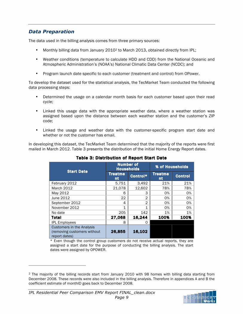
In developing this dataset, the TecMarket Team determined that the majority of the reports were first mailed in March 2012. Table 3 presents the distribution of the initial Home Energy Report dates.
Table 3: Distr ibution of Report Start Date
Start Date
Number of Households % of Households
Treatment Control* Treatme
nt Control
February 2012 5,751 3,492 21% 21% March 2012 21,078 12,602 78% 78% May 2012 6 3 0% 0% June 2012 22 2 0% 0% September 2012 4 2 0% 0% November 2012 1 1 0% 0% No date 205 142 1% 1% Total 27,068 16,244 100% 100% IPL Employees 8 0 Customers in the Analysis (removing customers without report dates)
26,855 16,102
* Even though the control group customers do not receive actual reports, they are assigned a start date for the purpose of conducting the billing analysis. The start dates were assigned by OPOWER.
2 The majority of the billing records start from January 2010 with 98 homes with billing data starting from December 2008. These records were also included in the billing analysis. Therefore in appendices A and B the coefficient estimate of monthID goes back to December 2008.

IPL Residential Peer Comparison EMV Report FINAL_clean.docx Page 10
The analysis eliminated treatment and control customers who did not have a start date in the program tracking data. Moreover another 8 homes were removed because they were identified as IPL employees. Thus, the following analysis consists of data from 42,957 households, of which 26,855 are in the treatment group (i.e., 27,068 minus 205, minus 8 IPL employees) and 16,102 are in the control group (i.e., 16,244 minus 142).
Analysis
Both models controlled for time-invariant differences across customers via the customer-specific constant term (the fixed-effect), weather (via HDD and CDD terms). The DM vs. DM/email savings model controlled for whether or not the customer had email during the post-treatment period.
The FE models use monthly kWh3 as the dependent variables and the pre-participation kWh was used as the denominator. The equivalent percentage savings were also calculated. In summary:
• The overall program impact was estimated to be 22.23 kWh/month/household savings, or approximately 266.86 kWh per year/household before channeling analysis adjustments. This equates to about 1.0% of the total annual kWh consumption.
• The program impact among DM households was estimated to be 24.4 kWh/month/household. It is divided by the pre-program usage of the DM households which was 2,234 kWh/month/household. The equivalent percentage saving = 24.4 /2,234 = 1.1%.
• The program impact among DM/email households was estimated to be 16.3 kWh/month/household. The DM/email pre-program usage was 1,952 kWh/month. The equivalent percentage saving = 16.3 / 1952 = 0.8%.
Table 4 and Table 5 present the estimated fixed effect regression models for the program overall as well as for the DM households vs. DM/email households impacts, respectively.
Table 4: Fixed Effects Model Estimate of Overal l Program Impacts: Dependent Variable is kWh/day (January 2010 to March 2013)
Variable
Coeff ic ient (Negative Values
= Saving) Per Part ic ipant
t -value Equivalent to Percentage
Impact: Post*Part -22.2379181 -9.01 -1.0% Post 17.0512717 2.01 NA HDD 2.5578770 291.63 NA CDD 4.4201823 123.97 NA Sample Size 1,657,335 rows (42,957 homes) R-Square 53%
3 The monthly kWh is the “calendarized” monthly kWh therefore the varying billing cycle has been adjusted.

IPL Residential Peer Comparison EMV Report FINAL_clean.docx Page 11
Table 5: Fixed Effects Model Estimate of DM and DM/Email Impacts: Dependent Variable is kWh/day (January 2010 to March 2013)
Variable
Coeff ic ient (Negative Values
= Saving) Per Part ic ipant
t -value Equivalent to Percentage
DM Impacts Only: Post* Part*DM -24.4106063 -8.38 -1.1%
DM/email Impact: Post* Part*Email -16.3170082 -3.51 -0.8%
Post*DM 7.4657165 0.87 NA Post*Email 39.6472875 4.40 NA HDD 2.5583490 291.70 NA CDD 4.4214674 124.01 NA Sample Size 1,657,335 rows (42,957 homes) R-Square 52%
Overall, the Peer Comparison program recipients achieved an unadjusted net savings of approximately 267 kWh per year per participant (before channeling adjustments). The 10-month planning goal as calculated through the scorecard is approximately 244 kWh / year per participant and the 10-month reported savings is approximately 119 kWh / year per participant. As such, the unadjusted impact estimate is more closely aligned with the planning assumptions.
See Section 1.4 Impact Evaluation Results for a detailed explanation of adjusted (final) impact values both for the program overall and for the DM vs. DM/email populations.
1.3.3 CHANNELING ANALYSIS The savings tips provided in the Home Energy Reports, if effective, could lead to participation in other IPL energy efficiency programs among program participants, or a higher rate of participation among the treatment group compared to the control. Increased participation in other IPL energy efficiency programs among the treatment participants would mean that some portion of savings from other programs may be counted by both the behavioral program (through the billing analysis savings estimate) and other IPL programs (through deemed savings in their tracking databases). The purpose of a channeling analysis is to answer the following two questions:
• Part ic ipation Lift : Does behavioral program treatment have an incremental effect on participation in other IPL energy efficiency programs?
• Savings Adjustment: What portion of savings from behavioral program treatment is double-counted by other IPL energy efficiency programs?
Thus, the objective of the savings adjustment component of channeling analysis is to determine what portion of savings detected in the billing analysis is also captured by other IPL Core Plus programs, and adjust savings to reflect only the “unique” component of savings directly attributable to the Peer Comparison program.
Participation Lift Analysis
To determine whether the Peer Comparison program treatment generates lift in other energy efficiency programs, the TecMarket Team calculated whether more treatment than control group members participated in other residential IPL DSM programs after the start of the Peer Comparison

IPL Residential Peer Comparison EMV Report FINAL_clean.docx Page 12
program. The TecMarket Team cross-referenced the databases of the behavioral program—both treatment and control groups—with the databases of other residential IPL CORE and Core Plus DSM programs available to the customer base targeted by the behavioral program. Other program databases cross-referenced include:
• Air Conditioning Load Management
• Energy Assessment (online kit)
• Energy Assessment Program
o Walk Through Assessment with Direct Install component, through December 2011)4
o CORE HEA program (beginning January 2012)
• High Efficiency HVAC Program
• Residential Renewables Incentives Program
• Second Refrigerator Pick-up and Recycling
Other Residential Core Plus programs were reviewed but not included in the analysis:
• New Construction: Rebates were given to builders of new homes. Customers at the new home, if part of the treatment group, received the Home Energy Report after they occupied their home; thus, their decision to move into an energy efficient home was not influenced by the Peer Comparison program
• Multifamily Direct Install (MFDI): The Peer Comparison program is geared towards single-family customers (although some multifamily addresses appear to be part of the treatment and control populations); further the MFDI tracking database contains property address, not individual customer records for tenants in the premises’ units, thus not allowing for linkages of records between Peer Comparison and multifamily program tracking databases
Program participation matching took into consideration dates of receipt of the Home Energy Reports and dates of participation in IPL Core Plus programs to establish whether the customers who participated in other programs were in the pre- or post-period.
Savings Adjustment Analysis
The savings accrued to Peer Comparison program participants are two-fold: energy savings through Peer Comparison behaviors or as a result of being channeled to other IPL CORE and Core Plus programs where they install (or recycle) measures that lead to energy savings. While the Peer Comparison program may have been the trigger for participation in other Core Plus programs, these savings are typically already claimed by the other programs. The objective of the savings adjustment is to determine what portion of net savings, as measured through the billing analysis, is captured in other program databases, and then to adjust net savings to reflect only direct savings obtained outside of other programs so that savings will not be double counted.
4 This program was a part of the Core Plus programs in 2011 but was moved to the CORE HEA programs in January 2012

IPL Residential Peer Comparison EMV Report FINAL_clean.docx Page 13
The starting point is program’s unadjusted net energy savings detected in the billing analysis. To estimate these savings, the TecMarket Team first estimates total net program savings from the billing analysis, and then estimates net channeled savings as the difference between savings from other programs achieved by the participant group, compared with the control group, to further refine net savings estimates.
To determine the net savings adjustment component of the channeling analysis, the TecMarket Team took the following steps:
Step 1: Overlap in units: Similar to the participation lift analysis, the TecMarket Team cross-referenced the database of the Peer Comparison program, both treatment and control groups, with the databases of other residential IPL CORE and Core Plus programs available during the same period.
Step 2: Evaluated savings of overlapping units: Once the overlapping units were established, the per-measure (per program) evaluated net deemed savings were applied to the units to get the kWh savings for both the pre- and post-program period for the treatment and control groups.
Step 3: Difference-in-difference approach: Using the difference-in-difference approach, the TecMarket Team used the net deemed savings to calculate the savings adjustments (see tables below).
Table 6: Difference in Difference Estimator
Pre Post Post-Pre Difference Treatment Y0t Y1t Y1t-Y0t Control Y0c Y1c Y1c-Y0c T-C Difference Y0t-Y0c Y1t-Y1c (Y1t-Y1c) - (Y0t-Y0c)
Step 4: Calculate per household adjustment: The savings adjustment values are then divided by the modeled baseline assumptions (as calculated in the billing analysis) to get the household level adjustment values.
Participation Lift Analysis Results
Through this database cross-referencing, the TecMarket Team determined whether each program household (both treatment and control groups) participated in any program after the household received the first report through the Peer Comparison program. The difference in treatment and control participation rates is the participation lift.
Overall, the treatment group customers have a higher rate of participation than the control group. Thus, there is participation lift. Specifically, the Peer Comparison program is producing an increase in participation both within the treatment group (comparing post-report and pre-report periods, there is an increase in participation by 0.57%) as well as between the treatment and control groups (post period compared to the pre period is higher for the participant group than for the control group by 0.46%, see Table 7). This participation lift analysis shows that the program is driving participation in other IPL CORE and Core Plus programs, that is, about 125 customers participated in IPL programs due to the Peer Comparison report’s influence.

IPL Residential Peer Comparison EMV Report FINAL_clean.docx Page 14
Table 7: Part ic ipation Lift
Program Name Treatment (Post-Pre)
Control (Post-Pre)
Difference-in-
Difference Residential Energy Assessment -0.81% -0.88% 0.07%* HVAC Efficiency Program 0.27% 0.24% 0.03% Residential Second Refrigerator Pick-up and Recycling 0.31% 0.24% 0.07% Residential Air Conditioning Load Management 0.03% -0.03% 0.06% Residential Walk Through Assessment and Direct Install 0.77% 0.54% 0.23% Residential Renewables Incentives 0.00% 0.00% 0.00% Total 0.57% 0.11% 0.46%
* The DID calculates the differences between the treatment and control groups. Thus, even though the individual participant lift for both the treatment and control groups is negative, the treatment group lift is still higher than the control group. As such, DID results in a positive participation lift.
Savings Adjustment Results
The result of this database cross-referencing and calculation is a channeled savings estimate, which is then subtracted from the estimate of total program savings, as these savings, as noted above, are already claimed by other programs. The adjusted savings reflect only the “unique” component of savings directly attributable to the Peer Comparison program.
Table 8: Difference in Difference in Savings
kWh Pre-treatment
Post-treatment
Post-Pre Difference
Treatment 32.57 22.39 (10.18) Control 29.76 18.73 (11.04) T-C Difference 2.81 3.66 0.86
The savings adjustment values were divided by the modeled baseline assumptions (25,848 kWh per treatment customer—as calculated in the billing analysis) to get the household level adjustment values.
Table 9: Savings Adjustment
kWh Pre-treatment
Post-treatment
Post-Pre Difference
Treatment 0.13% 0.09% -0.04% Control 0.12% 0.07% -0.04% T-C Difference 0.01% 0.01% 0.003%
1.4 IMPACT EVALUATION RESULTS This section provides the results from the impact analysis conducted by the TecMarket Team.
Net Energy Savings Impact

IPL Residential Peer Comparison EMV Report FINAL_clean.docx Page 15
Applying the adjusted savings to the impact estimates, the Peer Comparison program had a final adjusted program savings of 0.997% per household or 265.98 kWh / year per household (see Table 10 and Table 11).
Table 10: IPL Peer Comparison Program Adjusted Net Savings for March 2012-February 2013 Program Period
Segment Annual kWh Savings % Savings
Average Per Treatment Customer (before channeling analysis adjustment) 266.86 1.00%
Final Adjusted Net Savings 265.98 0.997%
Table 11: Net Savings Adjustment
Impact Estimates
Bi l l ing Analysis Impacts Net Program Savings (% per HH) 1.00% 90% Confidence Interval Lower Bound 0.8% 90% Confidence Interval Upper Bound 1.3% Net Program Savings (Delta kWh per HH) 266.86 kWh 90% Confidence Interval Lower Bound 209 kWh 90% Confidence Interval Upper Bound 325 kWh Channeling Adjustments Net Program Savings (Delta kWh) 0.88 Incremental Savings from Other Programs (% per HH) 0.003% Net Adjusted Impacts Final Adjusted Net Savings (% per HH) 0.997% Final Adjusted Net Savings (Delta kWh) 265.98 kWh
Overall, the program achieved a net adjusted savings of 7,143 MWh during a full year 12-month program period. In order to calculate realization rates, we established that the treatment customers in the program accrued 5,580 MWh in net energy savings through December 20125 with a realization rate of 1.18.
5 A fixed effect model was used to determine the savings through December 2012. The model included two variables, the first variable equals to one during the first 10 months for those treatment members, zero otherwise. The second variable equals to one after 2012 for treatment members, zero otherwise.

IPL Residential Peer Comparison EMV Report FINAL_clean.docx Page 16
Table 12: Reported Savings versus Evaluated Energy Savings
Audited Volume
Verif ied
Volume
Ex-ante (Scorecard) savings
for 10-months in
2012 (MWh)
Ex-post Net
Adjusted Savings
by Customer (kWh)
Ex-post Savings
(12 months) (MWh)
Ex-post Savings
annualized for 10-
months in 2012
(MWh) Realizatio
n Rate 25,000 26,855 4,724 265.98 7,143 5,580 1.18
When we compare IPL’s savings (as a percentage savings reduction) to those seen in other jurisdictions across the country, the established savings of 0.997% falls on the lower part of the range of savings estimated for similar programs. The absolute value of 266 kWh/household, however, is on the high end of the spectrum. These findings are due to the fact that the IPL program targets high-energy consumption homes, with a relatively high baseline. Appendix D shows a range of established savings levels for various behavioral programs across the nation as a benchmark. Notably based on analysis of similar programs in other jurisdictions, behavior programs tend to see a ramp-up effect (increased average savings per participant) as they move into the second year of implementation.
As mentioned above, the savings and conclusions of this analysis are based on the Peer Comparison program participant population which, by design, consisted of high-energy consumption users. The findings of this evaluation thus apply to this population only.
A note on demand savings
The IPL Peer Comparison Program reported demand savings in its scorecards. These demand savings can be defined as an average demand savings across the program period (calculated by dividing energy savings by the number of hours within the period when savings accrued).
It is typically more valuable to determine peak demand savings. However, peak demand values are hard and expensive to estimate as it requires large sample sizes and interval meter information applicable for the population. An alternate approach would be to use survey data and/or load factors for the population segment, but there is a great degree of uncertainty in this type of an estimate.
Given the complexity and expense associated with determining peak demand impacts from behavioral programs, very few studies have been done on this across the country. However, an in-depth study conducted for SMUD study established a peak coincident ratio for an OPOWER program. While we recognize that there are likely Indiana specific characteristics related to geography, socio-demographic information, weather patterns, etc., we refer to this study to provide a sense of the demand impacts from this program. The approach is documented in a report titled the “Impact & Persistence Evaluation Report on Sacramento Municipal Utility District Home Energy Report Program” published in November 2012. The established kW/kWh ratio relies on a battery of survey research that measures what actions the report recipient had adopted after receipt of the Home Energy Report. The survey data was combined with building simulation models to estimate end-use unit energy kWh and kW savings. This estimate was then calibrated to the kWh savings estimate from a billing analysis.
The SMUD study found a kW/kWh ratio of 0.000294 for coincident demand savings. While again, we do not believe this is directly applicable to the IPL service territory, should we apply this factor to the net adjusted overall annual program saving (265.98 kWh per year per participant) this would result in coincident demand savings of 0.0782 kW per participating customer. This would then in turn result into peak coincident savings of approximately 2,100 kW.

IPL Residential Peer Comparison EMV Report FINAL_clean.docx Page 17
Analysis of savings for DM vs. DM/email Households
This section discusses differences in observed savings from DM households, compared to DM/email households. It should be noted that these two groups are not statistically equivalent. The latter group provided email addresses to IPL, which is likely to be correlated with other characteristics which can interact with the treatment effect (e.g. unobserved attitudes, energy behaviors). Therefore, differences in treatment effect between the DM households and the DM/email households could be partially attributed to the moderating effects of these other factors, as well as the receipt of email reports in addition to paper. The fixed effects cannot eliminate the possibility of heterogeneous treatment effects due to these fixed factors.
In the future, an experiment could be designed in which customers that have provided email addresses to the utility are randomized into a control group, DM group and DM/email households group. Such an experiment would reveal the effect of adding email to the paper reports for customers who provide email addresses to the utility. The experiment in this report did not contain a group for customers that had provided email addresses but received paper-only.
Table 13: Distr ibution of Report Start Date
Start Date Number of Households DM DM/email
February 2012 4,003 1,748 March 2012 15,200 5,878 May 2012 0 6 June 2012 20 3 September 2012 4 0 November 2012 1 0 Total 19,228 7,635
In evaluations performed in other jurisdictions there are instances where the savings by the DM/email households exceed those of DM households.
The TecMarket Team used the same fixed effect modeling process with the difference that the overall participation variable was separated into two variables: one for tracking the post-program participation with email for those customers which had provided email address to IPL and another variable tracking the post-program participation with only the paper report – these are customers who had not provided email address to the utility. Detailed model specifications and results can be found in Appendix A.
While savings in the DM/email households were not statistically significantly different from DM households , this result should not be interpreted as evidence on the relative effectiveness of the treatments since the two groups were not statistically equivalent per the discussion above. Please note the following:
• DM/email households achieved average energy savings of 16 kWh/month per household (approximately 192 kWh/year).
• DM households achieved a saving of 24 kWh/month per household (approximately 288 kWh/year).
• Although the magnitude of impact from DM/email households seem to be different, this difference is not statistically significant nor can the difference be attributed to the different treatments since the characteristics of the two groups are different and therefore the

IPL Residential Peer Comparison EMV Report FINAL_clean.docx Page 18
treatment effect will vary based on the moderating effect of these factors as well.6 It is possible that the tracking database contains classifications on whether the customer signed up for paper only, or paper and email at the outset of the project or at a particular point in time, and this may have changed over time (customer may have commenced receiving email reports a time after they signed up for the program).
Table 14 shows that the energy saving from DM households range from 18 kWh/month up to 30 kWh/month. The DM/email households savings range from 7 kWh/month up to 25 kWh/month. The actual saving could be anywhere within this range.
Table 14: Confidence Interval: Dependent Variable is kWh/day (January 2010 to March 2013)
Variable Point Estimates Per Part ic ipant Lower Bound Upper Bound
DM households -24.41 -30.12 -18.70 DM/email households -16.32 -25.42 -7.21
Table 15 highlights the average annual savings for DM/email households and DM households as well as the confidence bounds around these point estimates. Note these findings do not reflect the relative effectiveness of the two treatments as the groups are not equivalent and the impact of paper reports for the DM/email households is likely to be different based on different underlying characteristics.
Table 15: Estimated Impacts from Home Energy Reports7
Segment Annual
kWh Savings
95% Confidence
Interval Bounds
% Savings
95% Confidence
Interval Bounds
Baseline Usage kWh
/year Lower Upper Lower Upper
DM Households 288 224 361 1.1% 0.8% 1.3% 26,808
DM/email households 192 87 305 0.8% 0.4% 1.3% 23,424
Average Per Treatment Customer 2678 209 325 1.0% 0.8% 1.3% 25,848
1.5 COST-EFFECTIVENESS ANALYSIS Cost-effectiveness analysis is a form of economic analysis that compares the relative costs and benefits of two or more courses of action. In the Energy Efficiency industry, it is an indicator of the energy supply relative performance or economic attractiveness of any energy efficiency investment or practice when compared to the costs of energy produced and delivered in the absence of such an investment, but without consideration of the value or costs of non-energy benefits or non-included externalities. The typical cost-effectiveness formula provides an economic comparison of costs and
6 No statistically significant difference means that the saving impact was estimated to be a range by the Fixed Effect model and this range (i.e., confidence interval) of email and paper reports overlapped. 7 The value and confidence levels for the written and electronic reports and the average across all treatment customers is based on taking linear combinations of the estimated coefficients for the treatment and treatment interacted with email variables presented later in the report. 8 Note that this number is from billing analysis. After adjusting for channeling analysis the average per treatment customer saved approximately 266 kWh per year.

IPL Residential Peer Comparison EMV Report FINAL_clean.docx Page 19
benefits. All of the tests are reported based upon the net-present value (NPV) of the benefits and costs.
Typically, the cost-effectiveness evaluation is conducted in accordance with the procedures specified in the Indiana Evaluation Framework (Framework). While, the cost-effectiveness approaches in the Framework follow the California Standard Practice Manual (SPM), the Indiana Evaluation Framework takes precedence over the SPM when applicable. Adherence to the procedures in the Framework and the SPM may follow a number of paths; but, two approaches are the most prevalent. One involves evaluating the ex-ante cost-effectiveness, i.e., the cost-effectiveness of proposed programs. The second involves evaluating energy efficiency programs on an ex-post basis. The ex-ante approach uses projected measure impacts, while the ex-post approach uses actual results from the evaluation, measurement, and verification process (as described in this report). This report uses the ex-post approach for the cost-effectiveness analysis which is consistent with the analysis requirements of the Indiana Evaluation Framework.
1.5.1 COST-EFFECTIVENESS MODEL DESCRIPTION EM&V and cost-effectiveness modeling are critical to the long-term success of energy efficiency programs. To understand cost-effectiveness, the utility/program administrator should have a model that can evaluate changes to both individual programs and a portfolio. This includes but is not limited to the ability to evaluate the impact on cost-effectiveness of changes in numerous factors such as: incentive levels, participant levels, measure savings, measure costs, avoided costs, end-use load shapes, coincident peak factors, net-to-gross factors, administrative costs, and the addition or deletion of measures or programs.
To provide the best and most accurate demand side management (DSM)/demand-response (DR)/energy efficiency portfolio cost-effectiveness modeling, the TecMarket team used the DSMore software (DSMore). DSMore captures hourly price and load volatility across multiple years of weather which is needed to assess the true cost-effectiveness of the programs under expected supply and load conditions, especially for extreme weather situations.
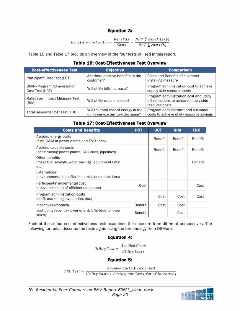
In its simplest form, energy efficiency cost-effectiveness is measured by comparing the benefits of an investment with the costs. There are five primary cost-effectiveness tests that may be employed in energy efficiency program evaluation. These five cost-effectiveness tests are the Participant Cost test (PCT), the Utility/Program Administrator Cost test (UCT), the Ratepayer Impact Measure test (RIM), the Total Resource Cost test (TRC), and the Societal Cost test (SCT). However, for purposes of this EM&V analysis, the SCT will not be conducted since estimates of environmental and other non-energy costs and benefits will not be available. In addition, for the analysis of the Peer Comparison Report, the Participant Cost test cannot be evaluated since there are no participant costs.
Each of the remaining tests considers the impacts of energy efficiency programs from different points of view in the energy system. Each test provides a single stakeholder perspective; however, taken together the tests can provide a comprehensive view of the program. The tests are also used to help program planners improve the program design by answering these questions. Is the program cost effective overall? Are some costs or incentives too high or too low? What will be the impact on customer rates?
Each cost-effectiveness test shares a common structure. Each test compares the total benefits and the total costs in dollars from a certain point of view to determine whether or not the overall benefits exceed the costs. A test passes cost-effectiveness if the benefit-to-cost ratio is greater than one, and fails if it is less than one.
IPL Residential Peer Comparison EMV Report FINAL_clean.docx Page 20
Equation 3:
𝐵𝑒𝑛𝑒𝑓𝑖𝑡 − 𝐶𝑜𝑠𝑡 𝑅𝑎𝑡𝑖𝑜 = 𝐵𝑒𝑛𝑒𝑓𝑖𝑡𝑠𝐶𝑜𝑠𝑡𝑠
= 𝑁𝑃𝑉 𝑏𝑒𝑛𝑒𝑓𝑖𝑡𝑠 ($)𝑁𝑃𝑉 𝑐𝑜𝑠𝑡𝑠 ($)
Table 16 and Table 17 provide an overview of the four tests utilized in this report.
Table 16: Cost-Effectiveness Test Overview
Cost-effectiveness Test Objective Comparison
Participant Cost Test (PCT) Are there positive benefits to the customer?
Costs and Benefits of customer installing measure
Utility/Program Administrator Cost Test (UCT) Will utility bills increase? Program administration cost to achieve
supply-side resource costs
Ratepayer Impact Measure Test (RIM) Will utility rates increase?
Program administration cost and utility bill reductions to achieve supply-side resource costs
Total Resource Cost Test (TRC) Will the total cost of energy in the utility service territory decrease?
Program administrator and customer costs to achieve utility resource savings
Table 17: Cost-Effectiveness Test Overview
Costs and Benefits PCT UCT RIM TRC
Avoided energy costs (fuel, O&M of power plants and T&D lines) Benefit Benefit Benefit
Avoided capacity costs (constructing power plants, T&D lines, pipelines) Benefit Benefit Benefit
Other benefits (fossil fuel savings, water savings, equipment O&M, etc.) Benefit
Externalities (environmental benefits like emissions reductions)
Participants’ incremental cost (above baseline) of efficient equipment Cost Cost
Program administration costs (staff, marketing, evaluation, etc.) Cost Cost Cost
Incentives (rebates) Benefit Cost Cost Lost utility revenue/lower energy bills (due to lower sales) Benefit Cost
Each of these four cost-effectiveness tests examines the measure from different perspectives. The following formulas describe the tests again using the terminology from DSMore.
Equation 4:
𝑈𝑡𝑖𝑙𝑖𝑡𝑦 𝑇𝑒𝑠𝑡 = 𝐴𝑣𝑜𝑖𝑑𝑒𝑑 𝐶𝑜𝑠𝑡𝑠𝑈𝑡𝑖𝑙𝑖𝑡𝑦 𝐶𝑜𝑠𝑡𝑠
Equation 5:
𝑇𝑅𝐶 𝑇𝑒𝑠𝑡 = 𝐴𝑣𝑜𝑖𝑑𝑒𝑑 𝐶𝑜𝑠𝑡𝑠 + 𝑇𝑎𝑥 𝑆𝑎𝑣𝑒𝑑
𝑈𝑡𝑖𝑙𝑖𝑡𝑦 𝐶𝑜𝑠𝑡𝑠 + 𝑃𝑎𝑟𝑡𝑖𝑐𝑖𝑝𝑎𝑛𝑡 𝐶𝑜𝑠𝑡𝑠 𝑁𝑒𝑡 𝑜𝑓 𝐼𝑛𝑐𝑒𝑛𝑡𝑖𝑣𝑒𝑠

IPL Residential Peer Comparison EMV Report FINAL_clean.docx Page 21
Equation 6:
𝑅𝐼𝑀 𝑇𝑒𝑠𝑡 = 𝐴𝑣𝑜𝑖𝑑𝑒𝑑 𝐶𝑜𝑠𝑡𝑠
𝑈𝑡𝑖𝑙𝑖𝑡𝑦 𝐶𝑜𝑠𝑡𝑠 + 𝐿𝑜𝑠𝑡 𝑅𝑒𝑣𝑒𝑛𝑢𝑒
Equation 7:
𝑃𝑎𝑟𝑡𝑖𝑐𝑖𝑝𝑎𝑛𝑡 𝑇𝑒𝑠𝑡 = 𝐿𝑜𝑠𝑡 𝑅𝑒𝑣𝑒𝑛𝑢𝑒 + 𝐼𝑛𝑐𝑒𝑛𝑡𝑖𝑣𝑒𝑠 + 𝑇𝑎𝑥 𝑆𝑎𝑣𝑖𝑛𝑔𝑠
𝑃𝑎𝑟𝑡𝑖𝑐𝑖𝑝𝑎𝑛𝑡 𝐶𝑜𝑠𝑡𝑠
DSMore also can provide a RIM score on a net of fuel basis. The equation for this test score is as follows:
Equation 8:
𝑅𝐼𝑀 𝑁𝑒𝑡 𝐹𝑢𝑒𝑙 𝑇𝑒𝑠𝑡 = 𝐴𝑣𝑜𝑖𝑑𝑒𝑑 𝐶𝑜𝑠𝑡𝑠
𝑈𝑡𝑖𝑙𝑖𝑡𝑦 𝐶𝑜𝑠𝑡𝑠 + 𝐿𝑜𝑠𝑡 𝑅𝑒𝑣𝑒𝑛𝑢𝑒 𝑁𝑒𝑡 𝑜𝑓 𝐹𝑢𝑒𝑙
1.5.2 INPUTS TO COST-EFFECTIVENESS ANALYSIS Best practice cost-effectiveness modeling starts with hourly prices and hourly energy savings from the specific measures/technologies being considered, and then correlates both to weather. Using DSMore, the results look at over 30 years of historic weather variability to get the full weather variances appropriately modeled. In turn, this allows the model to capture the low probability, but high consequence weather events and apply an appropriate value to them. Thus, a more accurate view of the value of the efficiency measure can be captured in comparison to other alternative supply options. Additionally, in order to complete the analysis, several inputs are required. These are summarized in the section below.
The foundation of the hourly price analysis used for the study is two years of historic hourly price data, matched with hourly weather to measure the price to weather covariance. The analysis is able to measure the overall variation and that portion attributable to weather, arriving at a weather normal price distribution. Price variation is a result of several uncertain variables, including weather. Using over 30 years of weather data regressed from two years of actual price data allows the analysis to measure the full range of possible outcomes, reflected in the DSMore results as Minimum, Todays (expected) and Maximum test ratios.
Program Related Inputs
Program inputs into the model include customer participation, incentives paid, load savings of the measure, life of the measure, implementation costs, administrative costs and incremental costs to the participant of the high efficiency measure as applicable. For the Peer Comparison Report, the critical program components included the level of customer participation, load savings, measure life, and total program costs, including utility costs. These inputs were obtained through the EM&V activities and collected for the cost-effectiveness analysis. The measured kWh savings are applied to the appropriate hours for that customer, based on the load curves of the residential customer group.
Values of these savings by hour are calculated based on that hour’s market value for the life of the measure given the avoided cost escalation rates. This avoided cost is then present valued to understand the dollar value in today’s dollars for those savings. These present values are then used by the model to determine the cost-effectiveness test results.

IPL Residential Peer Comparison EMV Report FINAL_clean.docx Page 22
Spillover and Free Riders
“Spillover” is the term used in this report to describe the short term energy savings of participants that are caused by the program’s activities, but are not captured in the tracking of the program’s direct energy savings. The customer is influenced by the programs to the extent that their short term actions induced by a program can “spillover” into other purchases or behaviors that are not rebated or tracked by a program yet were caused by the program and result in improved efficiency (energy savings).
“Free Riders” are people who participate in the program but would have installed the energy efficient piece of equipment without the program.
For the Peer Comparison Report, the Fixed Effects billing analysis method provides load impacts that are net of any free rider and spillover impacts. As a result, no further adjustment is made for those effects.
Utility Inputs
For utility information, DSMore needs utility rates, escalation rates, discount rates for the utility, society and the participant, and avoided costs. For this report, IPL supplied the values used for avoided costs, escalation rates, discount rates, loss ratios, and electric rates.
Avoided Costs
The recommended avoided cost framework develops each hour’s electricity valuation using a bottom-up approach to quantify an hourly avoided cost as the sum of elements of forward-looking incremental costs for that hour. The resulting hourly electricity avoided costs are location-specific and vary by hour of day, day of week, and time of year. The results are weather dependent requiring a weather normal outcome and a distribution of outcomes corresponding to the weather related variation in outcomes. The location and time variations by cost component are as follows:
1. Generation Costs – variable by hour and location: The annual forecast of generation costs avoided is allocated according to an hourly price shape obtained from historic participant specific data that reflect a workably competitive market environment and expected weather variation. These hourly costs further vary by location, depending on locational capacity constraints and fuel costs. The average annual prices are provided by each utility with Core programs.
2. Capacity Costs - associated with generation reflect the cost of additional capacity: These cost estimates are provided by each utility.
3. T&D Costs (transmission and distribution) - variable by hour and location: Non-peak hours have zero avoided T&D capacity costs, reflecting that T&D capacity investments are made to serve peak hours. These cost estimates are also provided by each utility.
IPL Residential Peer Comparison EMV Report FINAL_clean.docx Page 23
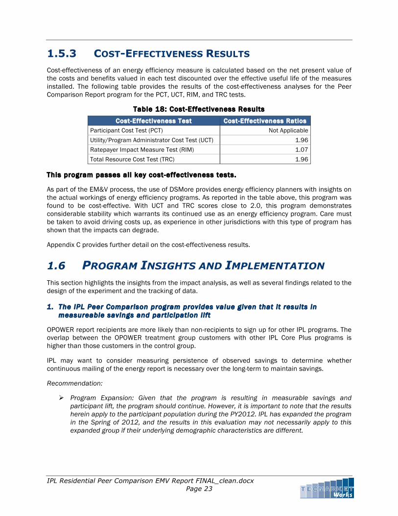
1.5.3 COST-EFFECTIVENESS RESULTS Cost-effectiveness of an energy efficiency measure is calculated based on the net present value of the costs and benefits valued in each test discounted over the effective useful life of the measures installed. The following table provides the results of the cost-effectiveness analyses for the Peer Comparison Report program for the PCT, UCT, RIM, and TRC tests.
Table 18: Cost-Effectiveness Results
Cost-Effectiveness Test Cost-Effectiveness Ratios Participant Cost Test (PCT) Not Applicable Utility/Program Administrator Cost Test (UCT) 1.96 Ratepayer Impact Measure Test (RIM) 1.07 Total Resource Cost Test (TRC) 1.96
This program passes al l key cost-effectiveness tests.
As part of the EM&V process, the use of DSMore provides energy efficiency planners with insights on the actual workings of energy efficiency programs. As reported in the table above, this program was found to be cost-effective. With UCT and TRC scores close to 2.0, this program demonstrates considerable stability which warrants its continued use as an energy efficiency program. Care must be taken to avoid driving costs up, as experience in other jurisdictions with this type of program has shown that the impacts can degrade.
Appendix C provides further detail on the cost-effectiveness results.
1.6 PROGRAM INSIGHTS AND IMPLEMENTATION This section highlights the insights from the impact analysis, as well as several findings related to the design of the experiment and the tracking of data.
1. The IPL Peer Comparison program provides value given that i t results in measureable savings and part ic ipation l i f t
OPOWER report recipients are more likely than non-recipients to sign up for other IPL programs. The overlap between the OPOWER treatment group customers with other IPL Core Plus programs is higher than those customers in the control group.
IPL may want to consider measuring persistence of observed savings to determine whether continuous mailing of the energy report is necessary over the long-term to maintain savings.
Recommendation:
Program Expansion: Given that the program is resulting in measurable savings and participant lift, the program should continue. However, it is important to note that the results herein apply to the participant population during the PY2012. IPL has expanded the program in the Spring of 2012, and the results in this evaluation may not necessarily apply to this expanded group if their underlying demographic characteristics are different.

IPL Residential Peer Comparison EMV Report FINAL_clean.docx Page 24
2. Lack of unique identif ier between the OPower dataset and the IPL customers create issues for program EM&V, specif ical ly the channeling analysis
OPOWER establishes its own unique identifier for the treatment and control group customers. While this creates an additional level of data security, it makes matching the OPOWER treatment and control population to other IPL CORE and Core Plus program tracking databases challenging. This requires a time consuming and less rigorous approach by match customer records based on name and address.
Recommendation:
The implementer should maintain the IPL unique customer identifier in its tracking database to enable channeling analysis. If this creates a security concern, then it should be a separate file that it can provide that provides the cross referenced unique IPL Account Identifiers against the unique OPOWER Account identifiers.

Appendix A: Fixed Effects Model (Email vs. Direct Mail)
IPL Residential Peer Comparison EMV Report FINAL_clean.docx Page 25
A. APPENDIX A: FIXED EFFECTS MODEL (DM VS. DM/EMAIL HOUSEHOLDS)
Below is a summary of the detailed model results. As described in the Analysis section, data are available both across households (i.e., cross-sectional) and over time (i.e., time-series). With this type of data, known as ‘panel’ data, it becomes possible to control, simultaneously, for differences across households as well as differences across periods in time through the use of a ‘fixed-effects’ panel model specification. The fixed-effect refers to the model specification aspect that differences across homes that do not vary over the estimation period (such as square footage, heating system, etc.) can be explained, in large part, by customer-specific intercept terms that capture the net change in consumption due to the program, controlling for other factors that do change with time (e.g., the weather). Moreover, for a comparison report program like this, a treatment vs. control group approach is commonly used. A proc glm procedure in SAS was utilized to construct the FE model.
This model can be expressed as:
Equation 7: Fixed Effect Model – DM/email vs. DM Savings
𝑘𝑊ℎ!" = 𝛼! + 𝛼!𝑀𝑜𝑛𝑡ℎ𝐼𝐷! + 𝛼!𝐶𝐷𝐷!" + 𝛼!𝐻𝐷𝐷!" + 𝛽!𝑃𝑜𝑠𝑡!𝐸𝑚𝑎𝑖𝑙! + 𝛽!𝑃𝑜𝑠𝑡!𝐷𝑀!+ 𝛽!𝑃𝑜𝑠𝑡!𝑃𝑎𝑟𝑡!𝐸𝑚𝑎𝑖𝑙! + 𝛽!𝑃𝑜𝑠𝑡!𝑃𝑎𝑟𝑡!𝐸𝑚𝑎𝑖𝑙! + 𝜀!"
Specifically this model includes six variables:
1. 𝛼! − Utility_customer_ID: this is where the fixed effect comes. It serves as a by-account intercept which captures the differences across homes that do not vary over the estimation period (such as square footage, heating system, etc.)
2. MonthID: it is a dummy variable which equals to 1 for the corresponding month and 0 otherwise. This variable is used to control for the macroeconomic conditions.
3. CDD: cooling degree days which capture the weather effect
4. HDD: heating degree days which capture the weather effect
5. Post * DM: It is a multiplication of the variable ‘Post’ and the variable ‘DM’. Post9 is a dummy variable which equals to one if the month is in the post-program period; 0 otherwise. DM is a categorical variable which equals to one where DM is available for both treatment and control group members, 0 otherwise. ‘Post*DM ‘measures during the post-program period how the direct mail recipient changed their consumption (given email = 0);
6. Post*email: It is a multiplication of the variable ‘Post’ and the variable ‘Email’. Email is a categorical variable which equals to one where email is available for both treatment and control group members, 0 otherwise. ‘Post*email” measures during the post-program period how the email recipient changed their consumption (given email = 1). Note these
9 The very first month during which the first report was sent was deleted from the analysis. For example if the first report went out on March 9th within a billing period of March 1st – March 31st, March is considered “dead-band” and is excluded from the analysis. This is a consistent approach across the other Indiana utilities.

Appendix A: Fixed Effects Model (Email vs. Direct Mail)
IPL Residential Peer Comparison EMV Report FINAL_clean.docx Page 26
consumption changes are NOT caused by the report because it is estimated based on treatment and control group members;
7. Post*Part*DM: it is a multiplication of the variable ‘Post’, ‘Part’ and the variable ‘DM’. Post as previously discussed tracks the post-program period. ‘Part’ is a dummy that tracks treatment group membership: i.e. Part equals to one if a customer is included in the treatment group, 0 otherwise. ‘Post*Part*DM’ measures during the post-program period how the report had changed the consumption of direct mail recipients;
8. Post*Part*email: it is a multiplication of the variable ‘Post’, ‘Part’ and the variable ‘Email’. Post as previously discussed tracks the post-program period. ‘Part’ is a dummy that tracks treatment group membership: i.e. Part equals to one if a customer is included in the treatment group, 0 otherwise. Post*Part tracks the treatment group membership during the post-program period; ‘Post*Part*email’ measures during the post-program period how program treatment (report and email) changed the consumption of email recipients.
Number of Observations Read 1657335
Dependent Variable: kwh Sum of Source DF Squares Mean Square F Value Pr > F Model 43361 870497731207 20075591.689 40.79 <.0001 Error 1.61E6 794346690544 492168.51245 Corrected Total 1.66E6 1.6648444E12 R-‐Square Coeff Var Root MSE kwh Mean 0.522870 33.08988 701.5472 2120.126 Source DF Type I SS Mean Square F Value Pr > F utility_customer_id 43303 304727776820 7037105.4389 14.30 <.0001 monthID 52 517451267748 9950985918.2 20218.7 <.0001 cdd 1 6266461895 6266461895 12732.4 <.0001 hdd 1 41914369556 41914369556 85162.6 <.0001 post*email 2 97241830.332 48620915.166 98.79 <.0001 post*part*email 2 40613356.218 20306678.109 41.26 <.0001 Source DF Type III SS Mean Square F Value Pr > F monthID 52 24360993744 468480649 951.87 <.0001 cdd 1 7568704795 7568704795 15378.3 <.0001 hdd 1 41878715293 41878715293 85090.2 <.0001 post*email 2 29071757 14535878 29.53 <.0001 post*part*email 2 40613356 20306678 41.26 <.0001
Appendix A: Fixed Effects Model (Email vs. Direct Mail)
IPL Residential Peer Comparison EMV Report FINAL_clean.docx Page 27
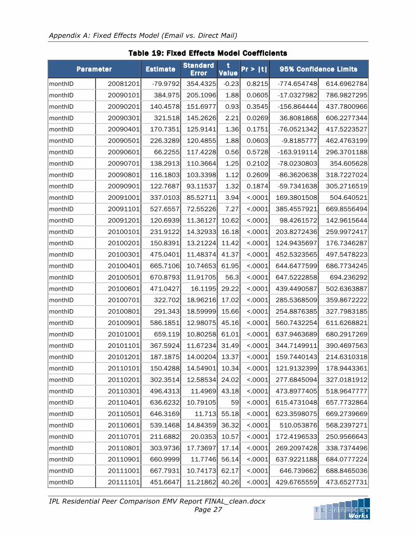
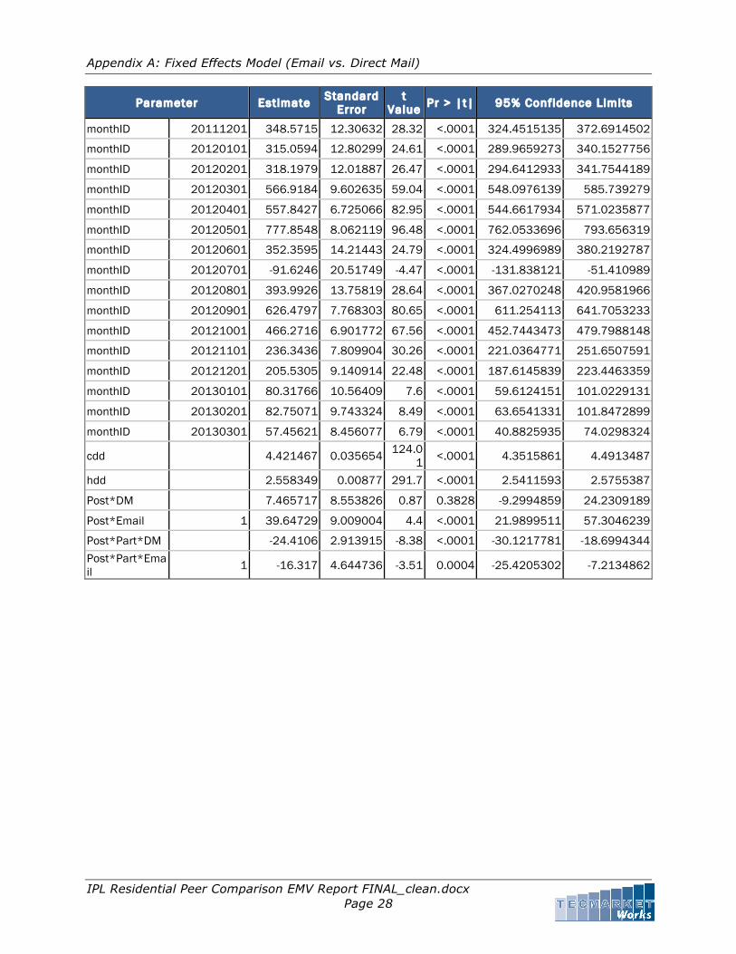
Table 19: Fixed Effects Model Coeff ic ients
Parameter Estimate Standard Error
t Value Pr > |t| 95% Confidence Limits
monthID 20081201 -79.9792 354.4325 -0.23 0.8215 -774.654748 614.6962784
monthID 20090101 384.975 205.1096 1.88 0.0605 -17.0327982 786.9827295
monthID 20090201 140.4578 151.6977 0.93 0.3545 -156.864444 437.7800966
monthID 20090301 321.518 145.2626 2.21 0.0269 36.8081868 606.2277344
monthID 20090401 170.7351 125.9141 1.36 0.1751 -76.0521342 417.5223527
monthID 20090501 226.3289 120.4855 1.88 0.0603 -9.8185777 462.4763199
monthID 20090601 66.2255 117.4228 0.56 0.5728 -163.919114 296.3701188
monthID 20090701 138.2913 110.3664 1.25 0.2102 -78.0230803 354.605628
monthID 20090801 116.1803 103.3398 1.12 0.2609 -86.3620638 318.7227024
monthID 20090901 122.7687 93.11537 1.32 0.1874 -59.7341638 305.2716519
monthID 20091001 337.0103 85.52711 3.94 <.0001 169.3801508 504.640521
monthID 20091101 527.6557 72.55226 7.27 <.0001 385.4557921 669.8556494
monthID 20091201 120.6939 11.36127 10.62 <.0001 98.4261572 142.9615644
monthID 20100101 231.9122 14.32933 16.18 <.0001 203.8272436 259.9972417
monthID 20100201 150.8391 13.21224 11.42 <.0001 124.9435697 176.7346287
monthID 20100301 475.0401 11.48374 41.37 <.0001 452.5323565 497.5478223
monthID 20100401 665.7106 10.74653 61.95 <.0001 644.6477599 686.7734245
monthID 20100501 670.8793 11.91705 56.3 <.0001 647.5222858 694.236292
monthID 20100601 471.0427 16.1195 29.22 <.0001 439.4490587 502.6363887
monthID 20100701 322.702 18.96216 17.02 <.0001 285.5368509 359.8672222
monthID 20100801 291.343 18.59999 15.66 <.0001 254.8876385 327.7983185
monthID 20100901 586.1851 12.98075 45.16 <.0001 560.7432254 611.6268821
monthID 20101001 659.119 10.80258 61.01 <.0001 637.9463689 680.2917269
monthID 20101101 367.5924 11.67234 31.49 <.0001 344.7149911 390.4697563
monthID 20101201 187.1875 14.00204 13.37 <.0001 159.7440143 214.6310318
monthID 20110101 150.4288 14.54901 10.34 <.0001 121.9132399 178.9443361
monthID 20110201 302.3514 12.58534 24.02 <.0001 277.6845094 327.0181912
monthID 20110301 496.4313 11.4969 43.18 <.0001 473.8977405 518.9647777
monthID 20110401 636.6232 10.79105 59 <.0001 615.4731048 657.7732864
monthID 20110501 646.3169 11.713 55.18 <.0001 623.3598075 669.2739669
monthID 20110601 539.1468 14.84359 36.32 <.0001 510.053876 568.2397271
monthID 20110701 211.6882 20.0353 10.57 <.0001 172.4196533 250.9566643
monthID 20110801 303.9736 17.73697 17.14 <.0001 269.2097428 338.7374496
monthID 20110901 660.9999 11.7746 56.14 <.0001 637.9221188 684.0777224
monthID 20111001 667.7931 10.74173 62.17 <.0001 646.739662 688.8465036
monthID 20111101 451.6647 11.21862 40.26 <.0001 429.6765559 473.6527731
Appendix A: Fixed Effects Model (Email vs. Direct Mail)
IPL Residential Peer Comparison EMV Report FINAL_clean.docx Page 28
Parameter Estimate Standard Error
t Value Pr > |t| 95% Confidence Limits
monthID 20111201 348.5715 12.30632 28.32 <.0001 324.4515135 372.6914502
monthID 20120101 315.0594 12.80299 24.61 <.0001 289.9659273 340.1527756
monthID 20120201 318.1979 12.01887 26.47 <.0001 294.6412933 341.7544189
monthID 20120301 566.9184 9.602635 59.04 <.0001 548.0976139 585.739279
monthID 20120401 557.8427 6.725066 82.95 <.0001 544.6617934 571.0235877
monthID 20120501 777.8548 8.062119 96.48 <.0001 762.0533696 793.656319
monthID 20120601 352.3595 14.21443 24.79 <.0001 324.4996989 380.2192787
monthID 20120701 -91.6246 20.51749 -4.47 <.0001 -131.838121 -51.410989
monthID 20120801 393.9926 13.75819 28.64 <.0001 367.0270248 420.9581966
monthID 20120901 626.4797 7.768303 80.65 <.0001 611.254113 641.7053233
monthID 20121001 466.2716 6.901772 67.56 <.0001 452.7443473 479.7988148
monthID 20121101 236.3436 7.809904 30.26 <.0001 221.0364771 251.6507591
monthID 20121201 205.5305 9.140914 22.48 <.0001 187.6145839 223.4463359
monthID 20130101 80.31766 10.56409 7.6 <.0001 59.6124151 101.0229131
monthID 20130201 82.75071 9.743324 8.49 <.0001 63.6541331 101.8472899
monthID 20130301 57.45621 8.456077 6.79 <.0001 40.8825935 74.0298324
cdd 4.421467 0.035654 124.01 <.0001 4.3515861 4.4913487
hdd 2.558349 0.00877 291.7 <.0001 2.5411593 2.5755387
Post*DM 7.465717 8.553826 0.87 0.3828 -9.2994859 24.2309189
Post*Email 1 39.64729 9.009004 4.4 <.0001 21.9899511 57.3046239
Post*Part*DM -24.4106 2.913915 -8.38 <.0001 -30.1217781 -18.6994344 Post*Part*Email 1 -16.317 4.644736 -3.51 0.0004 -25.4205302 -7.2134862

Appendix B: Fixed Effects Model Output for Overall Program
IPL Residential Peer Comparison EMV Report FINAL_clean.docx Page 29
B. APPENDIX B: FIXED EFFECTS MODEL OUTPUT FOR OVERALL PROGRAM
Below is a summary of the detailed model results. As described in the Analysis section, data are available both across households (i.e., cross-sectional) and over time (i.e., time-series). With this type of data, known as ‘panel’ data, it becomes possible to control, simultaneously, for differences across households as well as differences across periods in time through the use of a ‘fixed-effects’ panel model specification. The fixed-effect refers to the model specification aspect that differences across homes that do not vary over the estimation period (such as square footage, heating system, etc.) can be explained, in large part, by customer-specific intercept terms that capture the net change in consumption due to the program, controlling for other factors that do change with time (e.g., the weather). Moreover for a comparison report program like this, a treatment – control group approach is commonly used. The model specification is:
Equation 8: Fixed Effect Model – Direct Overal l Savings
𝑘𝑊ℎ!" = 𝛼! + 𝛼!𝑀𝑜𝑛𝑡ℎ𝐼𝐷! + 𝛼!𝐶𝐷𝐷!" + 𝛼!𝐻𝐷𝐷!" + 𝛽!𝑃𝑜𝑠𝑡! + 𝛽!𝑃𝑜𝑠𝑡!𝑃𝑎𝑟𝑡! + 𝜀!"
Specifically this model includes five variables:
1. 𝛼!: The utility customer ID, where the fixed effect comes from (denoted by Utility_customer_ID in the model output below) It serves as a by-account intercept which captures the differences across homes that do not vary over the estimation period (such as square footage, heating system, etc.)
2. MonthIDt: it is a dummy variable which equals to 1 for the corresponding month and 0 otherwise. This variable is used to control for the macro economic conditions.
3. CDDi: cooling degree days which capture the weather effect
4. HDDi: heating degree days which capture the weather effect
5. Postt: Post is a dummy variable which equals to one if the month is in the post-program period; 0 otherwise.
6. 𝑃𝑜𝑠𝑡!𝑃𝑎𝑟𝑡!: It is an interaction of the variable ‘Post’ and the variable ‘Participation’. Participation is also a dummy variable which equals to one if a customer received reports, 0 otherwise.
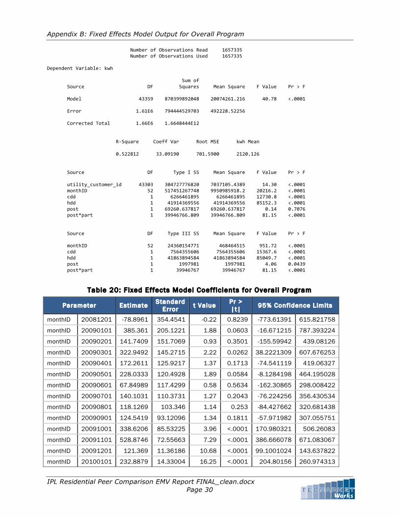
Appendix B: Fixed Effects Model Output for Overall Program
IPL Residential Peer Comparison EMV Report FINAL_clean.docx Page 30
Number of Observations Read 1657335 Number of Observations Used 1657335 Dependent Variable: kwh Sum of Source DF Squares Mean Square F Value Pr > F Model 43359 870399892048 20074261.216 40.78 <.0001 Error 1.61E6 794444529703 492228.52256 Corrected Total 1.66E6 1.6648444E12 R-‐Square Coeff Var Root MSE kwh Mean 0.522812 33.09190 701.5900 2120.126 Source DF Type I SS Mean Square F Value Pr > F utility_customer_id 43303 304727776820 7037105.4389 14.30 <.0001 monthID 52 517451267748 9950985918.2 20216.2 <.0001 cdd 1 6266461895 6266461895 12730.8 <.0001 hdd 1 41914369556 41914369556 85152.3 <.0001 post 1 69260.637817 69260.637817 0.14 0.7076 post*part 1 39946766.809 39946766.809 81.15 <.0001 Source DF Type III SS Mean Square F Value Pr > F monthID 52 24360154771 468464515 951.72 <.0001 cdd 1 7564355606 7564355606 15367.6 <.0001 hdd 1 41863894584 41863894584 85049.7 <.0001 post 1 1997981 1997981 4.06 0.0439 post*part 1 39946767 39946767 81.15 <.0001
Table 20: Fixed Effects Model Coeff ic ients for Overal l Program
Parameter Estimate Standard Error t Value Pr >
|t| 95% Confidence Limits
monthID 20081201 -78.8961 354.4541 -0.22 0.8239 -773.61391 615.821758
monthID 20090101 385.361 205.1221 1.88 0.0603 -16.671215 787.393224
monthID 20090201 141.7409 151.7069 0.93 0.3501 -155.59942 439.08126
monthID 20090301 322.9492 145.2715 2.22 0.0262 38.2221309 607.676253
monthID 20090401 172.2611 125.9217 1.37 0.1713 -74.541119 419.06327
monthID 20090501 228.0333 120.4928 1.89 0.0584 -8.1284198 464.195028
monthID 20090601 67.84989 117.4299 0.58 0.5634 -162.30865 298.008422
monthID 20090701 140.1031 110.3731 1.27 0.2043 -76.224256 356.430534
monthID 20090801 118.1269 103.346 1.14 0.253 -84.427662 320.681438
monthID 20090901 124.5419 93.12096 1.34 0.1811 -57.971982 307.055751
monthID 20091001 338.6206 85.53225 3.96 <.0001 170.980321 506.26083
monthID 20091101 528.8746 72.55663 7.29 <.0001 386.666078 671.083067
monthID 20091201 121.369 11.36186 10.68 <.0001 99.1001024 143.637822
monthID 20100101 232.8879 14.33004 16.25 <.0001 204.80156 260.974313

Appendix B: Fixed Effects Model Output for Overall Program
IPL Residential Peer Comparison EMV Report FINAL_clean.docx Page 31
Parameter Estimate Standard Error t Value Pr >
|t| 95% Confidence Limits
monthID 20100201 151.7179 13.21289 11.48 <.0001 125.821075 177.614703
monthID 20100301 475.7397 11.48433 41.43 <.0001 453.230822 498.248604
monthID 20100401 666.2569 10.74712 61.99 <.0001 645.192883 687.320839
monthID 20100501 671.5152 11.91769 56.35 <.0001 648.156903 694.873419
monthID 20100601 471.8736 16.12038 29.27 <.0001 440.278177 503.468934
monthID 20100701 323.6559 18.9632 17.07 <.0001 286.488722 360.823149
monthID 20100801 292.2853 18.601 15.71 <.0001 255.827939 328.742591
monthID 20100901 586.8672 12.98145 45.21 <.0001 561.424001 612.310404
monthID 20101001 659.6876 10.80316 61.06 <.0001 638.513744 680.861385
monthID 20101101 368.3105 11.67294 31.55 <.0001 345.431921 391.189033
monthID 20101201 188.1287 14.00273 13.44 <.0001 160.683809 215.573536
monthID 20110101 151.4113 14.54972 10.41 <.0001 122.894349 179.928253
monthID 20110201 303.1601 12.58598 24.09 <.0001 278.492006 327.828173
monthID 20110301 497.1155 11.49749 43.24 <.0001 474.580789 519.650166
monthID 20110401 637.1869 10.79164 59.04 <.0001 616.035643 658.33811
monthID 20110501 646.9475 11.71363 55.23 <.0001 623.989217 669.905839
monthID 20110601 539.9 14.8444 36.37 <.0001 510.805506 568.994526
monthID 20110701 212.6742 20.0364 10.61 <.0001 173.403539 251.944858
monthID 20110801 304.8661 17.73794 17.19 <.0001 270.100333 339.631834
monthID 20110901 661.6113 11.77523 56.19 <.0001 638.532213 684.690316
monthID 20111001 668.3417 10.74231 62.22 <.0001 647.287185 689.396314
monthID 20111101 452.2971 11.21921 40.31 <.0001 430.30782 474.286362
monthID 20111201 349.3413 12.30695 28.39 <.0001 325.220116 373.462512
monthID 20120101 315.8804 12.80364 24.67 <.0001 290.785729 340.975109
monthID 20120201 318.9412 12.01948 26.54 <.0001 295.383392 342.49893
monthID 20120301 567.5647 9.60311 59.1 <.0001 548.742952 586.38648
monthID 20120401 558.0172 6.72546 82.97 <.0001 544.835502 571.198842
monthID 20120501 778.0474 8.062595 96.5 <.0001 762.245005 793.849822
monthID 20120601 352.789 14.21526 24.82 <.0001 324.927553 380.650395
monthID 20120701 -90.9846 20.51869 -4.43 <.0001 -131.2005 -50.768663
monthID 20120801 394.3497 13.75901 28.66 <.0001 367.382568 421.31693
monthID 20120901 626.5986 7.768769 80.66 <.0001 611.37213 641.825168
monthID 20121001 466.368 6.902185 67.57 <.0001 452.839906 479.895995
monthID 20121101 236.5437 7.810363 30.29 <.0001 221.23568 251.851762
monthID 20121201 205.8359 9.141441 22.52 <.0001 187.918982 223.752797
monthID 20130101 80.70798 10.56469 7.64 <.0001 60.0015487 101.414407
monthID 20130201 83.06798 9.743887 8.53 <.0001 63.9702937 102.165658

Appendix B: Fixed Effects Model Output for Overall Program
IPL Residential Peer Comparison EMV Report FINAL_clean.docx Page 32
Parameter Estimate Standard Error t Value Pr >
|t| 95% Confidence Limits
monthID 20130301 57.66288 8.456576 6.82 <.0001 41.0882828 74.2374762
cdd 4.420182 0.035656 123.97 <.0001 4.350297 4.4900677
hdd 2.557877 0.008771 291.63 <.0001 2.5406863 2.5750676
post 17.05127 8.463394 2.01 0.0439 0.4633127 33.6392307
post*part -22.2379 2.46852 -9.01 <.0001 -27.076133 -17.399704

IPL Residential Peer Comparison EMV Report FINAL_clean.docx Page 33
C. APPENDIX C: COST EFFECTIVENESS DETAIL TABLES
Note: For the Participant Test, when there are no participant costs, DSMore returns a value of 65535.

Summary of Findings
IPL Residential Peer Comparison EMV Report FINAL_clean.docx Page 34