2008:079

M A S T E R ' S T H E S I S

Reflector Simulation programfor an imaging air Cherenkov

telescope

Zhe Qi

Luleå University of Technology

Master Thesis, Continuation Courses Space Science and Technology

Department of Space Science, Kiruna

2008:079 - ISSN: 1653-0187 - ISRN: LTU-PB-EX--08/079--SE

Reflector Simulation program for an ImagingAir Cherenkov Telescope

Master Thesisby

Qi,Zhe

Erasmus Mundus SpaceMaster

AtBayerische Julius-Maximilians-Universität Würzburg, Germany

Luleå University of Technology, Sweden

September, 2007

1

Abstract

In the last 20 years the ground-based telescopes have opened a new observation window at very highenergies(VHE) between 100 GeV and 10 TeV, with the application of imaging air Cherenkovtechnique. Here the Cherenkov light from secondary particles produced in electromagnetic cascades,initiated from a primary γ-photon or a charged particle, is measured. As these Cherenkov light flashesare very faint and short, a large reflector as well as a high sensitivity photo-multiplier camera is used.From the images of the air shower, the identity and energy of the primary particle could bereconstructed. The base for this reconstruction is the comparison with artificial air showers producedby Monte Carlo simulations and processed through a complete detector simulation. The currentgeneration of large Imaging Air Cherenkov telescopes, as MAGIC or H.E.S.S is not practical for longtime monitoring of certain sources, mainly for cost reasons. Therefore a new instrument is proposed,which is dedicated to long time observations of bright nearby blazars. It is based on a technical upgradeof one of the former Cherenkov telescopes of the HEGRA experiment. The observation targets areextragalactic objects, that show non-thermal broad band emission from the radio band up to VHEgamma-rays. Among the most extreme astrophysical objects, blazers emit most of their energy at γ-rays and show time variability in scales from years down to several minutes. So far, long termmonitoring lack from the small sampling of the light curve at VHE. For the ongoing studies of theinstrument and coming data analysis, a new detector simulation is necessary. In this work, the reflectionof Cherenkov photons, produced with the air shower simulation program CORSIKA [Heck etal.(1998)], at a user-defined reflector with user-defined properties is simulated and introduced in theexisting framework MARS. The detector simulations presented in the end show comparable results tothe MAGIC reflector.

2

Table of Contents

Chapter 1: Introduction .............................................................................................................................41.1 Project Overview.............................................................................................................................41.2 Task Statement ................................................................................................................................51.3 Layout of the paper..........................................................................................................................6

Chapter 2: Background .............................................................................................................................72.1 Brief review of VHE Gamma-ray Astronomy.................................................................................7

2.1.1 Introduction............................................................................................................................7 2.1.2 Detecting Technique...............................................................................................................9

2.2 Cherenkov Radiation.....................................................................................................................102.3 Hadronic and Gamma-ray Air Shower..........................................................................................132.4 Detecting Air Showers with Imaging Air Cherenkov Telescope...................................................15

Chapter 3: Reading CORSIKA File .......................................................................................................183.1 Monte Carlo Simulation................................................................................................................183.2 Analysis Tools...............................................................................................................................183.3 CORSIKA 6.500...........................................................................................................................18

3.3.1 Introduction .........................................................................................................................18 3.3.2 Program model options.........................................................................................................19 3.3.3 Data Files..............................................................................................................................20

3.4 Algorithm.......................................................................................................................................243.5 Results..........................................................................................................................................25

Chapter 4: Reflector Simulation .............................................................................................................284.1 Introduction...................................................................................................................................284.2 MAGIC Reflector..........................................................................................................................294.3 Algorithm ......................................................................................................................................304.4 Results and Discussion..................................................................................................................34

Chapter 5: Conclusion and Future work .................................................................................................44Reference List 46

Appendix: Data Structure of CORSIKA 48

3

Chapter 1: Introduction

1.1 Project OverviewMAGIC (Major Atmosphere Gamma-ray Imaging Cherenkov telescope) is an Imaging AtmosphericCherenkov telescope designed to observe Very High Energy(VHE) gamma rays from astrophysicalsources. It is located on the Canary Islands of La Palma (28º N and 17º W), Spain at about 2200 metersabove sea level.

As a new generation of imaging atmospheric Cherenkov telescope, the first design proposal of MAGICis presented in 1995 (Brad et al.,1995) with the lowest possible threshold energy. Based on theexperience acquired with the first generation of Cherenkov telescope, the whole construction ofMAGIC has been completed in 2003 supported primarily by the funding agencies BMBF (Germany),MPG (Germany), INFN (Italy), CICYT (Spain) and SNF (Switzerland). Since 2004, it has beenoperated under the MAGIC collaboration of 17 institutes [1] around the world.

MAGIC telescope collects very short flashes of atmospheric Cherenkov radiation (< 10 nsec induration) emitted during the development of the air showers produced in the interaction of the gammarays with the atmospheric nuclei. As the world largest single dish reflector, MAGIC telescope (seeFigure 1 ) has

➢ A 17 m diameter parabolic mirror with f / D= 1.

➢ A reflecting surface of 236 m² consisting of 50 cm × 50 cm reflectors.

➢ A camera as a hexagonal array of 577 fast-response photomultiplier tubes (PMTs) which has aquantum efficiency (QE) around 30%.

4

Figure 1: The 17 m diameter MAGIC telescope on the Canary Island ofLa Palma. Taken by R.Wagner.

➢ An active mirror control (AMC) system that is able to correct the mirror pointing on-line fordish deformations.

➢ A multilevel trigger and a 300 MHz FADC system for pulse digitalization (replaced by a 2GHzdigital system in February 2007).

➢ Signal transmission by using analog optical fiber signal.

The research target of MAGIC telescope include [2]:

➢ The study of Active Galactic Nuclei (AGN).

➢ Observation of Gamma Ray Bursts (GRBs) in the new energy window.

➢ The study of galactic gamma sources such as supernova remnants, pulsars and binary systems.

Since its commissioning in 2004, numerous new sources have been detected at VHE level. Currently asecond telescope is under construction on the same site for stereoscopic observations with the aim oflowering the energy threshold and increasing the sensitivity. Its foundation, frame and drive equipmentsare already in place and it is expected to start commissioning in 2008.

1.2 Task Statement For the construction of future IACT detectors, two main issues in principle have to be considered: theastrophysical significance (observing targets); and the experimental feasibility (cost).

The discovery of new, faint objects has become the major task for the new generation telescopes.Blazars are highly compact and variable sources associated with supermassive blackholes at the centerof a galaxy. Blazars are believed to be a subclass of Active Galactic Nuclei (AGN) (shown in Figure 2)[4] and can be divided into two groups: highly variable quasars and BL Lacertae objects. Among allAGNs, blazars emit over the widest range of frequencies being detected from radio to gamma-ray.

Long term observations of bright blazars are the key to obtain a solid database for variabilityinvestigation. However observations with telescopes like MAGIC are very expensive and impracticalfor long term run, only possible with a dedicated instrument. A small imaging air Cherenkov telescopeis currently being built. It is based on the upgrade of the former CT3 of the High Energy Gamma-RayArray (HERGA) with low-cost but high sensitivity. Assuming the performance of the new telescopecomparable to the HEGRA – telescope, it is suited for long term monitoring of the following targets[3]:

➢ Mrk421

➢ Mrk501

➢ 1ES 2344+514

➢ 1ES 1959+650

➢ H 1426+428

➢ PKS 2155-304

5

More details regarding the technical set up of the dedicated telescope can be found in [3].

For future studies of the instruments and analysis of the data, a new detector simulation is necessary. Anew modular method will be implemented into the existing software framework “MARS” (MagicAnalysis and Reconstruction Software). In this work, the reflection of Cherenkov photons simulatedwith CORSIKA at a user-defined reflector with user-defined properties is implemented into the existinganalysis tool. The programming language is C++. The reflection code is based on the CERN's analysispackage ROOT and fit into MARS framework.

1.3 Layout of the paperIn the following chapter, a brief review regarding very high energy gamma ray astronomy is reviewed.Chapter 3 suggests the algorithm in MARS of reading CORSIKA file. Simulations of the reflector andanalysis of the results are presented and discussed in chapter 4. The final chapter holds the conclusionand future work suggestion.

6

Figure 2: Blazars are AGNs which has one of its relativisticjets pointed toward the Earth so the emission being observedis dominated by phenomena occurring in the jet regionaccounting for the variability and compact features of bothtypes of blazars. Central black hole capture the gas, dust andstars creating a accretion disk which generates huge amountsof energy in the form of elementary particles. Also a largeopaque torus extending from the center black hole. The cloudwill absorb and emit from regions closer to the black hole andit can be detected on Earth as emission lines in the blazarspectrum. A pair of relativistic jets, which is perpendicular tothe accretion disk, carry a high energy plasma away from theAGN. The “direction”of jet is depending on the combinationof magnetic fields and winds from the accretion disk andtorus. Referred to [4].

Chapter 2: Background

2.1 Brief review of VHE Gamma-ray Astronomy

2.1.1 Introduction

Cosmic Rays were discovered by Austrian scientist Victor Hess (Nobel Prize, 1936) in the beginning of20th century through a balloon experiment of the ionizing effect on airtight vessels of glass enclosingtwo electrodes with a high voltage between them. The ionizing effect increased as the balloon climbedup and therefore it demonstrated that the radiation must come from the outer space. So the term CosmicRays was dubbed. Since then, various of experiments and observations have been carried outworldwide and this new field of astrophysics has been rapidly developing.

Cosmic rays are energetic charged particles that possess a large range of energies from 106 electron-volt(eV) to more than 1020 eV. Cosmic rays mainly consist of high energy nuclear particles (protons as wellas heavier atomic nuclei), a small fraction of electrons and an even smaller fraction of photons in theform of gamma-rays (< 10-4) which are important for astronomers when trying to find out the origin ofcosmic rays.

Until now, the origin of cosmic rays is still not well understood. The charged components of cosmicrays are deflected by the galactic or intergalactic magnetic fields and hit the Earth from all directions.Therefore, the charged component can not be used to trace the particles back to their origin, onlypossible with the neutral components such as gamma rays, which have no electrical charge and arriveat the Earth undeflected. With the direction information, gamma ray particles make the search andinvestigation of cosmic ray sources possible.

7

Figure 3: Left: In the form of a flashlight beam, a jet of electrons and protons traveling near thespeed of light seen in Hubble's image. The beam is gushing outward from the center of thegalaxy M87 that lies around 50 million light-years away from Earth. Referred to [5].

Right: Crab Nebula, as the remnant of a star began its life with about 10 times the mass of Sun.Referred to [6].

Very High Energy (VHE) gamma-ray astronomy is the study of photons in the 10 GeV to 100 TeVenergy range (see Table 1).

Table 1: Classification of the energy regions in gamma-ray astronomy. Taken from [7].

Energy Range Classification Detecting Technique 0.1 – 10 MeV Low Energy (LE) Space-based 10 - 30 MeV Medium Energy (ME) Space-based 30 MeV – 10 GeV High Energy (HE) Space-based 10 GeV – 100 TeV Very High Energy (VHE) Ground-based 100 TeV – 100 PeV Ultra High Energy (UHE) Ground-based 100 PeV – 100 EeV Extremely High Energy (EHE) Ground-based

The photons are produced by the exotic objects in the universe among the detected source categories.Following are several types of astrophysical objects that could emit gamma-rays:

➢ Active Galactic Nuclei (AGN): A supermassive black hole at the center of a galaxy attractsmatter by gravitational force.

➢ Supernova Remnant (SNR): the remains of a supernova explosion bounded by an expandingshock wave.

➢ Pulsars: a rotating neutron starts that generates regular pulses of radiation at its spin rate.

➢ Gamma-ray bursts (GRB): intense flashes that radiate tremendous amounts of energy in theform of gamma rays.

➢ Binary systems: Cataclysmic variables (CV), X-ray Binaries (XRB) and microquasars.

High-energy gamma radiation are produced via the following main processes as:

➢ Inverse Compton scattering: Interaction of high energy (relativistic) electron with low energyphoton. The net energy is transferred from electron to the photon.

➢ Pion decay: The neutral meson decays due to electromagnetic force. π0 decays into two gammarays with a probability of 99%.

➢ Bremsstrahlung: Electromagnetic radiation produced by a sudden slowing down of chargedparticles passing through matter in the vicinity of electric fields of atomic nuclei.

➢ Synchrotron radiation: A special case of inverse Compton scattering. Radiation occurs whencharged particles are following a curved trajectory - for example the charged particles under theinfluence of a magnetic field.

The study of VHE γ-ray may help to determine the source of cosmic rays, allow us to understand howmatter and radiation interact with each other under extreme conditions. It provides a completelydifferent view of the universe from other types of radiation. VHE γ-ray astronomy reveals theextraordinary relativistic objects which offer a sensitive study of fundamental physics and astrophysicalprocesses.

8

2.1.2 Detecting Technique

Gamma rays are detected and measured with balloon flights, satellites and ground arrays. Theinstruments-chosen depend strongly on the energy range of the primary particles.

Space-based detectors

The detecting technique of a given energy range of gamma-rays is depending on its arrival rate whichvaries enormously with their energy. The drop rate of LE and ME gamma-rays flux is many thousandsper square meter every second that makes the direct measurement possible.

The atmosphere absorbs most of the gamma-rays before they reach the ground. To measure the primarygamma-rays directly without atmospheric disturbances, the detection equipment should be placedabove the atmosphere, which can be accomplished by carrying the instruments aboard the high-altitudeballoons or Earth-orbit satellites. The first gamma-ray telescope sensitive to energies greater than 50MeV was carried into orbit on the satellite “Explore XI “ in 1961. Since then, more detectors were sentinto orbit providing spectacular discovery. However, the poor resolution of the instruments limit thefurther development. After the launch of the Compton Gamma-Ray Observation (CGRO), the situationhas been improved. Planned and built by NASA, CGRO went into orbit in April 1991 and continued tooperate until June, 2000. The telescope EGRET (Energetic Gamma Ray Experiment Telescope), one ofthe four payloads on board, covers the energy range from 30 KeV to 30GeV. It greatly improved thespatial and temporal resolution and provided the best look of gamma-rays ever since, which improvesthe understanding of high energy processes in the universe. The third EGRET Catalog consists of 271sources (E >100 MeV): 5 pulsars, 1 solar flare, 66 high-confidence blazar identifications, 27 possibleblazar identifications, 1 likely radio galaxy (Cen A), 1 normal galaxy (LMC) and 170 unidentifiedsources as shown in Figure 4.

As one of the next generation gamma-ray observatory, GLAST (Gamma-ray Large Area SpaceTelescope) is designed to probe for gamma-ray bursts, black hole particle jets and other celestial

9

Figure 4: The third EGRET catalog. Referred to [8].

sources in the energy band extending from 10 KeV to more than 300 GeV, the broadest energycoverage ever provided by a single spacecraft for gamma-ray studies. It is scheduled to launch inJanuary, 2008 by the cooperation of NASA with United States Department of Energy. During the lastyears numerous sources in GeV range have been localized with the aid of space-based detectors.

Ground-based detectors

Above the VHE region, the gamma-rays are rare and the flux drops to below one particle per squaremeter per year, which makes direct measurements impractical. The only possible solution is to observethe γ-ray induced air showers by ground-based telescopes with the application of the ImagingAtmosphere Cherenkov Technique (IACT). In this case, the Earth's atmosphere is served as thedetection medium, implying a collection area of many hundreds of square meters. The IACT, proposedby Weekes and Turver in 1977, works by imaging the very brief flash of Cherenkov radiation generatedby the cascade of charged particles produced when a VHE gamma-ray hits the atmosphere. The showerof charged particles, known as an Air Shower, is initiated at a height of about 20 km. The total area onthe ground illuminated by the flash is usually corresponding to many hundreds of square meters – themajority of secondary particles is within ~ 200 m distance to the shower axis.

The Whipple 10m telescope is the first IACT telescope to be operated. The first VHE γ-ray source itdetected was presented in 1989 when gamma-ray emission from Crab Nebula (shown in Figure 3) wasobserved. Since then, several other IACT telescopes have been built and the catalog of detected γ-raysources has been increased to nearly 20 objects (Horan and Weekes, 2004).

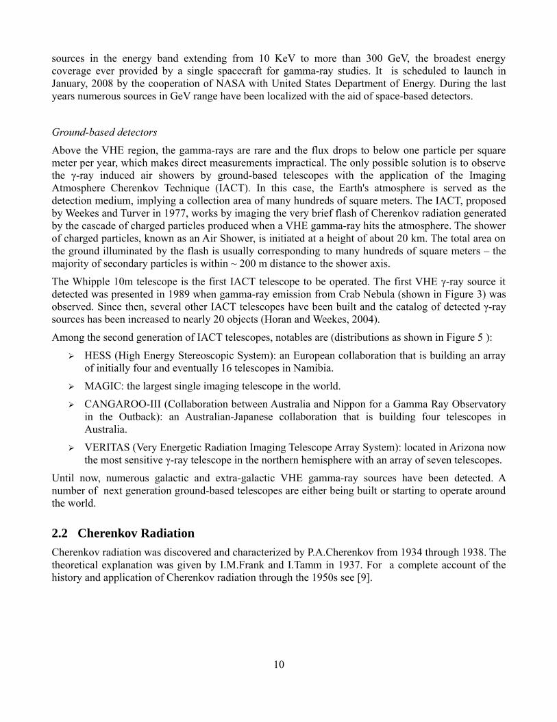
Among the second generation of IACT telescopes, notables are (distributions as shown in Figure 5 ):

➢ HESS (High Energy Stereoscopic System): an European collaboration that is building an arrayof initially four and eventually 16 telescopes in Namibia.

➢ MAGIC: the largest single imaging telescope in the world.

➢ CANGAROO-III (Collaboration between Australia and Nippon for a Gamma Ray Observatoryin the Outback): an Australian-Japanese collaboration that is building four telescopes inAustralia.

➢ VERITAS (Very Energetic Radiation Imaging Telescope Array System): located in Arizona nowthe most sensitive γ-ray telescope in the northern hemisphere with an array of seven telescopes.

Until now, numerous galactic and extra-galactic VHE gamma-ray sources have been detected. Anumber of next generation ground-based telescopes are either being built or starting to operate aroundthe world.

2.2 Cherenkov RadiationCherenkov radiation was discovered and characterized by P.A.Cherenkov from 1934 through 1938. Thetheoretical explanation was given by I.M.Frank and I.Tamm in 1937. For a complete account of thehistory and application of Cherenkov radiation through the 1950s see [9].

10

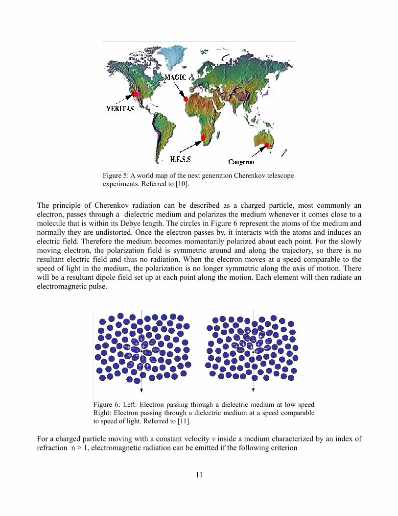
The principle of Cherenkov radiation can be described as a charged particle, most commonly anelectron, passes through a dielectric medium and polarizes the medium whenever it comes close to amolecule that is within its Debye length. The circles in Figure 6 represent the atoms of the medium andnormally they are undistorted. Once the electron passes by, it interacts with the atoms and induces anelectric field. Therefore the medium becomes momentarily polarized about each point. For the slowlymoving electron, the polarization field is symmetric around and along the trajectory, so there is noresultant electric field and thus no radiation. When the electron moves at a speed comparable to thespeed of light in the medium, the polarization is no longer symmetric along the axis of motion. Therewill be a resultant dipole field set up at each point along the motion. Each element will then radiate anelectromagnetic pulse.

For a charged particle moving with a constant velocity v inside a medium characterized by an index ofrefraction n > 1, electromagnetic radiation can be emitted if the following criterion

11

Figure 5: A world map of the next generation Cherenkov telescopeexperiments. Referred to [10].

Figure 6: Left: Electron passing through a dielectric medium at low speedRight: Electron passing through a dielectric medium at a speed comparableto speed of light. Referred to [11].

v c / n (1)

is satisfied according to [12], where c is the velocity of light in vacuum. The index of refractiondepends on frequency which means that the condition can only hold for a finite range of frequencies,typically in the optical range.

The emission of Cherenkov light can be described by the superposition of spherical waves usingHuygen's principle. The resulting cone-shaped wavefront is similar to the shock wave produced bysupersonic jets.

As seen in Figure 7, the radiation is only observed in a characteristic cone with a particular angle φbetween the particle velocity and the emission direction.

The Cherenkov angle φ then can be computed as the following:

cos = c /n t c t

= 1 n

with = vc (2)

The particle emits Cherenkov light while v > c / n (β > v / c), so the minimal velocity for a givenrefractive index n is calculated by:

vmin = cn (3)

or

min = 1n (4)

12

Figure 7: Huygens Construction ofCherenkov radiation. Referred to [13].

For β = 1, the maximum Cherenkov angle is given by the following equation as:

max = arccos1n (5)

As a consequence of the height dependence of the index of refraction, θ increases with the decreasingheight. In the atmosphere at ground level with n = 1.00029, the maximum radiation angle can becalculated as φmax= 1.38º.

For Cherenkov radiation that happens at an altitude of 10 km above the sea level, the light is spreadingover a large area on the ground, typically a circle with a diameter around 250 m.

The minimum energy for a charged particle with rest mass m0 to emit Cherenkov light could becalculated as:

Emin =m 0⋅c

2

1− 1n2

(6)

According to [12, p.389], the number of photons dN emitted per unit path length dz of a particlesatisfied the following condition as:

dNdz

~ 1137

(7)

Condition 7 implies that in a distance of 137 wavelengths, one photon is emitted. In the visiblespectrum, where λ ~ 10-5cm, about 103 photons/cm are emitted.

2.3 Hadronic and Gamma-ray Air ShowerAn air shower is an extensive cascade of ionized particles and electromagnetic radiation produced inthe atmosphere when a primary cosmic ray with extremely high energy enters the Earth. The energy ofthe primary particles are converted all the way to the secondary particles. The process of multiplicationcontinues until that the mean energy of the particles is unable to create more in the subsequentcollisions. Only a small part of the particles will fall down on the ground level. The number depends onthe energy and type of the incident particle.

γ- induced air shower

For every thousand air showers there is one gamma-ray initiated. In this case, the particles producedwould be purely electromagnetic (see Figure 8). Gamma-rays interact with the atmosphere and theirenergy is converted via the following three main processes during the development of air showers:

13

14

Figure 8: CORSIKA simulations of air shower developments in theatmosphere. Left: Electromagnetic air shower induced by 100 GeV gamma-ray. Right: Hadronic air shower induced by 100 GeV primary proton, whichare much less concentrated and spread over a volume larger than for anelectromagnetic shower. Referred to [14], F. Schmidt, "CORSIKA ShowerImages".

➢ Pair production: The photon is converted into an electron-positron pair in the strong field of anucleus: γ → e¯ + e+

➢ Bremsstrahlung: If the energy is sufficient, the resulting electron-positron pair emit gamma rayswhen they pass through the atmosphere: e¯ + e+ → γ

➢ Photoproduction: The cross section of photon production increases with the increasing photonenergy, but is still 300 times smaller than that of pair production: γ + nucleus → hadrons

If the secondary gamma rays have enough energy, they will create another electron/positron pair whichwill undergo further Bremsstrahlung interactions. Therefore, the result of a gamma-ray induced airshower is a cascade of high energy secondary photons, electrons and positrons. All the particlescontinue to travel along the original direction of the primary gamma ray and share its total energy. Mostelectrons and positrons have velocities faster than the velocity of light, thus yielding the Cherenkovradiation.

Hadron-induced air shower

A high energy proton collides with a nucleus in the air creating large number of secondary particles.About 90% of these particles are pions, 10% kaons and anti-protons.

With a short lifetime (τπ0≈ 8.3 · 10-17 s), the neutral pions decay immediately into two photons beforeinteraction: π0 → γ + γ

The energetic photons then create electromagnetic showers. In a cascade of multiple hadronicinteractions a large fraction of the primary energy is eventually transformed into the electromagneticshower components.

The charged pions have a longer lifetime (τπ± ≈ 2.6 · 10-8 s), so they could interact with another nucleusbefore decaying into muons and neutrinos: π+ → μ+ + υμDue to their long lifetime (τµ ≈ 2.2 · 10-6 s) and small interaction cross section, most of the muons areable to reach the ground. Together with the neutrinos these muons remove part of the shower energy.

Consequent processes are similar to the primary interaction and will lead to a cascade of secondaryparticles called hadronic shower.

Therefore a hadron-induced air shower consists of three components:

➢ Hadronic air shower generated by the interaction of charged pions and atmosphere.

➢ A set of electromagnetic sub-showers mainly originating from the π0 decaying.

➢ A fraction of muons and neutrinos

2.4 Detecting Air Showers with Imaging Air Cherenkov TelescopeWhen a high energy particle interacts with the atmosphere, it could initiate an air shower. The electronsand positrons produced within the air shower emits Cherenkov light which can be detected by animaging air Cherenkov telescope located within the light pool on the ground (as shown in the Figure 9).The mirror of the telescope collects a certain amount of the Cherenkov light and reflects it onto thePMT (photomultiplier tube) camera located in the focal plane of the mirror. The camera is triggered

15

when a light level above a preset threshold is detected within a short integration time. The light level ofall pixels are recorded digitally and the images are analyzed to determine whether it has the expectedcharacteristics of a gamma-ray shower.

High energy gamma-rays that can be recorded by telescopes are relatively rare events. They have to bediscriminated against a cosmic ray background several orders of magnitude more abundant.

The discrimination is based on two factors:

➢ Geometry: the gamma ray images have roughly elliptical shape.

➢ Physics: the hadronic shower images will be more broader and more irregular than the image ofelectromagnetic shower (Figure 8).

As early as 1985, M.Hillas proposed the idea of reflecting the modeling of the image by a two-dimensional ellipse. The parameterization of images was performed in terms of a moment analysis ofthe recorded pixel signal amplitudes. The Hillas parameters are derived from the light distribution inthe camera and can be defined as follows (shown in Figure 10):

➢ Length L : a measure of the length of an EAS, corresponding to the RMS value of the lightdistribution along the major axis of the shower image.

➢ Width W: a measure of the width of an EAS, corresponding to the RMS value of the lightdistribution along the minor axis of the shower image.

➢ Orientation angle α: the angle between the major axis of the shower image and the connectingline from the camera center to the center of gravity of the image.

➢ Size (the image amplitude): light content of the shower.

16

Figure 9: Schematic of detecting gamma rays withCherenkov telescopes. The Cherenkov light is beamed inthe air shower and can be collected with optical detectors.Referred to [15].

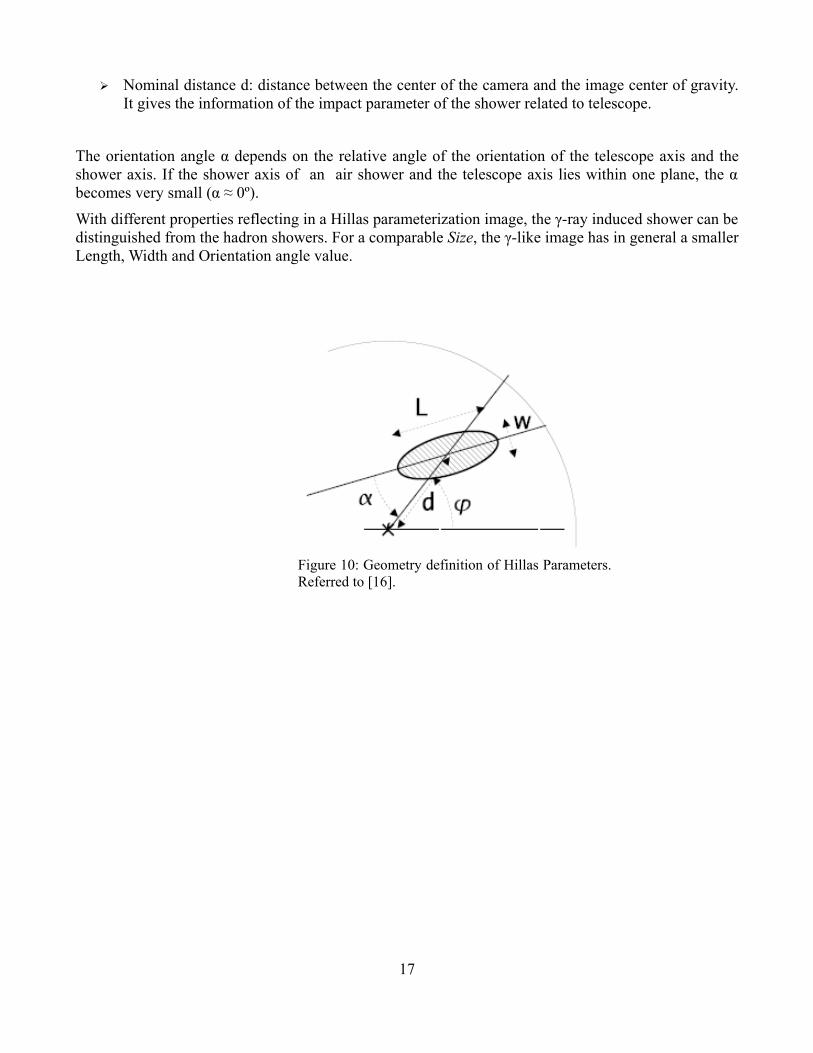
➢ Nominal distance d: distance between the center of the camera and the image center of gravity.It gives the information of the impact parameter of the shower related to telescope.

The orientation angle α depends on the relative angle of the orientation of the telescope axis and theshower axis. If the shower axis of an air shower and the telescope axis lies within one plane, the αbecomes very small (α ≈ 0º).

With different properties reflecting in a Hillas parameterization image, the γ-ray induced shower can bedistinguished from the hadron showers. For a comparable Size, the γ-like image has in general a smallerLength, Width and Orientation angle value.

17

Figure 10: Geometry definition of Hillas Parameters.Referred to [16].

Chapter 3: Reading CORSIKA File

3.1 Monte Carlo SimulationMonte Carlo methods are widely used classes of computational algorithms for simulating the behaviorof various physical and mathematical systems. They are distinguished from other simulation methodsby being stochastic usually by using random numbers.

For understanding of the performance of IACT telescopes like MAGIC, a detailed Monte Carlosimulation of air showers as well as the detector response is required. The simulation must take intoaccount the development of the air showers in the atmosphere, the reflectivity of the mirrors; and theresponse of the photo detectors.

The simulation for a MAGIC -type telescope can be divided into three stages:

➢ The first stage includes simulating the development of gamma-ray and hadron-induced airshowers with CORSIKA (Cosmic Rays Simulation for KAscade), using VENUS model forhadronic interactions and US standard atmosphere. Information of Cherenkov photons arrivingat the observation level contains all their characteristics, such as position, direction andwavelength are stored in binary files.

➢ The second stage of the simulation is the Reflector program, performing the reflection of thephotons hitting the mirror dish onto the camera plane.

➢ The camera program simulates the behavior of the MAGIC photomultiplier camera, triggersystem and data acquisition electronics.

3.2 Analysis ToolsMAGIC Analysis and Reconstruction Software (“MARS”) has been developed for use with theMAGIC telescope, to convert raw data into physics and from FADC output to fluxes. The software isan event-based analysis package developed on the base of the well known ROOT-package [17]. ROOTimplements a large number of basic features and a wide range of tools. MARS is a collection ofdefinitions for basic interfaces, pre-defined algorithms and data structures and can be used for onlineanalysis, standard analysis of data from cosmic sources. Owing to ROOT's C++ interpreter, specificuser-defined analysis tasks can be implemented without the need to recompile MARS. More detailsregarding the structure of MARS can be found in [18].

3.3 CORSIKA 6.500

3.3.1 Introduction

Most of our understanding of the evolution and properties of air showers come from detailed studiesmade with Monte Carlo simulations. CORSIKA (COsmic Ray SImulation for Kascade) [19] is adetailed Monte Carlo program to study the air shower in the atmosphere. It is originally developed toperform simulations for the Kascade experiment [20] at Karlsruhe in Germany, but during the time itbecomes a tool that is used by many groups. Its applications range from Cherenkov telescopeexperiments (E0 ~ 1012 eV) up to giant cosmic ray surface experiments at the highest energies observed

18

(E0 >1020 eV).

CORSIKA 6.500 [21] allows to simulate the interactions and decays of nuclei, hadrons, muons andphotons in the atmosphere up to energies of some 1020 eV. These particles are tracked through theatmosphere until they undergo reactions with the nuclei in the air. The program gives type, energy,location, direction and arrival times of all secondary particles that are created in the air shower and passa selected observation level.

The CORSIKA program is a complete set of standard FORTRAN routines and consists basically fourparts:

➢ The first part handles the input and output, performing decay of unstable particles and trackingof the particles taking into account ionization energy loss.

➢ The second part treats the hadronic reactions of hadrons with air nuclei at higher energies.

➢ The third part simulates the hadronic interactions at lower energy.

➢ The fourth part describes transport and interaction of electrons, positrons and photons.

For latter three parts, CORSIKA contains several models that maybe activated with varying precisionsof the simulations and consumption time of CPU.

3.3.2 Program model options

The hadronic interactions at high energies may be described by the following six reaction modelsalternatively:

➢ HDPM: a set of routines to simulate high-energy hadronic interactions produced byCapdevielle [22] and inspired by the Dual Parton Model.

➢ VENUS: to simulate ultra-relativistic heavy ion collisions.

➢ QGSJET: a quark-gluon-string model using quasi-eikonal Pomeron parametrization for elastichadron-nucleon scattering amplitude.

➢ DPMJET: describe high energy hadronic interactions of hadronic-nucleus and nucleus-nucleuscollisions using two-component DPM.

➢ SIBYLL: simulation hadronic interactions at extreme high energies based on QCD mini-jetmodel.

➢ NEXUS: extensions of enabling a safe extrapolation up to higher energies based on VENUSand QGSJET.

Hadronic interactions at lower energies are simulated with one of the following models:

➢ FLUKA: a package of routines to follow energetic particles through matter by Monte Carlomethod.

➢ GHEISHA: a package that has been proven to describe hadronic collisions up to 100 GeV.

➢ URQMD: to treat low energy hadron-nucleus and especially nucleus-nucleus interactions.

The interactions of electrons and photons can be treated with the shower program:

➢ EGS4: following each particle and its reaction explicitly.

19

➢ NKG: formulas to obtain electron densities at selected locations and the total number ofelectrons at up to 10 observation levels.

Besides the above models, there are several models simulating Cherenkov radiation as well.

➢ Cherenkov Standard Option: The Cherenkov photons are considered within a wavelength bandspecified by the upper and lower limits. It records only the photons at the lowest observationlevel.

➢ Cherenkov Wavelength Option: the index of refraction is made wavelength dependent in theCERWLEN option.

➢ Imaging Atmospheric Cherenkov Telescope Option: routines treating the Cherenkov radiationfor IACT.

➢ Imaging atmospheric Cherenkov telescope extension option: extended by parameters describingthe emitting particle with the IACTEXT option.

➢ Cherenkov light reduction option: with the CEFFIC option, light absorption within theatmosphere, telescope mirror reflectivity are taken into account.

➢ INTCLONG and NOCLONG option: preprocessor option for selecting modes of longitudinaldistribution of photons.

➢ STACEE option: the output of the Cherenkov file is generated in a format used for STACEEexperiment.

In principle, most options can be combined. In this thesis, Cherenkov Standard Option is used. Theroutines treating the Cherenkov radiation is supplied by the HEGRA Collaboration. The Cherenkovlight produced by electrons, positrons, muons and charged hadrons is considered in the subroutinecerenk. By default, atmospheric absorption of the Cherenkov photons is not taken into account. OnlyCherenkov photons arriving at the lowest observation levels are recorded.

More detailed description of CORSIKA program frame, the used cross-sections, the hadronicinteraction model HDMP, the electromagnetic interaction models and the particle decays can be foundin [21].

3.3.3 Data Files

Input

To run a simulation one need to read in several input files [21. p.18]. Besides the data files, CORSIKAneeds the input of steering keywords to select the subject and the parameters of the simulation.

The simulation of the air showers is steered by the keywords in the input card image format. Followingis an input card example including CHERENKOV option of CORSIKA 1999/12/31/cer000001.log

INPUTCARDRUNNR 1PRMPAR 1ERANGE 50 2000EVTNR 1NSHOW 10

20

ESLOPE -3THETAP 2 10PHIP 0 0DIRECT /home/operator/mctest/montecarlo/corsika/1999/12/31SEED 1 0 0 SEED 2 0 0 SEED 3 0 0 OBSLEV 2200.E2RADNKG 200.E2MAGNET 29.5 23.0ECUTS 0.3 0.3 0.02 0.02MUADDI FMUMULT TLONGI T 10. T FMAXPRT 0ECTMAP 1.E4STEPFC 0.1DEBUG F 6 F 1000000CWAVLG 290. 600.CSCAT 1 0. 12000CERSIZ 1.CERFIL TFIXCHI 280DATBAS FCERTEL 1 0. 0. 0. 0. 0. 1800. 1700.USER operatorATMOSPHERE 11 TEXIT

OutputThere are two major output files produced by a simulation run.

➢ Control printout (list file): The simulation run produces a printout that allows to control thesimulation and informs about the general run, the program version with interaction model,steering keywords, physical constants, the atmosphere model and the primary particle.

➢ Particle output file: The particle and Cherenkov photon output files contain information aboutthe simulation run and about all particles reaching observation levels, that to be further analyzedfor detail energy spectra and distributions. By using the keyword CERFIL and setting itsparameter LCERFI to true, two separated data files “DATnnnnnn” and “CERnnnnnn” which isthe output of normal particles and of the Cherenkov photons respectively, can be obtained. The“DATnnnnnn” contains the information of all the particles in the list (see [21]) that reach theground level.

The Cherenkov photon output files are structured as shown in Table 2.

21

Table 2: Block structure of Cherenkov photon output files. Referred to [21].

Run Header Event Header 1 Data Block 1 Data Block 2 ...... Event End1

Event Header 2 Data Block 1 Data Block 2 ....... Event End2

Event Header nevt Data Block 1 Data Block 2 ...... Event End nevtRun End

22

Table 3: Structure of the run header sub-block. Referred to[21].

Run Header sub-block (once per run)Number ofword

Contents of word ( as real number R*4)

1 'RUNH'2 Run number3 Date of begin run(yymmdd)4 Version of program5 Number of observation levels5 + i Height of level i16 Slope of energy spectrum17 Lower limit of energy range18 Upper limit of energy range19 Flag for EGS4 treatment20 Flag for NKG treatment

21 Kinematic energy cutoff for hadrons 22 Kinematic energy cutoff for muons 23 Kinematic energy cutoff for electrons24 Kinematic energy cutoff for photons

Physical constants and interaction flags24 + i C(i), i=1, 5074 + i 0, i=1, 2094 + i CKA(i), i=1, 40......264 + i CATM(i), i=1, 5270 NFLAIN271 NFLDIF272 NFLPI0+100* NFLPIF273 NFLCHE+100*NFRAGM

23

The information is stored unformatted in a fixed block structure with a block length of 22932 bytes[21]. A block consists of 5733 words, each 4 bytes long. Each block consists of 21 sub-blocks of 273words. The sub-blocks are Run Header, Event Header, Data Block, Event End and a Run End sub-block. All quantities are written as single precision real numbers. Structure of other sub-blocks can befound in appendix A.

3.4 AlgorithmAlgorithm of C++ binary file I/O

A binary file is a computer file that may contain any type of data, encoded in binary form for computerstorage and processing purposes. Usually binary files are treated as sequences of bytes.

Input and output with files in C++ are usually performed by using objects of the fstream classesprovided in its standard library:

➢ ifstream: stream class to read from files

➢ ofstream: stream class to write to files

➢ fstream: stream class for both reading and writing from/to files

All these classes are derived from the classes istream and ostream and defined in <fstream.h>.

File stream classes are designed such that a file is viewed as a stream or array of uninterpreted bytes.Each file has two positions:

➢ The current reading position, which is the index of the next byte that will be read from the file.This is called as “get pointer” since it points to the next character that the get method willreturn.

➢ The current writing position, which is the index of the byte location where the next byte will bereplaced. This is called as “put pointer” since it points to the place where the put method willplace its parameter.

These two file positions are independent from each other.

Generally, there are several steps for reading in a file:

➢ Open the file: A file stream can be opened by the “open ” method by supplying a file namealong with an i/o mode parameter to the constructor when declaring the object. In order tomanipulate binary files, the i/o mode as well as mode flags should be always specified.

➢ Check opening error: An opening may fail if the user has wrong permissions or the files donot even exist. So after opening the file, the file objects should be tested to make sure the file isproperly opened.

➢ Reading from the file: Once a file has been successfully opened, one can read from or write toit by using standard I/O commands. To read from a stream object, read (char*, int ) method isused. This method takes two parameters: istream& read(char*, int). The read member functionextracts a given number of bytes from the given stream, placing them into the memory pointedby the ' char* '. The read method does not assume anything about line endings, neither does itplace a null terminator at the end of the bytes that are read in. In case of an reading error, thestream is placed in an error state. All future read operation will fail if a stream goes into an error

24

state.

➢ Repositioning the pointer: The seekg method can be used to change the file reading positionof the 'get' pointer of a stream object. The method moves the 'get' pointer to the specifiedabsolute file position. It also allows to specify a position relative to the current 'get' pointerlocation, or relative to the end of the file.

➢ Close the file: When the reading is done, files must be closed by using the member functionclose. It is important to do this step since the output sometimes is buffered.

Implemented in MARSTo read in CORSIKA binary files, the algorithm (source code in appendix B) is implemented in thecorresponding class of the "mraw" directory of MARS.

➢ Directory mraw: raw data classes for storing the information from raw data files.➢ Class MRawRead: task to read the raw data binary file.➢ Class MRawRunHeader: storage container for general information➢ Class MRawEvtHeader: parameter container for raw event header➢ Class MRawEvtData: container to store the raw event data.

In the MRawRead class, there is a member function called “ReadEvent” that reads one event from theCORSIKA binary file. It calls the member function within the class MRawRunHeader,MRawEventHeader, MRawEventdata to read in the corresponding binary file of Run Header, EventHeader, Cherenkov Photon Data.

The execution of the program for reading in one event is as following:

MRawRunHeader → ReadEvent

MRawEvtHeader → ReadEvent

MRawEvtData → ReadEvent

MRawEvtHeader → ReadEnd

3.5 ResultsParts of the reading file results with the corresponding input card information are as following:

================================================= ReadDaq - MARS V<cvs> MARS - Read and print daq data files Compiled with ROOT v5.12/00f on <Jul 25 2007>

Open the file '/home/operator/mctest/montecarlo/corsika/1999/12/31/cer000001'Preprocessing... MRead [MRawFileRead]... MPrint... PrintEvtHeader [MPrint]... PrintTime [MPrint]...PrintEvtData [MPrint]... PrintEvtData2[MPrint]...

25

Eventloop running (all events)...RunNumber: 1Date Begin: 70521Program Ver: 6.5Slope: -3Emin: 50Emax: 2000Reinit... MRead... MPrint... PrintEvtHeader... PrintTime... PrintEvtData... PrintEvtData2...EventNumber: 1Particle ID : 1Total Energy: 431.186Starting Altitude: 280Number of First Target: 0Height of First Interaction: 829867Momentum in X direction: 27.0298Momentum in Y direction: 0Momentum in Z direction: 430.336Zenith Angle: 0.0628065Azimuth Angle: 0

printing from Cherenkov photon data blockParticle number: 301342X Position: 1185.94Y Position: -584.275U Direction: 0.0647998V Direction: -0.00106319Interaction Time: 26566.9Height of Bunch: 808692

printing from Cherenkov photon data blockParticle number: 301356X Position: 354.069Y Position: -956.171U Direction: 0.0633998V Direction: -0.00170524Interaction Time: 26565.2Height of Bunch: 808231

printing from Cherenkov photon data blockParticle number: 301506X Position: 241.037Y Position: -999.981U Direction: 0.0632089V Direction: -0.0017797Interaction Time: 26565Height of Bunch: 808226

26

(more ......)

According to the parameter setting of the input card, this is a gamma-ray (particle identification as 1)initiated air shower simulation. With the energy ranging from 50 GeV to 200 GeV. the primary particleinteracts with the atmosphere and generates numerous Cherenkov photons. The information of totalenergy, position and direction of all the Cherenkov photons as well as other secondary particles aregiven in the data blocks.

After reading in the CORSIKA file, a parameter container “MRawChePhoton” is created for storing allthe Cherenkov photon data. In MARS, a parameter container is a class inherited from MParContainerand can be added to the parameter list MParList. In class “MRawChePhoton”, method “CreateVectors”is implemented to form the three-dimensional vectors for describing the direction and position of eachphoton.

27

Chapter 4: Reflector Simulation

4.1 IntroductionA reflecting telescope (reflector) is an optical telescope which uses a combination of curved mirrors toreflect light and form an image. Generally, a reflector fulfills two purposes: to increase the efficiency ofthe instrument by deflecting light and to create specific patterns and qualities by redirecting light.

Parabolic reflector

A parabolic reflector, known as a parabolic dish or a parabolic mirror, is a reflective device, commonlyformed as the shape of a paraboloid revolution, a type of surface in three dimension described by thefollowing equation (for elliptical paraboloid opening upward) as:

xa

2

yb

2

= z (8)

With a = b, it becomes a paraboloid of revolution with a minimum point shown in Figure 11:

The parabolic reflector functions according to the geometric properties of the paraboloid shape: if theincidence angle to the inner surface of the reflector equals to the reflection angle, any incoming raywhich is parallel to the main axis of the reflector will be reflected to the focal point of the reflector.Cherenkov photons coming from space and hitting the mirror can be treated as parallel rays, whichwill give a great concentration of light in a tight beam at focus. Many types of energy such as light,sound or radio waves can be reflected in this way. The most common applications of parabolic reflectorare in satellite dishes, telescopes and so on. Larger parabolic reflectors project more light, making themideal for applications that are not restricted by available installation space.

Parabolic reflectors suffer from an aberration called coma which is of primary interest in the telescopeapplication because it requires sharp resolution of the axis. In a parabolic telescope system, there willbe a large amount of coma appearing in images that lie a short distance to one side of the axis. Lightfrom a point source in the center of the field is perfectly focused at the focal plane of the reflector.However, when the light source is off-axis, different parts of the mirror do not reflect the light to thesame point which results in a point of light that is not in the center of the field appearing wedge-shaped.

28

Figure 11: Paraboloid of revolution.Referred to [23].

The further off-axis, the worse this effect will be. Various suggestions have been made for thecorrection of coma.

Spheric reflector

With a curved reflective surface, which may be either convex or concave, most curved mirrors havesurfaces that are shaped like a part of a sphere (see Figure 12).

If a light source is placed in the center of a spherical reflector, all of the rays will be reflected back 180degree of their origin trajectory. Spherical reflectors are the simplest to make and also it is the bestshape for general-purpose use. However, it suffer from spherical aberration. Parallel rays in this casedo not focus to a single point. A parabolic reflector can do a better job for the parallel rays such as thosecoming from a distant object.

4.2 MAGIC ReflectorMAGIC is one of the second generation Cherenkov telescopes with the aim to fill in the observationgap between 10 GeV and 250 GeV, which are the upper limit of space-based detectors and the lowerlimit of ground-based detectors, respectively. Lower energy air showers emit even faint Cherenkovlight in the atmosphere and therefore requiring a more sensitive instrument. That is the reason ofbuilding a big reflecting mirror, trying to collect as much light as possible. The overall reflector shapeof MAGIC is axially-symmetrical parabolic in order to minimize the time spread of the Cherenkovlight flashes in the camera plane. The preservation of the time structure of Cherenkov pulses isimportant for increasing the signal to noise ratio with respect to the night sky background. For theconstruction of such a big parabolic shape, MAGIC collaboration segmented the mirror into 956 smallelements of 0.495 m × 0.495 m covering a total area of 236 m². The individual mirror is a sandwich ofaluminum honeycomb on a 5 mm plate of alloy (see Figure 13). The aluminum plate is diamond-milledto achieve a spherical reflecting surface with a radius of curvature that is more adequate for its positionin the paraboloid. The reflecting surface is divided into several zones with different radii of curvature tomatch the shape of the dish. The front plates are coated against aging after the diamond milling. All themirrors are grouped onto panels and each panel can be moved by an active mirror control system. A

29

Figure 12: Left: Parabolic reflector. Referred to [24].

Right: Spherical reflector. Referred to [25].

large, high-resolution, dynamic range CCD camera is mounted on the mirror frame in a position thatallows simultaneous measurements of focal plane of camera and of the corresponding portion of thesky. For a measurement, the telescope is directed at a point-like source and the CCD simultaneouslyrecords the direct light spot and its reflection from the disk in the focal plane [26].

4.3 Algorithm The reflector of the dedicated IACT is a f/D =1 telescope with a focal length of 17 meters, MAGIC-type reflector.

Simulation steps:

Step 1: define the incident vector

The data obtained in CORSIKA of the Cherenkov photons are:

➢ x position➢ y position➢ u direction cosine to x axis➢ v direction cosine to y axis

Those data describe the trajectory of the incoming photons and are relative to the coordinate origin ofthe reflector on the ground. The prime task is to define the corresponding incident vectors.

The point-direction form for calculating the equation of a line is chosen as:

30

Figure 13: Exploded view of the mirror surface.Referred to [26]. MAGIC mirrors are made ofAlMgSi1.0 plates 5 mm thick, machined to a sphericalshape and polished by diamond milling. The plates areglued together with a honeycomb inside a Al box.

x−x0

u=

y− y0

v=

z−z0

w (9)

As shown above, it is the best way to describe in terms of vectors, to get the incident line in three –dimension space, where the vector(u,v,w) in the equation are the direction cosines pointing in thedirection of the line.

Direction cosines are defined as:

u = cos (10)

v = cos (11)

w = cos (12)where the three angles α, β and γ, are called the direction angles shown in the Figure 14 respectively.The direction cosines, u, v and w represent the cosines of the angles formed between the vector and thethree coordinate positive directions.

They satisfy the equation as:

cos 2cos 2cos 2 = 1 ⇔ u2 v2 w2 = 1 (13)

The value of w is chosen as the following expression:

31

Figure 14: Illusion of vector space.Referred to [27].

w = −1−u2−v2 (14)since the angle between the positive z coordinate and the photon ray is always larger than 90º.

With Equation 9, the incident line of the photon passing through the incident point on the ground canbe obtained as:

x = uw⋅z x0 (15)

and

y = vw⋅z y0 (16)

where z0 = 0.

Step 2: define the equation of reflectorThe dish's surface formed by rotating a parabolic curve about its axis is called a paraboloid ofrevolution. The equation of the reflector as a paraboloid of revolution in the Cartesian coordinatesystem (shown in the Figure 11 with the z- axis as the axis of symmetry), is:

x2 y2 = 4⋅f⋅z z0 (17)where the distance f is the focal length as 17 meters in this case. Choose the vertex (0, 0, 0) of thereflector as the origin of the coordinate system.

Step 3: calculate the intersection point

Firstly check if the photon hits the mirror surface by using the 17 meters radius to see if the incomingline is within the circle. If the photon is on the mirror, with Equation 15, 16 and 17 the two intersectionpoints on the paraboloid can be calculated. The three equations can be solved by using MATLABprogram. Two solutions are obtained and the one with a higher z value is disregard. The intersectioncoordinate (xi, yi, zi) are shown respectively:

x =u

u2v2⋅2pw− y0 v−x0 u−4p2 w2−4pw y0 v−4pw x0 u2y0 v x0 u−u2 y0

2−v2 x02 x0 (18)

y =v

u2v2⋅2pw− y0 v− x0u−4p2 w2−4pw y0 v−4pw x0 u2y0 v x0 u−u2 y0

2−v2 x02 y0 (19)

z =1

u2v 2⋅2pw−y0 v−x 0 u−4p2 w2−4pw y0 v−4pw x0 u2y0 v x 0 u−u2 y0

2−v 2 x02w (20)

32

The equations have a solution even if the photon does not hit the reflector. Most of the data will beneglected because the intersection point is beyond the reflector scope.

Step 4: define the tangent plane and normal vectorThe definition of tangent plane and normal line for a specific surface is: suppose the surface S has anonzero normal vector N at the point P. Then the line passing through P parallel to N is called thenormal line to S at P and the plane through P with normal vector N is the tangent plane to S at P.Suppose S is a surface with the equation

F x , y , z = C (21)and p(a, b, c) is the point on the surface where F is the differentiable, then the equation of the tangentplane to S at P is:

Fxa , b , c⋅x−a F y a , b , c⋅y−bF za , b , c⋅z−c = 0 (22)and the normal line to the surface at P is (parametric form):

x = aFx⋅a , b , ct (23)

y = bF y⋅a , b , ct (24)

z = cF z⋅a , b , ct (25)And the differential (also known as the normal vector) of the reflector defined as 17 is:

vn = 2xi ,2y i ,−4f (26)So the tangent plane and normal line at incident point (xi, yi, zi) on the reflector inner surface can becalculated respectively as:

2xi⋅x−x i 2yi⋅ y− y i −4f ⋅z− zi = 0 (27)

x−x i2xi

=y− yi

2y i=

z− zi−4f (28)

Step 5: calculate the reflecting vectorOnce the light has been reflected from a reflective surface, the angle at which the light departs from thesurface is called the angle of reflection. This angle is measured from a perpendicular to the reflectingsurface to the departing ray of light and is always equal to the incident angle. So the reflecting vectorcan be obtained from rotating the incident vector 180° around the normal vector.

In the ROOT package, “TVector3” [28] is a general three vector class which can be used for thedescription of different vectors in three-dimensions. Together with “TRotation”[29], a class describinga rotation of objects of Tvector3 class, rotating a three dimension vector can be calculated by accessingthe member function as the following:

33

vr = vi .RotateTMath: : Pi , vn (29)

Step 6: obtain the reflecting line

After the rotation around the normal, the three dimensional reflecting vector (also as direction cosines)

vr = xr , yr , zr (30) is obtained. The reflection line can be calculated by the equation:

x−x ixr

=y− yi

yr=

z− zizr

(31)

Step 7: define the focal plane

The focal plane of the reflector can be defined as:

z = 1 7 m (32)

Step 8: draw the plotThe reflection vector intersects with the focal plane, therefore the projection of the photons within the5° field of view can be plotted. The distribution of the Cherenkov photons hitting on the camera can beobtained.

All the calculations above are done in the class “MRawReflector”. The object is passed to the memberfunction CalcReflection. If the photon is on the reflector, MRawChePhoton's direction vector outputwill now change to the reflected direction and the position vector output will change to the position ofthe intersection of focal plane. If the photon is within the field of view on the focal plane, the data ofthe photon will be saved to an parameter array. If the photon is not on the reflector, no record will bemade.

4.4 Results and DiscussionThe mathematical definition of the reflector are already explained. Simulation of different real muonevents and comparison with previous MAGIC reflector results will be presented in this section.

As discussed before, CORSIKA program could simulate several different particles event. Here muon ischosen because of its storage ring which is easy to be distinguished.

All the data of position of muons that hit on the camera will be saved into a text file, which will beloaded into MATLAB program to plot the distribution of muons for every event on the focal plane.The experimental results will be compared with the MAGIC reflector program data.

Set the parameters of the input card to simulate the parabolic reflector as well as the MAGIC reflector:➢ Simulation run number: 06001➢ Particle Identification: 6 (muon)➢ Energy Range: 10 – 20 GeV➢ Slope: -2

34

All the events simulated here are chosen randomly within the run.

Choose the simulation run number as 06001. Fig.15 gives the simulation result of event 1 with bothMAGIC reflector (upper) and user-defined parabolic reflector (down). The FOV of MAGIC is 0.60°while the FOV of the parabolic reflector is 5°. The first event as well as event 7 and 10 shown in Fig.16 and 17 respectively, all give the result as a complete muon ring with a shadow.

35

Figure 15: Comparison of the simulation result of event 1 with MAGICreflector. Up: Real muon event simulated with MAGIC from run 60010. Afull muon ring inside the mirror is shown. Down: distribution ofCherenkov photons induced by muon on the focal plane.

36

Figure 16: Comparison of the simulation result of event 7 with MAGICreflector. Up: Real muon event simulated with MAGIC from run 60010. Afull muon ring inside the mirror is shown. Down: distribution of Cherenkovphotons induced by muon on the focal plane.

The following events give part of the muon ring constructing in the reflector.

37

Figure 17: Comparison of the simulation result of event 10 with MAGICreflector. Up: Real muon event simulated with MAGIC from run 60010. A fullmuon ring inside the mirror is shown. Down: distribution of Cherenkovphotons induced by muon on the focal plane.

38

Figure 18: Comparison of the simulation result of event 2 with MAGICreflector. Up: Real muon event simulated with MAGIC from run 60010. Afull muon ring inside the mirror is shown. Down: distribution ofCherenkov photons induced by muon on the focal plane.

39

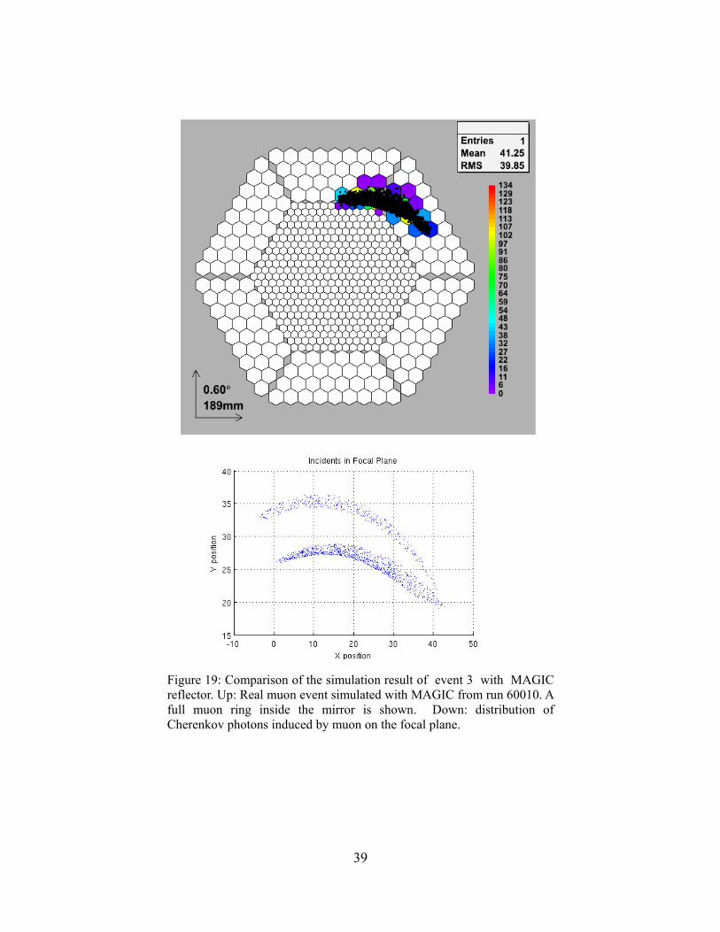
Figure 19: Comparison of the simulation result of event 3 with MAGICreflector. Up: Real muon event simulated with MAGIC from run 60010. Afull muon ring inside the mirror is shown. Down: distribution ofCherenkov photons induced by muon on the focal plane.

40

Figure 20: Comparison of the simulation result of event 4 with MAGICreflector. Up: Real muon event simulated with MAGIC from run 60010. Afull muon ring inside the mirror is shown. Down: distribution ofCherenkov photons induced by muon on the focal plane.

41

Figure 21: Comparison of the simulation result of event 5 with MAGICreflector. Up: Real muon event simulated with MAGIC from run 60010. Afull muon ring inside the mirror is shown. Down: distribution ofCherenkov photons induced by muon on the focal plane.

42

Figure 22: Comparison of the simulation result of event 8 with MAGICreflector. Up: Real muon event simulated with MAGIC from run 60010. A fullmuon ring inside the mirror is shown. Down: distribution of Cherenkovphotons induced by muon on the focal plane.

Comparing the muon events in the user-defined reflector and the MAGIC reflector one can easilymatch the results of muon ring with the corresponding events. There are some important pointsregarding the algorithm needed to be discussed.

➢ The mathematic model of the user-defined algorithm is based on the geometry of the reflectorwhile the former reflector algorithm is more relying on stochastic methods, such as histogram,random numbers. The new method could be used in any reflector due to its modular property.Different parameters or other properties could be easily implemented in the header file class.

➢ There are several photon data in CORSIKA file given both of its direction cosines u and v as 0.And it causes computational errors when calculating the intersection point using Equation 18,19and 20. In this case, the photons that hit on the center of reflector are excluded in the finalfigure. However, it will not affect the results in this work.

➢ The lead time time for a complete whole run includes reading data from CORSIKA file andcalculating with the algorithm and then writing file is around 10 minutes which is reasonablefor such a data processing program.

43

Chapter 5: Conclusion and Future workIn this work, a new modular method for a user-defined reflector for Cherenkov photons in the MARSenvironment is developed. The method has three main parts. First reading data file of Cherenkovphotons with CORSIKA program to get the position and direction vector of all the particles.

Then the reflection of Cherenkov photons (muon in this case) produced by CORSIKA, at a parabolicreflector is simulated and implemented into the MARS environment.

In order to give the final image result, all the data after calculation are saved and written to data filesand exported to MATLAB program.

From the comparison of the simulations showed above, the algorithm has comparable results to theMAGIC reflector, proving that the algorithm is correct.

The running time for calculating all the data within one COSIKA file (one run) is reasonable.

For future work, further components of the reflector could be included, such as: absorption of the entirewindow of the camera, reflection of the light guides.

44

Reference List

[1] http://wwwmagic.mppmu.mpg.de/ collaboration / index.html Updated 12.Apr, 2006

[2] Barrio J.A. Et al. ”The MAGIC telescope Design report” 1998, MPI institute Report MPI-PhE/98-5 (March 1998).

[3] Karl Mannheim. Et al. ”Long term VHE gamma-ray monitoring of bright blazars with adedicated Cherenkov telescope” Letter of intent, February 2007.

[4] http://en.wikipedia.org/wiki/Blazar Updated 30.Dec, 2007

[5] http://www.space.com/images/h_cosmic_jet_000630_03.jpg Refered 27.Apr, 2007

[6] http://www.astronomy.com/asy/objects/images/asy-20020122-01899-orig-lg.jpg Refered27.Apr, 2007

[7] T.C.Weekes. Very high energy gamma-ray astronomy. Physics Reports.160: 1-121, March 1988.

[8] The third EGRET catalog of high energy gamma-ray sources, The Astrophysical journalsupplement series, 123:79-202, 1999 July.

[9] J.V. Jelley, Cherenkov Radiation and its application, Pergamon, New York, 1958.

[10] http://www-hess.desy.de/pics/misc/world_hess.gif Refered 10.May,2007

[11] http://www.sadjadi.org/Cerenkov/theory.htm Refered 10.May, 2007

[12] Julian Schwinger, Lester L.DeRaad, Jr. Kimball A.Milton Wu-yang Tsai,ClassicalElectrodynamics, Massachusetts, 1998.

[13] http://www.pit.physik.uni-tuebingen.de/jochum/dbd/Cherenkov.png Refered 13.May, 2007

[14] F.Schmidt, “CORSIKA Shower Images”, http://www.ast.leeds.ac.uk/~fs/showerimages.html

[15] http://www.dur.ac.uk/~dph0www4/images/detection.jpg Refered 18.May, 2007

[16] http://www.mpihd.mpg.de/hfm/HESS/public/publications/Conf_Palaiseau_2005/deNaurois.pdf

[17] http://root.cern.ch/ Refered 31.May, 2007 Updated 14.Jun,2006

[18] http://magic.astro.uni-wuerzburg.de/mars/ Updated 03.Sep, 2007

[19] http://www-ik.fzk.de/corsika/ Updated 12.Jan, 2008

[20] T.Antoni et al.(KASCADE Collaboration), Nucl.Instr.Meth. A513(2003) 490.

[21] D.Heck, T.Pierog. Extensive Air shower simulation with CORSIKA: a user guide (Version6.500 from March 6, 2006), Forschungzentrum Karlsruhe GmbH, Karisruhe.

[22] J.N. Capdeielle, J. Phys. G: Nucl. Part. Phys. 15, 909 (1989).

[23] http://upload.wikimedia.org/wikipedia/commons/4/40/Paraboloid_of_Revolution.pngRefered 04. Jun, 2007

[24] http://www.pen.k12.va.us/Div/Winchester/jhhs/math/mpage/mgifs/gifs2/para2.jpg Refered04.Jun, 2007

[25] http://www.iatse611.org/html/education/Electrics2_files/image002.jpg Refered 04.Jun, 2007

45

[26] D.Bastieri, C.Bigongiari, N.Galante, E.Lorenz Et al. for the MAGIC Collaboration “Thereflecting surface of the MAGIC telescope”. The 28th International Cosmic Ray Conference.

[27] http://em-ntserver.unl.edu/Math/mathweb/vectors/Image517.gif Refered 5.Jun,2007

[28] http://root.cern.ch/root/html/TVector3.html Updated 19.Nov,2007

[29] http://root.cern.ch/root/html/TRotation.html Updated 19.Nov,2007

46

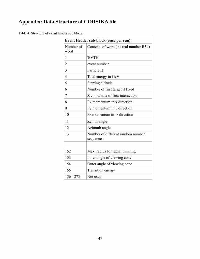
Appendix: Data Structure of CORSIKA file

Table 4: Structure of event header sub block.

Event Header sub-block (once per run)Number ofword

Contents of word ( as real number R*4)

1 'EVTH'2 event number3 Particle ID4 Total energy in GeV5 Starting altitude6 Number of first target if fixed7 Z coordinate of first interaction8 Px momentum in x direction9 Py momentum in y direction10 Pz momentum in -z direction

11 Zenith angle12 Azimuth angle 13 Number of different random number

sequences......152 Max. radius for radial thinning153 Inner angle of viewing cone154 Outer angle of viewing cone155 Transition energy 156 - 273 Not used

47

Table 5: Structure of event end sub block.

Event End sub-block (once per run)Number ofword

Contents of word ( as real number R*4)

1 'EVTE'2 event number3 Weighted number of photons arriving at

observation level4 Weighted number of electrons arriving

at observation level5 Weighted number of hadrons arriving at

observation level6 Weighted number of muons arriving at

observation level7 Number of weighted particles written to

particle output file7 + i i=1, 21 lateral distribution in x direction28 + i i=1, 21 lateral distribution in y direction......265 Weighted number of hadrons written to

particle output file266 Weighted number of muons written to

particle output file267 Number of em-particles emerging from

preshower268 - 273 Not used

Table 6: Structure of run end sub block.

Run End sub-block: (once per run)Number of words Contents of word 1 'RUNE' 2 Run number 3 Number of events processed4... 273 Not used

48

Acknowledgments

Firstly I would like to thank my supervisor Prof. Dr. Karl Mannheim and Dr. Thomas Bretz as well asall my colleagues of MAGIC group for their helpful advice. I appreciate the great help from DieterHeck, the author of CORSIKA, for his quick answers and detailed explanations of all the questions.

Special thanks to Markus Meyer and David Anders Tingdahl for their great support.

49