2004 strengths and limitations of taguchi’s contributions
TRANSCRIPT

Journal of Manufacturing SystemsVol. 23/No. 2
2004
73
Strengths and Limitations of Taguchi’sContributions to Quality, Manufacturing,and Process Engineering
Saeed Maghsoodloo, Dept. of Industrial and Systems Engineering, Auburn University, Auburn, Alabama, USA.E-mail: [email protected] Ozdemir, Dept. of Industrial Engineering, Suleyman Demirel University, Isparta, Turkey.E-mail: [email protected] Jordan and Chen-Hsiu Huang, Dept. of Industrial and Systems Engineering, Auburn University,Auburn, Alabama, USA. E-mail: [email protected]; [email protected]
contributions and present examples to illustrate theapplications of Dr. Taguchi’s methodology to prod-uct and process engineering.
2. Taguchi’s Contributions to QualityEngineering and Design of Experiments
1. Taguchi quantified the definition of Quality us-ing Karl Gauss’s quadratic loss function.
2. He introduced orthogonal arrays (OAs), al-though almost half of them are the classical frac-tional (or factorial) designs developed by SirRonald A. Fisher, G.E.P. Box and J.S. Hunter,F. Yates, O. Kempthorne, S.R. Searle, N.R.Draper, R.L. Plackett and J.P. Burman, J.W.Tukey, H. Scheffé, and countless others.Taguchi’s OAs, however, are already in devel-oped format so that the engineer does not haveto design the experiment from scratch, eventhough the engineer should have some knowl-edge of their development to make proper useof Taguchi’s OAs. In other words, the contri-bution Dr. Taguchi has made in this area is sim-ply making it easier for an engineer to use designof experiments (DOE).
3. Taguchi introduced robust (i.e., parameter andtolerance) designs.
4. He defined a set of measures called signal-to-noise (S/N) ratios that combine the mean andstandard deviation into one measure in analyz-ing data from a robust design.
The following sections will discuss these topicsin the same order as they were introduced above
AbstractThis paper reviews Genichi Taguchi’s contributions to the
field of quality and manufacturing engineering from both astatistical and an engineering viewpoint. His major contribu-tions are first listed and then described in a systematic andanalytical manner. The concepts underlying Taguchi’sunivariate quality loss functions (QLFs), his orthogonal ar-rays (OAs), robust designs, signal-to-noise (S/N) ratios, andtheir corresponding applications to quality and process en-gineering are examined and described in great detail. Someof Taguchi’s OAs are related to the classical (fractional) facto-rial designs (a field that was started by Sir Ronald A. Fisher inthe early 1920s). The applications of Taguchi’s robust (pa-rameter and tolerance) designs to manufacturing engineer-ing are illustrated through designed experiments.
Keywords: Taguchi Methods, Quality Loss Functions, Or-thogonal Arrays, Parameter Design, Tolerance Design, Sig-nal-to-Noise Ratios
1. IntroductionDr. Genichi Taguchi is a Japanese engineer whose
contributions to the field of quality engineering werenot publicized in the Western Hemisphere until theearly 1980s. There have been at least 100 articleswritten on Taguchi methods (a term that was coinedby the American Supplier Institute (ASI), Inc., andone that Taguchi did not greatly admire) in westernjournals in the past 20 years, some very supportiveof his methodology and others critical of his qualityengineering methods. On the other hand, some ar-ticles have fairly and justly evaluated his significantcontributions without any bias. Further, there havebeen many papers on the extension of his method-ology and its applications. The objective in this pa-per is to present an analytical review of his
Journal of Manufacturing SystemsVol. 23/No. 2
2004

Journal of Manufacturing SystemsVol. 23/No. 22004
74
and highlight a few strengths and minor limita-tions of Taguchi’s contributions that have beendebated by the statistical and engineering com-munity. The emphasis will be to illustrate to theprocess engineer how to apply Taguchi methodsand, in general, DOE. Further, for the readers’ con-venience, a comprehensive list of symbols andacronyms is provided under Nomenclature beforethe References section.
3. Taguchi’s Definition of QualityAccording to Taguchi, quality is the amount of
losses a product imparts to society from the mo-ment of shipment. Let X and Y be measurable,static, continuous quality characteristics (QCHs);then a QCH can be of two types: (1) magnitude or(2) nominal. If a QCH is of magnitude type, then Ymay be smaller-the-better (STB), or the QCH Y maybe larger-the-better (LTB), in which case X = 1/Ymust be an STB-type QCH. Thus, when the QCH(such as Y = yield, efficiency, or breaking strength)is LTB, a simple transformation, X = 1/Y, is madeso that X is now STB.
Examples of directly STB QCHs are lateral forceharmonic or eccentricity of a tire, loudness of com-pressors or engines, warpage, and braking distanceof an automobile. All STB static QCHs have two as-pects in common: (1) their ideal target is zero, (2)they all have only a single consumer’s upper speci-fication limit (USL), denoted by yu. In real-life engi-neering applications, when y is an STB QCH itsvalues can never be negative (for example, brakingdistance cannot be negative). Similarly, if the responsey is LTB, then the ideal target is ∞, y > 0, and y hasonly a single lower specification limit, LSL = yL.
Several notable quality gurus (such as W. EdwardsDeming) have alluded to the fact that when a prod-uct barely meets specification, its quality level can-not much differ from one that does not barely meetspecifications. For example, if the design tolerancefor a resistor is 5 ± 0.10 ohm, then there can hardlybe any difference between the quality levels of tworesistors with resistances of 5.099 and 5.101 ohms.However, to the best of our knowledge, GenichiTaguchi was the first quality engineer who recom-mended the use of this very concept (throughGauss’s quadratic loss function) to quantify quality.Accordingly, the quality loss of an item accordingto Taguchi is defined as in Eq. (1).
When y is a nominal dimension, the design (orconsumer’s) specifications are given by m ± �, wherem stands for the midpoint of tolerance range startingfrom LSL = m – � to USL = m + �, and the constant kis always positive. Some authors use � and a few oth-ers use T for the ideal target, but m was used to repre-sent midpoint by Taguchi. Further, Taguchi refers to� as the allowance on either side of the midpoint, m,of tolerance range, while in manufacturing engineer-ing, � is usually referred to as the tolerance (or per-haps the semi-tolerance). Note that we are consideringonly the case of symmetric tolerances, but asymmet-ric tolerances often occur in manufacturing processesand are treated by several authors (see Taguchi,Elsayed, and Hsiang 1989, pp. 30-39; Maghsoodlooand Li 2000; Li 2000). The quality loss functions(QLFs) in Eq. (1) measure how far the dimension of aunit is from its ideal target value m. The farther y de-parts from its ideal target, the larger the QLF becomesexponentially (in powers of 2). The constant k can becomputed immediately once the amount of qualityloss (QL) at a specification limit is known. There isgenerally more information about quality losses at aspecification limit than at any other point in the y-space (due to customer complaints). For example, ifthe 5-ohm resistor with specs 5 ± 0.10 imparts a mon-etary loss of $0.30 at the LSL = 4.90, or USL =5.10 ohms, then 0.30 = k(5 ± 0.10 – 5)2 → k = 30.00$/ohm2. Thus, the QLF for one resistor takes the formL(y) = $30(y – 5)2, and the constant k has convertedthe units of (y – 5)2, which is ohms2, to dollars.Taguchi’s QLF can take into account not only the QLdue to deviation from the ideal target but also all lossesto society (such as repair cost, time loss to the con-sumer, damage to the environment, warranty cost, andall other side effects from the use of the product). Ac-cordingly, depending on what kind of societal lossesL(y) represents, the positive constant k should be com-puted in such a manner that all pertinent societal lossesat a specification limit are taken into account.
Before illustrating an application of the quadraticloss function, suppose that we take a random sampleof size n from a process or from a supplier’s lot. Theloss due to the i-th unit in the sample for a nominal
( )
( )
2
2 2
2
L y
k y , y is an STB type QCH
k / y k x , y is an LTB type QCH, and x is STB
k y m , y is a nominal dimension
=
⎧⎪⎪ =⎨⎪
−⎪⎩
(1)
Journal of Manufacturing SystemsVol. 23/No. 2
2004
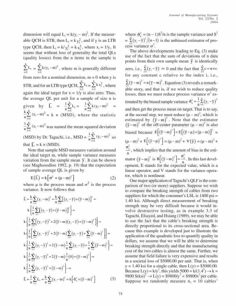
75
dimension will equal Li = k(yi – m)2. If the measur-able QCH is STB, then Li = k 2
iy , and if y is an LTB
type QCH, then Li = k/ 2iy = k 2
ix , where xi = 1/yi. Itseems that without loss of generality the total QLs(quality losses) from the n items in the sample is
n
ii 1
L=∑ =
n2
ii 1
k (y m)=
−∑ , where m is generally different
from zero for a nominal dimension, m = 0 when y is
STB, and for an LTB type QCH, n
ii 1
L=∑ =
n2i
i 1
k x=∑ , where
again the ideal target for x = 1/y is also zero. Thus,the average QL per unit for a sample of size n is
given by L = n
ii 1
1L
n =∑ =
n2
ii 1
1k (y m)
n =−∑ =
n2
ii 1
k(y m)
n =−∑ = k × (MSD), where the statistic
n2
ii 1
1(y m)
n =−∑ was named the mean squared deviation
(MSD) by Dr. Taguchi, i.e., MSD = n
2i
i 1
1(y m)
n =−∑ so
that L = k × (MSD).Note that sample MSD measures variation around
the ideal target m, while sample variance measuresvariation from the sample mean y . It can be shown(see Maghsoodloo 1992, p. 19) that the expectationof sample average QL is given by
E L = k + ( m)2 2( ) −⎡⎣ ⎤⎦σ µ (2)where µ is the process mean and �2 is the processvariance. It now follows that
Lk
ny m
k
ny y y m
kn
y y y m
ii
n
ii
n
i
= −( ) = −( ) + −( )⎡⎣ ⎤⎦ =
−( ) + −( )⎡
= =∑ ∑2
1
2
1
1⎣⎣ ⎤⎦
⎧⎨⎩
⎫⎬⎭
=
−( ) + −( ) −( ) + −( )⎡⎣
⎤⎦
⎧⎨
=
=
∑
∑
2
1
2 2
1
12
i
n
i ii
n
kn
y y y m y y y m⎩⎩
⎫⎬⎭
=
−( ) + −( ) −( ) + −( )⎡⎣⎢
⎤⎦⎥
⎧
= ==∑ ∑∑k
ny y y m y y y mi
i
n
ii
n
i
n12
2
1
2
11⎨⎨⎩
⎫⎬⎭
=
−( ) + −( ) −( ) + −( )⎧⎨
= ==∑ ∑∑k
ny y y m
ny y
ny mi
i
n
ii
n
i
n12
1 12
1
2
11⎩⎩⎫⎬⎭
=
−( ) + −( ) ( ) + −( )⎧⎨⎩
⎫⎬⎭
=
−( )
=∑k
ny y y m
ny m
kn
y y
ii
n
ii
12
10
1
2
1
2
2
==
=
∑
∑
+ −( )⎧⎨⎩
⎫⎬⎭
→
= = −( ) = + −( )⎡⎣
⎤⎦
1
2
1
2 2 2
n
ii
n
i ni
y m
L1
nL
k
ny m k y mσ
==∑
1
n
where σn2 = (n – 1)S2/n is the sample variance and S2
= ∑ −( ) −( )=i
n
iy y n1
21 is the unbiased estimator of pro-
cess variance �2.The above developments leading to Eq. (3) make
use of the fact that the sum of deviations of n datapoints from their own sample mean y is identically
zero, i.e., ∑ −( )=i
n
iy y1
� 0 and the fact that ∑ = ×=i
n
c n c1
for any constant c relative to the index i, i.e.,
∑ −( ) = −( )=i
n
y m n y m1
2 2. Equation (3) reveals a remark-
able story, and that is, if we wish to reduce qualitylosses, then we must reduce process variance �2 es-
timated by the biased sample variance σni
n
iny y2
1
21= ∑ −( )=
and then get the process mean on target. That is to say,at the second step, we must reduce (µ – m)2, which isestimated by y m−( )2
. Note that the estimatory m−( )2 of the off-center parameter (µ – m)2 is also
biased because E y m E y m−( )⎡⎣
⎤⎦ = −( ) + −( )⎡⎣ ⎤⎦
2 2µ µ =
(µ – m)2 + E y −( )⎡⎣
⎤⎦µ 2
= (µ – m)2 + V y( ) = (µ – m)2 +σy
n
2
, which implies that the amount of bias in the esti-
mator y m−( )2 is B y mn
y−( )⎡⎣
⎤⎦ =2
2σ. In this last devel-
opment, E stands for the expected value, which is alinear operator, and V stands for the variance opera-tor, which is nonlinear.
One major application of Taguchi’s QLF is the com-parison of two (or more) suppliers. Suppose we wishto compare the breaking strength of cables from twosuppliers for which the consumer’s LSL is 1400 psi =1.40 ksi. Although direct measurement of breakingstrength may be very difficult because it would in-volve destructive testing, as in example 3.3 ofTaguchi, Elsayed, and Hsiang (1989), we may be ableto use the fact that the cable’s breaking strength isdirectly proportional to its cross-sectional area. Be-cause this example is developed just to illustrate theapplication of the quadratic loss to quantify quality indollars, we assume that we will be able to determinebreaking strength directly and that the manufacturingcost of the two cables is almost the same. Further, weassume that field failure is very expensive and resultsin a societal loss of $5000.00 per unit. That is, wheny = 1.40 ksi for a single cable, then L(y) = $5000.00.Because L(y) = k/y2, this yields 5000 = k/(1.42) Æ k =9800 $(ksi)2 Æ L(y) = $9800/y2 = $9800x2 per cable.Suppose we randomly measure n1 = 10 cables’(3)

Journal of Manufacturing SystemsVol. 23/No. 22004
76
strength from supplied 1 and n2 = 13 from supplier2. In practice, one should allocate more observa-tions to the process that has larger variability. Forexample, if we have total resources of N = 42 itemsto be sampled and we know that �2 = 2�1, then pro-cess 2 must be allocated a sample of size n2 =
σσ σ
2
1 2+⎛
⎝⎜
⎞
⎠⎟ N =
2
3 × 42 = 28, while n1 = 14. Of course,
the experimenter may not have any knowledge ofthe variability of the two processes, in which casethe sampling must be done in (at least) two stages toassess variation at the first stage, followed by com-pleting the sample allocations at the second stage.The two data sets are given below.
y1j : 1.5, 1.4, 1.7, 1.5, 1.6, 1.5, 1.8, 1.8, 1.7, 1.6y2j : 1.9, 1.9, 2.2, 2.5, 1.6, 2.1, 2.0, 1.8, 1.7, 2.5, 2.1, 1.8, 1.5 ksi
It seems that from a traditional view of quality thereare no differences in the quality of the two suppliersbecause neither sample contains a nonconformingunit (that is, all y values � 1.4 ksi). However, basedon the modern view of quality using Taguchi’s QLF,there is much difference between the quality levelsof the two types of cables. Converting to the vari-able x = 1/y, we obtain
x1j : 0.6667, 0.7143, 0.5882, 0.6667, 0.6250, 0.6667, 0.5556,0.5556, 0.5882, 0.6250
x2j : 0.5263, 0.5263, 0.4545, 0.4000, 0.6250, 0.4762, 0.5000,0.5556, 0.5882, 0.4000, 0.4762, 0.5556, 0.6667
Note that x is an STB type QCH with ideal target m = 0.
Then, MSD1 = 1
10 1
102∑
=iix = σx
2 + x( )2 = 0.002553 +
(0.62518674)2 = 0.3934113, where the sample vari-
ance σx2 =
11
2
nx x
i
n
i∑ −( )=
. Then the average quality loss
of supplier 1 is L1 = 9800 × 0.3934113 = $3855.431per cable. Similarly, for the supplier 2, x2 = 0.5193and σ2
2 = 0.005932 → MSD2 = 0.005932 + (0.5193)2
= 0.27558 → L2 = 9800 × 0.27558 = $2700.66673per cable, and hence the quality difference of sup-plier 2 over supplier 1 is QD21 = $1154.7639 percable. This is in complete contrast to zero QD be-tween the two suppliers from the traditional (or con-ventional) quality viewpoint.
The quality engineer should observe that when y isa magnitude type QCH then—unless the coefficientof variation cv xx= ˆ /σ (or variation coefficient, whichis the reciprocal of S/N ratio and is equal to 8.0817%for the sample of supplier 1, and 14.83% for supplier
2) exceeds 30% for an STB QCH and 17% for anLTB QCH—the mean (or the signal) will play a muchmore important role in improving quality than reduc-ing variability (Maghsoodloo 1990). Further, if theQCH values are far above the LSL (for LTB) and farbelow USL (for an STB type QCH), then we can with-stand quite a bit of variation compared with when theoutput values are close to a specification limit. For theabove example on breaking strength, given that thebreaking strength’s LSL = 1.40 ksi, the sample 3.1,5.6, 1.9, 2.8, 7.9 ksi (with variance σ1
2 = 4.81840)implies far superior quality over the sample 1.6, 1.7,1.5, 1.6, 1.7 ksi (with variance σ2
2 = 0.00560). In fact,the QD of the former sample over the latter is equal toQD12 = 3758.7624952 – 1090.795726 =$2667.96677 per cable, but the y-variance of theformer sample is 860.4286 times the y-variance ofthe latter sample, and the x-variance of the formersample is 23.5551 times larger than the latter. (Notethat for x > 1 the transformation x = 1/y is of the vari-ance-reduction type, causing the x-variance of the firstsample to reduce substantially more than that of thesecond sample.)
However, the above assertion cannot be made fora nominal dimension because the process mean µmay be below the ideal target m (in which case thesignal must be increased), or µ may be above themidpoint of tolerances, m, in which case the amountof off-center (µ − m) exceeds 0, and the signal mustbe reduced to improve quality. Further, the processvariance �2 will almost always play an important rolefor a nominal dimension in quality improvement(QI) because the standardized amount of off-cen-ter (µ – m)/� is a truer measure of lack of qualitythan is the off-center distance µ − m .
Relationship Between Natural Tolerancesand Taguchi’s Expected Quality Loss for aNominal Dimension
By definition, if a process is six-sigma capable(that is, process capability ratio PCR = Cp =USL LSL−
6σ = 1), then in the symmetric case the dis-
tance between USL and LSL is exactly six sigma,that is, six-sigma process capability implies that USL– LSL = 6�, which in turn implies that 2� = 6�, or �= �/3. Note that six-sigma capability is different fromMotorola’s definition of Six-Sigma Quality, whereboth the LSL and USL are at six sigma below andabove the process mean µ, respectively.

Journal of Manufacturing SystemsVol. 23/No. 2
2004
77
However, as Montgomery (2001b, p. 24) pointsout, and we concur, there is a slight inconsistency inthis definition when the process becomes off-centeredor is out of control only with respect to its mean. Infact, we think that there is a slight misconception withthis definition when the process is out of control onlywith respect to its mean. The problem arises due tothe fact that the values of LSL = m − � and USL = m+ � are fixed and set by the manufacturing designeror consumer, and consequently, a machining processis either capable of meeting specifications (i.e., p < �)or not capable (i.e., p > �), where p is the processfraction nonconforming (FNC) and � is the company-wide tolerable FNC set in such a manner that the com-pany will prosper in global competition. If the processis centered such that µ = m, the point that we are rais-ing is moot; however, when µ shifts, say by one sigmato the right of m, then it will be impossible for bothLSL and USL to be six sigma away from µ becauseLSL and USL are fixed and do not change as µ shifts.In fact, with an upward shift in µ of one sigma to theright of m, the LSL will be seven sigma to the left ofµ, while the USL will be five sigma to the right of µ.
It would be more prudent to incorporate Taguchi’sview of quality with Motorola’s definition of six-sigma quality and slightly modify Motorola’s six-sigma quality as LSL and USL at six sigma from theideal target m (not µ). Notwithstanding, this modifi-cation will not alter the amount of FNC that a pro-cess produces when only the mean is out of control.For example, when a process is Gaussian and cen-tered (i.e., µ is in control at m) and operating atMotorola’s six-sigma quality, then its FNC is0.00197317540085 parts per million (ppm), orroughly 2 parts per billion. However,
if the mean of a Gaussian process is out of control by 12
sigma (i.e., µ = m ± �/2), its FNC is increased to0.0190297223534586 ppm;
if the mean of a Gaussian process is out of control by 1sigma (i.e., µ = m ± �), its FNC increases to0.28665285167762 ppm;
if the process is off-centered by 1 12 sigma (i.e., µ = m ±
1.5�), then the Gaussian process FNC increases to3.3976731564911 ppm;
if µ = m ± 2�, the FNC increases to 31.671241833786ppm;
if µ = m ± 2.5�, the FNC increases to 232.62907903554ppm;
if µ = m ± 3�, the FNC increases to 1349.898031630096ppm;
if µ = m ± 3.5�, the FNC increases to 6209.66532578 ppm;if µ = m ± 4�, the process FNC increases to
22750.13194818 ppm;if µ = m ± 4.5�, the process FNC increases to
66807.20126886 ppm;and finally, when the mean is way out of control by 5�,
the Gaussian FNC increases to 158655.253931457 ppm(or roughly 0.158655254).
In general, if µ = m ± r � (r � 0), the MotorolaGaussian FNC is given by pM = 2 – �(6 – r) – �(6 +r), where � represents the cdf (cumulative distribu-tion function) of a unit normal distribution.
In practice, the values of process mean and stan-dard deviation, µ and �, are generally unknown andhave to be estimated by the sample statistics y andS, respectively. To ascertain whether a process (pro-ducing a nominal dimension y) is operating atMotorola’s six-sigma quality, one must compute thetolerance interval y ± K S and determine if this tol-erance interval is contained in the tolerance range(LSL, USL). Unfortunately, the values of the toler-ance factor, K, for a tolerable FNC of � = 2 parts perbillion at any confidence probability of � has notbeen reported, as far as we know, in statistical litera-ture. Ms. Hsin-Cheng Chiu (1995) developed a soft-ware that computes the values of K for nearly anysituation, but her program does not allow an � valueless than 0.000001 (= 1 ppm, which pertains toMotorola’s 4.892-sigma quality not 6). For example,for a random sample of size n = 20 from a N(µ, �2),� = 0.000001, � = 0.99, and a nominal dimension y,her program reports K = 7.88, while for n = 30 herprogram gives K = 7.01. Further, the Tolerance Lim-its software reports that a random sample of size atleast n = 83 is needed to obtain a tolerance factor of K� 6 at � = 0.000001 and � = 0.99. Since obtaining theexact tolerance factor to attain Motorola’s six-sigmaquality is not an easy task, it is best to estimate thesample FNC assuming that the process is Gaussian.Thus, the recommendation is first to computeZ LSL y SL = −( ) , ˆ ˆp ZL L= ( )Φ , Z USL y SU = −( ) ,ˆ ˆp ZU U= −( )Φ , and ˆ ˆ ˆp p pL U= + . If ˆ ˆ ˆp p pL U= + is lessthan two parts per billion, then conclude that the ma-chining process is practically operating at six-sigmaquality; otherwise, the process is not operating at six-sigma quality. Further, the experimenter must be cogni-zant that the statistic ˆ ˆp pL U+ is subject to samplingerror and/or fluctuations and the fact that p is lessthan two parts per billion does not guarantee that the

Journal of Manufacturing SystemsVol. 23/No. 22004
78
machining process is operating at Motorola’s six-sigma quality.
To relate the natural tolerances of a normal processto Taguchi’s QLF, the four most common possibilities(out of infinite) are considered, as outlined below:
(i) µ = m and a Six-Sigma Process CapabilityRatio (Cp = 1) Æ USL – LSL = 6�����
E(QL) = k �2 =
Ac
∆2 [(USL – LSL) / 6]2 =Ac
∆2 (2�/6)2 = Ac/9; note that in this case � =
�/3, where Ac is the amount of QL (qualityloss) at either the LSL, or USL. This is in con-trast to the evaluation of quality from a con-ventional viewpoint because if a process issix-sigma capable and is also normally dis-tributed with µ = m, then the amount of tradi-tional QL (based on either meeting or notmeeting specs) is simply 0.0027 × Ac becausethe traditional QL function is given by QLTrad(y)
= 0,
,
if LSL y USL
A otherwisec
≤ ≤⎧⎨⎩
. This implies that the
conventional (or traditional) method of qualityevaluation underestimates quality losses by97.57%.
(ii) µ = m and an Eight-Sigma ProcessCapability Æ USL – LSL = 8�����
→ PCR = 1 33333. and E(QL) = Ac
∆2 [(USL –
LSL) / 8]2 = Ac/16, but E(QLTrad) = 0.0000633425Ac. In this case, the conventional method ofquality evaluation underestimates quality lossesby 99.8986520%.
(iii) µ = m + 0.50����� and a Six-Sigma ProcessCapability Æ USL – LSL = 6�����
E(QL) = k [�2 + (µ – m)2] = Ac
∆2 [(�/3)2 + 0.25
(�/3)2] = Ac (1/9 + 0.25/9) = 1.25 Ac/9, whileE(QLTrad) = 0.0064423 Ac, underestimating QLsby 95.361544%.
(iv) µ = m + 0.50����� and an Eight-Sigma ProcessCapability Æ USL – LSL = 8�����
PCR = 1 33333. → � = �/4 → E(QL) = Ac
∆2 [(�/
4)2 + 0.25 (�/4)2] = 1.25 Ac/16, and E(QLTrad) =
0.00023603 Ac, underestimating QLs by99.6978816%.
In general, if a process is off-centered such that µ– m = r � (r � 0) and PCR stands at t × �, that is, t ×� = 2�, then it can be verified that the E(QL) = 4(1 +r2)Ac/t
2. Further, if a process is Gaussian (that is, nor-mal) and off-centered by r � and operating at a PCR= t �, then the amount of traditional QL is equal toE(QLTrad) = Ac[�(–r – t/2) + �(r – t/2)], where
( ) 2z
–u 2
-
1z e du
2 ∞
Φ =π ∫ is the cumulative distribution
of the standardized (or unit) normal random variable.
As an example, suppose that QI (quality improve-ment) efforts on a machine have improved the pro-cess mean from the off-target value of m + 0.75� toµ = m (i.e., the process has been centered) and theexisting six-sigma process capability (that is, PCR =1) has been improved to seven-sigma process capa-bility, that is, PCR = 7/6. We wish to compute thepercent reduction in Taguchi’s expected societal QLsand also the amount of conventional QI. Before QI,the amount of expected Taguchi’s QL is given byE(QLb) = 4(1 + 0.752)Ac/6
2 = 0.173611 Ac; after QI,E(QLa) = 4Ac/7
2 = 0.081633 × Ac, so that the amountof QI is given by 0.09198 Ac. The conventionalexpected QL before improvement is given byAc[�(–0.75 – 6/2) + �(0.75 – 6/2)] = Ac[�(–3.75)+ �(–2.25)] = Ac[0.00008842 + 0.0122245] =0.012313Ac. After QI, the traditional QL is givenby Ac[�(–0 – 7/2) + �(0 – 7/2)] = 2Ac�(–3.5) =2Ac × 0.000233 = 0.0004653Ac. This yields a con-ventional QI equal to 0.01185Ac, which underes-timates the expected QI by 87.12%.
We have not found articles that are critical of Dr.Taguchi’s use of Karl Gauss’s quadratic loss func-tion to quantify product quality. In fact, Pignatielloand Ramberg (1991) list this contribution as numberfour among Taguchi’s top-10 triumphs. The quadraticloss function discovered by Karl Gauss has been inexistence well over 200 years, but Dr. Taguchi wasthe first who formalized its use to quantify quality,and hence he fully deserves credit for this particularapplication of Gauss’s quadratic loss function.
4. Literature ReviewTaguchi methods have been discussed extensively
in different platforms, such as panel discussions,
Journal of Manufacturing SystemsVol. 23/No. 2
2004
79
books, articles, and so on, especially since the early1980s, when applications to different industries be-gan in the Western Hemisphere. Below is a brief (yetincomplete) summary of these discussions. We willnot discuss every article published in this area in thepast 24 years, but will provide numerous referencesfor the interested reader in the Bibliography section.
Taguchi’s two most important contributions toquality engineering are the use of Gauss’s quadraticloss function to quantify quality and the develop-ment of robust designs (parameter and tolerancedesign). Taguchi’s robust designs have widespreadapplications upstream in manufacturing to fine-tunea process in such a manner that the output is insensi-tive to noise factors. Nearly half of this article dealswith Taguchi’s parameter and tolerance designs.
Several papers about Taguchi methods originatedfrom the Center for Quality and Productivity Im-provement (CQPI) at the University of Wisconsin. Anumber of reports evaluated Taguchi methods froma statistical standpoint. The primary ones are by Boxand Fung (1986); Box, Bisgaard, and Fung (1988);Box and Jones (1992); Bisgaard (1990, 1991, 1992);Czitrom (1990); Bisgaard and Diamond (1990);Bisgaard and Ankenman (1993); and Steinberg andBurnsztyn (1993). In these reports, the parameterdesign received the most attention. These authorsconfirm that Dr. Taguchi has made important contri-butions to quality engineering; however, it may notbe easy to apply his techniques to real-life problemswithout some statistical knowledge. Specifically, theuse of signal-to-noise ratios in identifying the nearlybest factor levels in order to minimize quality lossesmay not be efficient.
Three important discussions on Taguchi methodshave been published in Technometrics by Leon, Shoe-maker, and Kackar (1987); Box (1988); and Nair(1992). Some other performance measures are givenand discussed as alternatives to signal-to-noise ra-tios by Leon, Shoemaker, and Kackar (1987) andBox (1988). Taguchi’s parameter design is discussedextensively by a group of scientists in a discussionpanel chaired by Nair (1992). The scientists’ majorpoint is that Taguchi methods do not have a statisti-cal basis and signal-to-noise ratios pose some com-putational problems.
Shoemaker and Tsui (1991) studied Taguchi’sparameter design from the standpoint of cost. Theyclaimed that putting controllable and uncontrollable
factors in two separate arrays, inner and outer, willresult in more experimental runs. Montgomery(1997, pp. 622-641) highlights the same difficultyin a Taguchi parameter design. We tend to agree withthese authors that more cost may be involved in aTaguchi crossed-array design than in a combinedsingle-array classical design as long as the output iseither an STB or LTB type QCH. When the output isof magnitude type (i.e., QI requires either decreas-ing the signal or increasing the signal), we illustratedabove that unless the CV is larger than 17%, the tra-ditional classical DOE will identify factors that sig-nificantly impact the mean of the output, and thiswill in turn pave the way to improve quality. How-ever, when the output is of nominal dimension, it isbest to invest the extra capital to identify the con-trols (these are the factors that control process varia-tion) and signals (these are factors that impact themean but have negligible effect on variability) andgo through the Taguchi two-step procedure of firstreducing variability followed by getting the meanon target. Thus, our recommendation to any engi-neer is to use DOE by all means as an upstream QItool. If the engineer does not have sufficient re-courses and the QCH is either STB or LTB and theCV < 20%, then use a single-array classical FFDmaximizing design resolution (defined later). If theQCH is of nominal-the-best type, then by all meansuse Taguchi’s parameter design even if more experi-mentation is required. Further, if the noise factorsare environmental variables, it is generally best toplace such variables in an outer array and treat themas uncontrollable. Box and Jones (1992) discuss analternative to a Taguchi crossed-array design whenthe noise factors are environmental.
Tsui (1996) reviews and gives probable problemswith Taguchi methods. He compares Taguchi meth-ods with other alternative approaches in the litera-ture. According to Kim and Cho (2000), it is expensiveto arrive at a process having on-target mean and mini-mum variance with Taguchi methods. They suggestan alternative model based on an asymmetric qualityloss to obtain the most economical process mean.Robinson, Borror, and Myers (2004) in a recent ar-ticle gather previous arguments and alternative ap-proaches to Taguchi methods. Alternative performancemeasures are discussed and are compared with sig-nal-to-noise ratios. Also Taguchi’s parameter designis reviewed from different perspectives.

Journal of Manufacturing SystemsVol. 23/No. 22004
80
It is nearly impossible to discuss all of the worksrelated to Taguchi methods. We have tried to men-tion the main articles that discuss the pros and consof Taguchi’s contributions. There are several otherpapers that are listed in the Bibliography but are notspecifically discussed here.
5. Factorial Designs and Taguchi’sOrthogonal Arrays
Because roughly half of Taguchi’s orthogonal ar-rays (OAs) are related to classical (fractional) facto-rial designs, this section is a short summary offactorial designs that were developed mainly by SirRonald A. Fisher (1966), Kempthorne (1952), Yates(1937), Graybill (1961), Tukey (1949), Cochran andCox (1957), Scheffé (1953, 1956, 1959), Searle(1971a), and other notables. The factorial bk meansthat the design matrix, X, contains k � 2 differentfactors (or process parameters, or k inputs) each at blevels (b = 2, 3, 4, …), contains bk factor level com-binations (FLCs, or treatment combinations), andpossesses exactly k arbitrary columns. The factorialdesign bk, k � 2, is complete (or a full factorial)only if at least one response is obtained at each ofthe bk FLCs. Further, if the number of responses ateach FLC is the same, namely n, then the designmatrix X is also said to be balanced and orthogonal.A matrix X is orthogonal if and only if (XTX) = (XX)is diagonal or can be diagonalized through a lineartransformation, where T and “” stand for transpose.The number “b” is called the design base, and thetotal number of columns of a design matrix will begiven in the following subsection. Before relatingTaguchi’s OA to classical factorial (or fractional fac-torial) designs, general rules will be listed that willapply to all balanced orthogonal fractional factorialdesigns (FFDs) to facilitate the understanding of OAsand how to put them to use in practice.
Review of Fractional Factorial DesignsFractional (or incomplete) factorial designs, or
fractional replicates, were developed mainly by Boxand Hunter (1961a,b), John (1961, 1962, 1964), Friesand Hunter (1980), Kempthorne (1952), Montgom-ery and Runger (1996), and other notables. We nowsummarize the rules that will apply to all balancedand orthogonal FFDs.
1. The notation bk–p means that the design matrix,X, contains k � 3 different factors (or process
parameters, or k inputs) each at b levels (b = 2,
3, 5, etc.), but only the p
1
bth fraction of all pos-
sible bk FLCs (or treatment combinations) areexperimentally tested. For example, the FFD25–2 implies that our design matrix has five fac-tors (A, B, C, D, and E) each at two levels, butonly Nflc = 25–2 = 23 = 8 distinct FLCs out of thepossible 25 = 32 are studied. (Note that Nflc
stands for the number of distinct FLCs that com-prise the design matrix X, and just to simplifynotation, we let Nf = Nflc.) Further, in any de-sign of experiments the grand total number ofobservations in the entire experiment, assum-ing a balanced and orthogonal design, can bewritten as N = n × Nf. Similarly, a 34–1 is a 3–1 =1/3rd fraction of a full 34 factorial design, andhence its design matrix will have Nf = 34–1 = 33
= 27 distinct FLCs (or experimental runs). By a36–2 FFD we mean a 3–2 = 1/9th fraction of acomplete 36 factorial, and only Nf = 81 = 36–2 =34 FLCs out of the possible 729 = 36 FLCs aretested experimentally. The reader should notethat for the case of FFDs the values of the de-sign base “b” have been intentionally restrictedto prime numbers 2, 3, 5, 7, etc., because ofthe fact that direct meaningful fractionalizationin nonprime bases (such as 4 and 6) is impos-sible, at least to the knowledge of the authors.Indirect fractionalization in nonprime bases willrequire the use of pseudo-factors and hence ismuch more laborious to carry out. Further, theFFD bk–p will have exactly (bk–p – 1)/(b – 1) col-umns, only k – p of which can be written arbi-trarily and will have exactly Nf = bk–p distinctnumber of rows (or FLCs, or treatments). Forexample, the design matrix of a 26–2 FFD has(26–2 – 1)/(2 – 1) = 15 distinct columns, four ofwhich are arbitrary, and 26–2 = 24 = 16 distinctrows (or distinct FLCs). While a 36–2 FFD has(36–2 – 1)/(3 – 1) = 40 columns, only 4 (= 6 –2) of which are arbitrary, and its design ma-trix X has Nf = 36–2 = 34 = 81 rows, or distinctFLCs. The complete factorial bk can be frac-tionalized into bp, (p < k – 1, k � 3 ), distinctblocks each containing bk–p runs (or distinctFLCs) for b = 2, 3, and 5.
2. The elements (or factor levels) for a base-b de-sign are simply 0, 1, 2, 3, …, b – 1. Taguchiadds 1 to the elements 0, 1, 2, …, b – 1 to ob-

Journal of Manufacturing SystemsVol. 23/No. 2
2004
81
tain his factor levels as 1, 2, 3, …, b. Thus, inthe classical FFD notation the elements of base2 are 0, 1; the levels of base-3 designs are 0, 1,2; and the elements of base-5 designs are 0, 1,2, 3, 4, while in Taguchi’s designs the levelsare (1, 2), (1, 2, 3), and (1, 2, 3, 4, 5), respec-tively. In base 2 algebra, 2 will equal to 0(modulus 2) and 3 will be referred to as 1 (mod2). Similarly, in base 3 algebra, 3 = 0 (modulus3, or mod 3), 4 = 1 (mod 3), and 5 = 2 (mod 3),etc. For example, a 33 factorial design has 27 =33 distinct FLCs starting with 000 (all three fac-tors at their low levels), 001 (factors A and B attheir low levels while factor C at its mediumlevel), 002 (factors A and B at their low levelswhile factor C at its high level), 010, 011, …,221, and ending with 222 (where all three fac-tors are at their high levels).
3. The degree(s) of freedom of a column (or aneffect) in a bk complete factorial or bk–p FFD issimply b – 1.
4. A generator of a FFD is a high-order effectwhose contrast function values (defined below)are the same for all the FLCs in the same frac-tion (or block) so that the generator’s effect issacrificed (or lost) and thus cannot be studied.The FFD bk–p has exactly p independent gen-erators, which divide the bk distinct FLCs intobp different fractions (or blocks). Each blockhas bk–p distinct FLCs. The principal block (PB)is the one for which all the design generatorshave the value of 0 for all their contrast func-tions. Only the PB has the group property thatcan more easily generate the other bp – 1 blocks.
5. An effect is defined in a bk
factorial design in
such a manner that it can occupy only one col-umn and hence it will carry exactly (b – 1) de-grees of freedom (df). As an example, in a 23
factorial design, there are seven effects, A, B,C, AB, AC, BC, and ABC, each carrying 1 dfand each occupying exactly one column, whilein a 32 full factorial design has four effects, A,B, AB, and AB2, each with 2 df, and hence a 32
factorial design must have (bk – 1)/(b – 1) = 4distinct columns that are occupied by the or-thogonal effects A, B, AB, and AB2. Note thatAB and AB2 represent the two orthogonal com-ponents of the first-order interaction A × B,which carries 2 × 2 = 4 df. Some authors con-
veniently use AB to denote interaction in anybase b, but it should be clear by now that onlyin base-2 designs can the notation AB be usedto denote the 1-df interaction A × B. Using ABto denote the interaction A × B in base 3 is some-what misleading because the AB effect has 2df, while the A × B interaction has 4 df. In gen-
eral, the bk factorial design has k 1
j
j 0
b−
=∑ = (bk – 1)/
(b – 1) orthogonal effects (or columns), eachwith (b – 1) df. For example, a 25 factorial has(25 – 1)/(2 – 1) = 31 effects, A, B, …, E, AB,…, DE, ABC, …, CDE, ABCD, …, BCDE, andABCDE, each with 1 df. The 33 factorial designhas (33 – 1)/(3 – 1) = 13 orthogonal effects,which are A, B, C, AB, AB2, AC, AC2, BC, BC2,ABC, AB2C, ABC2, and AB2C2, each with b – 1= 2 df. Thus, the 33 complete factorial will have27 = 33 distinct FLCs but only (33 – 1)/(3 – 1) =13 distinct effects (or orthogonal columns).Similarly, the 52 factorial has (52 – 1)/(5 – 1) =6 orthogonal effects, A, B, AB, AB2, AB3, andAB4, each with 4 df. The design 52 has 25 dis-tinct FLCs, 00, 01, 02, 03, 04, 10, 11, … 34,40, …, and 44, and six orthogonal columns,which are occupied by the 4-df orthogonal ef-fects A, B, AB, AB2, AB3, and AB4. Again theinteraction A × B in base 5 has 4 × 4 = 16 df andcan be orthogonally decomposed into the 4-dfcomponents AB, AB2, AB3, and AB4 because 5is a prime number. We have emphasized that tofractionalize directly in a bk factorial design, thedesign base, b, must be a prime number becauseit can be shown that in a base-4 design the or-thogonal decomposition of the 9-df interactionA × B into the 3-df effects AB, AB2, and AB3 (orAB, AB3, and A2B3) is impossible. In otherwords, the effects AB, AB2, and AB3 (or AB,AB3, and A2B3) are meaningless in base 4 be-cause they do not form an orthogonal (i.e., ad-ditive) decomposition of A × B (with 9 df).
6. The contrast function in base 2 for the effectAB is �(AB) = x1 + x2, where x1 represents thelevels of factor A (0 for low or 1 for high) andx2 represents the levels of factor B (0 or 1); thecontrast function for the effect AB2C in base-3design is �(AB2C) = x1 + 2x2 + x3, where x3
represents the levels of factor C (0 for low, 1for medium, and 2 for the high level); the con-

Journal of Manufacturing SystemsVol. 23/No. 22004
82
trast function for the effect AB3 in a base-5 de-sign is �(AB3) = x1 + 3x2 (where x1 and x2 = 0,1, 2, 3, or 4). Note that a contrast function inbase 2 can take on only the values of 0, or 1; acontrast function in base 3 can have only thevalues 0, 1, or 2, while in base 5 a contrast func-tion can have only the values 0, 1, 2, 3, or 4.
7. The FFD bk–p has p independent generators anda total of (bp – 1)/(b – 1) generators, which com-prise its defining identity I, and each of the (bp
– 1)/(b – 1) generators in I is called a “word.”For example, the 28–3 FFD has p = 3 indepen-dent generators and a total of (23 – 1)/(2 – 1) =7 generators, each of which produces one aliasfor each effect. The 35–2 FFD has two indepen-dent generators and a total of (32 – 1)/(3 – 1) =4 generators, each of which produces 3 – 1 = 2aliases for each effect so that each effect has 32
– 1 = 8 aliases. While, the 54–2 FFD has a totalof (52 – 1)/(5 – 1) = 6 generators, each of whichproduces b – 1 = 4 aliases for each effect sothat each effect has 52 – 1 = 24 aliases. Note theprecise pattern that for each block that is notstudied in a bk–p FFD, exactly one alias is gen-erated for each effect. This pattern of (bp – 1)aliases for each effect will prevail for all or-thogonal FFDs in the universe (b = 2, 3, 5) be-cause bp – 1 blocks are left out of theexperimentation. Again, for each block of FLCsthat is not studied, exactly one alias is gener-ated for each effect.
8. The resolution of a bk–p FFD, as defined by Boxand Hunter (1961a,b), is the length of the short-est word in the defining relation I. For example,the 25–2 FFD with generators g1 = ABC, g2 =CDE, and g3 = ABC2DE = ABC0DE = ABDEhas a resolution R = III because the length ofshortest words ABC and CDE is three letters.While, the FFD 36–2 with generators g1 =ABC2D, g2 = CDE2F2, g3 = g1 × g2 =ABD2E2F2, and g4 = 2
1 2g g× = ABCEF has aresolution R = IV.
9. Statistical literature dictates that in designing afractional (or incomplete) factorial, the experi-menter must always strive to maximize designresolution. A resolution of R < III practicallyrenders the design useless because at least twomain factors will be aliased (i.e., at least twomain factors will occupy the same column of
an OA). However, to attain a resolution R = III,the design matrix must have k � 3 factors andsufficient number of columns to assign all mainfactors separately from each other to differentcolumns. To attain a resolution R = IV (for k �4 factors), the design matrix must have suffi-cient number of columns to assign all main fac-tors (i.e., first-order effects) separate from allcomponents of two-way interactions (or sec-ond-order effects). To attain a resolution V fork � 5 factors, the design matrix X must havesufficient number of columns to assign all mainfactors and all second-order effects (or compo-nents of two-way interactions) to separate col-umns. This begs the question “Given k > 2 , b,and p, how many columns or rows (or distinctexperimental FLCs) are needed or sufficient toattain at least a resolution III, IV, V, or VI de-sign?” This question has been treated exten-sively in statistical literature by Webb (1968)and Margolin (1969), although resolution VIdesigns are not as important and as practical asthose with R = IV and V because resolution VIdesigns require substantially more runs. In aresolution III design, main factors are separatefrom each other, and thus the bk–p FFD needs atleast k orthogonal columns, and because eachcolumn has (b – 1) df, the necessary and suffi-cient required minimum number of distinctFLCs (or rows), Nmin, to attain R = III is givenby 1 + (b – 1)k, where the one extra run isneeded for the estimation of process mean µ.The experimenter should be aware of the factthat for base-2 FFDs, it is unwise to generate aresolution III design for the 24–1 FFD becausean R = IV is always possible (by simply select-ing g = ABCD as the design generator). Simi-larly, while it is possible to generate a resolutionR = III design with k = 8 factors, it is againunwise to do so because the minimal FFD 28–4
has a resolution R = IV with the choice of p = 4independent generators, ABCE, ABDF, BCDG,and ACDH (the 28–5 FFD is a resolution R = IIdesign because the eight main factors require 8df but the design matrix provides only 7 df forstudying effects, and thus two main factors willhave to be aliased, or inseparable from eachother occupying the same column). In summary,for base-b designs a resolution III is guaran-

Journal of Manufacturing SystemsVol. 23/No. 2
2004
83
Table 1aAll Minimal Resolution V Designs in Base 2 Through k = 20 Factors
Design Nf (k2 + k + 2)/2 A Set of p Independent Generators
5 1V2 − 16 16 ABCDE
8 2V2 − 64 37 ABCDG, ABEFH
10 3V2 − 128 56 ABCEF, BCDGH, ABDIJ
11 4V2 − 128 67 ABCEH, ACDFI, BCDGJ, ABCDEFGK
13 5V2 − 256 92 ABCDEI, ABCFGJ, ABDFHK, BCEGHL, ACDFM
14 6V2 − 256 106 ABCDHI, BCEHJ, BDFHK, ACEFHL, CDGHM, ADEGHN
15 7V2 − 256 121 ABCDHI, BCEHJ, BDFHK, ACEFHL, CDGHM, ADEGHN,
AFGHO
16 8V2 − 256 137 ABCDHI, BCEHJ, BDFHK, ACEFHL, CDGHM, ADEGHN,
AFGHO, BEFGHP
17 9V2 − 256 154 ABCDHI, BCEHJ, BDFHK, ACEFHL, CDGHM, ADEGHN,
ABCFGHO, CEFGP, ABCDEFGQ
19 10V2 − 512 191 ABCDEJ, ABCFGK, ABCHIL, ABDFHM, ABDGN, ABEGIO,
ABEHP, ABFIQ, ACDIR, ACEFS
20 11V2 − 512 211 ABCDEK, ABCFGL, ABCHIM, ABDFJN, ABEHJO, ABGIJP,
ACDIJQ, ACEGJR, ACFHJS, ADGHJT, ABCEFIJ
teed (assuming that a resolution III design ex-ists) if bk–p � 1 + (b – 1)k. For some values of ksuch as k = 8 and k = 16, no minimal resolutionIII design exists in base 2.
In a resolution V design (k � 5), both the mainfactors and two-way interactions are completelyseparate from each other (i.e., they occupy separatecolumns of an OA). That is to say, main factors andtwo-way interactions can be estimated unbiased fromeach other, assuming effects of order three or higherare negligible. The main factors need (b – 1)k df,and because each two-way interaction in a base-bdesign has (b – 1)2 df, the necessary minimum num-ber of distinct FLCs (or rows) for the design matrix is
Nmin(V) � 1 + (b – 1)k + (b – 1)2 × k
2
⎛
⎝⎜
⎞
⎠⎟ = 1 + (b – 1)[k
+ (b – 1) × kC2], where kC2 = k
2
⎛
⎝⎜
⎞
⎠⎟ =
k k −( )1
2 repre-
sents the combinations of k items taken two at a time.Note that for base-2 designs, this last requirement, 1+ (b – 1)[k + (b – 1) × kC2], reduces to 1
2 (k2 + k + 2),which is precisely the minimum distinct run require-ments given by Margolin (1969, p. 435). However,Margolin is not emphatic in his statement becausethis last necessary value of Nmin(V) is not alwayssufficient to generate a resolution V design. Further,if the number of distinct runs Nf < 1 + (b – 1)[k + (b– 1) × kC2], then a resolution V design cannot begenerated. Table 1a shows that for certain values ofk (= 6, 7, 9, 12, 18) a minimal resolution V design isprobably impossible to generate. After an exhaus-tive search, the 11 minimal resolution V designs listedin Table 1a were all that could be found through k =20 factors (except for the fact that for each 2V
k p− FFD,k > 5, there are many sets of p independent genera-tors). For example, Table 1a shows that for k = 14 ifNf = 128 runs > (k2 + k + 2)/2, the FFD 214 7
V− cannot

Journal of Manufacturing SystemsVol. 23/No. 22004
84
be generated and that 256 runs are needed to gener-ate the FFD 214 6
V− . Thus, the (k2 + k + 2)/2 runs are
needed but are not generally sufficient to attain theresolution R = V in base 2. This is similar to Webb’s(1968) necessary condition of at least 2k runs for aresolution IV design but the 2k runs are not generallysufficient to yield a resolution IV design in base 2.The resolution V designs in Table 1a are consistentwith the maximum number of factors that can be ac-commodated with a 256-run design reported byDraper and Mitchell (1970) to be k = 17.
The minimum required number of runs for a reso-lution IV design, k � 4 factors, is not as easily ob-tained because in such a design some of thesecond-order effects are aliased with each other andthe rest are free from effects through the second or-der. (A first-order effect is a main factor, and a sec-ond-order effect is either a two-way interaction or acomponent of a first-order interaction.) Clearly, fromthe requirements for resolution III and V designs, itcan be inferred that to attain a resolution R = IV, thenecessary number of distinct experimental runs mustsatisfy 1 + (b – 1)k < Nmin(IV) < 1 + (b – 1) × [k + (b –1) × kC2]. Margolin (1969, p. 437) gives the mini-mum run requirements for the 2n3m resolution IV de-sign as 3(n + 2m – 1) for n � 0 and m > 0, where nand m are the number of two-level and three-levelfactors, respectively. Further, Webb (1968) provedthat a resolution IV 2k–p FFD needs at least 2k dis-tinct experimental runs. Note that the value 2k doeslie within the interval 1 + (b – 1)k < Nmin(IV) < 1 + (b– 1)[k + (b – 1) × kC2] for b = 2 and k � 4. Further,Margolin’s Theorem 2 requires that m > 0 so that theminimum run requirements for base-2 resolution IVdesigns cannot be ascertained from his Theorem 2.From the above discussions, for base-2 designs, thesufficient number of runs to attain a resolution IVdesign, if it is possible to generate R = IV, is Nmin(IV)
> 1 + k + 12 (kC2) = 1 + k + [k (k – 1)/4] = 1 + k(k 3)
4
+ .
The multiplier of 12 in front of kC2 originates from
the fact that in a resolution IV design at least twosecond-order effects (or components of two-way in-teractions) can occupy the same column of an OA.Because in larger resolution IV FFDs, more than twosecond-order effects can occupy the same columnof an OA, the 1
2 multiplier leads to very conserva-tive sufficient run requirements for k > 10 factors.Thus, if k is such that a resolution IV design can be
generated and the value of Nf = 2k–p > 1 + k k +( )3
4,
then the FFD 2Rk p− always has a resolution R = IV for
(k = 4, 6, 7, 8, …). But the converse of this stringentrequirement is not always true, that is, if Nf < 1 +k k +( )3
4, it is sometimes possible to generate a reso-
lution IV design if the value of 2k–p is close to 1 +k k +( )3
4, such as the case of the FFD 27 3
IV− for which
2k–p = 16 and 1 + k k +( )3
4 = 18.5. This is due to the
fact that in a base-2 resolution IV design, as k (> 4)and p � k – 3 increase, the number of two-wayinteractions that occupy the same column of an OAincreases (i.e., the number of two-way interactionsthat are aliased together increases). Table 1b givesa summary of minimal resolution IV designs forbase 2.
In summary, if an R = IV is attainable in base 2, the
requirement Nf > 1 + k k +( )3
4 � 2k will guarantee an R
= IV (for k � 4), but this is not a necessity like Webb’sneeded 2k runs, but merely a sufficient condition toattain a minimal resolution IV in base-2 designs. Notethat a minimal resolution IV design does not existfor k = 5 factors; further, Table 1b shows that nominimal resolution III design exists for k = 8 and 16(what is meant by nonexistence is the fact that thedesign 216–12 with 16 runs has a resolution II and itwould be inefficient to select the independent gen-erators in such a manner as to obtain the FFD 216 11
III−
because, as Table 1b shows, a resolution R = IV ex-ists with 216–11 = 32 runs).
In base 2, a minimal resolution VI design is guar-anteed if Nf > 1 + k + kC2 + (kC3)/2 = (k3 + 3k2 + 8k +12)/12 and k � 9 because the main factors need kcolumns, the two-way interactions need kC2 sepa-rate columns, and the three-way interactions needroughly (kC3)/2 columns because in a resolution VIdesign the main factors and all two-way interactionscan be estimated unbiased from each other, but three-way interactions are aliased with other three-wayinteractions. Table 1c gives the minimum resolutionVI base-2 designs through k = 20 factors, where (k3
+ 3k2 + 8k + 12)/12 is sufficient but not the neces-sary number of runs to attain R = VI. Draper andMitchell (1970) also report that the maximum num-ber of factors that can be accommodated with a 512-run design of resolution VI is k = 18.

Journal of Manufacturing SystemsVol. 23/No. 2
2004
85
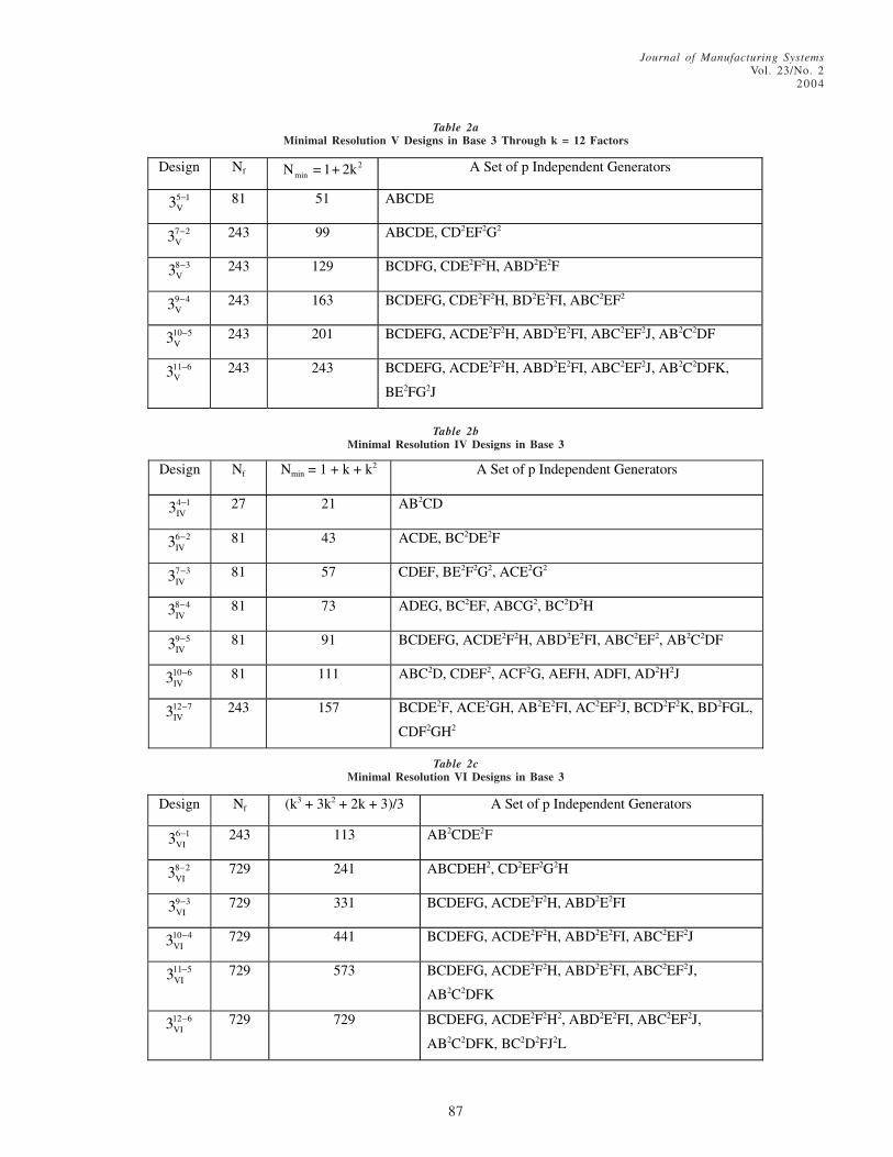
For base-3 designs, the sufficient number of runsfor a resolution III design is Nmin = 1 + 2k, but the 1 +2k distinct rows are generally smaller than Nf = 3k–p
rows of an orthogonal array and hence 1 + 2k mustbe rounded up to the next higher integer in powersof 3 (although the experimenter can leave some col-umns of a 3k–p OA empty and use them as residualsor simply unused). The minimum required numberof runs for a resolution V design in base 3 is givenby Nmin = 1 + 2k + 4(kC2) = 1 + 2k2 (only for k � 5),and again the value of 1 + 2k2 (if not already in pow-
ers of 3) has to be rounded up to the next higher inte-ger that can be expressed in powers of 3. Table 2asummarizes minimal resolution V designs through k= 12 factors in base 3. Note that Margolin (1969) doesnot provide sufficient run requirements for a base-3resolution R = V designs, but Conner and Zelen (1959)provide the independent generators for a few of the3R
k p− FFDs through k = 10, which are 37 2V
− , 39 4V
− , 310 5V
− ,36 2
IV− , 37 3
IV− , 38 4
IV− , 36 1
VI− , 39 3
VI− , and 39 5
IV− .
For base-3 designs, the sufficient required num-ber of runs for a minimal resolution IV design is Nf
Table 1bMinimal Resolution IV Designs in Base 2 Through k = 20 Factors
Design Nf k(k 3)1
4
++ A Set of p Independent Generators
6 2IV2 − 16 14.5 ABCE, BCDF
7 3IV2 − 16 18.5 ABCE, BCDF, ACDG
8 4IV2 − 16 23 ABCE, ABDF, BCDG, ACDH
9 4IV2 − 32 28 ABCF, BCDG, CDEH, ABDI
10 5IV2 − 32 33.5 ABCF, ABDG, ABEH, BCDI, BCEJ
11 6IV2 − 32 39.5 ABCF, ABDG, ABEH, BCDI, BCEJ, CDEK
12 7IV2 − 32 46 ABCF, ABDG, ABEH, BCDI, BCEJ, CDEK, ABCDEL
13 8IV2 − 32 53 ABCF, ABDG, ABEH, ACDI, ACEJ, ADEK, BCDL, BCEM
14 9IV2 − 32 60.5 ABCF, ABDG, ABEH, ACDI, ACEJ, ADEK, BCDL, BCEM,
CDEN
15 10IV2 − 32 68.5 ABCF, ABDG, ABEH, ACDI, ACEJ, ADEK, BCDL, BCEM,
BDEN, CDEO
16 11IV2 − 32 77 ABCF, ABDG, ABEH, ACDI, ACEJ, ADEK, BCDL, BCEM,
BDEN, CDEO, ABCDEP
17 11IV2 − 64 86 ABCFG, ABDFH, ABEFI, ACDFJ, ACEFK, ADEFL, BCDFM,
BCEFN, BDEFO, CDEP, ABCDEQ
18 12IV2 − 64 95.5 ABFG, ACFH, ADFI, AEFJ, BCFK, BDFL, BEFM, CDFN,
CEFO, DEFP, ABCQ, CDER
19 13IV2 − 64 105.5 ABFG, ACFH, ADFI, AEFJ, BCFK, BDFL, BEFM, CDFN,
CDEO, DEFP, ABCQ, ABDR, ABES
20 14IV2 − 64 116 ABHT, ABGS, ABFR, ABEQ, ABDP, ABCO, BFLM, CJKN,
DJLN, EKLN, FJKL, GJMN, HKMN, ILMN

Journal of Manufacturing SystemsVol. 23/No. 22004
86
> 1 + 2k + 1
2 [4 × kC2] = 1 + k + k2 for k � 4. Table 2b
summarizes resolution IV designs for base 3. Thereader should observe that our sufficient run require-ments for base-3 resolution IV designs (k � 4) areconsistent with that of Margolin’s (1969) Theorem 2requirement for minimum needed number of runs,which he lists as 3(2k – 1) because k2 + k + 1 > 3(2k– 1) for all k > 4. In a similar manner, the minimumand sufficient number of runs for a resolution VIdesign in base 3 is 1 + 2k + 4(kC2) +
1
2 [4(kC3)] = (k3
+ 3k2 + 2k + 3)/3. Table 2c summarizes resolution VIdesigns for base 3.
The above summary completes our review of clas-sical FFDs. Before relating some of Taguchi’s OAsto the classical FFDs, an example will be presentedto illustrate how to compute the sum of squares (SS)of any effect for balanced orthogonal factorial de-signs in base b (most commonly b = 2, 3, and 5).The concept of orthogonality and balance will be-come clearer at the end of the example.
Consider a 33 factorial with n = 2 observationsper FLC, where all the N = n × Nf = 2 × 27 = 54observations are taken in a completely random or-der. The qualitative factor A represents a type of drum(type 0, 1, 2), factor B represents the speed differen-tial between the conveyer belts for the liner/ply andthe drum (B0 = 5%, B1 = 7.5%, and B2 = 10%), andfactor C represents the concentricity of the bead withrespect to the drum (0 = not concentric, 1 = fairlyconcentric, and 2 = very concentric). The responsevariable, y, is the radial force harmonic (RFH) of apassenger tire coded by subtracting 20 pounds fromall 54 observations. The coding was done just to sim-plify computations and will not affect any of thecorrected SS in the analysis of variance (ANOVA)table. Table 3 lists the data.
The arbitrary columns of the OA for Table 3 areobtained by writing three (the exponent of b) col-umns of 0’s, 1’s, and 2’s arbitrarily, i.e., the first col-umn will be nine 0’s, nine 1’s, followed by nine 2’s.
Table 1cMinimal Resolution VI Designs in Base 2 Through k = 20 Factors
Design Nf (k3 + 3k2 + 8k + 12)/12 A Set of p Independent Generators
9 2VI2 − 128 88 ABCDFH, BCEFGI
10 2VI2 − 256 116 ABCFGH, CDEHIJ
11 3VI2 − 256 149.5 ABCDFI, BCDEGJ, ACDEHK
12 4VI2 − 256 189 ABCDEI, ABCFGJ, ABDFHK, ACEGHL
14 5VI2 − 512 288 ABCDEJ, ABCFGK, ABCHIL, ABDFHM, ABEGIN
15 6VI2 − 512 348.5 ABCDEJ, ABCFGK, ABCHIL, ABDFHM, ABEGIN,
ADEFIO
16 7VI2 − 512 417 ABCDEJ, ABCFGK, ABDFHL, ABEGIM, ADEFIN,
AEFGHO, ABCEFHIP
17 8VI2 − 512 494 ABCDEJ, ABCFGK, ABCHIL, ABDFHM, ABEGIN,
ADEFIO, BDGHIP, ACDEFGHQ
18 9VI2 − 512 580 ABCDEJ, ABCFGK, ABCHIL, ABDFHM, ABEGIN,
ADEFIO, BDGHIP, ACDEFGHQ, BCEFGHIR
19 9VI2 − 1024 675.5 ABCGHK, ABDGIL, ABEGJM, BEFHIN, ACDHJO,
ACEIJP, CFGHIQ, DEGHJR, DFHIJS
20 10VI2 − 1024 781 ABCDEK, ABCFGL, ABDFHM, ACDFIN, AEGHIO,
ABEFJP, BCGIJQ, BCDFGHJR, BEFGHS, CDEGIT
Journal of Manufacturing SystemsVol. 23/No. 2
2004
87
Table 2aMinimal Resolution V Designs in Base 3 Through k = 12 Factors
Table 2bMinimal Resolution IV Designs in Base 3
Table 2cMinimal Resolution VI Designs in Base 3
Design Nf 2
minN = 1+ 2k A Set of p Independent Generators
5 1V3 − 81 51 ABCDE
7 2V3 − 243 99 ABCDE, CD2EF2G2
8 3V3 − 243 129 BCDFG, CDE2F2H, ABD2E2F
9 4V3 − 243 163 BCDEFG, CDE2F2H, BD2E2FI, ABC2EF2
10 5V3 − 243 201 BCDEFG, ACDE2F2H, ABD2E2FI, ABC2EF2J, AB2C2DF
11 6V3 − 243 243 BCDEFG, ACDE2F2H, ABD2E2FI, ABC2EF2J, AB2C2DFK,
BE2FG2J
Design Nf Nmin = 1 + k + k2 A Set of p Independent Generators
4 1IV3 − 27 21 AB2CD
6 2IV3 − 81 43 ACDE, BC2DE2F
7 3IV3 − 81 57 CDEF, BE2F2G2, ACE2G2
8 4IV3 − 81 73 ADEG, BC2EF, ABCG2, BC2D2H
9 5IV3 − 81 91 BCDEFG, ACDE2F2H, ABD2E2FI, ABC2EF2, AB2C2DF
10 6IV3 − 81 111 ABC2D, CDEF2, ACF2G, AEFH, ADFI, AD2H2J
12 7IV3 − 243 157 BCDE2F, ACE2GH, AB2E2FI, AC2EF2J, BCD2F2K, BD2FGL,
CDF2GH2
Design Nf (k3 + 3k2 + 2k + 3)/3 A Set of p Independent Generators
6 1VI3 − 243 113 AB2CDE2F
8 2VI3 − 729 241 ABCDEH2, CD2EF2G2H
9 3VI3 − 729 331 BCDEFG, ACDE2F2H, ABD2E2FI
10 4VI3 − 729 441 BCDEFG, ACDE2F2H, ABD2E2FI, ABC2EF2J
11 5VI3 − 729 573 BCDEFG, ACDE2F2H, ABD2E2FI, ABC2EF2J,
AB2C2DFK
12 6VI3 − 729 729 BCDEFG, ACDE2F2H2, ABD2E2FI, ABC2EF2J,
AB2C2DFK, BC2D2FJ2L

Journal of Manufacturing SystemsVol. 23/No. 22004
88
The second column will consist of three 0’s, three1’s, three 2’s, and repeated twice more. The thirdcolumn will consist of 0, 1, and 2, but repeated eighttimes more to yield 27 rows. The total SS is obtainedby summing the square of all 54 observations (whichis called the uncorrected SS denoted by USS) andthen subtracting the correction factor CF = (y….)
2/54,
where 3 3 3 2
.... ijkri 1 j 1 k 1 r 1
y y= = = =
= ∑∑ ∑ ∑ , and Taguchi uses the un-
common notation Sm for the correction factor; notethat the index i extends over the factor A levels, jrefers to factor B levels, k extends over factor C lev-els, and r = 1, 2 implies that there are two repeatobservations (or replications) within each cell. Forexample, the cell (or FLC) 201 contains the responsesy3121 = 3.2 and y3122 = 5.5 so that y312. = 8.7, etc. Theuncorrected SS for Table 3 data is given by USS =
3 3 3 22ijkr
i 1 j 1 k 1 r 1y
= = = =∑∑ ∑ ∑ = 4.82 + 6.92 + … + 5.82 = 1850.40. The
reader should be cognizant of the fact that in devel-oping an ANOVA, each time that a real number issquared one degree of freedom is generated. Fur-ther, because degrees of freedom are additive (theorigin of these concepts lies in the assumption ofnormality for yijkr and the resulting noncentral chi-square distribution), then the USS for Table 3 willhave N = 2 × 33 = 54 df because there are n = 54normally distributed random numbers that are being
squared and added. The CF = 2139.2
358.8266654
= ,
which has only one degree of freedom because onlyone Gaussian number is being squared. Thus, thecorrected SS is given by CSS = SS(Total) = USS –
CF = 1850.40 – 358.82667 = 1491.57333 , whichhas 54 – 1 = 53 df.
Another reason that the CSS = ( )3 3 3 2 2
ijkr ....i 1 j 1 k 1 r 1
y y= = = =∑∑ ∑ ∑ −
has 53 df (instead of 54) is the fact that the 54squared terms in this last CSS have one constraint
among them, namely ( )3 3 3 2
ijkr ....i 1 j 1 k 1 r 1
y y 0= = = =∑∑ ∑ ∑ − ≡ . In all
factorial (or FF) designs, the Total SS decomposes intotwo orthogonal components, namely Model SS andResidual SS, i.e., SS(Total) = SS(Model) +SS(Residuals). For the data of Table 3, the source ofResiduals is from pure experimental error that is gen-erated from the variation within each of the 27 cells.If repeat observations are not made in at least oneFLC, then pure experimental error cannot be retrieved,and unless the design provides leftover degrees offreedom for residuals, no exact statistical test of sig-nificance can be made. For example, the FLC 000has two responses, 4.8 and 6.9, which contribute 4.82
+ 6.92 – ( )24.8 6.9
2
+ = 4.82 + 6.92 – 11.72/2 = 2.2050
to the overall pure error SS [denoted as SSPE orSS(PE)], and recalling the premise that every realnumber squared generates one degree of freedom,then the SSPE from the cell 000 carries a net of 1 + 1– 1 = 1 degree of freedom.
Similarly, the cell 202 has two responses, –2.1
and 3.1, which contribute (–2.1)2 + 3.12 – ( )2–2.1 3.1
2
+
= 13.52 (with one degree of freedom) to the overallSSPE. Because the above factorial design has 3 × 3 ×3 = 27 distinct FLCs and each cell contributes one
Table 3Data for the 33 Complete Factorial Example
Factor B B at level “0” → B at 5%
B1 → B at 7.5% B2 → B at 10%
C
A
C0 C1 C2 C0 C1 C2 C0 C1 C2 yi…
Type 0 4.8 1.0 –9.1
6.9 –2.1 –6.8
2.2 –1.1 –3.4
4.7 –5.6 2.1
10.3 6.8 3.5
9.2 4.2 7.2
34.8
Type 1 3.2 1.3 1.5
5.7 0.0 –3.2
2.7 –2.1 –10.1
6.9 –3.5 –7.7
8.3 3.4 1.3
9.2 5.2 2.9
25.0
Type 2 8.6 3.2 –2.1
7.7 5.5 3.1
8.6 4.1 –6.8
5.8 2.3 –4.2
11.2 7.6 6.6
10.7 1.7 5.8
79.4
y.jk. 36.9 8.9 –16.6 30.9 –5.9 –30.1 58.9 28.9 27.3 y…. = 139.2

Journal of Manufacturing SystemsVol. 23/No. 2
2004
89
degree of freedom to the overall pure error, SSPE musthave 27 df. Adding the 27 one-degree-of-freedomSS yields SS(PE) = 2.2050 + 4.8050 + 2.6450 +3.1250 + 10.1250 + 15.1250 + 0.6050 + 3.3800 +6.8450 + 3.1250 + 0.8450 + 11.0450 + 8.8200 +0.9800 + 2.8800 + 0.4050 + 1.6200 + 1.2800 +0.4050 + 2.6450 + 13.5200 + 3.9200 + 1.6200 +3.3800 + 0.1250 + 17.4050 + 0.3200 = 123.2000.
Because the above factorial design has a total of53 df, due to orthogonality the Model SS must have53 – 27 = 26 df. Clearly, one way to obtain theSS(Model) is by subtracting SS(PE) from SS(Total),i.e., SS(Model) = SS(Total, with 53 df) – SS(PE, with27 df ) = 1491.57333 – 123.20 = 1368.37333 (with26 df). The above method of computing the SS(PE)and SS(Model) is at best time-consuming and cum-bersome. Because pure experimental error originatesfrom the internal variation within the same cell, varia-tion due to the model must originate from the factthat cell averages are different. In short, the Model SSmust come from variability among distinct FLCs. Fur-ther, because n = 2 for all 27 cells, then we may aswell compare cell subtotals directly (instead of theiraverages) to assess the contribution of model terms tothe SS(Total). If we remove the internal variationwithin all cells from Table 3, the resulting Table 4 willdepict the variations among (or between) the 27 cells.
Another pattern that will prevail in computingany SS in all orthogonally balanced factorial de-signs is the fact that every squared term has a spe-cific divisor. The divisor is always the number ofindividual observations that comprise the squaredterm. The formula for the correction factor is CF =(grand sum of all observations)2/divisor. To determine
what the value of the divisor is, the question to ask ishow many individual observations have to be addedto obtain y…. = “grand sum of all observations.” Theanswer is N = 54, and hence this divisor has to be 54,i.e., CF = (y….)
2/54. As yet another example, if wewish to square the subtotal for level zero of A, de-noted by A0, then the required divisor for 2
0A = (34.8)2
(see Table 3) has to be 18 because 18 individual ob-servations have to be added to obtain A0 = 34.8.
Having established some rules for SS computa-tions, we are now in a position to compute the over-all Model SS as follows. Recall that the modeldescribes the variation among different distinct FLCs,of which there are 27. Thus, we have to square the27 terms in Table 4 but divide by 2 because everyterm in Table 4 was obtained from adding two indi-vidual responses. However, such an USS will have27 df (this is due to the fact that a single Gaussianterm squared generates exactly 1 df, the origin ofwhich lies in the noncentral chi-squared (�2) distri-bution) and we have already argued that the modelfor the above experiment must have 26 df becausethe 27 squared terms in SS(Model) =
( )3 3 3 2
ijk. ....i 1 j 1 k 1
2 y y= = =∑∑ ∑ − have one constraint
( )3 3 3 2
ijk. ....i 1 j 1 k 1 r 1
y y 0= = = =∑∑ ∑ ∑ − ≡ among them; thus, we have to
correct by subtracting the CF, i.e.,
( )( ) ( )
( )
2 22 2 2
2
SS Model
11.7 1.1 15.9 ... 9.3 12.4
2
345.4 139.20CF 1368.37333 with 26 df
2 54
=
+ − + − + + +−
= − =
Table 4Depicting Variability Among (or Between) the 27 Cells
Factor B B at level “0” → B at 5%
B at 1 → 7.5% B at 2 →10%
C
A
C0 1 2 0 C at 1 2 0 1 C at 2 yi…
Type 0 11.7 –1.1 –15.9 6.9 –6.7 –1.3 19.5 11.0 10.7 34.8
Type 1 8.9 1.3 –1.7 9.6 –5.6 –17.8 17.5 8.6 4.2 25.0
Type 2 16.3 8.7 1.0 14.4 6.4 –11.0 21.9 9.3 12.4 79.4
y.jk. 36.9 8.9 –16.6 30.9 –5.9 –30.1 58.9 28.9 27.3 y…. = 139.2
Journal of Manufacturing SystemsVol. 23/No. 22004
90
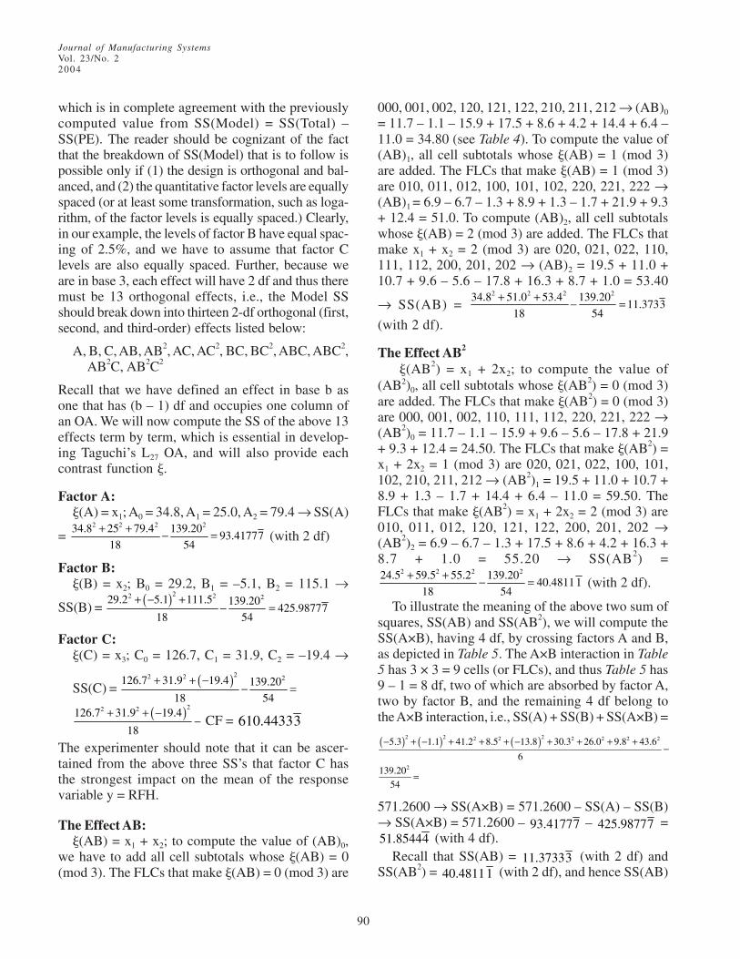
which is in complete agreement with the previouslycomputed value from SS(Model) = SS(Total) –SS(PE). The reader should be cognizant of the factthat the breakdown of SS(Model) that is to follow ispossible only if (1) the design is orthogonal and bal-anced, and (2) the quantitative factor levels are equallyspaced (or at least some transformation, such as loga-rithm, of the factor levels is equally spaced.) Clearly,in our example, the levels of factor B have equal spac-ing of 2.5%, and we have to assume that factor Clevels are also equally spaced. Further, because weare in base 3, each effect will have 2 df and thus theremust be 13 orthogonal effects, i.e., the Model SSshould break down into thirteen 2-df orthogonal (first,second, and third-order) effects listed below:
A, B, C, AB, AB2, AC, AC2, BC, BC2, ABC, ABC2,AB2C, AB2C2
Recall that we have defined an effect in base b asone that has (b – 1) df and occupies one column ofan OA. We will now compute the SS of the above 13effects term by term, which is essential in develop-ing Taguchi’s L27 OA, and will also provide eachcontrast function �.
Factor A:�(A) = x1; A0 = 34.8, A1 = 25.0, A2 = 79.4 Æ SS(A)
= 2 2 2 234.8 25 79.4 139.20
93.4177718 54
+ + − = (with 2 df)
Factor B:�(B) = x2; B0 = 29.2, B1 = –5.1, B2 = 115.1 Æ
SS(B) = ( )22 2 229.2 5.1 111.5 139.20425.98777
18 54
+ − +− =
Factor C:�(C) = x3; C0 = 126.7, C1 = 31.9, C2 = –19.4 Æ
SS(C) = ( )22 2 2126.7 31.9 19.4 139.20
18 54
+ + −− =
( )22 2126.7 31.9 19.4
18
+ + −− CF = 610.44333
The experimenter should note that it can be ascer-tained from the above three SS’s that factor C hasthe strongest impact on the mean of the responsevariable y = RFH.
The Effect AB:�(AB) = x1 + x2; to compute the value of (AB)0,
we have to add all cell subtotals whose �(AB) = 0(mod 3). The FLCs that make �(AB) = 0 (mod 3) are
000, 001, 002, 120, 121, 122, 210, 211, 212 Æ (AB)0
= 11.7 – 1.1 – 15.9 + 17.5 + 8.6 + 4.2 + 14.4 + 6.4 –11.0 = 34.80 (see Table 4). To compute the value of(AB)1, all cell subtotals whose �(AB) = 1 (mod 3)are added. The FLCs that make �(AB) = 1 (mod 3)are 010, 011, 012, 100, 101, 102, 220, 221, 222 Æ(AB)1 = 6.9 – 6.7 – 1.3 + 8.9 + 1.3 – 1.7 + 21.9 + 9.3+ 12.4 = 51.0. To compute (AB)2, all cell subtotalswhose �(AB) = 2 (mod 3) are added. The FLCs thatmake x1 + x2 = 2 (mod 3) are 020, 021, 022, 110,111, 112, 200, 201, 202 Æ (AB)2 = 19.5 + 11.0 +10.7 + 9.6 – 5.6 – 17.8 + 16.3 + 8.7 + 1.0 = 53.40
Æ SS(AB) = 2 2 2 234.8 51.0 53.4 139.20
11.373318 54
+ + − =
(with 2 df).
The Effect AB2
�(AB2) = x1 + 2x2; to compute the value of(AB2)0, all cell subtotals whose �(AB2) = 0 (mod 3)are added. The FLCs that make �(AB2) = 0 (mod 3)are 000, 001, 002, 110, 111, 112, 220, 221, 222 →(AB2)0 = 11.7 – 1.1 – 15.9 + 9.6 – 5.6 – 17.8 + 21.9+ 9.3 + 12.4 = 24.50. The FLCs that make �(AB2) =x1 + 2x2 = 1 (mod 3) are 020, 021, 022, 100, 101,102, 210, 211, 212 → (AB2)1 = 19.5 + 11.0 + 10.7 +8.9 + 1.3 – 1.7 + 14.4 + 6.4 – 11.0 = 59.50. TheFLCs that make �(AB2) = x1 + 2x2 = 2 (mod 3) are010, 011, 012, 120, 121, 122, 200, 201, 202 →(AB2)2 = 6.9 – 6.7 – 1.3 + 17.5 + 8.6 + 4.2 + 16.3 +8.7 + 1.0 = 55.20 → SS(AB2) =
2 2 2 224.5 59.5 55.2 139.2040.48111
18 54
+ + − = (with 2 df).
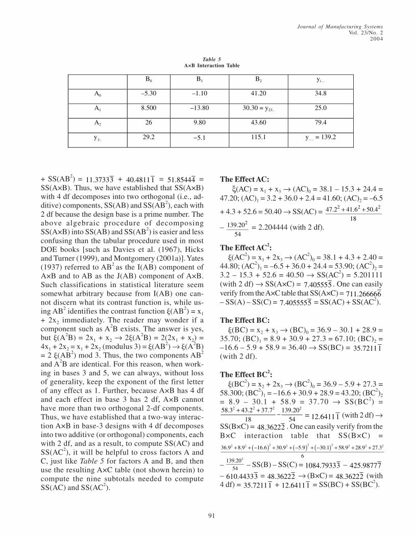
To illustrate the meaning of the above two sum ofsquares, SS(AB) and SS(AB2), we will compute theSS(A×B), having 4 df, by crossing factors A and B,as depicted in Table 5. The A×B interaction in Table5 has 3 × 3 = 9 cells (or FLCs), and thus Table 5 has9 – 1 = 8 df, two of which are absorbed by factor A,two by factor B, and the remaining 4 df belong tothe A×B interaction, i.e., SS(A) + SS(B) + SS(A×B) =
( ) ( ) ( )2 2 22 2 2 2 2 2
2
5.3 1.1 41.2 8.5 13.8 30.3 26.0 9.8 43.6
6
139.20
54
− + − + + + − + + + +−
=
571.2600 Æ SS(A×B) = 571.2600 – SS(A) – SS(B)Æ SS(A×B) = 571.2600 – 93.41777 – 425.98777 =51.85444 (with 4 df).
Recall that SS(AB) = 11.37333 (with 2 df) andSS(AB2) = 40.48111 (with 2 df), and hence SS(AB)
Journal of Manufacturing SystemsVol. 23/No. 2
2004
91
+ SS(AB2) = 11.37333 + 40.48111 = 51.85444 =SS(A×B). Thus, we have established that SS(A×B)with 4 df decomposes into two orthogonal (i.e., ad-ditive) components, SS(AB) and SS(AB2), each with2 df because the design base is a prime number. Theabove algebraic procedure of decomposingSS(A×B) into SS(AB) and SS(AB2) is easier and lessconfusing than the tabular procedure used in mostDOE books [such as Davies et al. (1967), Hicksand Turner (1999), and Montgomery (2001a)]. Yates(1937) referred to AB2 as the I(AB) component ofA×B and to AB as the J(AB) component of A×B.Such classifications in statistical literature seemsomewhat arbitrary because from I(AB) one can-not discern what its contrast function is, while us-ing AB2 identifies the contrast function �(AB2) = x1
+ 2x2 immediately. The reader may wonder if acomponent such as A2B exists. The answer is yes,but �(A2B) = 2x1 + x2 Æ 2�(A2B) = 2(2x1 + x2) =4x1 + 2x2 = x1 + 2x2 (modulus 3) = �(AB2) Æ �(A2B)= 2 �(AB2) mod 3. Thus, the two components AB2
and A2B are identical. For this reason, when work-ing in bases 3 and 5, we can always, without lossof generality, keep the exponent of the first letterof any effect as 1. Further, because A×B has 4 dfand each effect in base 3 has 2 df, A×B cannothave more than two orthogonal 2-df components.Thus, we have established that a two-way interac-tion A×B in base-3 designs with 4 df decomposesinto two additive (or orthogonal) components, eachwith 2 df, and as a result, to compute SS(AC) andSS(AC2), it will be helpful to cross factors A andC, just like Table 5 for factors A and B, and thenuse the resulting A×C table (not shown herein) tocompute the nine subtotals needed to computeSS(AC) and SS(AC2).
The Effect AC:ξ(AC) = x1 + x3 → (AC)0 = 38.1 – 15.3 + 24.4 =
47.20; (AC)1 = 3.2 + 36.0 + 2.4 = 41.60; (AC)2 = –6.5
+ 4.3 + 52.6 = 50.40 → SS(AC) = 2 2 247.2 41.6 50.4
18
+ +
– 2139.20
54 = 2.204444 (with 2 df).
The Effect AC2:�(AC2) = x1 + 2x3 Æ (AC2)0 = 38.1 + 4.3 + 2.40 =
44.80; (AC2)1 = –6.5 + 36.0 + 24.4 = 53.90; (AC2)2 =3.2 – 15.3 + 52.6 = 40.50 Æ SS(AC2) = 5.201111(with 2 df) Æ SS(A×C) = 7.405555 . One can easilyverify from the A×C table that SS(A×C) = 711.266666– SS(A) – SS(C) = 7.4055555 = SS(AC) + SS(AC2).
The Effect BC:�(BC) = x2 + x3 Æ (BC)0 = 36.9 – 30.1 + 28.9 =
35.70; (BC)1 = 8.9 + 30.9 + 27.3 = 67.10; (BC)2 =–16.6 – 5.9 + 58.9 = 36.40 Æ SS(BC) = 35.72111(with 2 df).
The Effect BC2:�(BC2) = x2 + 2x3 Æ (BC2)0 = 36.9 – 5.9 + 27.3 =
58.300; (BC2)1 = –16.6 + 30.9 + 28.9 = 43.20; (BC2)2
= 8.9 – 30.1 + 58.9 = 37.70 Æ SS(BC2) =2 2 2 258.3 43.2 37.7 139.20
18 54
+ + − = 12.64111 (with 2 df) ÆSS(B×C) = 48.36222 . One can easily verify from theB×C interaction table that SS(B×C) =
( ) ( ) ( )2 2 22 2 2 2 2 236.9 8.9 16.6 30.9 5.9 30.1 58.9 28.9 27.3
6
+ + − + + − + − + + +
– 2139.20
54 – SS(B) – SS(C) = 1084.79333 – 425.98777
– 610.44333 = 48.36222 Æ (B×C) = 48.36222 (with4 df) = 35.72111 + 12.64111 = SS(BC) + SS(BC2).
Table 5A×B Interaction Table
B0 B1 B2 yi…
A0 –5.30 –1.10 41.20 34.8
A1 8.500 –13.80 30.30 = y23.. 25.0
A2 26 9.80 43.60 79.4
y.j.. 29.2 −5.1 115.1 y…. = 139.2

Journal of Manufacturing SystemsVol. 23/No. 22004
92
The Effect ABC:�(ABC) = x1 + x2 + x3 Æ From Table 4, the value
of (ABC)0 is computed using the nine FLCs (000,012, 021, 102, 120, 111, 201, 210, 222) that makethe contrast function �(ABC) = x1 + x2 + x3 = 0 (mod3). Thus, (ABC)0 = 11.7 – 1.3 + 11.0 – 1.7 + 17.5 –5.6 + 8.7 + 14.4 + 12.4 = 67.10; (ABC)1 = –1.1 + 6.9+ 10.7 + 8.9 – 17.8 + 8.6 + 1.0 + 6.4 + 21.9 = 45.50;(ABC)2 = –15.9 – 6.7 + 19.5 + 1.3 + 9.6 + 4.2 + 16.3
– 11.0 + 9.3 = 26.60 Æ SS(ABC) = 2 2 267.1 45.5 26.6
18
+ +
– 2139.20
54 = 45.630 (with 2 df).
The Effect ABC2:�(ABC2) = x1 + x2 + 2x3 → From Table 4, the value
of (ABC2)0 is computed using the nine FLCs thatmake the contrast function �(ABC2) = x1 + x2 + 2x3 =0 (mod 3). The nine FLCs that make the contrastfunction �(ABC2) = x1 + x2 + 2x3 = 1 are 002, 021,010, 100, 111, 122, 220, 212, 201. Thus, (ABC2)0 =11.7 – 6.7 + 10.7 + 1.3 – 17.8 + 17.5 + 1.0 + 14.4 +9.3 = 41.40; (ABC2)1 = –15.9 + 11.0 + 6.9 + 8.9 –5.6 + 4.2 + 21.9 – 11 + 8.7 = 29.10; similarly, (ABC2)2
= –1.1 – 1.3 + 19.5 – 1.7 + 9.6 + 8.6 + 16.3 + 6.4 +
12.4 = 68.70 Æ SS(ABC2) = 2 2 241.4 29.1 68.7
18
+ + –
2139.20
54 = 45.64333 (with 2 df).
The Effect AB2C:�(AB2C) = x1 + 2x2 + x3 → From Table 4, the value
of (AB2C)0 is computed using the nine FLCs thatmake the contrast function �(AB2C) = x1 + 2x2 + x3 =0 (mod 3). Thus, (AB2C)0 = 11.7 – 6.7 + 10.7 – 1.7+ 9.6 + 8.6 + 8.7 – 11.0 + 21.9 = 51.80; (AB2C)1 =–1.1 – 1.3 + 19.5 + 8.9 – 5.6 + 4.2 + 1.0 + 14.4 +9.3 = 49.30; (AB2C)2 = –15.9 + 6.9 + 11.0 + 1.3 –17.8 + 17.5 + 16.3 + 6.4 + 12.4 = 38.10 → SS(AB2C)
= 2 2 251.8 49.3 38.1
18
+ + –
2139.20
54 = 5.91444 (with 2 df).
The Effect AB2C2:�(AB2C2) = x1 + 2x2 + 2x3 → From Table 4, the
value of (AB2C2)0 is computed using the nine FLCsthat make the contrast function �(AB2C2) = x1 + 2x2
+ 2x3 = 0 (mod 3). Thus, (AB2C2)0 = 11.7 – 1.3 +11.0 + 1.3 + 9.6 + 4.2 + 1.0 + 6.4 + 21.9 = 65.80;(AB2C2)1 = –15.9 – 6.7 + 19.5 + 8.9 – 17.8 + 8.6 +8.7 + 14.4 + 12.4 = 32.10; (AB2C2)2 = –1.1 + 6.9 +10.7 – 1.7 – 5.6 + 17.5 + 16.3 – 11.0 + 9.3 = 41.30
→ SS(AB2C2) = 2 2 265.8 32.1 41.3
18
+ + –
2139.20
54 =
33.71444 (with 2 df).
The above base-3 algebraic procedure using thecontrast function to compute the four orthogonalcomponents of the second-order (or three-way) in-teraction A×B×C (with 8 df) is straightforward andleaves no room for confusion and/or error. However,the tabular procedure that has been used in statisti-cal literature in the past 50 years can lead to confu-sion and misclassification of the four orthogonalcomponents SS(ABC), SS(ABC2), SS(AB2C), andSS(AB2C2) of SS(A×B×C). For example, due to theuse of tabular procedure the two componentsSS(ABC2) and SS(ABC) atop p. 372 of Montgom-ery (2001a) are reversed (albeit a minormisclassification) because the value of SS(ABC2) is584.11 (not 18.77 as reported) and the value ofSS(ABC) is 18.77. Similarly, the two componentsSS(DOC) and SS(DOC2) near the bottom of p. 286of Hicks and Turner (1999) are also reversed. Thevalue of SS(DOC) to two decimals is 0.30 (not 0.19as reported) and the correct value of SS(DOC2) is 0.19.
The last 13 SS computations verify the fact thatSS(Model) = 1368.37333 (with 26 df) decomposesinto 13 orthogonal components, A, B, C, AB, AB2,AC, AC2, BC, BC2, ABC, ABC2, AB2C, and AB2C2.By orthogonal breakdown of SS(Model) is meantthat SS(Model) = SS(A) + SS(B) + SS(C) + SS(AB) +SS(AB2) + SS(AC) + SS(AC2) + SS(BC) + SS(BC2) +SS(ABC) + SS(ABC2) + SS(AB2C) + SS(AB2C2) =1368.37333 .
It is paramount to note that if a complete factorialdesign of any base b is orthogonal and balanced,then the SS(Model) always decomposes into the SSof main factors and the SS of interactions of all pos-sible orders. For example, a complete orthogonal 43
factorial design with the same number of observa-tions, n � 1, per FLC possesses the orthogonal de-composition of SS(Model) = SS(A) + SS(B) + SS(C)+ SS(A×B) + SS(A×C) + SS(B×C) + SS(A×B×C).However, because the design base b = 4 is not aprime number, the orthogonal decomposition ofSS(A×B) with 9 df into SS(AB), SS(AB2), andSS(AB3) [or into SS(A2B3), SS(A3B2), and SS(A2B2)]each with 3 df does not exist. We have verified thatthe three components SS(AB), SS(AB2), andSS(A3B2) are orthogonal in some 42 designs, but thesethree components are not orthogonal to factors A
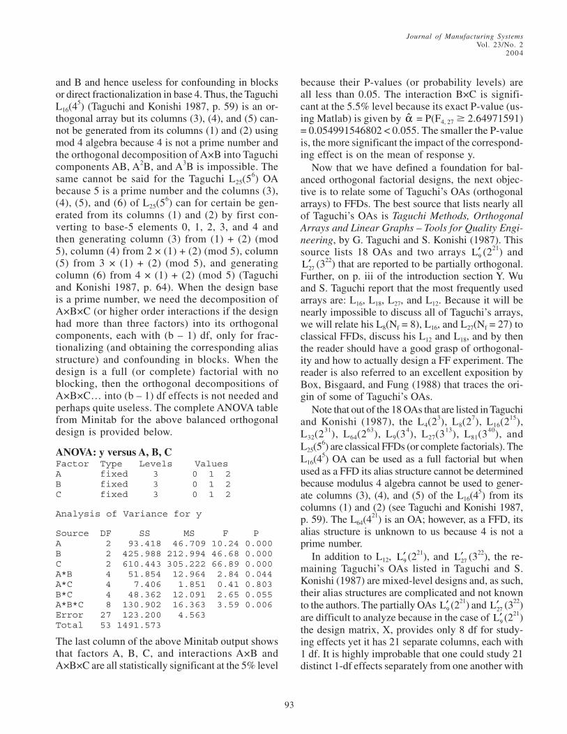
Journal of Manufacturing SystemsVol. 23/No. 2
2004
93
and B and hence useless for confounding in blocksor direct fractionalization in base 4. Thus, the TaguchiL16(4
5) (Taguchi and Konishi 1987, p. 59) is an or-thogonal array but its columns (3), (4), and (5) can-not be generated from its columns (1) and (2) usingmod 4 algebra because 4 is not a prime number andthe orthogonal decomposition of A×B into Taguchicomponents AB, A2B, and A3B is impossible. Thesame cannot be said for the Taguchi L25(5
6) OAbecause 5 is a prime number and the columns (3),(4), (5), and (6) of L25(5
6) can for certain be gen-erated from its columns (1) and (2) by first con-verting to base-5 elements 0, 1, 2, 3, and 4 andthen generating column (3) from (1) + (2) (mod5), column (4) from 2 × (1) + (2) (mod 5), column(5) from 3 × (1) + (2) (mod 5), and generatingcolumn (6) from 4 × (1) + (2) (mod 5) (Taguchiand Konishi 1987, p. 64). When the design baseis a prime number, we need the decomposition ofA×B×C (or higher order interactions if the designhad more than three factors) into its orthogonalcomponents, each with (b – 1) df, only for frac-tionalizing (and obtaining the corresponding aliasstructure) and confounding in blocks. When thedesign is a full (or complete) factorial with noblocking, then the orthogonal decompositions ofA×B×C… into (b – 1) df effects is not needed andperhaps quite useless. The complete ANOVA tablefrom Minitab for the above balanced orthogonaldesign is provided below.
ANOVA: y versus A, B, CFactor Type Levels ValuesA fixed 3 0 1 2B fixed 3 0 1 2C fixed 3 0 1 2
Analysis of Variance for y
Source DF SS MS F PA 2 93.418 46.709 10.24 0.000B 2 425.988 212.994 46.68 0.000C 2 610.443 305.222 66.89 0.000A*B 4 51.854 12.964 2.84 0.044A*C 4 7.406 1.851 0.41 0.803B*C 4 48.362 12.091 2.65 0.055A*B*C 8 130.902 16.363 3.59 0.006Error 27 123.200 4.563Total 53 1491.573
The last column of the above Minitab output showsthat factors A, B, C, and interactions A×B andA×B×C are all statistically significant at the 5% level
because their P-values (or probability levels) areall less than 0.05. The interaction B×C is signifi-cant at the 5.5% level because its exact P-value (us-ing Matlab) is given by α = P(F4, 27 � 2.64971591)= 0.054991546802 < 0.055. The smaller the P-valueis, the more significant the impact of the correspond-ing effect is on the mean of response y.
Now that we have defined a foundation for bal-anced orthogonal factorial designs, the next objec-tive is to relate some of Taguchi’s OAs (orthogonalarrays) to FFDs. The best source that lists nearly allof Taguchi’s OAs is Taguchi Methods, OrthogonalArrays and Linear Graphs – Tools for Quality Engi-neering, by G. Taguchi and S. Konishi (1987). Thissource lists 18 OAs and two arrays ′L9 (221) and
′L27 (322) that are reported to be partially orthogonal.Further, on p. iii of the introduction section Y. Wuand S. Taguchi report that the most frequently usedarrays are: L16, L18, L27, and L12. Because it will benearly impossible to discuss all of Taguchi’s arrays,we will relate his L8(Nf = 8), L16, and L27(Nf = 27) toclassical FFDs, discuss his L12 and L18, and by thenthe reader should have a good grasp of orthogonal-ity and how to actually design a FF experiment. Thereader is also referred to an excellent exposition byBox, Bisgaard, and Fung (1988) that traces the ori-gin of some of Taguchi’s OAs.
Note that out of the 18 OAs that are listed in Taguchiand Konishi (1987), the L4(2
3), L8(27), L16(2
15),L32(231), L64(263), L9(34), L27(313), L81(340), andL25(5
6) are classical FFDs (or complete factorials). TheL16(4
5) OA can be used as a full factorial but whenused as a FFD its alias structure cannot be determinedbecause modulus 4 algebra cannot be used to gener-ate columns (3), (4), and (5) of the L16(4
5) from itscolumns (1) and (2) (see Taguchi and Konishi 1987,p. 59). The L64(4
21) is an OA; however, as a FFD, itsalias structure is unknown to us because 4 is not aprime number.
In addition to L12, ′L9 (221), and ′L27 (322), the re-maining Taguchi’s OAs listed in Taguchi and S.Konishi (1987) are mixed-level designs and, as such,their alias structures are complicated and not knownto the authors. The partially OAs ′L9 (221) and ′L27 (322)are difficult to analyze because in the case of ′L9 (221)the design matrix, X, provides only 8 df for study-ing effects yet it has 21 separate columns, each with1 df. It is highly improbable that one could study 21distinct 1-df effects separately from one another with

Journal of Manufacturing SystemsVol. 23/No. 22004
94
nine runs that yield only 8 df. We ran Taguchi’s′L9 (221) on Minitab’s GLM and Minitab reported rank
deficiency and positive SS’s only for eight effects,as expected. The remaining 13 SS’s were reportedto have zero SS with zero df. Similarly, the ′L27 (322)partially orthogonal design matrix provides 26 dffor studying different 2-df effects, but it has 22 col-umns that need 44 df. Note that with a 26-df designmatrix in base 3 one can study a maximum of thir-teen 2-df effects without aliasing them. We would haveto recommend against the use of these last twoTaguchi’s partially orthogonal arrays.
6. Some Commonly Used Taguchi’s OAs(Taguchi L8(2
7) OA)The subscript 8 in L8(2
7) implies that the designmatrix has Nf = 8 distinct rows (or distinct FLCs)and thus provides 7 (= 8 – 1) df for studying sevenorthogonal effects, implying that the design matrixcan have a maximum of seven orthogonal columns.Further, because 8 = 23, exactly three arbitrary col-umns can be written, but the remaining four columnsmust be obtained from the three arbitrary columns.
We use a variation of the procedure first introducedby Kackar and Tsui (1990) by first displaying thethree arbitrary columns in Table 6 (using the base-2elements 0 for the low level, 1 for the high level, andlater on converting to Taguchi’s notation of 1 and 2),and then embedding a 23 full factorial into the L8
OA. The reader should bear in mind that for Taguchi’sOAs, we are using the notation that the numbers in-side the parentheses ( ) generally imply columns, thatis, (1) means column 1, (2) means column 2, and soon. To generate column 3, we simply add columns 1and 2 (modulus 2), that is, (3) = (1) + (2), mod 2. Togenerate (5), we add (1) and (4) mod 2, that is, (5) =(1) + (4), mod 2; similarly, (6) = (2) + (4), and (7) = (1)+ (2) + (4) mod 2. The entire design matrix using thisprocedure is provided in Table 7a. Note that in Table7a it will be totally impossible to generate anothercolumn (i.e., an eighth distinct column) that is orthogo-nal to the above seven columns because the matrixhas only 7 df and each column (because of two lev-els) carries exactly 1 df. To convert Table 7a toTaguchi’s format, we simply place the third arbitrarycolumn in column 4 and the interaction (1) + (2) col-umn in column 3 as shown in Table 7b.
Table 7b now shows that the interaction of col-umns 1 and 2 is column 3, that is, if factor A is as-
signed to (1) and B is assigned to column 2, thentheir interaction A×B must be assigned to (3) be-cause the contrast function of A×B interaction is�(AB) = x1 + x2 = (1) + (2), mod 2. Similarly, if factorC is assigned to (4), then AC interaction must beassigned to column (5) (if the experimenter desiresto study AC interaction). Further, the BC interactionmust be assigned to (6) because (2) + (4) = (6), mod2, and ABC interaction must be assigned to (7) be-cause (1) + (2) + (4) = (7), mod 2.
We next convert to Taguchi’s notation by trans-forming 0 → 1 and 1 → 2 as displayed in Table 7c.Table 7c is identical to the Taguchi’s OA on p. 1 ofTaguchi and Konishi (1987). So far, we have dis-cussed how to construct the Taguchi L8 OA for a full23 factorial. The next step is to construct the 24–1
FFD using Taguchi’s L8 OA. Here there are four fac-tors, A, B, C, and D, that will occupy four out of theseven columns. Although not necessary, it is usuallybest to assign the main factors to the three arbitrarycolumns, which are (1), (2), and (4). Because theFFD 24–1 has only p = 1 generator, it is best to maxi-mize resolution by selecting g = ABCD as the de-sign generator. This means that we should assignour factors to the columns of Taguchi’s L8 OA insuch a manner as to attain the alias structure A =BCD, B = ACD, C = ABD, D = ABC, AB = CD, AC =BD, and AD = BC. If our design matrix shows that D= ABC, then a resolution R = IV is guaranteed. Oneway to attain this maximum resolution is to assign Ato (1), B to (2), and C to (4), and because (1) + (2) +(4) = (7), mod 2, we must assign factor D to column(7); this assignment will ensure a resolution IV de-sign because both effects ABC and D will occupy
Table 6Three Arbitrary Columns of the Taguchi L8 OA in
Base-2 Notation
(1) (2) (4)
0
0
0
0
0
0
1
1
0
1
0
1
1
1
1
1
0
0
1
1
0
1
0
1
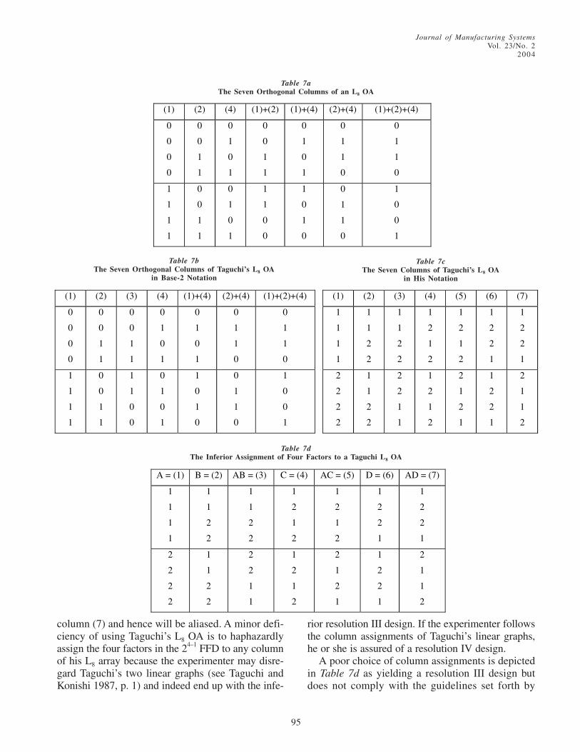
Journal of Manufacturing SystemsVol. 23/No. 2
2004
95
Table 7aThe Seven Orthogonal Columns of an L8 OA
(1) (2) (4) (1)+(2) (1)+(4) (2)+(4) (1)+(2)+(4)
0
0
0
0
0
0
1
1
0
1
0
1
0
0
1
1
0
1
0
1
0
1
1
0
0
1
1
0
1
1
1
1
0
0
1
1
0
1
0
1
1
1
0
0
1
0
1
0
0
1
1
0
1
0
0
1
Table 7b
The Seven Orthogonal Columns of Taguchi’s L8 OAin Base-2 Notation
(1) (2) (3) (4) (1)+(4) (2)+(4) (1)+(2)+(4)
0
0
0
0
0
0
1
1
0
0
1
1
0
1
0
1
0
1
0
1
0
1
1
0
0
1
1
0
1
1
1
1
0
0
1
1
1
1
0
0
0
1
0
1
1
0
1
0
0
1
1
0
1
0
0
1
Table 7cThe Seven Columns of Taguchi’s L8 OA
in His Notation
(1) (2) (3) (4) (5) (6) (7)
1
1
1
1
1
1
2
2
1
1
2
2
1
2
1
2
1
2
1
2
1
2
2
1
1
2
2
1
2
2
2
2
1
1
2
2
2
2
1
1
1
2
1
2
2
1
2
1
1
2
2
1
2
1
1
2
column (7) and hence will be aliased. A minor defi-ciency of using Taguchi’s L8 OA is to haphazardlyassign the four factors in the 24–1 FFD to any columnof his L8 array because the experimenter may disre-gard Taguchi’s two linear graphs (see Taguchi andKonishi 1987, p. 1) and indeed end up with the infe-
A = (1) B = (2) AB = (3) C = (4) AC = (5) D = (6) AD = (7)
1
1
1
1
1
1
2
2
1
1
2
2
1
2
1
2
1
2
1
2
1
2
2
1
1
2
2
1
2
2
2
2
1
1
2
2
2
2
1
1
1
2
1
2
2
1
2
1
1
2
2
1
2
1
1
2
Table 7dThe Inferior Assignment of Four Factors to a Taguchi L8 OA
rior resolution III design. If the experimenter followsthe column assignments of Taguchi’s linear graphs,he or she is assured of a resolution IV design.
A poor choice of column assignments is depictedin Table 7d as yielding a resolution III design butdoes not comply with the guidelines set forth by
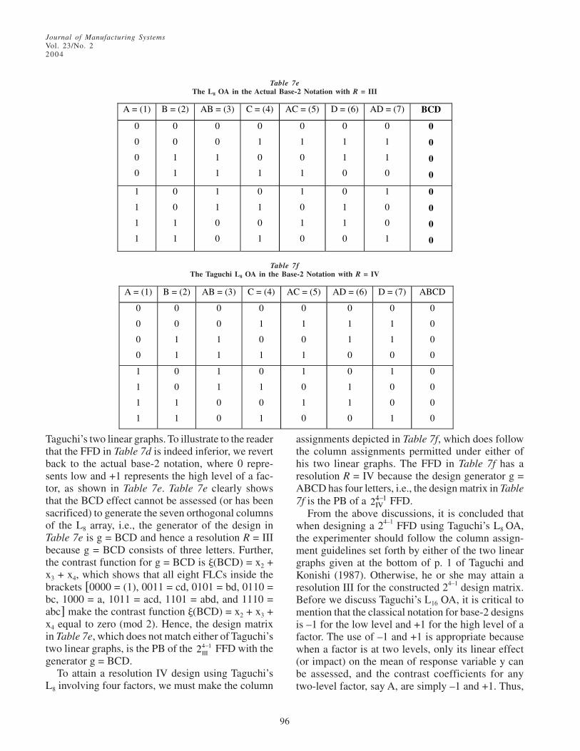
Journal of Manufacturing SystemsVol. 23/No. 22004
96
Taguchi’s two linear graphs. To illustrate to the readerthat the FFD in Table 7d is indeed inferior, we revertback to the actual base-2 notation, where 0 repre-sents low and +1 represents the high level of a fac-tor, as shown in Table 7e. Table 7e clearly showsthat the BCD effect cannot be assessed (or has beensacrificed) to generate the seven orthogonal columnsof the L8 array, i.e., the generator of the design inTable 7e is g = BCD and hence a resolution R = IIIbecause g = BCD consists of three letters. Further,the contrast function for g = BCD is �(BCD) = x2 +x3 + x4, which shows that all eight FLCs inside thebrackets [0000 = (1), 0011 = cd, 0101 = bd, 0110 =bc, 1000 = a, 1011 = acd, 1101 = abd, and 1110 =abc] make the contrast function �(BCD) = x2 + x3 +x4 equal to zero (mod 2). Hence, the design matrixin Table 7e, which does not match either of Taguchi’stwo linear graphs, is the PB of the 24 1
III− FFD with the
generator g = BCD.To attain a resolution IV design using Taguchi’s
L8 involving four factors, we must make the column
assignments depicted in Table 7f, which does followthe column assignments permitted under either ofhis two linear graphs. The FFD in Table 7f has aresolution R = IV because the design generator g =ABCD has four letters, i.e., the design matrix in Table7f is the PB of a 4 1
IV2 − FFD.From the above discussions, it is concluded that
when designing a 24–1 FFD using Taguchi’s L8 OA,the experimenter should follow the column assign-ment guidelines set forth by either of the two lineargraphs given at the bottom of p. 1 of Taguchi andKonishi (1987). Otherwise, he or she may attain aresolution III for the constructed 24–1 design matrix.Before we discuss Taguchi’s L16 OA, it is critical tomention that the classical notation for base-2 designsis –1 for the low level and +1 for the high level of afactor. The use of –1 and +1 is appropriate becausewhen a factor is at two levels, only its linear effect(or impact) on the mean of response variable y canbe assessed, and the contrast coefficients for anytwo-level factor, say A, are simply –1 and +1. Thus,
Table 7eThe L8 OA in the Actual Base-2 Notation with R = III
A = (1) B = (2) AB = (3) C = (4) AC = (5) D = (6) AD = (7) BCD
0
0
0
0
0
0
1
1
0
0
1
1
0
1
0
1
0
1
0
1
0
1
1
0
0
1
1
0
0
0
0
0
1
1
1
1
0
0
1
1
1
1
0
0
0
1
0
1
1
0
1
0
0
1
1
0
1
0
0
1
0
0
0
0
Table 7f
The Taguchi L8 OA in the Base-2 Notation with R = IV
A = (1) B = (2) AB = (3) C = (4) AC = (5) AD = (6) D = (7) ABCD
0
0
0
0
0
0
1
1
0
0
1
1
0
1
0
1
0
1
0
1
0
1
1
0
0
1
1
0
0
0
0
0
1
1
1
1
0
0
1
1
1
1
0
0
0
1
0
1
1
0
1
0
0
1
1
0
1
0
0
1
0
0
0
0

Journal of Manufacturing SystemsVol. 23/No. 2
2004
97
contrast(A) = –1 × A0 + (+1) × A1, where A0 is thegrand subtotal of all responses for which factor A isat its low level, and where A1 is the grand total of allresponses for which factor A is at its high level. Inclassical FFD notation, the columns A, B, C, and Dof Table 7f will take the format presented in Table7g. The signs under the generator g = ABCD areobtained by simply multiplying the signs under A,B, C, and D. Because all the signs under the ABCDcolumn are +1, the ABCD effect is also called theidentity, I, of the design matrix in Table 7g, and as aresult, D = +ABC. Note that the equality D = +ABCcan be multiplied through by D to obtain D2 = ABCD,but Table 7g shows that if column D is squared, allits eight entries will equal +1, and hence D2 = I. Bythe identity element it is meant that any of the col-umns (1) through (7) of Table 7g can be multipliedby column I = ABCD without changing the columnsigns of (1) through (7). The identity element for the
other 12 fraction (with eight FLCs) of the 4 1
IV2 − FFD
in Table 7g is simply I = –ABCD so that the signsunder D will be obtained from –ABC. In other
words, to determine the eight FLCs in the other 12
fraction, simply multiply column (7) signs of Table7g by –1 to obtain the FLCs [d, c, b, bcd, a, acd,abd, abc]. Further, the orthogonality of Taguchi’sL8(2
7) design matrix can be verified by the fact thatthe dot product of any two columns, (1) through(7), of Table 7g is zero because each column is sim-ply an 8×1 vector.
The L8 OA is also very useful for designing a 5 2III2 −
FF, which is a 1/4th fraction of a 25 factorial. Fur-ther, it is impossible to generate a resolution IV de-
sign with k = 5 factors (similarly, it will be impos-sible to generate a resolution V design with k = 6 or7 factors in base 2; see Table 1a). For example, ifwe use g1 = ABCD and g2 = BCDE as independentdesign generators, then the third generator will be(ABCD) × BCDE = AE, which is a resolution II de-sign so that factors A and E will be aliased. To at-tain an R = III, one possible assignment is A oncolumn 1 [A → (1) , B → (2), C → (3), D → (4), E→ (5)]; there are now two columns left, and theexperimenter may not arbitrarily select two desiredfirst-order interactions to study. The only two-wayinteractions that can be studied are BD = CE, bothon (6), and CD = BE, both on (7). These lead toone of the three generators, g1 = BCDE. Becauseboth factor C and the AB interaction occupy (3), C= AB implies that g2 = ABC, and hence g3 = ADE.Note that the two linear graphs provided by Taguchifor the L8 OA can be used for designing the 5 2
III2 −
FFD, but the experimenter is limited to study onlytwo related interactions, such as (AB, AC), (AB,BC), (AC, AD), (AC, CD), … , or (CD, DE), and noothers. In other words, it will be impossible to em-bed the seven effects, A, B, C, D, E, AB, and CD,into an L8 OA without aliasing at least two of theseseven effects because the two interactions AB andCD have no common letters.
The Taguchi L8 array can also be used as the 6 3III2 −
and 7 4III2 − FFDs. In the case of 6 3
III2 − , we have six fac-tors that will occupy six columns of an L8 array, andthe one interaction that can be studied should be de-termined from Taguchi’s two linear graphs. The 7 4
III2 −
FFD matrix is saturated because every column willbe occupied by a separate main factor and thus no
Table 7gThe Taguchi L8 OA in the Classical FFD Notation with R = IV
A = (1) B = (2) AB = (3) C = (4) AC = (5) AD = (6) D = (7) I = ABCD FLC
−1
−1
−1
−1
−1
−1
+1
+1
+1
+1
−1
−1
−1
+1
−1
+1
+1
−1
+1
−1
+1
−1
−1
+1
−1
+1
+1
−1
+1
+1
+1
+1
(1)
cd
bd
bc
+1
+1
+1
+1
−1
−1
+1
+1
−1
−1
+1
+1
−1
+1
−1
+1
−1
+1
−1
+1
+1
−1
−1
+1
+1
−1
−1
+1
+1
+1
+1
+1
ad
ac
ab
abcd
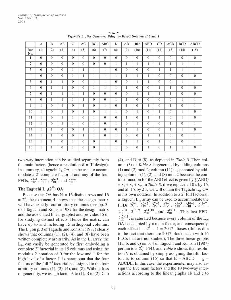
Journal of Manufacturing SystemsVol. 23/No. 22004
98
two-way interaction can be studied separately fromthe main factors (hence a resolution R = III design).In summary, a Taguchi L8 OA can be used to accom-modate a 23 complete factorial and any of the fourFFDs, 4 1
IV2 − , 5 2III2 − , 6 3
III2 − , and 7 4III2 − .
The Taguchi L16(215) OA
Because this OA has Nf = 16 distinct rows and 16= 24, the exponent 4 shows that the design matrixwill have exactly four arbitrary columns (see pp. 3-6 of Taguchi and Konishi 1987 for the design matrixand the associated linear graphs) and provides 15 dffor studying distinct effects. Hence the matrix canhave up to and including 15 orthogonal columns.The L16 on p. 3 of Taguchi and Konishi (1987) clearlyshows that columns (1), (2), (4), and (8) have beenwritten completely arbitrarily. As in the L8 array, theL16 can easily be generated by first embedding acomplete 24 factorial in its 15 columns and using themodulus 2 notation of 0 for the low and 1 for thehigh level of a factor. It is paramount that the fourfactors of the full 24 factorial be assigned to the fourarbitrary columns (1), (2), (4), and (8). Without lossof generality, we assign factor A to (1), B to (2), C to
(4), and D to (8), as depicted in Table 8. Then col-umn (3) of Table 8 is generated by adding columns(1) and (2) mod 2; column (11) is generated by add-ing columns (1), (2), and (8) mod 2 because the con-trast function for the ABD effect is given by �(ABD)= x1 + x2 + x4. In Table 8, if we replace all 0’s by 1’sand all 1’s by 2’s, we will obtain the Taguchi L16 OAin his own notation. In addition to a 24 full factorial,a Taguchi L16 array can be used to accommodate theFFDs 5 1
V2 − , 6 2IV2 − , 7 3
IV2 − , 8 4IV2 − , 9 5
III2 − , 10 6III2 − , 11 7
III2 − ,12 8III2 − , 13 9
III2 − , 14 10III2 − , and 15 11
III2 − . This last FFD,15 11III2 − , is saturated because every column of the L16
OA is occupied by a main factor, and consequently,each effect has 211 – 1 = 2047 aliases (this is dueto the fact that there are 2047 blocks each with 16FLCs that are not studied). The three linear graphs(1a, b, and c) on p. 4 of Taguchi and Konishi (1987)pertain to a 5 1
V2 − FFD, and Table 8 shows that resolu-tion V is obtained by simply assigning the fifth fac-tor, E, to column (15) so that E = ABCD Æ g =ABCDE. In this case, the experimenter may also as-sign the five main factors and the 10 two-way inter-actions according to the linear graphs 1b and c to
Table 8Taguchi’s L16 OA Generated Using the Base-2 Notation of 0 and 1
A B AB C AC BC ABC D AD BD ABD CD ACD BCD ABCD
Run No.
(1) (2) (3) (4) (5) (6) (7) (8) (9) (10) (11) (12) (13) (14) (15)
1 0 0 0 0 0 0 0 0 0 0 0 0 0 0 0
2 0 0 0 0 0 0 0 1 1 1 1 1 1 1 1
3 0 0 0 1 1 1 1 0 0 0 0 1 1 1 1
4 0 0 0 1 1 1 1 1 1 1 1 0 0 0 0
5 0 1 1 0 0 1 1 0 0 1 1 0 0 1 1
6 0 1 1 0 0 1 1 1 1 0 0 1 1 0 0
7 0 1 1 1 1 0 0 0 0 1 1 1 1 0 0
8 0 1 1 1 1 0 0 1 1 0 0 0 0 1 1
9 1 0 1 0 1 0 1 0 1 0 1 0 1 0 1
10 1 0 1 0 1 0 1 1 0 1 0 1 0 1 0
11 1 0 1 1 0 1 0 0 1 0 1 1 0 1 0
12 1 0 1 1 0 1 0 1 0 1 0 0 1 0 1
13 1 1 0 0 1 1 0 0 1 1 0 0 1 1 0
14 1 1 0 0 1 1 0 1 0 0 1 1 0 0 1
15 1 1 0 1 0 0 1 0 1 1 0 1 0 0 1
16 1 1 0 1 0 0 1 1 0 0 1 0 1 1 0
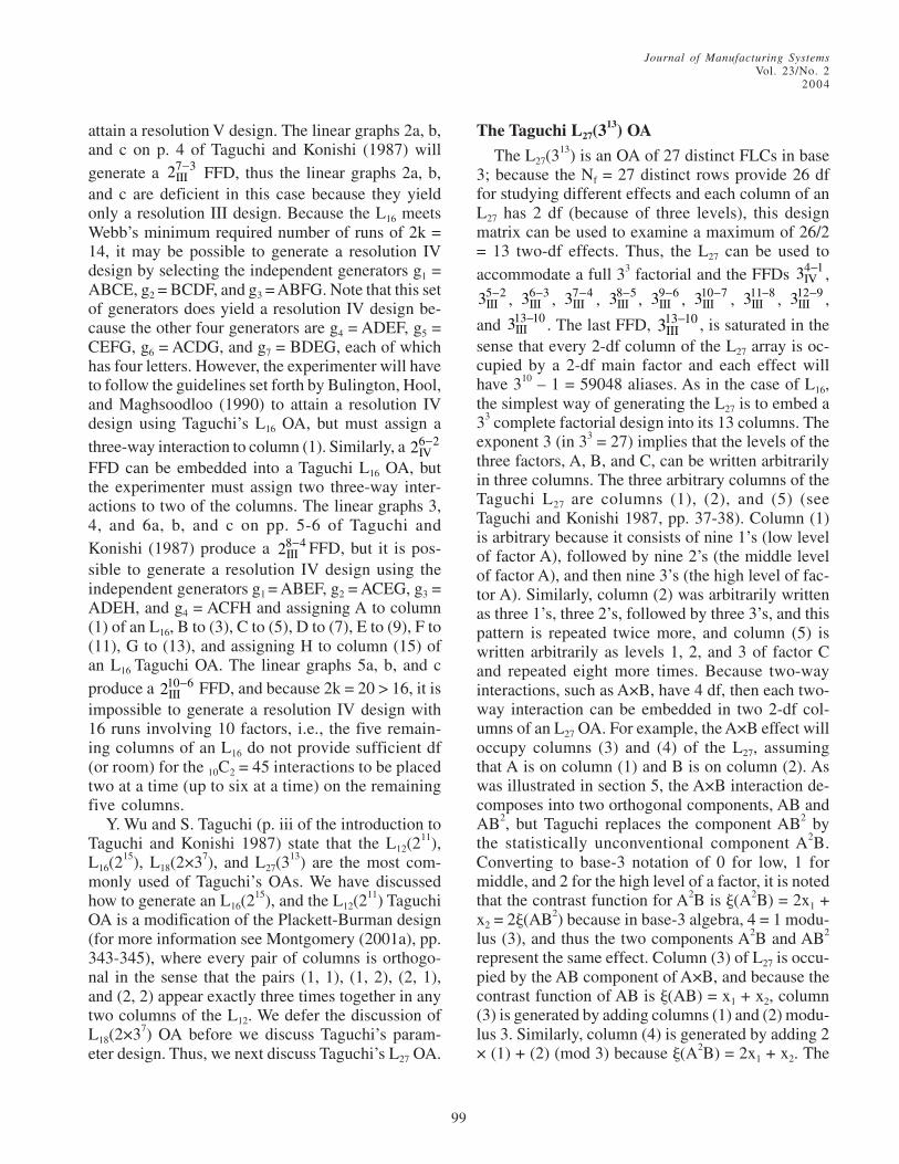
Journal of Manufacturing SystemsVol. 23/No. 2
2004
99
attain a resolution V design. The linear graphs 2a, b,and c on p. 4 of Taguchi and Konishi (1987) willgenerate a 7 3
III2 − FFD, thus the linear graphs 2a, b,and c are deficient in this case because they yieldonly a resolution III design. Because the L16 meetsWebb’s minimum required number of runs of 2k =14, it may be possible to generate a resolution IVdesign by selecting the independent generators g1 =ABCE, g2 = BCDF, and g3 = ABFG. Note that this setof generators does yield a resolution IV design be-cause the other four generators are g4 = ADEF, g5 =CEFG, g6 = ACDG, and g7 = BDEG, each of whichhas four letters. However, the experimenter will haveto follow the guidelines set forth by Bulington, Hool,and Maghsoodloo (1990) to attain a resolution IVdesign using Taguchi’s L16 OA, but must assign athree-way interaction to column (1). Similarly, a 6 2
IV2 −
FFD can be embedded into a Taguchi L16 OA, butthe experimenter must assign two three-way inter-actions to two of the columns. The linear graphs 3,4, and 6a, b, and c on pp. 5-6 of Taguchi andKonishi (1987) produce a 8 4
III2 − FFD, but it is pos-sible to generate a resolution IV design using theindependent generators g1 = ABEF, g2 = ACEG, g3 =ADEH, and g4 = ACFH and assigning A to column(1) of an L16, B to (3), C to (5), D to (7), E to (9), F to(11), G to (13), and assigning H to column (15) ofan L16 Taguchi OA. The linear graphs 5a, b, and cproduce a 10 6
III2 − FFD, and because 2k = 20 > 16, it isimpossible to generate a resolution IV design with16 runs involving 10 factors, i.e., the five remain-ing columns of an L16 do not provide sufficient df(or room) for the 10C2 = 45 interactions to be placedtwo at a time (up to six at a time) on the remainingfive columns.
Y. Wu and S. Taguchi (p. iii of the introduction toTaguchi and Konishi 1987) state that the L12(2
11),L16(2
15), L18(2×37), and L27(313) are the most com-
monly used of Taguchi’s OAs. We have discussedhow to generate an L16(2
15), and the L12(211) Taguchi
OA is a modification of the Plackett-Burman design(for more information see Montgomery (2001a), pp.343-345), where every pair of columns is orthogo-nal in the sense that the pairs (1, 1), (1, 2), (2, 1),and (2, 2) appear exactly three times together in anytwo columns of the L12. We defer the discussion ofL18(2×37) OA before we discuss Taguchi’s param-eter design. Thus, we next discuss Taguchi’s L27 OA.
The Taguchi L27(313) OA
The L27(313) is an OA of 27 distinct FLCs in base
3; because the Nf = 27 distinct rows provide 26 dffor studying different effects and each column of anL27 has 2 df (because of three levels), this designmatrix can be used to examine a maximum of 26/2= 13 two-df effects. Thus, the L27 can be used toaccommodate a full 33 factorial and the FFDs 4 1
IV3 − ,5 2III3 − , 6 3
III3 − , 7 4III3 − , 8 5
III3 − , 9 6III3 − , 10 7
III3 − , 11 8III3 − , 12 9
III3 − ,
and 13 10III3 − . The last FFD, 13 10
III3 − , is saturated in thesense that every 2-df column of the L27 array is oc-cupied by a 2-df main factor and each effect willhave 310 – 1 = 59048 aliases. As in the case of L16,the simplest way of generating the L27 is to embed a33 complete factorial design into its 13 columns. Theexponent 3 (in 33 = 27) implies that the levels of thethree factors, A, B, and C, can be written arbitrarilyin three columns. The three arbitrary columns of theTaguchi L27 are columns (1), (2), and (5) (seeTaguchi and Konishi 1987, pp. 37-38). Column (1)is arbitrary because it consists of nine 1’s (low levelof factor A), followed by nine 2’s (the middle levelof factor A), and then nine 3’s (the high level of fac-tor A). Similarly, column (2) was arbitrarily writtenas three 1’s, three 2’s, followed by three 3’s, and thispattern is repeated twice more, and column (5) iswritten arbitrarily as levels 1, 2, and 3 of factor Cand repeated eight more times. Because two-wayinteractions, such as A×B, have 4 df, then each two-way interaction can be embedded in two 2-df col-umns of an L27 OA. For example, the A×B effect willoccupy columns (3) and (4) of the L27, assumingthat A is on column (1) and B is on column (2). Aswas illustrated in section 5, the A×B interaction de-composes into two orthogonal components, AB andAB2, but Taguchi replaces the component AB2 bythe statistically unconventional component A2B.Converting to base-3 notation of 0 for low, 1 formiddle, and 2 for the high level of a factor, it is notedthat the contrast function for A2B is �(A2B) = 2x1 +x2 = 2�(AB2) because in base-3 algebra, 4 = 1 modu-lus (3), and thus the two components A2B and AB2
represent the same effect. Column (3) of L27 is occu-pied by the AB component of A×B, and because thecontrast function of AB is �(AB) = x1 + x2, column(3) is generated by adding columns (1) and (2) modu-lus 3. Similarly, column (4) is generated by adding 2× (1) + (2) (mod 3) because �(A2B) = 2x1 + x2. The

Journal of Manufacturing SystemsVol. 23/No. 22004
100
Microsoft Excel Mod function was used to gener-ate the entire L27 OA given in Table 9. If 0 is re-placed by 1, 1 by 2, and 2 by 3 in Table 9, Taguchi’sL27 OA in his own notation is obtained, as shownon p. 37 of Taguchi and Konishi (1987). The tableof interactions between two columns (TOIBTC) onp. 38 of Taguchi and Konishi (1987) assisted in
determining which second-order effect would oc-cupy which column of the L27 OA. The L27 OA canprovide a resolution IV design in only one instance,namely for the FFD 4 1
IV3 − , and to ensure that an R =IV is attained, all the experimenter has to do is as-sign the fourth factor D to one of the columns (9),(10), (12), or (13), while factors A, B, and C must
Table 9Generating Taguchi’s L27 Using Microsoft Excel Mod 3 Function
A B AB A2B C AC A2C BC ABC A2BC B2C AB2C A2B2C
Run No.
(1) (2) (3) (4) (5) (6) ('7) (8) (9) (10) (11) (12) (13)
1 0 0 0 0 0 0 0 0 0 0 0 0 0
2 0 0 0 0 1 1 1 1 1 1 1 1 1
3 0 0 0 0 2 2 2 2 2 2 2 2 2
4 0 1 1 1 0 0 0 1 1 1 2 2 2
5 0 1 1 1 1 1 1 2 2 2 0 0 0
6 0 1 1 1 2 2 2 0 0 0 1 1 1
7 0 2 2 2 0 0 0 2 2 2 1 1 1
8 0 2 2 2 1 1 1 0 0 0 2 2 2
9 0 2 2 2 2 2 2 1 1 1 0 0 0
10 1 0 1 2 0 1 2 0 1 2 0 1 2
11 1 0 1 2 1 2 0 1 2 0 1 2 0
12 1 0 1 2 2 0 1 2 0 1 2 0 1
13 1 1 2 0 0 1 2 1 2 0 2 0 1
14 1 1 2 0 1 2 0 2 0 1 0 1 2
15 1 1 2 0 2 0 1 0 1 2 1 2 0
16 1 2 0 1 0 1 2 2 0 1 1 2 0
17 1 2 0 1 1 2 0 0 1 2 2 0 1
18 1 2 0 1 2 0 1 1 2 0 0 1 2
19 2 0 2 1 0 2 1 0 2 1 0 2 1
20 2 0 2 1 1 0 2 1 0 2 1 0 2
21 2 0 2 1 2 1 0 2 1 0 2 1 0
22 2 1 0 2 0 2 1 1 0 2 2 1 0
23 2 1 0 2 1 0 2 2 1 0 0 2 1
24 2 1 0 2 2 1 0 0 2 1 1 0 2
25 2 2 1 0 0 2 1 2 1 0 1 0 2
26 2 2 1 0 1 0 2 0 2 1 2 1 0
27 2 2 1 0 2 1 0 1 0 2 0 2 1
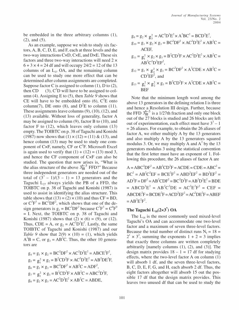
Journal of Manufacturing SystemsVol. 23/No. 2
2004
101
be embedded in the three arbitrary columns (1),(2), and (5).
As an example, suppose we wish to study six fac-tors, A, B, C, D, E, and F, each at three levels and thetwo-way interactions C×D, C×E, and D×E. These sixfactors and three two-way interactions will need 2 ×6 + 3 × 4 = 24 df and will occupy 24/2 = 12 of the 13columns of an L27 OA, and the remaining columncan be used to study one more effect that can bedetermined after column assignments are completed.Suppose factor C is assigned to column (1), D to (2),then CD Æ (3), C2D will have to be assigned to col-umn (4). Assigning E to (5), then Table 9 shows thatCE will have to be embedded onto (6), C2E ontocolumn(7), DE onto (8), and D2E to column (11).These assignments leave columns (9), (10), (12), and(13) available. Without loss of generality, factor Amay be assigned to column (9), factor B to (10), andfactor F to (12), which leaves only column (13)empty. The TOIBTC on p. 38 of Taguchi and Konishi(1987) now shows that (1) × (12) = (11) & (13), andhence column (13) may be used to study one com-ponent of C×F, namely, CF or C2F. Microsoft Excelis again used to verify that (1) + (12) = (13) mod 3,and hence the CF component of C×F can also bestudied. The question that now arises is, “What isthe alias structure of the above 6 3
III3 − FFD?” Becausethree independent generators are needed out of thetotal of (33 – 1)/(3 – 1) = 13 generators and theTaguchi L27 always yields the PB of a FFD, theTOIBTC on p. 38 of Taguchi and Konishi (1987) isused to assist in identifying the alias structure. Thistable shows that (13) = (2) × (10) and thus CF = BD,or C3F3 = BC2DF2, which shows that one of the de-sign generators is g1 = BC2DF2 because C3F3 = C0F0
= I. Next, the TOIBTC on p. 38 of Taguchi andKonishi (1987) shows that (2) × (6) = (9), or (12).Thus, CDE = A, or g2 = AC2D2E2. Lastly, the sameTOIBTC of Taguchi and Konishi (1987) and ourTable 9 show that 2(9) × (10) = (1), which yieldsA2B = C, or g3 = AB2C. Thus, the other 10 genera-tors are
g4 = g1 × g2 = BC2DF2 × AC2D2E2 = ABCE2F2,
g5 = 21g × g2 = B2CD2F × AC2D2E2 = AB2DE2F,
g6 = g1 × g3 = BC2DF2 × AB2C = ADF2,
g7 = 21g × g3 = B2CD2F × AB2C = ABC2D2F,
g8 = g2 × g3 = AC2D2E2 × AB2C = ABDE,
g9 = g2 × 23g = AC2D2E2 × A2BC2 = BCD2E2,
g10 = g1 × g2 × g3 = BC2DF2 × AC2D2E2 × AB2C =
ACEF,
g11 = 21g × g2 × g3 = B2CD2F × AC2D2E2 × AB2C =
AB2C2D2EF2,
g12 = g1 × 22g × g3 = BC2DF2 × A2CDE × AB2C =
CD2EF2, and
g13 = 21g ×
22g × g3 = B2CD2F × A2CDE × AB2C =
BEF
Note that the minimum length word among theabove 13 generators in the defining relation I is threeand hence a Resolution III design. Further, becausethe FFD 6 3
III3 − is a 1/27th fraction and only one blockout of the 27 blocks is studied and 26 blocks are leftout of experimentation, each effect must have 33 – 1= 26 aliases. For example, to obtain the 26 aliases offactor A, we either multiply A by the 13 generatorsand also multiply A by the 13 generators squaredmodulus 3. Or, we may multiply A and A2 by the 13generators modulus 3 using the statistical conventionthat the first letter must have an exponent of 1. Fol-lowing this procedure, the 26 aliases of factor A are
A = ABC2DF2 = AB2CD2F = ACDE = CDE = ABC2 =
BC2 = AB2C2EF = BCE2F2 = ABD2EF2 = BD2EF2 =
AD2F = DF2 = AB2CDF2 = BC2D2F = AB2D2E2 = BDE
= ABCD2E2 = AB2C2DE = AC2E2F2 = CEF =
ABCDE2F = BCDE2F = ACD2EF2 = AC2DE2F = ABEF
= AB2E2F2.
The Taguchi L18(2×37) OAThe L18 is the most commonly used mixed-level
Taguchi’s OA and can accommodate one two-levelfactor and a maximum of seven three-level factors.Because the total number of distinct runs Nf = 18 =21 × 32, summing the exponents 1 + 2 = 3 impliesthat exactly three columns are written completelyarbitrarily [namely columns (1), (2), and (3)]. Thedesign matrix provides 18 – 1 = 17 df for studyingeffects, where the two-level factor A on column (1)will absorb 1 df, and the seven three-level factors,B, C, D, E, F, G, and H, each absorb 2 df. Thus, theeight factors altogether will absorb 15 out the pos-sible 17 df that the design matrix provides. Thisleaves two unused df that can be used to study the

Journal of Manufacturing SystemsVol. 23/No. 22004
102
interaction only between columns (1) and (2). As-suming, without loss of generality, that A is the two-level factor, the experimenter must embed thethree-level factor whose interaction with factor A heor she would like to examine in column (2). Later itwill be shown in a parameter design example thatthe only possible interaction that can be studied is(1)×(2), but this interaction cannot be embedded intothe design matrix. The question that now arises ishow Dr. Taguchi developed the other five columns(4, 5, 6, 7, and 8) of the L18 so that the design matrixis orthogonal. As stated earlier, the first three col-umns are written completely arbitrarily. Then, weneed to address the construction of columns (4)through (8) of the L18. The reader must be informedthat we are not sure how G. Taguchi developed hisL18 OA, and what follows is our explanation. To thisend, let us define a group of three 3×1 vectors, G1 =
1
2
3
⎡ ⎤⎢ ⎥⎢ ⎥⎢ ⎥⎣ ⎦
= [ ]1 2 3 ′ , ′G2 = 2 3 1[ ], and ′G3 = 3 1 2[ ] ,
where prime is used to denote matrix transpose. Note
that column (3) of L18 is arbitrarily written as′ ′ ′ ′ ′ ′[ ]′G G G G G G1 1 1 1 1 1 . Next, the above three
vectors are translated by subtracting 2 from each el-ement so that G1 transforms to G4 = [ ]1 0 1 ′− , G2
transforms to G5 = [ ]0 1 1 ′− , and G3 translates to6G′ = 1 1 0−[ ] . (Note that G4 is the linear contrast
in base 3 for a quantitative factor.) It is well knownthat two vectors are orthogonal if and only if theirdot product is zero. Clearly, ′ ×G G4 5 = −[ ]1 0 1 ×0 1 1−[ ]′ = –1 = ′ ×G G64 = ′ ×G G5 6 , which implies
that the vectors G1 and G2 are not orthogonal, G1
and G3 are not orthogonal, and neither are G2 andG3. Further, ′ ×G Gi i = +2 for all i = 4, 5, and 6. Aclose examination of the fourth column of L18 on p.36 of Taguchi and Konishi (1987) reveals that col-umn (4) can be written as (4) =
′ ′ ′ ′ ′ ′[ ]′G G G G G G1 1 2 3 2 3 and column (5) of L18 issimply (5) = ′ ′ ′ ′ ′ ′[ ]′G G G G G G1 2 1 3 3 2 . If we nowtake the dot product of column (4) with (5) after thetranslation, we obtain ′ ′ ′ ′ ′ ′[ ]G G G G G G4 4 5 6 5 6 ×
G
G
G
G
G
G
4
5
4
6
6
5
⎡
⎣
⎢⎢⎢⎢⎢⎢⎢⎢
⎤
⎦
⎥⎥⎥⎥⎥⎥⎥⎥
= 2 – 1 – 1 + 2 – 1 – 1 = 0, which shows that
columns (4) and (5) of L18 are orthogonal. Anotherpattern that is obvious in the L18 is that columns (3)through (8) have their first three rows as the 3×1vector G1. To generate column (6), we have to findanother permutation of ′ ′ ′ ′ ′ ′[ ]′G G G G G G1 1 2 2 3 3 ,keeping G1 in the first position, which is orthogonalto both columns (4) and (5). One such permutationis ′ ′ ′ ′ ′ ′[ ]′G G G G G G1 2 3 2 1 3 , which comprises col-umn (6) of Taguchi’s L18. Similarly, two other per-mutations of ′ ′ ′ ′ ′ ′[ ]′G G G G G G1 1 2 2 3 3 that areorthogonal to columns (3), (4), (5), and (6) are col-umns (7) = ′ ′ ′ ′ ′ ′[ ]′G G G G G G1 3 2 2 3 1 and (8) =
′ ′ ′ ′ ′ ′[ ]′G G G G G G1 3 3 1 2 2 of Taguchi’s L18 OA. Thelast five columns of the L18 Taguchi OA in terms ofthe 3×1 vectors G1, G2, and G3 are given below anddenoted as the matrix G.
4 5 6 7 8
1 1 1 1 1
1 2 2 3 3
2 1 3 2 3
3 3 2 2 1
( ) ( ) ( ) ( ) ( )
=G
G G G G G
G G G G G
G G G G G
G G G G G
G22 3 1 3 2
3 2 3 1 2
G G G G
G G G G G
⎡
⎣
⎢⎢⎢⎢⎢⎢⎢⎢
⎤
⎦
⎥⎥⎥⎥⎥⎥⎥⎥
The above developments indicate that the L18 is notunique in the sense that there are other permutationsof the last five rows of the matrix G that yield an L18
orthogonal array. We have identified all other Gmatrices, of which there are 11, that are somewhatdistinct from the above Taguchi’s layout but willalso yield an L18 OA. The other 11 are listed atopthe next page. Note that the orthogonality of the 11alternatives to Taguchi’s L18 was verified by firstreplacing column (1) by nine –1’s followed by nine+1’s, then subtracting 2 from every element of theremaining seven columns so that all eight columnssummed to zero, and finally computing the result-ing X′×X matrix. In all the 11 alternative cases, theresulting 8×8 matrix X′×X was diagonal, andMinitab’s GLM also verified that all 11 design ma-trices were orthogonal.
7. Taguchi’s Parameter DesignA Taguchi parameter design experiment consists
of two orthogonal arrays. The inner array accom-

Journal of Manufacturing SystemsVol. 23/No. 2
2004
103
modates the controllable factors, while the noise (oruncontrollable) factors are embedded into the outerorthogonal array. The objectives of a PDE (parameterdesign experiment) for a nominal dimension is three-fold, the last two of which are optimization steps:
1. To classify the design factors into three catego-ries of Control, Signal, and Weak factors. A Con-
trol factor is one that impacts process variabil-ity and may or may not impact the process meanresponse. A Signal factor significantly impactsthe mean response but has no (or trivial) im-pact on the variability of the response. A Weakfactor has no impact on the mean or variabilityof the response.
( ) ( ) ( ) ( ) ( )1 1 1 1 1
2 2 1 3 3
2 3 3 2 1
3 1 2 2 3
1 3 2 3 2
3 2 3 1 2
4 5 6 7 8
G G G G G
G G G G G
G G G G G
G G G G G
G G G G G
G G G G G
⎡ ⎤⎢ ⎥⎢ ⎥⎢ ⎥⎢ ⎥⎢ ⎥⎢ ⎥⎢ ⎥⎢ ⎥⎣ ⎦
,
( ) ( ) ( ) ( ) ( )1 1 1 1 1
1 2 2 3 3
2 3 1 3 2
2 1 3 2 3
3 2 3 1 2
3 3 2 2 1
4 5 6 7 8
G G G G G
G G G G G
G G G G G
G G G G G
G G G G G
G G G G G
⎡ ⎤⎢ ⎥⎢ ⎥⎢ ⎥⎢ ⎥⎢ ⎥⎢ ⎥⎢ ⎥⎢ ⎥⎣ ⎦
,
( ) ( ) ( ) ( ) ( )1 1 1 1 1
1 2 2 3 3
3 3 2 2 1
3 2 3 1 2
2 1 3 2 3
2 3 1 3 2
4 5 6 7 8
G G G G G
G G G G G
G G G G G
G G G G G
G G G G G
G G G G G
⎡ ⎤⎢ ⎥⎢ ⎥⎢ ⎥⎢ ⎥⎢ ⎥⎢ ⎥⎢ ⎥⎢ ⎥⎣ ⎦
,
( ) ( ) ( ) ( ) ( )1 1 1 1 1
1 2 2 3 3
3 3 2 2 1
2 1 3 2 3
3 2 3 1 2
2 3 1 3 2
4 5 6 7 8
G G G G G
G G G G G
G G G G G
G G G G G
G G G G G
G G G G G
⎡ ⎤⎢ ⎥⎢ ⎥⎢ ⎥⎢ ⎥⎢ ⎥⎢ ⎥⎢ ⎥⎢ ⎥⎣ ⎦
,
( ) ( ) ( ) ( ) ( )1 1 1 1 1
2 1 3 2 3
1 2 2 3 3
2 3 1 3 2
3 3 2 2 1
3 2 3 1 2
4 5 6 7 8
G G G G G
G G G G G
G G G G G
G G G G G
G G G G G
G G G G G
⎡ ⎤⎢ ⎥⎢ ⎥⎢ ⎥⎢ ⎥⎢ ⎥⎢ ⎥⎢ ⎥⎢ ⎥⎣ ⎦
,
( ) ( ) ( ) ( ) ( )1 1 1 1 1
2 1 3 2 3
1 2 2 3 3
3 3 2 2 1
2 3 1 3 2
3 2 3 1 2
4 5 6 7 8
G G G G G
G G G G G
G G G G G
G G G G G
G G G G G
G G G G G
⎡ ⎤⎢ ⎥⎢ ⎥⎢ ⎥⎢ ⎥⎢ ⎥⎢ ⎥⎢ ⎥⎢ ⎥⎣ ⎦
,
( ) ( ) ( ) ( ) ( )1 1 1 1 1
2 2 3 3 1
2 3 2 1 3
1 3 3 2 2
3 1 2 3 2
3 2 1 2 3
4 5 6 7 8
G G G G G
G G G G G
G G G G G
G G G G G
G G G G G
G G G G G
⎡ ⎤⎢ ⎥⎢ ⎥⎢ ⎥⎢ ⎥⎢ ⎥⎢ ⎥⎢ ⎥⎢ ⎥⎣ ⎦
,
( ) ( ) ( ) ( ) ( )1 1 1 1 1
1 3 2 3 2
2 3 1 2 3
2 2 3 3 1
3 2 2 1 3
3 1 3 2 2
4 5 6 7 8
G G G G G
G G G G G
G G G G G
G G G G G
G G G G G
G G G G G
⎡ ⎤⎢ ⎥⎢ ⎥⎢ ⎥⎢ ⎥⎢ ⎥⎢ ⎥⎢ ⎥⎢ ⎥⎣ ⎦
,
( ) ( ) ( ) ( ) ( )1 1 1 1 1
1 3 2 2 3
3 1 2 3 2
3 2 3 2 1
2 2 1 3 3
2 3 3 1 2
4 5 6 7 8
G G G G G
G G G G G
G G G G G
G G G G G
G G G G G
G G G G G
⎡ ⎤⎢ ⎥⎢ ⎥⎢ ⎥⎢ ⎥⎢ ⎥⎢ ⎥⎢ ⎥⎢ ⎥⎣ ⎦
,
( ) ( ) ( ) ( ) ( )1 1 1 1 1
3 2 2 1 3
3 1 3 2 2
2 2 3 3 1
2 3 1 2 3
1 3 2 3 2
4 5 6 7 8
G G G G G
G G G G G
G G G G G
G G G G G
G G G G G
G G G G G
⎡ ⎤⎢ ⎥⎢ ⎥⎢ ⎥⎢ ⎥⎢ ⎥⎢ ⎥⎢ ⎥⎢ ⎥⎣ ⎦
,
( ) ( ) ( ) ( ) ( )1 1 1 1 1
2 2 3 1 3
3 2 1 3 2
3 1 2 2 3
2 3 2 3 1
1 3 3 2 2
4 5 6 7 8
G G G G G
G G G G G
G G G G G
G G G G G
G G G G G
G G G G G
⎡ ⎤⎢ ⎥⎢ ⎥⎢ ⎥⎢ ⎥⎢ ⎥⎢ ⎥⎢ ⎥⎢ ⎥⎣ ⎦

Journal of Manufacturing SystemsVol. 23/No. 22004
104
2. To use the levels of the Control factors to re-duce process variability.
3. To use the levels of Signal factors to move themean response toward the ideal target m.
When the response, y, is either STB or LTB, QI canbe accomplished in one step by increasing the sig-nal-to-noise ratio (which in turn lowers the signalfor an STB and heightens it for an LTB QCH), andas a result the experimenter can accomplish objec-tives (2) and (3) above in one step by setting theprocess conditions at those levels of influential fac-tors that maximize Taguchi’s S/N ratio, measured indecibels as defined below.
( )
( )
db 10
n2
10 ii 1
n2
10 ii 1
10 log MSD
10 log y n , if y is STB
110 log 1 y , if y LTB
n
=
=
η = − =
⎧ ⎛ ⎞− ∑⎜ ⎟⎪ ⎝ ⎠⎪⎨
⎡ ⎤⎪− ∑⎢ ⎥⎪ ⎣ ⎦⎩
It should be highlighted that classical design ofexperiments until the mid 1970s emphasized meth-ods that improve only the mean response, and henceone OA would generally be sufficient, and in somecases more efficient, to carry out QI only when theresponse y is STB or LTB. However, when the re-sponse is of nominal type, the variability of responseplays a very important role in QI, and hence an outerOA is needed to embed the noise factors that causeprocess variability. In a PDE, the experimenter in-tentionally induces noise into the response y throughthe use of an outer array and then takes advantageof the interactions between the noise factors in theouter array with the controllable factors in the innerarray to assess and then diminish the impact of noiseon the response y (using appropriate S/N ratios). Theimpact of noise factors is diminished by selectingthose levels of the controllable influential factors em-bedded in the inner OA that are less sensitive to noisefactors embedded in the outer array, thereby pro-ducing a more robust product.
To illustrate Taguchi’s PDE, we make use of aquality engineering experiment published by theAmerican Supplier Institute (ASI), Inc. (1984) fromits Seminar Series B. The nominal response variable,y, is the pull-force of ignition cables measured inpounds (lb). The specifications on y are 40 ± 15 lb,that is, the ideal target for pull-force is m = 40 lb and
the manufacturing (semi-) tolerance is � = 15 lb. Theexperimental layout and the resulting data are dis-played in Table 10. The controllable factors are A =extrusion tooling (two levels: type 1 and type 2), B= line speed (three levels: slow, medium, and fast),C = water through temperature (low, medium, high),D = insulation material (types 1, 2, and 3), E = CVstream pressure (low, medium, and high), F = CVspeed (slow, medium, fast), G = braid tension (low,medium, high), and H = release coating (types 1, 2,and 3). The noise factors are Sample (two cablesselected at random), P = position within each of thetwo sampled cables.
Note that we have borrowed, with permission, theexperimental layout and the data therein from theAmerican Supplier Institute, but all the analyses per-formed in Microsoft Excel, Matlab, and a Taguchisoftware belong to the authors. Table 10 shows thatrun number 1, where all factors were at their lowlevels, yielded much better results than run 2 be-cause all four measurements of pull-force in run 1were within the spec interval (LSL = 25, USL = 55lb). At run 2, where factors A and B were at lowwhile the other six factors were at their medium lev-els, the sample 1 at both positions gave two noncon-forming measurements (10 and 15 lb). Table 11 givesthe summary statistics for each run (i = 1, 2, …, 18),
where the grand total 18 4
.. iji=1 j 1
y y 3779=
= ∑∑ = . In Table 11,
the first-row statistics were computed as 1.y = (30 + 40
+ 38 + 49)/4 = 39.25, S1 = ( )4 2
1jj 1
1y 39.25
3 =∑ − =
7.80491, and �1 = 10×log10 21.21
y 1
S 4
⎛ ⎞−⎜ ⎟
⎝ ⎠ = 10×log10
(25.0397) = 13.9863, where the subscript i extendsover the FLCs 1 through 18 and j extends over thefour observations in the outer L4 OA. The last col-umn gives the natural logarithm of the i-th run stan-dard deviation.
We next use the summary statistics in Table 11 toobtain a response table (RT) for total S/N ratios thatwill help identify the factors that control processvariation. Microsoft Excel was used to obtain the RTfor S/N ratios, which is presented in Table 12a. Be-cause this is a mixed-level design, only MSs (meansquares) can be compared against each other to as-sess their relative influence on the S/N ratio of theresponse y. Table 12a clearly shows that factor Hhas the largest impact on the S/N ratio of the pull-
(4)

Journal of Manufacturing SystemsVol. 23/No. 2
2004
105
force and thus was assigned a rank of 1, and factorsA, C, and E have relatively trivial impact on the S/Nof the pull-force. The MSs in Table 12a indicate thatfactors H, B, D, and G are, in that order, relativelythe most influential from the standpoint of processvariation, and factor F moderately influences S/Nratio. Thus, the Control factors in the order of theirstrength are H, B, D, G, and F. Our experience indi-cates that most quantitative Control factors have aquadratic impact on the response and most Signalfactors have a linear impact on y (but not always).
Before deciding where to set the levels of thesefive Control factors, the reader should be remindedthat the L18 OA provides sufficient df to study onlythe interaction (1)×(2) = A×B. Factors A and B arecrossed to exhibit their interaction in Table 12b.From Table 12b, it is deduced that the effect of fac-
tor B on the S/N of y at A1 is positively quadratic(i.e., convex upward) given by Contrast(BA1) =48.15217 – 2(36.98029) + 54.34445 = 28.5360,and the quadratic effect of B at A2 is given byContrast(BA2) = 40.40491 – 2(31.19984) +55.08833 = 33.0936. Because these two quadraticcontrasts are quite similar, factors A and B do notmuch interact in impacting the S/N ratio of the re-sponse y. From Table 12b, the SS of A×B is givenby SS(A×B)� =
2 2 2 2 2 248.15217 36.98029 54.34445 40.40491 31.19984 55.08833
3
+ + + + + −
2266.1700
18 – SS(A�) – SS(B�) = 6.58524 Æ MS(A×B)�
= 3.292620, which again confirms that A and B donot materially interact in impacting the variability ofpull-force on a relative basis [see Table 12a thatshows MS(H�) = 81.7904].
Table 10PDE Layout from ASI, Inc. (reprinted with permission)
L18 Inner OA L4 Outer OA Taguchi’s
L18 OA A B C D E F G H Sample 1 Sample 2
Columns (1) (2) (3) (4) (5) (6) (7) (8) P1 P2 P1 P2
Run No.
1 1 1 1 1 1 1 1 1 30 lb 40 38 49
2 1 1 2 2 2 2 2 2 10 15 25 25
3 1 1 3 3 3 3 3 3 49 53 53 55
4 1 2 1 1 2 2 3 3 62 58 52 68
5 1 2 2 2 3 3 1 1 30 50 49 62
6 1 2 3 3 1 1 2 2 10 25 29 36
7 1 3 1 2 1 3 2 3 58 42 41 50
8 1 3 2 3 2 1 3 1 28 29 32 31
9 1 3 3 1 3 2 1 2 110 74 94 115
10 2 1 1 3 3 2 2 1 76 88 66 103
11 2 1 2 1 1 3 3 2 52 37 54 59
12 2 1 3 2 2 1 1 3 55 79 62 98
13 2 2 1 2 3 1 3 2 5 35 16 42
14 2 2 2 3 1 2 1 3 52 96 79 91
15 2 2 3 1 2 3 2 1 50 70 56 65
16 2 3 1 3 2 3 1 2 15 20 18 21
17 2 3 2 1 3 1 2 3 51 62 59 70
18 2 3 3 2 1 2 3 1 77 83 66 74
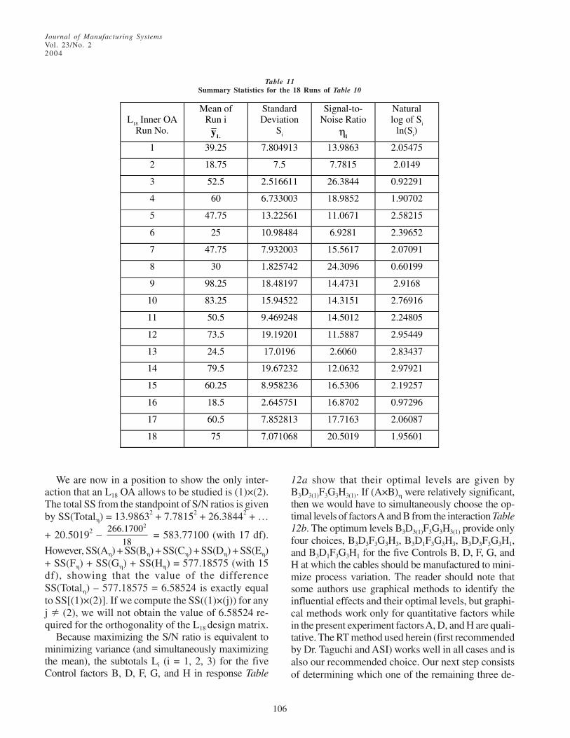
Journal of Manufacturing SystemsVol. 23/No. 22004
106
We are now in a position to show the only inter-action that an L18 OA allows to be studied is (1)×(2).The total SS from the standpoint of S/N ratios is givenby SS(Total�) = 13.98632 + 7.78152 + 26.38442 + …
+ 20.50192 – 2266.1700
18 = 583.77100 (with 17 df).
However, SS(A�) + SS(B�) + SS(C�) + SS(D�) + SS(E�)+ SS(F�) + SS(G�) + SS(H�) = 577.18575 (with 15df), showing that the value of the differenceSS(Total�) – 577.18575 = 6.58524 is exactly equalto SS[(1)×(2)]. If we compute the SS((1)×(j)) for anyj � (2), we will not obtain the value of 6.58524 re-quired for the orthogonality of the L18 design matrix.
Because maximizing the S/N ratio is equivalent tominimizing variance (and simultaneously maximizingthe mean), the subtotals Li (i = 1, 2, 3) for the fiveControl factors B, D, F, G, and H in response Table
12a show that their optimal levels are given byB3D3(1)F3G3H3(1). If (A×B)� were relatively significant,then we would have to simultaneously choose the op-timal levels of factors A and B from the interaction Table12b. The optimum levels B3D3(1)F3G3H3(1) provide onlyfour choices, B3D3F3G3H3, B3D1F3G3H3, B3D3F3G3H1,and B3D1F3G3H1 for the five Controls B, D, F, G, andH at which the cables should be manufactured to mini-mize process variation. The reader should note thatsome authors use graphical methods to identify theinfluential effects and their optimal levels, but graphi-cal methods work only for quantitative factors whilein the present experiment factors A, D, and H are quali-tative. The RT method used herein (first recommendedby Dr. Taguchi and ASI) works well in all cases and isalso our recommended choice. Our next step consistsof determining which one of the remaining three de-
Table 11Summary Statistics for the 18 Runs of Table 10
L18 Inner OA
Run No.
Mean of Run i
i .y
Standard Deviation
Si
Signal-to- Noise Ratio
iη
Natural log of Si
ln(Si)
1 39.25 7.804913 13.9863 2.05475
2 18.75 7.5 7.7815 2.0149
3 52.5 2.516611 26.3844 0.92291
4 60 6.733003 18.9852 1.90702
5 47.75 13.22561 11.0671 2.58215
6 25 10.98484 6.9281 2.39652
7 47.75 7.932003 15.5617 2.07091
8 30 1.825742 24.3096 0.60199
9 98.25 18.48197 14.4731 2.9168
10 83.25 15.94522 14.3151 2.76916
11 50.5 9.469248 14.5012 2.24805
12 73.5 19.19201 11.5887 2.95449
13 24.5 17.0196 2.6060 2.83437
14 79.5 19.67232 12.0632 2.97921
15 60.25 8.958236 16.5306 2.19257
16 18.5 2.645751 16.8702 0.97296
17 60.5 7.852813 17.7163 2.06087
18 75 7.071068 20.5019 1.95601

Journal of Manufacturing SystemsVol. 23/No. 2
2004
107
sign factors, A, C, and E, have large impacts on themean of y and using their levels to adjust the meantoward the ideal target of m = 40 lb.
To ascertain which design factors have nontrivialimpact on the mean, we have made a RT for themean of pull-force, which is provided in Table 13a.In Table 13a, rank 5 is missing because the ANOVAtable from Minitab, given below, shows that A×B isthe fifth most statistically significant effect that af-fects the mean response, as illustrated in Table 13b.Table 13b clearly shows that the impact of factor Bon the mean response is positively linear at the lowlevel of A, but its impact has a negative slope at A2,and hence factors A and B interact in impacting themean response.
General Linear Model: y vs. A, B, A*B, C, D, E,F, G, H, Sample, Position, Sample*PositionFactor Type Levels ValuesA fixed 2 1, 2,B fixed 3 1, 2, 3C fixed 3 1, 2, 3D fixed 3 1, 2, 3E fixed 3 1, 2, 3F fixed 3 1, 2, 3G fixed 3 1, 2, 3H fixed 3 1, 2, 3Sample random 2 1, 2Position random 2 1, 2
Analysis of Variance for y, using Adjusted SS for Tests
Source DF Seq SS Adj SS Adj MS F PA 1 2508.7 2508.7 2508.7 26.97 0.000B 2 371.0 371.0 185.5 1.99 0.147A*B 2 4715.9 4715.9 2357.9 25.35 0.000C 2 4904.9 4904.9 2452.4 26.36 0.000D 2 2898.8 2898.8 1449.4 15.58 0.000E 2 3732.0 3732.0 1866.0 20.06 0.000F 2 10166.8 10166.8 5083.4 54.64 0.000G 2 1753.0 1753.0 876.5 9.42 0.000H 2 6794.7 6794.7 3397.3 36.52 0.000Sample 1 715.7 715.7 715.7 6.51 0.238Position 1 1810.0 1810.0 1810.0 16.45 0.154Sample* 1 110.0 110.0 110.0 1.18 0.282 PositionError 51 4744.5 4744.5 93.0Total 71 45226.0
S = 9.64522 R-Sq = 89.51% R-Sq(adj) = 85.40%
The above ANOVA table from Minitab verifies thatthe impact of factor B on the mean response is notsignificant, but factors A, C, and E do significantlyimpact (all three P-values < 0.0001) the mean pull-force. Therefore, A, C, and E qualify as Signal (oradjustment) factors, and their levels can be used toadjust the mean response toward the ideal target of40 lb. Note that even if the impact of factors D, F, G,and H on the mean response are highly statisticallysignificant, their levels cannot be adjusted becausethese four factors are Controls and their levels mustbe set according to maximizing the S/N ratio of theprocess to reduce variance.
Further, the above Minitab output can be used toverify the fact that the only interaction that can bestudied with an L18 OA is (1)×(2). In fact, we ranMinitab’s GLM and requested the Model terms A, B,C, A×C, D, E, F, G, H, Sample, Position, andSample×Position, but Minitab would not even pro-vide a meaningful ANOVA table due to the loss oforthogonality. The corresponding Minitab output isprovided below.
Effects A B C D E F G H
L1 139.4769 88.5571 82.3244 96.1926 83.5424 77.1349 80.0485 100.7105
L2 126.6931 68.1801 87.4389 69.1068 96.0658 88.1199 78.8333 63.16
L3 N/A 109.4328 96.4067 100.8706 86.5618 100.9152 107.2882 102.2994
SS 9.0792 141.822 16.9383 98.0253 14.2376 47.216 86.2863 163.5809
MS 9.0792 70.911 8.4692 49.0127 7.1188 23.608 43.1431 81.7904
Ranks 6 2 7 3 8 5 4 1
B1 B2 B3
A1 48.15217 36.98029 54.34445
A2 40.40491 31.19984 55.08833
Table 12aResponse Table for S/N Ratio in dB
Table 12bA×B Interaction for �dB

Journal of Manufacturing SystemsVol. 23/No. 22004
108
General Linear Model: y vs. A, B, C, A×C, D, E,F, G, H, Sample, Position
Factor Type Levels ValuesA fixed 2 1, 2,B fixed 3 1, 2, 3C fixed 3 1, 2, 3D fixed 3 1, 2, 3E fixed 3 1, 2, 3F fixed 3 1, 2, 3G fixed 3 1, 2, 3H fixed 3 1, 2, 3Sample random 2 1, 2Position random 2 1, 2
Analysis of Variance for y, using Adjusted SSfor Tests
Source Model DF Reduced DF Seq SSA 1 1 2508.7B 2 2 371.0A*C 2 2 4395.0C 2 2 4904.9D 2 2 364.7E 2 2 8665.8F 2 2 10166.8G 2 2 1753.0H 2 0+ 0.0Sample 1 1 715.7Position 1 1 1810.0Sample*Position 1 1 110.0Error 51 53 9460.4Total 71 71 45226.0
+ Rank deficiency due to empty cells, unbal-anced nesting, collinearity, or an undeclaredcovariate. No storage of results or furtheranalysis will be done.
S = 13.3603 R-Sq = 79.08% R-Sq(adj) = 71.98%
The above Minitab output clearly indicates that A×B= (1)×(2) is the only interaction that can be studied
with a Taguchi L18 OA and that the request for anyother interaction will lead to a non-orthogonal (ornon-additive) SS, most of which will be erroneous.
Before searching for the optimum, it must be men-tioned that G. Taguchi defines a measure called Sen-sitivity for a nominal dimension as SmdB =
10×log10(CF) = 10×log10 ( )2n y⎡ ⎤⎣ ⎦
= 20×log10 ( )y n
= 10×log10
2n
jj 1
y n=
⎡ ⎤⎛ ⎞∑⎢ ⎥⎜ ⎟⎝ ⎠⎢ ⎥⎣ ⎦
, which is clearly a logarithmic
transformation of the sample mean. The main utilityof Sensitivity is to use its ANOVA table to identifythe Signal factors. We would recommend against theuse of Taguchi’s SmdB because the RT for the meanand the corresponding ANOVA (see below Table12b) not only identify Signal factors but the RT forthe mean has the added utility of aiding the experi-menter in adjusting the mean toward the ideal targetm. The variance-reduction logarithmic transforma-
tion, SmdB = 10×log10 ( )2n y⎡ ⎤⎣ ⎦ , recommended by
Taguchi is sometimes needed when data are not nor-mally distributed, but the F tests in ANOVA are fairlyrobust and can withstand moderate departures of datafrom normality.
8. Identifying the Optimal Condition XO
We have partially identified the optimal levels ofsome of the process parameters such as Line Speedat its third level, Insulation Material either type 1 or3, CV Speed at the level Fast, Braid Tension at High,and Release Coating that must be set at either Low(type 1) or High (type 3). To identify the optimallevels of the Signal factors A, C, and E, we have atwo-fold problem:
1. At what FLC was the process being run be-fore PDE and thus what is the mean of theexisting process condition and the resultingsocietal QLs?
Effects A B C D E F G H
L1 46.58333 52.95833 45.54167 61.45833 52.83333 42.125 59.45833 55.91667
L2 58.38889 49.5 47.83333 47.875 43.5 69.125 49.25 39.25
L3 N/A 55 64.08333 48.125 61.125 46.20833 48.75 62.29167
Ranks 3 9 4 7 6 1 8 2
Table 13aResponse Table for the Mean in Pounds
Table 13bA×B Interaction Table Based on Means
B1 B2 B3
A1 36.83333 44.25000 58.66667
A2 69.08333 54.75000 51.33333
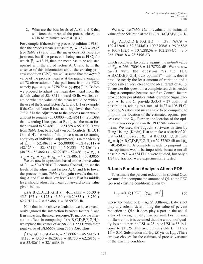
Journal of Manufacturing SystemsVol. 23/No. 2
2004
109
2. What are the best levels of A, C, and E thatwill force the mean of the process closest to40 lb to minimize societal QLs?
For example, if the existing process condition is FLC1,then the process mean is close to 1.y = 157/4 = 39.25(see Table 11) and thus the mean does not need ad-justment, but if the process is being run at FLC2 forwhich 2.y = 18.75, then the mean has to be adjustedupward with the aid of factors A, C, and E. In theabsence of this information about the existing pro-cess condition (EPC), we will assume that the defaultvalue of the process mean is at the grand average ofall 72 observations of the pull-force from the PDE,namely µEPC � y = 3779/72 = 52.48611 lb. Beforewe proceed to adjust the mean downward from thedefault value of 52.48611 toward 40 lb, we first ex-amine what the value of the mean would be withoutthe use of the Signal factors A, C, and E. For example,if the Control factor B is set at its high level, then fromTable 13a the adjustment to the process mean wouldamount to roughly (55.00000 – 52.48611) = 2.51389,that is, setting Line speed at B3 adjusts the mean fur-ther upward to 52.48611 + 2.51389 = 55.0000. Thus,from Table 13a, based only on our Controls (B, D, F,G, and H), the value of the process mean (assumingadditivity of individual adjustments) is in the vicinityof CTµ = 52.48611 + (55.00000 – 52.48611) +(48.12500 – 52.48611) + (46.20833 – 52.48611) +(48.75 – 52.48611) + 62.29167 – 52.48611) = B3y +
D3y + F3y + G3y + H3y – 4 × 52.48611 = 50.43056.We are now in a position, based on the above value
of µCT = 50.43056 (CT denotes Control), to set thelevels of the adjustment factors A, C, and E to lowerthe process mean. Table 13a again reveals that set-ting A and C at their low levels and E at its middlelevel should adjust the mean downward to the valuegiven below.
µ (A1B3C1D3E2F3G3H3) = 46.58333 + 55.00 +45.54167 + 48.125 + 43.50 + 46.20833 + 48.750 +62.29167 – 7 × 52.48611 = 28.59723 lb
Note that in the above calculation we have errone-ously ignored the interaction between factors A andB in impacting the mean response. To include the inter-action effect in computing µ (A1B3C1D3E2F3G3H3),we replace the values of 46.58333 + 55.00 with theirjoint value of 58.66667 from Table 13b. Thus,
µ (A1B3C1D3E2F3G3H3) = 58.66667 + 45.54167 +48.125 + 43.50 + 46.20833 + 48.750 + 62.29167 –6 × 52.48611 = 38.16668 lb
We now use Table 12a to evaluate the estimatedvalue of the S/N ratio at the FLC A1B3C1D3E2F3G3H3.
ηdB (A1B3C1D3E2F3G3H3) = 139.4769/9 +109.4328/6 + 82.3244/6 + 100.8706/6 + 96.0658/6+ 100.9152/6 + 107.2882/6 + 102.2994/6 – 7 ×266.1700/18 = 28.5196 dB
which compares favorably against the default valueof ηdB = 266.1700/18 = 14.78722 dB. We are nowfaced with the question “is the FLCA1B3C1D3E2F3G3H3 truly optimal?”—that is, does itproduce nearly the least amount of variation and aprocess mean very close to the ideal target of 40 lb.To answer this question, a complete search is neededusing a computer because our five Control factorsprovide four possibilities, while our three Signal fac-tors, A, E, and C, provide 3×3×3 = 27 additionalpossibilities, adding to a total of 4×27 = 108 FLCswhose S/N ratios and means have to be computed topinpoint the location of the estimated optimal pro-cess condition XO. Further, the location of the opti-mum always depends on the PEC S/N ratio and themean. We used the Taguchi software written byHung-Hsiang (Kevin) Hsu to make a search of XO
that yielded the result XO = A1B3C2D3E2F3G3H3 withηO = η(A1B3C2D3E2F3G3H3) = 29.37202 dB and µO
= 40.45834 lb. A complete search to pinpoint thetrue optimum would be impossible because not allpossible 2×37 = 4374 FLCs were studied, but only a1/243rd fraction were experimentally tested.
9. Loss Function Analysis After a PDETo estimate the percent reduction in societal QLs,
we must first compute the amount of QL at the PEC(present existing condition) given by
( ) ( )22PEC n PECL k S PEC y m⎡ ⎤= + −⎣ ⎦ (5)
where the value of k = Ac/�2. Although k does not
play any role in determining the value of percentreduction in QLs, it does play a part in the actualvalue of average quality loss per unit. For the sakeof illustration, it is assumed that the amount of qual-ity loss at either the LSL = 25 lb or USL = 55 lb isequal to $11.25. This assumption yields k = 11.25/152 = 0.05. Substitution into Eq. (5) yields LPEC . Thereare two choices for the estimate of process varianceof the existing condition:
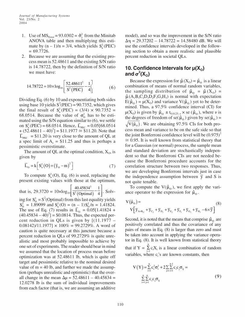
Journal of Manufacturing SystemsVol. 23/No. 22004
110
1. Use of MSError = 93.0302 = σy2 from the Minitab
ANOVA table and then multiplying this esti-mate by (n – 1)/n = 3/4, which yields Sn
2 (PEC)= 69.7726.
2. Because we are assuming that the existing pro-cess mean is 52.48611 and the existing S/N ratiois 14.78722, then by the definition of S/N ratiowe must have:
( )2
10 2
52.48611 114.78722 10 log
S PEC 4
⎡ ⎤= × −⎢ ⎥
⎢ ⎥⎣ ⎦ (6)
Dividing Eq. (6) by 10 and exponentiating both sidesusing base 10 yields S2(PEC) = 90.7352, which givesthe final result of Sn
2 (PEC) = (3/4) × 90.7352 =68.0514. Because the value of σO
2 has to be esti-mated using the S/N equation similar to (6), we settleon Sn
2 (PEC) = 68.0514. Hence, LPEC = 0.05[68.0514+ (52.48611 – 40)2] = $11.1977 � $11.20. Note thatLPEC = $11.20 is very close to the amount of QL ata spec limit of Ac = $11.25 and thus is perhaps apessimistic overestimate.
The amount of QL at the optimal condition, XO, isgiven by
( ) ( )22O n OL k S O y m⎡ ⎤= + −⎣ ⎦ (7)
To compute Sn2 (O), Eq. (6) is used, replacing the
present existing values with those at the optimum,
that is, 29.3720 = 10×log10
40 45834 1
4
2.
S Optimal2 ( ) −⎡
⎣⎢⎢
⎤
⎦⎥⎥
. Solv-
ing for SO2 = S2(Optimal) from this last equality yields
SO2 = 1.89099 and Sn
2 (O) = (n – 1)SO2 /n = 1.41824.
The use of Eq. (7) results in LO = 0.05[1.41824 +(40.45834 – 40)2] = $0.0814. Thus, the expected per-cent reduction in QLs is given by [(11.1977 –0.08142)/11.1977] × 100% = 99.2729%. A word ofcaution is quite necessary at this juncture because apercent reduction in QLs of 99.2729% is quite unre-alistic and most probably impossible to achieve byone set of experiments. The reader should bear in mindwe assumed that the location of process mean beforeoptimization was at 52.48611 lb, which is quite offtarget and pessimistic relative to the nominal desiredvalue of m = 40 lb, and further we made the assump-tion (perhaps unrealistic and optimistic) that the over-all change in the mean �µ = 52.48611 – 40.45834 =12.0278 lb is the sum of individual improvementsfrom each factor (that is, we are assuming an additive
model), and so was the improvement in the S/N ratio�� = 29.37202 – 14.78722 = 14.58480 dB. We willuse the confidence intervals developed in the follow-ing section to obtain a more realistic and plausiblepercent reduction in societal QLs.
10. Confidence Intervals for µ(XO)and �����2(XO)
Because the expression for µ (XO) = µO is a linearcombination of means of normal random variables,the sampling distribution of µO = µ (XO) =µ (A1B3C2D3D2F3G3H3) is normal with expectationE( µO ) = µ(XO) and variance V( µO ) yet to be deter-mined. Thus, a 97.5% confidence interval (CI) forµ(XO) is given by µO ± t0.0125; � × se ( µO ), where � isthe degrees of freedom of se( µO ) given by se( µO ) =
V Oµ( ) . We are obtaining 97.5% CIs for both pro-cess mean and variance to be on the safe side so thatthe joint Bonferroni confidence level will be (0.975)2
� 0.95. It is well known from statistical theory thatfor a Gaussian (or normal) process, the sample meanand standard deviation are stochastically indepen-dent so that the Bonferroni CIs are not needed be-cause the Bonferroni procedure accounts for thecorrelation structure between two responses. Thus,we are developing Bonferroni intervals just in casethe independence assumption between y and S isnot quite tenable.
To compute the V( µO ), we first apply the vari-ance operator to the expression for µO .
V
V y y y y y y y y
O
A B C D E F G H13 2 3 2 3 3 3
µ( ) =
+ + + + + + − ×⎡⎣ ⎤⎦× 6 (8)
Second, it is noted that the means that comprise µO arepositively correlated and thus the covariance of anypairs of means in Eq. (8) is larger than zero and mustbe taken into account in applying the variance opera-tor in Eq. (8). It is well known from statistical theory
that if Y = ∑=i
n
1ciXi is a linear combination of random
variables, where ci’s are known constants, then
( )n n-1
2 2i i i j ij
i 1 j>i i 1
n n
i j iji 1 j 1
V Y c 2 c c
c c
= =
= =
= ∑ σ + ∑∑ σ =
∑∑ σ (9)

Journal of Manufacturing SystemsVol. 23/No. 2
2004
111
where �ij = the covariance between Xi and Xj =E[(Xi – µi) × (Xj – µj)], i � j, �ii = σi
2 = V(Xi), and µi
= E(Xi). Further, if Xi’s that comprise the sum Y areall normally distributed, then the sampling distribu-tion of Y itself is Gaussian regardless of the correla-tion structure among all distinct pairs of Xi’s. For aproof of Eq. (9), the interested reader is referred towww.eng.auburn.edu/~maghsood/homepage.html,STAT 3600, Chapter 5, pp. 88-89.
Comparing Eq. (8) with (9), it is noted that c1 = c2 =c3 = c4 = c5 = c6 = c7 = 1 and c8 = –6. We now computethe variances and covariances of the eight means inEq. (8) term by term.
V y V y12
V y V1
24y
A Bj
12
A B jy2
Cj
13 1 3
2
×=
=
( ) = ∑⎛⎝⎜
⎞⎠⎟
=
( ) = ∑
1
1
24
1
12 , ;σ
CC jy2
2, 24⎛⎝⎜
⎞⎠⎟
=σ
;
similarly, V ( )3Dy = V ( )
2Ey = V ( )3Fy = V ( )
3Gy =
V( )3Hy =
2y
24
σ, and V(–6× y ) = 36
2y
72
⎛ ⎞σ⎜ ⎟⎜ ⎟⎝ ⎠
. The covariance
between 13A By × and
2Cy is Cov ( )13 2A B Cy , y× =
Cov 1 3 2
12 24
A B ,j C ,jj 1 j 1
1 1y , y
12 24= =
⎛ ⎞∑ ∑⎜ ⎟⎝ ⎠
. To carry out this last covari-
ance operation, it is noted that out of the 12 yij’s thatcomprise
13A By × exactly four of them are the same ob-servations as the 24 observations that comprise
2Cy ,and thus Cov ( )
13 2A B Cy ,y× = (1/12) × (1/24) × 4 2yσ =
2y
72
σ; similarly, the covariance of
13A By × with 3Dy ,
2Ey , 3Fy ,
3Gy , and 3Hy is also equal to
2y
72
σ.
The covariance between 13A By × and –6× y is given
by Cov ( )13A By , 6 y× − × = Cov 1 3
12 18 4
A B ,j ijj 1 i 1 j 1
1 6y , y
12 72= = =
−⎛ ⎞∑ ∑∑⎜ ⎟⎝ ⎠
=
(1/12)(–6/72)(12) 2yσ = (–6/72) 2
yσ . Similarly,
Cov ( )2Cy , 6 y− × =
2y6
72
− σ. Combining Eqs. (8) and (9),
we obtain the result V ( )Oµ = 2y
12
σ + 6 ×
2y
24
σ + 36 ×
2y
72
σ + 2
2 2y y
7 2
6C 7
72 72
⎡ ⎤σ − σ× + ×⎢ ⎥
⎢ ⎥⎣ ⎦ =
2y10
12
σ +
22 2y y67 6
72 72 72
⎡ ⎤σ − σ× × + ×⎢ ⎥⎢ ⎥⎣ ⎦
= 2y10
12
σ + 2
2y21
72
⎛ ⎞− σ⎜ ⎟⎜ ⎟⎝ ⎠
= 2y
4
σ.
This last result is intuitively appealing because X0
is an FLC and there were n = 4 observations at each
FLC, and it is well known that V ( )y = ( )V y
n =
2y
4
σ.
Because 2yσ is unknown, it must be estimated from
the gathered data. We have two choices, namely theMSError = 93.0302 from the Minitab ANOVA tablewith 51 df, or the estimate of the optimal varianceSO
2 = 1.89099 with 3 df. Because Oµ is the estimatedmean at the optimum, the estimated variance at theoptimum is the more logical choice, that is, σy
2 =SO
2 = 1.89099. Therefore, the standard error is given
by se µO( ) = σy
2
4 �
1
22SO =
1 89099
2
. = 0.6876,
and the 97.5% confidence interval for µO is givenby 40.45834 ± 4.1765 × 0.6876 = (37.5867,43.3300), where 4.1765 = t0.0125; 3 = the inverse ofW.S. Gosset’s t-distribution with 3 df at a cumula-tive of 0.9875.
Dr. Taguchi highly recommends that once the opti-mal condition XO is identified, the experimenter shouldconduct several confirmation runs at the optimal FLCbecause of the fact that only 18 out of the possible4374 FLCs were experimentally tested. Before con-ducting confirming experiments, one should note if theoptimal condition XO = A1B3C2D3E2F3G3H3 is one ofthe FLCs that was studied using the L18 OA. A com-parison of XO with the 18 FLCs of the L18 design ma-trix reveals that A1B3C2D3E2F3G3H3 is not one of theFLCs that was included in the L18. Note that the 18runs that were studied are just a 1/243rd fraction of all2×37 = 4374 possible distinct FLCs. Thus, in this case,Dr. Taguchi recommends that we set the process at XO
= A1B3C2D3E2F3G3H3 and make (at least) two cables,measure the pull-force at two positions, and computethe mean of the four measurements denoted by yCN ,where CN represents confirmation. We may use eitherthe inexact decision rule that if yCN falls inside the 97.5%CI (37.5867, 43.3300), then there should be no con-cern about XO from the standpoint of the mean; or wemay compare yCN against the decision interval40.45834 ± t0.025; � × se( yCN ). The experimenter shouldalso be cognizant of the fact that the confidence bandagainst which the future confirmation mean is to becompared should actually be wider than (37.5867,43.3300) because the confirmation runs will also haveexperimental error that is not included in the computa-tion of the CI (37.5867, 43.3300), which includes onlythe model error.

Journal of Manufacturing SystemsVol. 23/No. 22004
112
To arrive at an upper 97.5% CI for �2(XO) = σO2 ,
we make use of the fact that the sampling distribu-tion of (n – 1)SO
2 /σO2 is chi-squared with 3 df, as-
suming that n = 4. Thus, the upper 97.5% confidence
limit for σO2 is given by σO
2 (U) = n SO−( )1 2
0 975 32χ . ;
=
3 1 89099
0 2158
× .
. = 26.2887, that is, 0 < σO
2 � 26.2887 at
the 97.5% confidence level. Again, if the variance
found through confirmation experiments lies withinthe CI, 0 < σO
2 � 26.2887, then the optimal condi-tion is practically (not exactly from a statistical view-point) confirmed from the standpoint of variabilitybecause this CI includes only the model error.
11. Further Loss Function AnalysisIn section 9, we computed an unrealistic percent
reduction in QLs as 99.2729% that was, to say theleast, very optimistic. We now use the results of theCIs from section 10 to obtain a more realistic valuefor the percent reduction in QLs. To accomplish thisobjective, we use the worst-case scenarios for themean within the CI (37.5867, 43.3300), namely µO
= 43.3300, and also for the variance we will use theworst-case σO
2 = 26.2887. These yield an expectedQL at the optimal condition as LO(U) = 0.05 [26.2887+ (43.3300 – 40)2] = $1.8689. This leads to a per-cent reduction of [(11.1977 – 1.8689)/11.1977] ×100% = 83.31%. Because the two confidence bandseach were at the 97.5% level, we would have aBonferroni confidence level of (0.975)2 � 95% inthe percent QL reduction interval (83.31, 99.273%).Again, even the expected 83.31% reduction in QLsis overly optimistic and is due to the fact that we areusing the default value of y = 52.48611 lb for theexisting mean and the default value of S PECn
2 ( ) =68.0514. This brings us to the point that is impor-tant experimentally, and that is, if at all possible,one of the experimental runs should generally bethe FLC at which the process is presently being runso that the experimenter would have a good ideaabout the mean and S/N ratio of the existing pro-cess before optimization. Most design matrices af-ford sufficient flexibility to embed the existingcondition in the design matrix, but this is some-times impossible. Our 11 alternatives to Taguchi’sL18 in section 6 should help in this regard. For ex-ample, if run number 7 (see Table 11) in the L18 OAis the PEC of the process, then from Table 11 we
obtain LPEC = 0.05 [62.9167 + (47.75 – 40)2] =$6.1490, which leads to a more realistic percent re-duction in QLs of 69.61%. From the above discus-sions, if the optimal condition XO is verified throughconfirmation experiments for the design matrix ofTable 10, then we should expect more than a 50%reduction in QLs from the above optimization pro-cedure and no further analysis is needed. Otherwise,we will also need to reexamine our analyses accord-ing to the following section, and we should ponderthe possibility that there may be active interactionsin the process that were left out in the design phaseof the experiment.
12. Further Analysis of Data from a PDEOne warranted criticism of Taguchi methods by
most Western statisticians is the use of the S/N ratiofor analyzing data from a DOE. Because the samplemean and variance, when sampling a normal pro-cess, are stochastically independent, the recommen-dation from the statistical community is to analyzethe mean and variance separately. This is the reasonthat in Table 11 we provided a column for the ln(Si).Table 14a provides the RT for the ln(S). Unfortu-nately, the RT for ln(S) in Table 14a does not yieldrankings that are totally consistent with those of theS/N ratio in Table 12a because now the factor H hasvery minimal (if any) impact on process variabilitywhile H was the number-one factor in impacting theS/N ratio as shown in Table 12a. This can some-times happen because the S/N ratio measures the si-multaneous impact of mean and variance. However,factors B, G, and D are still influential in impactingprocess variability, and factors A, E, and F may alsoaffect process variation, while from Table 12a fac-tors A and E did not influence the S/N ratio. FromTables 14a and 13a, factors C and H now seem to bethe only Signal factors. Tables 14a and 14b showthat the optimal condition based only on the Controlfactors is A1B3D3E2F3G3, A1B1D3E2F3G3, orA2B3D3E2F3G3, and the tables also indicate that fac-tors B and A are relatively more influential than(A×B) on the variability of pull-force. Testing themean at the presumed optimum A1B3D3E2F3G3 yields(see Table 13a) µ (A1B3D3E2F3G3) = 46.58333 +55.00 + 48.125 + 43.5 + 46.20833 + 48.75 – 5 ×52.48611 = 25.7361. To increase this expected meantoward 40 lb, we set the Signal factors at C3H1. Thisyields µ (A1B3C3D3E2F3G3H1) = 40.7639, which

Journal of Manufacturing SystemsVol. 23/No. 2
2004
113
again assumes that the process mean is at the defaultvalue of 52.48611. Because the average of ln(S) inTable 14a is ln S( ) = 2.1353, the estimated ln(S) atXO = A1B3C3D3E2F3G3H1 is given by ln S( ) =17.4679/9 + (10.57953 + 13.3393 + 10.64274 +10.64393 + 10.98955 + 10.47035 +12.15664)/6 –7 * 2.1353 = 0.1307. This yields SO = e0.1307 =1.1396 and LO = 0.05[0.9740 + (40.7639 – 40)2] =$0.0779. This compares favorably against LO =$0.0814 obtained in section 9.
It is paramount to emphasize that the optimal lev-els of the Signal factors always depend on the valueof the existing process mean. In all the above analy-ses, we assumed the default value of µPEC =52.48611; had we assumed any other value of µPEC,the optimal levels of the signal factors would alteraccordingly.
13. Taguchi’s Tolerance DesignA tolerance design is performed always after a
PDE only if sufficient reduction in process variabil-ity is not attained after parameter design. A goodexample for tolerance design is provided by Barkerand Clausing (1984). To describe the objective of atolerance design, we quote from the excellent refer-ence An Introduction to Off-Line Quality Control
Methods by Kackar and Phadke (1984). These twoauthors state that, “Whenever the reduction in theoutput variation achieved by parameter design is notenough, the last alternative is tolerance design. Nar-rower tolerance ranges are specified for those pro-duction process factors whose variations impart largeinfluence on the output variation. To meet the tighterprocess specifications, better grade material and bet-ter equipment are needed. Thus tolerance design in-creases the production costs.”
Because the article by Barker and Clausing maynot be easily accessible, we present their work al-most in its entirety to illustrate Taguchi’s tolerancedesign. In the tolerance design experiment by Barkerand Clausing, the objective is to improve a frictionwelding process, where the response y representsthe tensile strength of weld. Presently the companyis experiencing heavy losses due to breakage at weldstrength below 160 ksi (in consultation with Profes-sor J T. Black we have assumed ksi for the units asthe authors do not provide the units). Although theQCH is of the LTB type, it seems that the authorsuse a modification of the NTB type loss function toperform their loss function analyses. Further, the twoauthors report that the company is presently losing$350/engine due to field failure and the resultingwarranty service claims. Because y is an LTB typeQCH, it seems that from a quality standpoint 160 ksimay be the value of the LSL. However, Figure 5 onBarker and Clausing’s p. 40 shows that the value ofthe loss function is nearly zero at 160 ksi (perhapsthis is why the authors did not assume that LSL =160 ksi because the value of Ac cannot equal to zeroat the LSL for an LTB type QCH); further, their Fig-ure 5 on p. 40 shows that L(y) = $500.00 at y = 100ksi. It seems (but we are not certain) that the modi-fied loss function the authors are using is given by
Table 14aResponse Table for ln(S)
B1 B2 B3
A1 4.99257 6.885692 5.589688
A2 7.971703 8.006151 4.989838
SS(A×B) = 1.067958 Rank(A×B) = 7
Table 14bResponse Table for A×B for ln(S)
Effects A B C D E F G H
L1 17.4679 12.96427 12.60916 13.38007 13.70545 12.90299 14.46037 12.15664
L2 20.9677 14.89184 12.48718 14.41283 10.64393 14.54310 13.50493 13.38358
L3 N/A 10.57953 13.33930 10.64274 14.08626 10.98955 10.47035 12.89542
SS 0.6805 1.5555 0.0708 1.2652 1.1871 1.0544 1.4468 0.1272
MS 0.6805 0.7777 0.0354 0.6326 0.5935 0.5272 0.7234 0.0636
Ranks 3 1 9 4 5 6 2 8
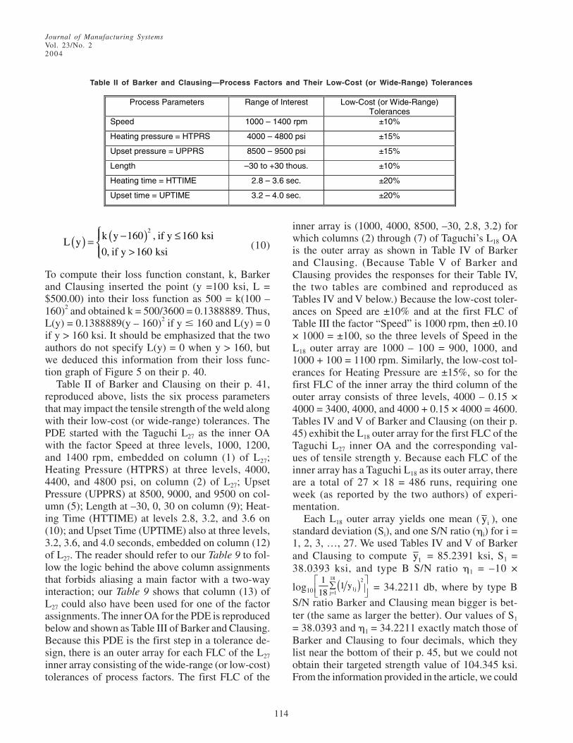
Journal of Manufacturing SystemsVol. 23/No. 22004
114
L yk y if y ksi
if y ksi( ) = −( ) ≤
>
⎧⎨⎪
⎩⎪160 160
0 160
2,
,(10)
To compute their loss function constant, k, Barkerand Clausing inserted the point (y =100 ksi, L =$500.00) into their loss function as 500 = k(100 –160)2 and obtained k = 500/3600 = 0.1388889. Thus,L(y) = 0.1388889(y – 160)2 if y � 160 and L(y) = 0if y > 160 ksi. It should be emphasized that the twoauthors do not specify L(y) = 0 when y > 160, butwe deduced this information from their loss func-tion graph of Figure 5 on their p. 40.
Table II of Barker and Clausing on their p. 41,reproduced above, lists the six process parametersthat may impact the tensile strength of the weld alongwith their low-cost (or wide-range) tolerances. ThePDE started with the Taguchi L27 as the inner OAwith the factor Speed at three levels, 1000, 1200,and 1400 rpm, embedded on column (1) of L27;Heating Pressure (HTPRS) at three levels, 4000,4400, and 4800 psi, on column (2) of L27; UpsetPressure (UPPRS) at 8500, 9000, and 9500 on col-umn (5); Length at –30, 0, 30 on column (9); Heat-ing Time (HTTIME) at levels 2.8, 3.2, and 3.6 on(10); and Upset Time (UPTIME) also at three levels,3.2, 3.6, and 4.0 seconds, embedded on column (12)of L27. The reader should refer to our Table 9 to fol-low the logic behind the above column assignmentsthat forbids aliasing a main factor with a two-wayinteraction; our Table 9 shows that column (13) ofL27 could also have been used for one of the factorassignments. The inner OA for the PDE is reproducedbelow and shown as Table III of Barker and Clausing.Because this PDE is the first step in a tolerance de-sign, there is an outer array for each FLC of the L27
inner array consisting of the wide-range (or low-cost)tolerances of process factors. The first FLC of the
inner array is (1000, 4000, 8500, –30, 2.8, 3.2) forwhich columns (2) through (7) of Taguchi’s L18 OAis the outer array as shown in Table IV of Barkerand Clausing. (Because Table V of Barker andClausing provides the responses for their Table IV,the two tables are combined and reproduced asTables IV and V below.) Because the low-cost toler-ances on Speed are ±10% and at the first FLC ofTable III the factor “Speed” is 1000 rpm, then ±0.10× 1000 = ±100, so the three levels of Speed in theL18 outer array are 1000 – 100 = 900, 1000, and1000 + 100 = 1100 rpm. Similarly, the low-cost tol-erances for Heating Pressure are ±15%, so for thefirst FLC of the inner array the third column of theouter array consists of three levels, 4000 – 0.15 ×4000 = 3400, 4000, and 4000 + 0.15 × 4000 = 4600.Tables IV and V of Barker and Clausing (on their p.45) exhibit the L18 outer array for the first FLC of theTaguchi L27 inner OA and the corresponding val-ues of tensile strength y. Because each FLC of theinner array has a Taguchi L18 as its outer array, thereare a total of 27 × 18 = 486 runs, requiring oneweek (as reported by the two authors) of experi-mentation.
Each L18 outer array yields one mean ( iy ), onestandard deviation (Si), and one S/N ratio (�i) for i =1, 2, 3, …, 27. We used Tables IV and V of Barkerand Clausing to compute 1y = 85.2391 ksi, S1 =38.0393 ksi, and type B S/N ratio �1 = –10 ×
log10 ( )18 2
1jj 1
11 y
18 =
⎡ ⎤∑⎢ ⎥⎣ ⎦ = 34.2211 db, where by type B
S/N ratio Barker and Clausing mean bigger is bet-ter (the same as larger the better). Our values of S1
= 38.0393 and �1 = 34.2211 exactly match those ofBarker and Clausing to four decimals, which theylist near the bottom of their p. 45, but we could notobtain their targeted strength value of 104.345 ksi.From the information provided in the article, we could
Table II of Barker and Clausing—Process Factors and Their Low-Cost (or Wide-Range) Tolerances
Process Parameters Range of Interest Low-Cost (or Wide-Range) Tolerances
Speed 1000 – 1400 rpm ±10%
Heating pressure = HTPRS 4000 – 4800 psi ±15%
Upset pressure = UPPRS 8500 – 9500 psi ±15%
Length –30 to +30 thous. ±10%
Heating time = HTTIME 2.8 – 3.6 sec. ±20%
Upset time = UPTIME 3.2 – 4.0 sec. ±20%

Journal of Manufacturing SystemsVol. 23/No. 2
2004
115
not ascertain how the authors determined that thenominal (or targeted) value of tensile strength forthe FLC #1 was 104.345 while the realized experi-mental value of the mean computed from their TablesIV and V was 1y = 85.2391 ksi. Our concern here isthe fact that the targeted signal value of 104.345,although not achieved experimentally, was also usedalong with 26 other presumably nominal strengthvalues in their Table VI on their p. 46 to perform ananalysis of variance to identify the Signal factors.Because the raw data for the remaining 26 outer ar-rays of FLCs 2 through 27 of L27 were not provided,we are not presently sure how to interpret the strength
values provided by Barker and Clausing in their TableVI, which is also reproduced below. Further, Barkerand Clausing also provide the type N (nominal thebest) S/N ratio near the bottom of their p. 45 as �1 =8.76478, which they obtained from �1 = 10 ×
log10 ( )2
1 1y S⎡ ⎤⎣ ⎦ by using the nominal value of 104.345
for their 1y , while as mentioned above, the samplemean for the L18 outer array of FLC 1 is 1y =85.2391. If we use the realized value of 1y = 85.2391in our NTB type S/N ratio, we would obtain �1 = 10
× log10 ( )2y S 1 18⎡ ⎤−⎣ ⎦ = 6.95982.
Table III of Barker and Clausing—Taguchi’s L27 Used as Inner OA
Speed (1)
HTPRS (2)
UPPRS (5)
Length (9)
HTTIME (10)
UPTIME (12)
1000 4000 8500 –30 2.8 3.2
1000 4000 9000 0 3.2 3.6
1000 4000 9500 30 3.6 4.0
1000 4400 8500 0 3.2 4.0
1000 4400 9000 30 3.6 3.2
1000 4400 9500 –30 2.8 3.6
1000 4800 8500 30 3.6 3.6
1000 4800 9000 –30 2.8 4.0
1000 4800 9500 0 3.2 3.2
1200 4000 8500 0 3.6 3.6
1200 4000 9000 30 2.8 4.0
1200 4000 9500 –30 3.2 3.2
1200 4400 8500 30 2.8 3.2
1200 4400 9000 –30 3.2 3.6
1200 4400 9500 0 3.6 4.0
1200 4800 8500 –30 3.2 4.0
1200 4800 9000 0 3.6 3.2
1200 4800 9500 30 2.8 3.6
1400 4000 8500 30 3.2 4.0
1400 4000 9000 –30 3.6 3.2
1400 4000 9500 0 2.8 3.6
1400 4400 8500 –30 3.6 3.6
1400 4400 9000 0 2.8 4.0
1400 4400 9500 30 3.2 3.2
1400 4800 8500 0 2.8 3.2
1400 4800 9000 30 3.2 3.6
1400 4800 9500 –30 3.6 4.0

Journal of Manufacturing SystemsVol. 23/No. 22004
116
It should be noted that the authors did use the S/Nratios obtained from the experimental results to ob-tain their MSs (mean squares) in their Table VII forS/N, but as far as we could ascertain they used thetargeted strength values to obtain their MSs for thestrength values. We could not resolve this trouble-some issue from all the data that were provided intheir article. To explain the values in Table VII ofBarker and Clausing, we are providing RTs for bothS/N ratio and Strength in our Tables 15 and 16, re-spectively. In Table 15, one asterisk on an F statisticimplies significance at the 5% level and two aster-isks on an F implies statistical significance at the 1%level. Using the S/N ratios from Table VI of Barkerand Clausing, the SS(Total�) = USS� – CF� =34935.110 – 33376.685 = 1558.4252 →SS(Residual�) = 345.5563 → MS(RES�) = 345.5563/14 = 24.683, which differs a bit from Barker andClausing’s MSRES = 26.00 in their Table VII (p. 46).The discrepancy could be due to the fact that theauthors provide only one-decimal accuracy in theirTable VI for both S/N and Strength values. In our Table
15, we obtained the linear and quadratic contrasts forthe six factors by applying the orthogonal polyno-mial coefficients PL = −[ ]′1 0 1 and PQ = 1 2 1−[ ]′ .Note that these two 3-D vectors are contrasts (that is,the components of PL and PQ add to zero) and theyare perpendicular (or orthogonal) because their vec-tor dot product is zero. In our Table 15, the linearcontrast for speed was computed from SpeedL = –1× 298.4 + 0 × 334.2 + 1 × 306.7 = 8.3, and the qua-dratic contrast was computed from SpeedQ = 1 ×298.4 – 2 × 334.2 + 1 × 306.7 = –83.3 (concavedownward). Because the factor “Speed” is at threelevels with 2 df, each of these two contrasts carryexactly 1 df, and thus the SS and MS of contrasts arethe same, while the MS(Speed) = SS(Speed)/2. TheSS of these two contrasts were computed from
SS(SpeedL) = 28.3
2 9× and SS(SpeedQ) = ( )2
83.3
6 9
−×
. Fur-
ther, few of the MSs that Barker and Clausing pro-vide in their Table VII are actually the SS as shownin Table 15. To check our answers, we ran Minitab’sGLM (general linear model) on the S/N ratio of the
Tables IV and V of Barker and Clausing—Using Taguchi’s L18 as Outer Array for First FLC ofTaguchi’s L27 Inner Orthogonal Array
Speed (2)
HTPRS (3)
UPPRS (4)
Length (5)
HTTIME (6)
UPTIME (7)
Tensile Strength (y)
900 3400 7225 –27 2.24 2.56 26.7038
900 4000 8500 –30 2.8 3.2 90.9161
900 4600 9775 –33 3.36 3.84 133.1830
1000 3400 7225 –30 2.8 3.84 84.7627
1000 4000 8500 –33 3.36 2.56 40.8376
1000 4600 9775 –27 2.24 3.2 120.489
1100 3400 8500 –27 3.36 3.2 94.7072
1100 4000 9775 –30 2.24 3.84 146.1440
1100 4600 7225 –33 2.8 2.56 29.4095
900 3400 9775 –33 2.8 3.2 111.1420
900 4000 7225 –27 3.36 3.84 72.2078
900 4600 8500 –30 2.24 2.56 22.4529
1000 3400 8500 –33 2.24 3.84 124.7730
1000 4000 9775 –27 2.8 2.56 72.4566
1000 4600 7225 –30 3.36 3.2 93.8594
1100 3400 9775 –30 3.36 2.56 58.6379
1100 4000 7225 –33 2.24 3.2 88.8731
1100 4600 8500 –27 2.8 3.84 122.7480

Journal of Manufacturing SystemsVol. 23/No. 2
2004
117
Table VI of Barker and Clausing—Using Taguchi’s L27 as Inner Array
Table VII of Barker and Clausing—ANOVA for S/N and Strength
Speed HTPRS UPPRS Length HTTIM UPTIME S/N STRENGTH STD. DEV.
1000 4000 8500 –30 2.8 3.2 34.2 104.3 38.04
1000 4000 9000 0 3.2 3.6 39.9 135.1 27.89
1000 4000 9500 30 3.6 4 12.3 128.6 45.16
1000 4400 8500 0 3.2 4 25.6 123.8 42.41
1000 4400 9000 30 3.6 3.2 37.5 134.6 45.59
1000 4400 9500 –30 2.8 3.6 40 134.7 27.06
1000 4800 8500 30 3.6 3.6 40.6 150.6 38.88
1000 4800 9000 –30 2.8 4 28.6 116.2 43.24
1000 4800 9500 0 3.2 3.2 39.7 151.2 45.03
1200 4000 8500 0 3.6 3.6 39.6 134.2 31.73
1200 4000 9000 30 2.8 4 35.4 134.1 41.28
1200 4000 9500 –30 3.2 3.2 39.1 132 40.67
1200 4400 8500 30 2.8 3.2 37.9 125.8 38.47
1200 4400 9000 –30 3.2 3.6 40.5 140.9 28.67
1200 4400 9500 0 3.6 4 37.8 158.5 46.85
1200 4800 8500 –30 3.2 4 30.9 129.6 44.86
1200 4800 9000 0 3.6 3.2 41.3 164.5 50.00
1200 4800 9500 30 2.8 3.6 41.7 156.1 29.91
1400 4000 8500 30 3.2 4 12.5 111.7 43.96
1400 4000 9000 –30 3.6 3.2 31.1 109.6 40.74
1400 4000 9500 0 2.8 3.6 40.8 146.7 30.66
1400 4400 8500 –30 3.6 3.6 38.3 125.6 37.59
1400 4400 9000 0 2.8 4 34.6 128.3 44.40
1400 4400 9500 30 3.2 3.2 39.3 139.1 44.84
1400 4800 8500 0 2.8 3.2 35.2 119.9 44.07
1400 4800 9000 30 3.2 3.6 40.8 148 36.84
1400 4800 9500 –30 3.6 4 34.1 150.1 53.13
S/N: Source MS F0 Strength: Source MS F0
Speedq 128.7 4.9 Speed 693 15.8
HTPRSL 126.8 4.8 HTPRS 1248 28.5
UPPRS 78 3.0 UPPRS 1633 37.3
Length 75 2.9 LengthL 407 9.3
HTTIME 25 1.0 Lengthq 434 9.9
UPTIMEL 388 14.9 HTTIME 452 10.3
UPTIMEq 350 13.5 UPTIME 611 14.0
Residual 26 Residual 44
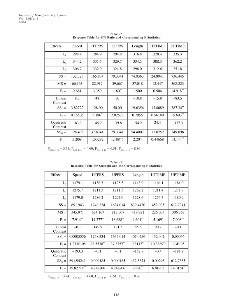
Journal of Manufacturing SystemsVol. 23/No. 22004
118
Table 15Response Table for S/N Ratio and Corresponding F Statistics
F0.05; 2, 14
= 3.74; F0.05; 1, 14
= 4.60; F0.01; 2, 14
= 6.51; F0.01; 1, 14
= 8.86
F0.05; 2, 14
= 3.74; F0.05; 1, 14
= 4.60; F0.01; 2, 14
= 6.51; F0.01; 1, 14
= 8.86
Table 16Response Table for Strength and the Corresponding F Statistics
Effects Speed HTPRS UPPRS Length HTTIME UPTIME
L1 298.4 284.9 294.8 316.8 328.4 335.3
L2 344.2 331.5 329.7 334.5 308.3 362.2
L3 306.7 332.9 324.8 298.0 312.6 251.8
SS = 132.325 165.834 79.3341 74.0363 24.8941 736.445
MS = 66.163 82.917 39.667 37.018 12.447 368.223
F0 = 2.681 3.359 1.607 1.500 0.504 14.918**
Linear Contrast
8.3 48 30 –18.8 –15.8 –83.5
SSL = 3.82722 128.00 50.00 19.6356 13.8689 387.347
F0 = 0.15506 5.186* 2.02572 0.7955 0.56189 15.693**
Quadratic Contrast
−83.3 −45.2 −39.8 −54.2 24.4 −137.3
SSQ = 128.498 37.8341 29.3341 54.4007 11.0252 349.098
F0 = 5.206* 1.53282 1.18845 2.204 0.44668 14.144**
Effects Speed HTPRS UPPRS Length HTTIME UPTIME
L1 1179.1 1136.3 1125.5 1143.0 1166.1 1181.0
L2 1275.7 1211.3 1211.3 1262.2 1211.4 1271.9
L3 1179.0 1286.2 1297.0 1228.6 1256.3 1180.9
SS = 691.943 1248.334 1634.014 839.4430 452.005 612.7341
MS = 345.971 624.167 817.007 419.721 226.003 306.367
F0 = 7.914** 14.277** 18.688** 9.601** 5.169* 7.008**
Linear Contrast
–0.1 149.9 171.5 85.6 90.2 –0.1
SSL = 0.0005556 1248.334 1634.014 407.0756 452.002 0.00056
F0 = 1.271E-05 28.5538** 37.3757** 9.3113** 10.3389** 1.3E-05
Quadratic Contrast
–193.3 –0.1 –0.1 –152.8 –0.4 –181.9
SSQ = 691.94241 0.000185 0.000185 432.3674 0.00296 612.7335
F0 = 15.82718** 4.24E-06 4.24E-06 9.890** 6.8E-05 14.0154**

Journal of Manufacturing SystemsVol. 23/No. 2
2004
119
authors’ Table VI, whose output is given below, andMinitab’s GLM verified our answers of Table 15.The entries at the bottom of Tables 15 and 16 areinverse functions of Fisher’s F distribution at the cdfvalues of 0.95 and 0.99, respectively.
ANOVA: SN vs. Speed, HTPRS, UPPRS, Length,HTTIME, UPTIME
General Linear Model: SN versus Speed, HTPRS, ...
Factor Type Levels ValuesSpeed fixed 3 1000, 1200, 1400HTPRS fixed 3 4000, 4400, 4800UPPRS fixed 3 8500, 9000, 9500Length fixed 3 –30, 0, 30HTTIME fixed 3 2.8, 3.2, 3.6UPTIME fixed 3 3.2, 3.6, 4.0
Analysis of Variance for SN, Using Adjusted SS for Tests
Source DF Seq SS Adj SS Adj MS F PSpeed 2 132.33 132.33 66.16 2.68 0.103HTPRS 2 165.83 165.83 82.92 3.36 0.064UPPRS 2 79.33 79.33 39.67 1.61 0.235Length 2 74.04 74.04 37.02 1.50 0.257HTTIME 2 24.89 24.89 12.45 0.50 0.614UPTIME 2 736.45 736.45 368.22 14.92 0.000Error 14 345.56 345.56 24.68Total 26 1558.43
S = 4.96816 R-Sq = 77.83% R-Sq(adj) = 58.82%
The above Minitab output shows that the mostinfluential factor that impacts the S/N ratio of Strengthis Upset Time, while Heating Pressure is significantat the 0.064 level and Speed’s effect is significant atthe 10.3% level. Thus, the only factors that impactprocess variability in the order of their influence areUpset Time, Heating Pressure, and Speed. From ourRT 15, Speed is optimal at L2 = 1200 rpm, HeatingPressure attains maximum S/N ratio at either L2 =4400 psi or L3 = 4800 psi, and Upset Time is optimalat its middle level, L2 = 3.60 seconds. We will breakthe tie between L2 = 4400 psi and L3 = 4800 psi ofHeating Pressure from the RT of Strength. The RTfor Strength values of Barker and Clausing’s TableVI is given in Table 16, and the associated Minitabfile, which also verified our answers, is available onrequest. Table 16 clearly shows that the impact ofUpset Pressure and Length are highly significant onthe mean Strength, while the effect of Heating Timeis statistically significant at the 5% level (F0 = 5.169> F0.05; 2, 14 = 3.74). Thus, these three process param-eters (UPPRS, Length, and HTTIME) are Signal fac-tors because they significantly influence the meanresponse but have minimal impact on variability ofy. Table 16 further shows that the optimal levels of
these Signal factors to maximize Strength areUPPRS3(L3 = 9500 psi), Length2(L2 = 0), andHTTIME3(L3 = 3.60 seconds). Further, we had achoice of two levels for the Control factor HTPRS(L2 = 4400 psi or L3 = 4800 psi). Because HeatingPressure has the maximum signal at 4800 psi, itsoptimal level is L3 = 4800 psi. Therefore, our opti-mum settings from our PDE for low-cost tolerancesare XO = Speed1200 HTPRS4800 UPPRS9500 Length0
HTTIME3.6 UPTIME3.6.The article by Barker and Clausing (1984) then
proceeded with a confirmation experiment at theabove optimum condition XO as a tolerance designwith low-cost tolerances, and the result is given intheir Table IX and reproduced below. The value ofthe mean for the confirmation run of Table IX is CNy= 159.7312 and the larger-the-better S/N ratio is �CN
= –10 × log10(MSD) = 43.2496, and the confirma-tion standard deviation SCN = 40.1526. Our values ofmean, S/N, and standard deviation match those ofthe authors listed near the bottom of their p. 49, butagain we could not determine how Barker andClausing arrived at their nominal strength value of184.152 for the confirmation experiment. The readershould observe that the optimal levels from the PDEhave improved the mean strength to CNy = 159.7312(barely below 160 ksi) but better than 26 out of the27 means listed in their original design Table VI.However, the variability measured by SCN = 40.1526is still too large (coefficient of variation is still morethan 25%), yielding a quality loss based only onvariability as L = kS2 = 0.138889 × 40.15262 =$223.921, which is consistent with the authors’ valueof $224 listed in their Table IX (p. 49). We have aslight problem with using k = 0.138889 for the lossfunction L = kS2 because the value of 0.138889 wascomputed for a modified form of the NTB loss func-tion given in Eq. (10). Because Strength is LTB, weused the Taguchi LTB loss function L(y) = k/y2 tocompute the constant k using the point (100 ksi, $500),which yields k = 5,000,000. Then, L = k(MSD) = 5 ×
106 ( )18 2
ii 1
11 y
18 =
⎡ ⎤∑⎢ ⎥⎣ ⎦ = 5 × 10⁶(0.00004732) = $236.5961,
which is in slight disagreement with the value of $224reported near the bottom of the authors’ p. 49.
Barker and Clausing (1984) next ran an ANOVAon the 18 strength values of their Table IX and pro-vided their results in Table X, which is reproducedbelow. There is a slight problem with Barker and

Journal of Manufacturing SystemsVol. 23/No. 22004
120
Source Sum of Squares (SS) % Contribution
Speed 772 2.0%
Heat pressure 9318 34.0%
Upset pressure 5595 20.0%
Length 535 2.0%
Heat time 5733 21.0%
Upset time 3312 12.0%
Residual No value was provided 9.0%
Table X of Barker and Clausing—Analysis of Sources of Variation
Table IX of Barker and Clausing—Confirmation Run at X0 with Wide-Range Tolerances
Speed: 1200±10%; HTPRS: 4800±15%; UPPRS: 9500±15%; Length: 0± 10%; HTTIME: 3.6±20%; UPTIME: 3.6±20%
Clausing’s Table X, which represents the ANOVAoutput from their Table IX design matrix. That is, intheir Table IX, the level of Length stays at zerothroughout the matrix and thus no SS (sum of squares)attributed to Length can be computed because levelsof Length have to change at least once before a SScan be computed. Our Minitab output with Length atzero at all 18 FLCs is provided below.
General Linear Model: Strength vs. Speed,HTPRS, ...
Factor Type Levels ValuesSpeed fixed 3 1080, 1200, 1320HTPRS fixed 3 4080, 4800, 5520UPPRS fixed 3 8075, 9500,10925HTTIME fixed 3 2.88, 3.60, 4.32UPTIME fixed 3 2.88, 3.60, 4.32
Speed (2)
HTPRS (3)
UPPRS (4)
Length (5)
HTTIME (6)
UPTIME (7)
Strength (y)
1080 4080 8075 0 2.88 2.88 93.8254
1080 4800 9500 0 3.6 3.6 180.285
1080 5520 10925 0 4.32 4.32 247.502
1200 4080 8075 0 3.6 4.32 96.4075
1200 4800 9500 0 4.32 2.88 173.245
1200 5520 10925 0 2.88 3.6 194.133
1320 4080 9500 0 4.32 3.6 151.143
1320 4800 10925 0 2.88 4.32 152.789
1320 5520 8075 0 3.6 2.88 148.251
1080 4080 10925 0 3.6 3.6 179.554
1080 4800 8075 0 4.32 4.32 142.253
1080 5520 9500 0 2.88 2.88 130.376
1200 4080 9500 0 2.88 4.32 124.819
1200 4800 10925 0 3.6 2.88 178.513
1200 5520 8075 0 4.32 3.6 229.883
1320 4080 10925 0 4.32 2.88 145.504
1320 4800 8075 0 2.88 3.6 131.302
1320 5520 9500 0 3.6 4.32 175.376

Journal of Manufacturing SystemsVol. 23/No. 2
2004
121
Analysis of Variance for Strength, Using Adjusted SS
for Tests
Source DF Seq SS Adj SS Adj MS F PSpeed 2 774.5 774.5 387.2 1.01 0.411HTPRS 2 9311.3 9311.3 4655.6 12.17 0.005UPPRS 2 5598.4 5598.4 2799.2 7.32 0.019HTTIME 2 5732.8 5732.8 2866.4 7.49 0.018UPTIME 2 3313.0 3313.0 1656.5 4.33 0.060Error 7 2678.0 2678.0 382.6Total 17 27407.9
S = 19.5594 = (382.6)1/2 R-Sq = 90.23% R-Sq(adj) = 76.27%
The only way that we could generate a SS for Lengthwas to replace the zeros in column (5) of Barker andClausing’s design matrix IX on their p. 49 with col-umn (5) of the Taguchi L18 OA, which is
[ ]1 2 3 2 3 1 1 2 3 3 1 2 3 1 2 2 3 1 ′
We again ran Minitab on the resulting design matrixand obtained the following output.
General Linear Model: Strength vs. Speed,HTPRS, ...
Factor Type Levels ValuesSpeed fixed 3 1080, 1200, 1320HTPRS fixed 3 4080, 4800, 5520UPPRS fixed 3 8075, 9500,10925Length fixed 3 1, 2, 3HTTIME fixed 3 2.88, 3.60, 4.32UPTIME fixed 3 2.88, 3.60, 4.32
Analysis of Variance for Strength, Using Adjusted SS
for TestsSource DF Seq SS Adj SS Adj MS F P %Contrib.Speed 2 774.5 774.5 387.2 0.90 0.462 2.826%HTPRS 2 9311.3 9311.3 4655.6 10.87 0.015 33.973%UPPRS 2 5598.4 5598.4 2799.2 6.53 0.040 20.426%Length 2 535.6 535.6 267.8 0.62 0.572 1.954%HTTIME 2 5732.8 5732.8 2866.4 6.69 0.039 20.917%UPTIME 2 3313.0 3313.0 1656.5 3.87 0.097 12.088%Error 5 2142.4 2142.4 428.5 7.816%Total 17 27407.9
S = 20.6998 R-Sq = 92.18% R-Sq(adj) = 73.42%
Note that Minitab’s GLM does not provide a percentcontribution column, and as a result we usedMicrosoft Excel to compute the last column of theabove output. Further, the last column of the aboveMinitab output is in good agreement with Table X ofBarker and Clausing.
As stated earlier, although the mean strength hasimproved to CNy = 159.7312, variability for low-cost tolerances measured by standard deviation SCN
= 40.1526 is still too large, causing 10 out of the 18confirmation runs to have strength values well be-low 160 ksi. The only option left for further vari-ance reduction is to find high-cost (or narrow-range)tolerances for the six process factors to reduce stan-
dard deviation from SCN = 40.1526 to a desired valueof, say Sd = 20 ksi, where the desired value of Sd =20 was selected by the authors. Thus, the desiredvariance of high-cost (or narrow-range) tolerancesis 2
dS = 400 ksi2, resulting in 400/40.15262 = 0.2481,or simply 24.81% of the low-cost variance of40.15262 = 1612.2313. To determine the high-costtolerances of the six factors, Barker and Clausingset up a tolerance reduction formula based on thepercent contribution of their Table X. Their trade-off tolerance reduction formula, based on Table X,is duplicated below and designated as Eq. (11).
( )
( )
2 2
2
2 22
Speed HTPRS UPPRS
1 10.2481 1 0.02 0.34 0.20
hp up
Length HTTIME UPTIME Residual
1 11 0.02 0.21 0.12 0.09
ht ut
⎛ ⎞ ⎛ ⎞= + × + × +⎜ ⎟ ⎜ ⎟
⎝ ⎠ ⎝ ⎠
⎛ ⎞ ⎛ ⎞+ × + × +⎜ ⎟ ⎜ ⎟⎝ ⎠ ⎝ ⎠
As Barker and Clausing state on their p. 48, Speedand Length had minimal impact on variation(roughly a total of 4%) and thus it is not worthwhiletightening their tolerances. As a result, they kept theSpeed and Length tolerances at the low cost of ±10%.The authors’ tolerance reduction Eq. (11) has an in-finite number of solutions for hp, up, ht, and ut toreach a goal of 24.81%. Although there are an infi-nite number of solutions to the rational tolerance re-duction Eq. (11), in practice the values of hp, up, ht,and ut should be determined not only to reach thedesired goal of 0.2481 but also to minimize the costof tolerance reduction. One possible solution thatBarker and Clausing (1984) provide at the bottomof their p. 50 is to reduce the low-cost tolerances±15% of Heating Pressure by a factor of hp = 3 tohigh-cost tolerances ±5%; to reduce the low-cost tol-erances ±15% of Upset Pressure by a factor of up =2 to the high-cost tolerances ±7.5%; to reduce thelow-cost tolerances Heating Time by a factor of ht =4 from ±20% to ±5%; and to reduce the low-costtolerances of Upset Time by a factor of ut = 4 from±20% to ±5%. We inserted these values of hp = 3, up= 2, ht = 4, and ut = 4 into Eq. (11), and the left-handside of the Eq. (11) becomes 0.2384 so that the re-sulting variance reduction is a bit more than the de-sired amount of 0.2481. Another possible solution,out of infinite, is hp = 2.5, up = 3, ht = 3, and ut =
(11)

Journal of Manufacturing SystemsVol. 23/No. 22004
122
2.57, for which the left-hand side of Eq. (11) be-comes 0.2481.
Before presenting the authors’ Final Design Sec-tion, we must present an excellent quote from Barkerand Clausing (1984) from their p. 51, which is re-produced below:
“Based on the rational reduction of variation we setup a final design to verify our new tolerances. Weuse another 18 treatment Taguchi L18 OA and theresults show that the variation has been reduced aspredicted to a much more tolerable level. The S/Nis now 45 db which is 2.13 times better than the
Table XI of Barker and Clausing—Confirmation Experiment at XO Using High-Cost orTight-Range Tolerances Embedded in the Taguchi L18 OA
START END
Speed Wide Range 10% Tolerances 1200 rpm 10% Tolerances
HTPRS Wide Range 15% Tolerances 4800 psi 5% Tolerances (1/3 of original)
UPPRS Wide Range 15% Tolerances 9500 psi 7.5% Tolerances (cut in half)
Length Wide Range 10% Tolerances Zero 10% Tolerances
HTTIME Wide Range 20% Tolerances 3.6 sec. 5% Tolerances (1/4 of original)
UPTIME Wide Range 20% Tolerances 3.6 sec. 5% Tolerances (1/4 of original)
Strength Wide Range causing a big loss
Response LOSS: $350/engine
Strength Reduced range
Loss reduced LOSS: $22/engine
Table XII of Barker and Clausing—Summary of Experimental Work
Speed (2)
HTPRS (3)
UPPRS (4)
Length (5)
HTTIME (6)
UPTIME (7)
Strength (y)
1080 4440 8787.5 0 3.42 3.42 148.175
1080 4800 9500 0 3.6 3.6 180.285
1080 5160 10212.5 0 3.78 3.78 214.085
1200 4440 8787.5 0 3.6 3.78 154.614
1200 4800 9500 0 3.78 3.42 187.569
1200 5160 10212.5 0 3.42 3.6 203.285
1320 4440 9500 0 3.78 3.6 168.928
1320 4800 10212.5 0 3.42 3.78 186.335
1320 5160 8787.5 0 3.6 3.42 178.602
1080 4440 10212.5 0 3.6 3.6 179.920
1080 4800 8787.5 0 3.78 3.78 170.139
1080 5160 9500 0 3.42 3.42 183.808
1200 4440 9500 0 3.42 3.78 165.605
1200 4800 10212.5 0 3.6 3.42 195.667
1200 5160 8787.5 0 3.78 3.6 192.875
1320 4440 10212.5 0 3.78 3.42 180.443
1320 4800 8787.5 0 3.42 3.6 161.258
1320 5160 9500 0 3.6 3.78 192.165

Journal of Manufacturing SystemsVol. 23/No. 2
2004
123
best combination of our original design and far bet-ter than anything we would have achieved by trialand error. More importantly, we have come to alogical end point. There is no more searching forthat ‘pot of gold’ at the end of the rainbow thatoften goes on in a nonsystematic searches for opti-mum conditions.”
There may be a minor typographical error in theirS/N assessment in the above quote because we couldnot verify the value “2.13 times better” because thebest S/N ratio in the original design occurs at runnumber 18, whose S/N is �18 = 41.7 db.
As stated in the above quote, Barker and Clausing(1984) then conducted another set of confirmationexperiments at the optimal condition XO = Speed1200
HTPRS4800 UPPRS9500 Length0 HTTIME3.6 UPTIME3.6
with high-cost tolerances Speed: 1200 ± 10%,HTPRS: 4800 ± 5%, UPPRS: 9500 ± 7.5%, Length:0 ± 10%, HTTIME: 3.6 ± 5%, and UPTIME: 3.6 ±5% using a Taguchi L18 OA. The results are given intheir Table XI (p. 51) and duplicated above. TableXI of Barker and Clausing may have a minor errorbecause the high-cost (or tight-range) tolerances ofHeating Pressure are 4800 ± 5% = 4800 – 0.05 ×4800, 4800, 4800 + 0.05 × 4800 = 4560, 4800, 5040,while they are listing 4440, 4800, and 5160 as thethree levels of HTPRS in their L18 outer OA. We donot know if this minor error is typographical or if4440, 4800, and 5160 are the actual levels used inthe final tolerance design confirmation runs. If in-deed the HTPRS levels were set at 4440, 4800, and5160, then the high-cost tolerances that are beingused for HTPRS are 4800 ± 7.5% (not the requiredamount of ±5%), so the actual value of hp = 2 andnot the required amount of 3. With hp = 2, up = 2, ht= 4, and ut = 4, the LHS of Eq. (11) becomes 0.2856(not satisfying the desired amount of 0.2481).
We computed the mean, standard deviation, andthe larger-the-better S/N ratio of Table XI of Barkerand Clausing (1984), obtaining XIy = 180.2088, SXI
= 16.8246, and �XI = 45.00522, which are identical tothose of the authors’ to three-decimal accuracy, whichthey list near the bottom of their p. 51. The authorsthen state that the amount of QLs has been reduced to$22/engine in their Table XII, which is reproducedabove. We tried to use the data of Table XI of Barkerand Clausing to reproduce the amount of reduced QLsthat Barker and Clausing report as $22/engine at thebottom of their Table XII. We attempted three differ-
ent methods to obtain the average quality loss/engineof $22, which are summarized below.
1. L = k × 2XIS = 0.138889 × 16.82462 = 39.3149
(not too far from $22/engine)
2a. L = k × MSD, where MSD = ( )18 2
ii 1
11 y
18 =∑ =
0.000568526/18 = 0.0000315848 Æ L =5000000 × 0.0000315848 = $157.924 (veryfar from the stated $22/engine)
2b. Or, since �db = –10 × log10(MSD), L = k ×(10–�db/10) = 5000000 × (10–4.500522) = $157.924(identical to 2(a) as expected)
3. Using the modified loss function L(y) =
( )2k y 160 , if y 160 ksi
0, if y 160 ksi
⎧⎪ − ≤⎨
>⎪⎩ , we obtained (see Table
XI of Barker and Clausing) L = k × [(148.175– 160)2 + (154.614 – 160)2]/18 = 0.138889 ×[(–11.825)2 + (–5.386)2]/18 = $1.3028 (notclose to $22/engine)
Presently, we are not sure how Barker andClausing arrived at their L = $22/engine. However,it is quite clear that Taguchi’s tolerance design hasled to a tremendous amount of reduction in societalQLs. Even if we take the average of the above threedistinct computed quality losses, we obtain an L =(39.3149 + 157.924 + 1.3028)/3 = $66.1806, whichis a quality loss reduction of ($350 – $66.1806)/$350= 81.09% (a remarkable achievement).
14. Summary and ConclusionsIn this article, each of Taguchi’s major contribu-
tions has been presented and described in sufficientdetail to allow the reader to understand and use thetools presented. Taguchi’s contributions were iden-tified as:
• The quantification of quality through Gauss’sQuality Loss Function*
• Orthogonal Arrays to simplify the use of De-sign of Experiments (DOE)
• Robust Designs (Parameter and ToleranceDesigns) to identify optimum settings to re-duce process variability and to get the meanon target*
• Definition and use of the Signal-to-Noise (S/N)Ratio, which combines the mean and standarddeviation into one measure

Journal of Manufacturing SystemsVol. 23/No. 22004
124
where * implies Taguchi’s major contributions. Eachof the above contributions was reviewed in detailwith an objective review of accolades and criticismsof each contribution and examples of its use.
The Quality Loss Function was introduced as oneof Taguchi’s two greatest contributions. By apply-ing Gauss’s quadratic loss, Taguchi was able to quan-tify quality as deviation from the ideal target (insteadof the traditional view that cost is incurred only whenresults do not meet design or consumer specifica-tions). This contribution of Taguchi induced a changein philosophy by manufacturers, who now realizethat to minimize total cost they must reduce vari-ability around a customer-defined target instead ofjust meeting customer specifications.
Although Orthogonal Arrays (OAs) were not “in-vented” by Dr. Taguchi (many are actually classical(fractional) factorial designs credited to Sir R.A.Fisher, Box and Hunter, Kempthorne, Yates, andother notables), he can certainly be credited withpopularizing their use by simplifying their format.This article explained how OAs are constructed, theimportance of their alias structure and design reso-lution, and provided examples of the constructionand use of some of the more popular Taguchi’s OAs,specifically the L8, L16, L27, and L18 designs. Thecontents presented herein can also aid those whowish to use the Taguchi and Konishi (1987) book onorthogonal arrays.
Taguchi’s Robust (Parameter and Tolerance) De-signs are the other most significant contributions;both were reviewed with examples of each. Param-eter Design Experiments use inner and outer OAs toidentify the Control and Signal factors through theuse of Signal-to-Noise Ratio (S/N). The optimum lev-els are identified with a resulting cost reduction (us-ing Taguchi’s Loss Function). The authors used anexample from Barker and Clausing (1984) to showhow Taguchi’s Parameter Design is used to identifyoptimum process condition, followed by ToleranceDesign to tighten factor tolerances to attain suffi-cient reduction in process variation. As a general rule,we would recommend to the process or manufactur-ing engineer to use a single classical FFD with maxi-mum resolution if the QCH of interest is STB or LTBand if the CV is known to be < 20%. However, if theQCH is a nominal dimension, then it is best to useTaguchi’s crossed-array (or inner and outer OAs) toperform DOE.
Throughout the discussions on Robust Designs,the Signal-to-Noise Ratio was used. This is perhapsone of Taguchi’s most controversial contributionsbecause some Western statisticians believe thatsample mean and variance should be analyzed sepa-rately since they are stochastically independent fora Gaussian process. The example used for Param-eter Design was also presented by analyzing the meanand variance separately (as compared to the analy-sis using S/N), and results were presented that werein slight disagreement with the results obtained fromthe use of the S/N ratio. The dilemma of when to useTaguchi’s S/N ratios and when to analyze the meanand ln(S) separately is an interesting problem thatshould be investigated in the future.
Finally, all manufacturing and process engineersshould be well aware of the fact that Sir Ronald A.Fisher is the founder of the field of DOE, and Dr.Taguchi is one of the pioneers of its applications toprocess and manufacturing engineering. Taguchi fa-cilitated the use of the very same methodology thatSir Fisher started in the early 1920s and on whichmany prominent Western 20th-century statisticianscontinued to expand and build.
Nomenclature
ANOVA Analysis of VarianceCV Coefficient of VariationCF Correction FactorCIs Confidence Intervalscdf Cumulative Distribution Functiondf Degrees of FreedomDOE Design of ExperimentsFF Fractional FactorialFFD Fractional Factorial DesignFLC Factor Level CombinationFNC Fraction NonconformingGLM General Linear Modelk Loss function coefficient and the num-
ber of factors in a factorial or FFDL Mean (or Average) Quality LossLHS Left Hand SideLTB Larger the BetterLSL Lower Specification LimitL(y) Quality Loss Function for a single itemmod ModulusMSD Mean Squared DeviationMS Mean Square

Journal of Manufacturing SystemsVol. 23/No. 2
2004
125
Nf Number of Distinct Factor Level com-binations
NTB Nominal the BestOA Orthogonal ArrayPCR Process Capability RatioPDE Parameter Design ExperimentPEC Present Existing ConditionQCH Quality CharacteristicQL Quality LossQLF Quality Loss FunctionQD Quality DifferenceQI Quality ImprovementR ResolutionRT Response TableRHS Right Hand SideS/N Signal to NoiseSS Sum of SquaresSTB Smaller the BetterSPC Statistical Process ControlTOIBTC Table of Interactions Between Two Col-
umnsUSL Upper Specification Limit
CNy Mean of Confirmation runs
BibliographyAmerican Supplier Institute (ASI), Inc. (1984). Seminar Series B.
Dearborn, MI: Center for Taguchi Methods.Antony, J. (1999). “How to analyze and interpret Taguchi experi-
ments.” Journal of Quality World (Feb. 1999), pp42-49.Barker, T.B. and Clausing, D.P. (1984). “Quality engineering by de-
sign, the Taguchi method.” 40th Annual RSQC Conf., March 1986.Barker, T.B. (1986). “Quality engineering by design: Taguchi’s phi-
losophy.” Quality Progress (v19, n12, Dec. 1986), pp32-42.Basso, L.; Winterbottom, A; and Wynn, H.P. (1986). “A review of the
‘Taguchi methods’ for off-line quality control.” Quality and Reli-ability Engg. (v2), pp71-79.
Bisgaard, S. (1990). “Quality engineering and Taguchi methods: aperspective.” CQPI Reports (n40). Madison, WI: Center for Qual-ity and Productivity Improvement, Univ. of Wisconsin.
Bisgaard, S. (1991). “Process optimization - going beyond Taguchimethods.” CQPI Reports (n70). Madison, WI: Center for Qualityand Productivity Improvement, Univ. of Wisconsin.
Bisgaard, S. (1992). “A comparative analysis of the performance ofTaguchi’s linear graphs.” CQPI Reports (n82). Madison, WI: Centerfor Quality and Productivity Improvement, Univ. of Wisconsin.
Bisgaard, S. and Diamond, N.T. (1990). “An analysis of Taguchi’smethod of confirmatory trials.” CQPI Reports (n60). Madison,WI: Center for Quality and Productivity Improvement, Univ. ofWisconsin.
Bisgaard, S. and Ankenman, B. (1993). “Analytic Parameter Design.”CQPI Reports (n103). Madison, WI: Center for Quality and Pro-ductivity Improvement, Univ. of Wisconsin.
Box, G.E.P. (1988). “Signal-to-noise ratios, performance criteria andtransformation.” Technometrics (v30, n1), pp1-17.
Box, G.E.P. and Fung, C.A. (1986). “Minimizing transmitted varia-tion by parameter design.” Report No. 8. Madison, WI: Center forQuality and Productivity Improvement of Univ. of Wisconsin.
Box, G.E.P.; Bisgaard, Soren; and Fung, Conrad (1988). “An expla-nation and critique of Taguchi’s contributions to quality engineer-ing.” Quality and Reliability Engg. Int’l (v4, n2), pp123-131.
Box, G.E.P. and Hunter, J.S. (1961a). “The 2k–p fractional factorialdesigns, part I.” Technometrics (v3, n3), pp311-351.
Box, G.E.P. and Hunter, J.S. (1961b). “The 2k–p fractional factorialdesigns, part II.” Technometrics (v3, n4), pp449-458.
Box, G.E.P. and Jones, S. (1992). “Designing products that are robustto the environment.” Total Quality Mgmt. (v3, n3), pp265-282.
Bulington, E.B.; Hool, J.N.; and Maghsoodloo, S. (1990). “A simplemethod for obtaining Resolution IV designs for use with Taguchi’sorthogonal arrays.” Journal of Quality Technology (v22, n4),pp260-264.
Byrne, D.M. and Taguchi, S. (1987). “The Taguchi approach to pa-rameter design.” Quality Progress (v20, n12), pp19-26.
Campanella, J. (1990). Principles of Quality Costs. Milwaukee, WI:ASQC Quality Press.
Chiu, Hsin-Cheng (1995). “Statistical tolerance limits.” MS thesis.Auburn, AL: Auburn Univ.
Conner, W.S. and Zelen, M. (1959). “Fractional factorial experimentdesigns for factors at three levels.” National Bureau of StandardsApplied Mathematics Series (n54).
Czitrom, V. (1990). “An application of Taguchi’s methods reconsid-ered.” Presented at ASA meeting, Washington, DC, 1989.
Cochran, W.G. and Cox, G.M. (1957). Experimental Designs, 2nd ed.New York: John Wiley & Sons.
Davies, O.L. et al. (1967). The Design and Analysis of Experiments.New York: Hafner Publishing Co.
Draper, N.R. and Hunter, W.G. (1969). “Transformations: some ex-amples revisited.” Technometrics (v11, n1), pp23-40.
Draper, N.R. and Mitchell, T.J. (1970). “Construction of a set of 512-run designs of resolution � 5 and a set of even 1024-run designsof resolution � 6.” Annals of Mathematical Statistics (v4, n3),pp876-887.
Ealey, L.A. (1988). Quality by Design: Taguchi Methods and U.S.Industry. Beachwood, OH: ASI Press.
Fisher, R.A. (1966). The Design of Experiments, 8th ed. New York:Hafner Publishing Co.
Fries, A. and Hunter, W.G. (1980). “Minimum aberration 2k–p de-signs.” Technometrics (v22, n4), pp601-608.
Graybill, F.A. (1961). An Introduction to Linear Statistical Models.New York: McGraw-Hill.
Hicks, C.R. and Turner, K.V., Jr. (1999). Fundamental Concepts inthe Design of Experiments, 5th ed. Oxford Univ. Press.
John, P.W.M. (1961). “The three-quarter replicates of 24 and 25 de-signs.” Biometrics (v17), pp319-321.
John, P.W.M. (1962). “Three-quarter replicates of 2n designs.” Bio-metrics (v18, n2), pp172-184.
John, P.W.M. (1964). “Blocking a 3(2n–k) design.” Technometrics (v6,n4), pp371-376.
Juran, J.M. and Godfrey, A.B., eds. (1999). Juran’s Quality Hand-book. New York: McGraw-Hill.
Kackar, R.N. and Phadke, M.S. (1984). “An introduction to off-linequality control methods.” Int’l QC Forum (v2, n8).
Kackar, R.N. (1985). “Off-line quality control, parameter design andthe Taguchi method.” Journal of Quality Technology (v17, n4),pp176-209.
Kackar, R.N. (1986). “Taguchi’s quality philosophy: analysis andcommentary.” Quality Progress (v19, n12), pp21-29.
Kackar, R.N. and Tsui, K-L. (1990). “Interaction graphs: graphicalaids for planning experiments.” Journal of Quality Technology(v22, n1), pp1-14.
Kapur, K.C. and Chen, G. (1988). “Signal-to-noise ratios develop-ment for quality engineering.” Quality and Reliability Engg. (v4,n2), pp133-141.
Kempthorne, O. (1952). The Design and Analysis of Experiments.New York: John Wiley & Sons.

Journal of Manufacturing SystemsVol. 23/No. 22004
126
Kim, Y.J. and Cho, B.R. (2000). “Economic considerations on pa-rameter design.” Quality and Reliability Engg. Int’l (v16, n6),pp501-514.
Leon, R.V.; Shoemaker, A.C.; and Kackar, R.N. (1987). “Perfor-mance measures independent of adjustment - an explanation andextension of Taguchi’s signal-to-noise ratios.” Technometrics (v29,n3), pp253-265.
Li, M.-H.C. (2000). “Quality loss function based manufacturing pro-cess setting models for unbalanced tolerance design.” Int’l Jour-nal of Advanced Mfg. Technology (v16, n1), pp39-45.
Lin, P.K.H.; Sullivan, L.P.; and Taguchi, G. (1990). “Using Taguchimethods in quality engineering.” Quality Progress (v23, n9),pp55-59.
Logothetis, N. and Wynn, H.P. (1989). Quality through Design: Ex-perimental Design, Off-line Quality Control, and Taguchi’s Con-tributions. New York: Oxford Science Publications.
Maghsoodloo, S. (1990). “The exact relation of Taguchi’s signal-to-noise ratio to his quality loss function.” Journal of Quality Tech-nology (v22, n1), pp57-67.
Maghsoodloo, S. (1992). Introduction to Taguchi-Based QualityDesign and Improvement. Auburn, AL: Auburn Univ., Engineer-ing Learning Resources, College of Engg.
Maghsoodloo, S. and Li, M-H.C. (2000). “Optimal asymmetric toler-ance design.” IIE Trans. (v32, n12), pp1127-1137.
Margolin, B.H. (1969). “Results on factorial designs of Resolution IVfor the 2n and 2n3m series.” Technometrics (v11, n3), pp431-444.
Montgomery, D.C. (1997). Design and Analysis of Experiments, 4thed. New York: John Wiley & Sons.
Montgomery, D.C. (2001a). Design and Analysis of Experiments, 5thed. New York: John Wiley & Sons.
Montgomery, D.C. (2001b). Introduction to Statistical Quality Con-trol, 4th ed. New York: John Wiley & Sons.
Montgomery, D.C. and Runger, G.C. (1996). “Foldovers of 2k–p Reso-lution IV designs.” Journal of Quality Technology (v28, n4),pp446-450.
Nair, V.N. (1992). “Taguchi’s parameter design.” Technometrics (v34,n2), pp128-161.
Peace, G.S. (1993). “Taguchi Methods: A Hands-On Approach.” Read-ing, MA: Addison-Wesley Publishing Co.
Pignatiello, J.J., Jr. and Ramberg, J.S. (1991-92). “Top ten triumphs andtragedies of Genichi Taguchi.” Quality Engg. (v4, n2), pp211-225.
Plackett, R.L. and Burman, J.P. (1946). “The design of optimummultifactor experiments.” Biometrika (v33), pp305-325.
Ribeiro, J.L.D. and Elsayed, E.A. (1995). “A case study on processoptimization using the gradient loss function.” Int’l Journal ofProduction Research (v33, n12), pp3233-3248.
Robinson, T.J.; Borror, C.M.; and Myers, R.H. (2004). “Robust pa-rameter design: a review.” Quality and Reliability Engg. Int’l(v20, n1), pp81-101.
Ross, P.J. (1988). “The role of Taguchi methods and design of experi-ments in QFD.” Quality Progress (v21, n6), pp41-47.
Ross, P.J. (1988). Taguchi Techniques for Quality Engineering. NewYork: McGraw-Hill.
Roy, R.K. (1990). A Primer on the Taguchi Method. New York: VanNostrand Reinhold.
Scheffé, H. (1953). “A method for judging all contrasts in the analy-sis of variance.” Biometrika (v40, n1/2), pp87-104.
Scheffé, H. (1956). “A ‘mixed model’ for the analysis of variance.”Annals of Mathematical Statistics (v27), pp23-36.
Scheffé, H. (1959). The Analysis of Variance. New York: John Wiley& Sons.
Searle, S.R. (1971a). Linear Models. New York: John Wiley & Sons.Searle, S.R. (1971b). “Topics in variance component estimation.”
Biometrics (v27, n1), pp1-76.Shoemaker, A.C. and Tsui, K-L. (1991). “Economical experimentation
methods for robust design.” Technometrics (v33, n4), pp415-427.Steinberg, D. and Burnsztyn, D. (1993). “Noise factors, dispersion
effects and robust design.” CQPI Reports (n107). Madison, WI:Center for Quality and Productivity Improvement of Univ. ofWisconsin.
Stephens, M.P. (1994). “Comparison of robustness of Taguchi’s meth-ods with classical ANOVA under conditions of homogeneous vari-ances.” Quality Engg. (v7, n1), pp147-168.
Sullivan, L.P. (1987). “The power of Taguchi methods.” QualityProgress (v20, n6), pp76-79.
Taguchi, G. (1986). Introduction to Quality Engineering: DesigningQuality into Products and Processes. Tokyo: Asian ProductivityOrganization.
Taguchi, G.; Elsayed, E.A.; and Hsiang, T.C. (1989). Quality Engi-neering in Production Systems. New York: McGraw-Hill.
Taguchi, G. and Konishi, S. (1987). Taguchi Methods, OrthogonalArrays and Linear Graphs, Tools for Quality Engineering. AllenPark, MI: ASI Press.
Taguchi, G. (1993a). Taguchi Methods, Design of Experiments. Qual-ity Engineering Series, Vol. 4. Dearborn, MI: Japanese StandardsAssociation and American Supplier Institute.
Taguchi, G. (1993b). Taguchi on Robust Technology Development:Bringing Quality Engineering Upstream. New York: ASME Press.
Tsui, K.-L. (1996). “A critical look at Taguchi’s modeling approach forrobust design.” Journal of Applied Statistics (v23, n1), pp81-95.
Tukey, J.W. (1949). “Comparing individual means in the analysis ofvariance.” Biometrics (v5, n2), pp99-114.
Webb, S. (1968). “Non-orthogonal designs of even resolution.”Technometrics (v10, n2), pp291-299.
Yates, F. (1937). The Design and Analysis of Factorial Experiments.Imperial Bureau of Soil Sciences (Harpenden).
Authors’ BiographiesDr. Saeed Maghsoodloo is a professor in the Dept. of Industrial
and Systems Engineering at Auburn University, Auburn, Alabama.His research interests and publications are in the areas of design ofexperiments, off-line and on-line quality control, multivariate analy-sis, regression/correlation and time-series analysis, reliability engi-neering, and nonparametric statistics. He is a member of ASA andASQ and is an associate editor of IIE Transactions and the Journal ofManufacturing Systems and is a reviewer for numerous national andinternational journals. He is a registered professional engineer in thestate of Alabama and is on the editorial board of Quality and Reliabil-ity Engineering of IIE Transactions.
Dr. Gultekin Ozdemir is an assistant professor in the Dept. ofIndustrial Engineering at Suleyman Demirel University, Turkey. Hereceived a BSc degree from Anadolu University (Turkey), MSc de-grees from West Virginia University and the University of Pittsburgh,and a PhD degree from Auburn University in industrial engineering.His research interests are in the areas of quality engineering, Taguchimethods, applied statistics, and heuristic optimization techniques suchas genetic algorithms.