2002-cc kr-elastoviscoplastic fe analysis in matlab
TRANSCRIPT

8/10/2019 2002-CC KR-Elastoviscoplastic FE Analysis in Matlab
http://slidepdf.com/reader/full/2002-cc-kr-elastoviscoplastic-fe-analysis-in-matlab 1/36
J. Numer. Math., Vol. 10, No. 3, pp. 157–192 (2002)
c VSP 2002
Elastoviscoplastic Finite Element analysisin 100 lines of Matlab
C. Carstensen and R. Klose †
Received 3 July, 2002
Abstract — This paper provides a short Matlab implementation with documentation of the P1 finiteelement method for the numerical solution of viscoplastic and elastoplastic evolution problems in 2Dand 3D for von-Mises yield functions and Prandtl-Reuß flow rules. The material behaviour includesperfect plasticity as well as isotropic and kinematic hardening with or without a viscoplastic penali-sation in a dual model, i.e. with displacements and the stresses as the main variables. The numericalrealisation, however, eliminates the internal variables and becomes displacement-oriented in the end.Any adaption from the given three time-depending examples to more complex applications can easilybe performed because of the shortness of the program and the given documentation. In the numerical2D and 3D examples an efficient error estimator is realized to monitor the stress error.
Keywords: finite element method, viscoplasticity, elastoplasticity, Matlab
1. INTRODUCTION
Elastoplastic time-evolution problems usually require universal, complex, commer-
cial computer codes running on workstations or even super computers [11,15]. The
argument of keeping commercial secrets hidden inside a black-box, leaves the typ-
ical user without any idea what exactly is going on behind the program’s user-
friendly surface. The difference between a mathematical and a numerical model
is fuzzy. Often, users do not care about nasty details such as quadrature rules orthe exact material laws realised. But sometimes it does matter whether a regu-
larised or penalised discrete model is solved, how the termination of an iterative
process is steered, and what post-processing led to both, equilibrium and admissi-
bility of the approximate stress field. In particular, if the solution process is part
of guaranteed error control, it is quite important to know if discrete equilibrium is
fulfilled exactly or not. Finally, the use of more than one black-box in a chain is
likely to be less efficient. In summary, to aim efficiency (e.g. by well-adapting au-
tomatic mesh-refinements) and reliability we have to prevent, at least confess, all Institute for Applied Mathematics and Numerical Analysis, Vienna University of Technology,
Wiedner Hauptstraße 8-10, A-1040 Vienna, Austria
†Mathematisches Seminar, Christian-Albrechts-Universitat zu Kiel, Ludewig-Meyn-Str. 4, D-24098 Kiel, Germany

8/10/2019 2002-CC KR-Elastoviscoplastic FE Analysis in Matlab
http://slidepdf.com/reader/full/2002-cc-kr-elastoviscoplastic-fe-analysis-in-matlab 2/36
158 C. Carstensen and R. Klose
the numerical crimes. Those range from modelling errors (e.g. data errors, coarse
geometrical resolution, wrong mathematical model, etc.) to variational crimes (e.g.
material laws fulfilled at discrete points only or just in some approximate sense).
This work aims a clear presentation of clean algorithms to compute a few model
examples. Their implementation in Matlab (as one possible higher scientific com-puting tool) is the content of this paper. The provided software may serve as both,
reference material for future numerical examples and as scientificly proved public
domain source for modifications in other applications for research and educational
purposes.
This paper continues our efforts on the Laplace and Navier–Lame problem [2,3]
towards more complicated material behaviour to advertise and to open the field of
computational plasticity to a larger community of applied mathematicians and engi-
neers. Within a small strain framework, the rheological models of this work includeperfect plasticity, elastoplastic evolution with kinematic or isotropic hardening in
the setting of von-Mises yield conditions and a Prandl-Reuß flow rule [11,15]. All
variants are available for a viscoplastic regularisation with a Yosida-regularisation,
known as viscoplasticity due to Perzyna.
The time discretisation yields a minimisation problem under severe constraints
for each time step. The discrete problem is solved with a Newton-Raphson scheme
and Matlab’s standard direct solver. The main principle of the presented method
is, that, in each time step, the stress tensor is expressed explicitly and applied in
Cauchy’s first law of motion.
We expect that the reader is familiar with Matlab as well as with linear elasticity
and otherwise refer, e.g. to [3,13].
The paper is organised as follows. In Section 2 we introduce the viscoplastic
and elastoplastic problem and their mathematical model. In Section 3 we perform a
time discretisation and calculate the explicit expression of the stress tensor for the
different models of hardening. In Section 4 the discretisation in space together with
the data representation of the triangulation, the Dirichlet and Neumann boundary is
considered. Furthermore the iterative solution of the discrete problem is explained.Section 5 concerns the calculation of the stiffness matrix. Section 6 discusses post
processing routines, one for previewing the numerical solution and one for an a
posteriori error estimation. Numerical examples in Section 7 illustrate the usage
of the provided tools for four benchmark examples in two and three space dimen-
sions.
The programs are written for Matlab 6.1 but adaption for previous versions ispossible. For a numerical calculation it is necessary to run the program
with (user-specified) files
,
,
, , as well as the subroutines , , and . Their meaning andusage is explained throughout the paper and examples are provided in the later sec-tions. The graphical representation is performed with the function and theerror is estimated in
. All files with the code and the data for allexamples can be downloaded from
.
8/10/2019 2002-CC KR-Elastoviscoplastic FE Analysis in Matlab
http://slidepdf.com/reader/full/2002-cc-kr-elastoviscoplastic-fe-analysis-in-matlab 3/36
Elastoviscoplastic FE analysis 159
2. RHEOLOGICAL MODEL
2.1. Material models
The material body occupies a bounded Lipschitz domainΩ
in
d
and deforms anytime t , 0 t T . Given a displacement field u u t H 1
Ω
d (i.e., the functionalmatrix Du exists almost everywhere in Ω, is measurable, and satisfies
Ω Du
2 d x
∞) the total strain reads
ε
u
Du
DuT
2
ε
u jk
u j
k
uk
j
2
j
k
1
d
In the engineering literature, ε u
is known as the linear Green strain tensor. Thedefault model for small-strain plasticity involves an additive split
ε ε ε
e
σ σ σ
p
ξξξ
of the total strain in an elastic part, e
σ σ σ
1σ σ σ , and an irreversible part p
ξξξ
.The plastic strain p
ξξξ
depends on further internal variables ξξξ . The stress field
σ σ σ
σ σ σ t L2
Ω;
d d sym
of the Cauchy stress tensor σ σ σ x t
is linked to the elas-
tic, reversible strain. The linear relation is provided by
1 , the compliance tensor,which is the inverse of the fourth order elasticity tensor
. In the numerical exam-ples, a two-parameter model (λ and µ are the Lame constants) in linear isotropic,homogeneous elasticity,
e
λ tr e I
2µ e, is employed.
The evolution law for the plastic strain p is more involved and requires theconcept of admissible stresses, a yield function, and an associated flow rule.The kinematic variables p and ξξξ form the generalised strain P
p
ξξξ
. The cor-responding generalised stress reads ΣΣΣ
σ σ σ α α α , where α α α
m
msym describes internal
stresses.We denote by K the set of admissible stresses, which is a closed, convex set,
containing 0, and is defined by
K
ΣΣΣ : Φ
ΣΣΣ
0
The yield function Φ describes admissible stresses by Φ ΣΣΣ 0 and models eitherperfect plasticity or hardening. The dissipation functional ϕ
ΣΣΣ
, defined by
ϕ σ σ σ α α α
1
2ν inf
σ σ σ τ τ τ α α α β β β
2 : τ τ τ β β β
d d sym
m msym
Φ τ τ τ β β β
0
(2.1)
approaches the indicator function of the set K, namely
ϕ
ΣΣΣ
0
Φ
ΣΣΣ
0
∞
Φ
ΣΣΣ
0(2.2)
as ν 0. The time derivative of P is given by the flow rule
P ∂ϕ ΣΣΣ σ σ σ α α α
d d sym
m msym :
τ τ τ β β β
d d sym
m msym
ϕ
σ σ σ
α α α
σ σ σ :
τ τ τ σ σ σ
α α α :
β β β α α α
ϕ
τ τ τ
β β β
(2.3)
8/10/2019 2002-CC KR-Elastoviscoplastic FE Analysis in Matlab
http://slidepdf.com/reader/full/2002-cc-kr-elastoviscoplastic-fe-analysis-in-matlab 4/36
160 C. Carstensen and R. Klose
Here, A : B ∑m j
k 1 A jk B jk denotes the scalar products of (symmetric) matrices
A B
m m . For ν
0 the flow rule results in
P
p
ξξξ
1
ν
σ σ σ τ τ τ
α α α β β β
(2.4)
for
τ τ τ
β β β
uniquely determined as the projection of
σ σ σ
α α α
onto K , i.e.,
τ τ τ
β β β K
with
τ τ τ
β β β
:
Π
σ σ σ
α α α
uniquely determined by
dist
σ σ σ
α α α K
σ σ σ τ τ τ
α α α β β β
σ σ σ
α α α Π
σ σ σ
α α α
inf σ σ σ τ τ τ α α α β β β
: τ τ τ β β β
d
d sym
m
msym
Φ τ τ τ β β β
0
(2.5)
The following examples involve the von-Mises yield function in various modi-
fications.
Example 2.1 (Viscoplasticity). In the case of perfect viscoplasticity, there is nohardening and the internal variables ξξξ are absent. The yield function is given by
Φ
σ σ σ
dev
σ σ σ σ y
(2.6)
With (2.6) in (2.4) and s
:
max 0
s s
we obtain
p
1
ν
1 σ y
dev
σ σ σ
dev
σ σ σ
(2.7)
Example 2.2 (Viscoplasticity with isotropic hardening). Isotropic hardeningis characterised by the scalar hardening parameter α
0 and the constant H
0,the modulus of hardening. The yield function is
Φ
σ
α
dev
σ σ σ σ y
1 H α
(2.8)
With (2.8) in (2.4) we obtain
p
ξ
1
ν
1
1 H 2σ 2 y
1
1
α H
σ y dev σ
dev
σ σ σ
H σ y dev σ σ σ
(2.9)
In our model the plastic part of the free energy is given by ψ p
12 H 1ξ
2. The internalforce is defined by α
∂ψ p
∂ξ , which means α H 1ξ , where H 1 is a positive
hardening parameter.
Example 2.3 (Viscoplasticity with linear kinematic hardening). In kinematichardening the yield function is given by
Φ
σ σ σ
α α α
dev
σ σ σ
dev
α α α
σ y
(2.10)
With (2.10) in (2.4) we obtain
p
ξξξ
1
2ν
1
σ y
dev
σ α
dev
σ σ σ α α α
dev
σ σ σ α α α
(2.11)
8/10/2019 2002-CC KR-Elastoviscoplastic FE Analysis in Matlab
http://slidepdf.com/reader/full/2002-cc-kr-elastoviscoplastic-fe-analysis-in-matlab 5/36
Elastoviscoplastic FE analysis 161
For linear kinematic hardening, the plastic part of the free energy has the form ψ p
12
k 1 ξξξ
2. The internal force is defined by α α α ∂ψ p
∂ξξξ , which means α α α
k 1ξξξ ,with a positive parameter k 1.
Remark 2.1 (Elastoplasticity for ν 0). In the present situation the positivenumber ν may be seen as a viscose penalty which leads to equalities (such as (2.7),(2.9), (2.11)). The elastoplastic limit for ν
0 leads in (2.3) to a variational in-
equality [11,15]. This model will be included subsequently as one may considerν
0 in the formulae below.
2.2. Equilibrium equations
The stress field σ σ σ L2
Ω;
d
d sym and the volume force f
L2
Ω;
d are related by
the local quasi-static balance of forces,
divσ σ σ f
0
(2.12)
On some closed subset Γ D of the boundary with positive surface measure, we as-sume Dirichlet conditions while we have Neumann boundary conditions on the(possible empty) part Γ N . The two components of the displacement u need not sat-isfy simultaneously Dirichlet or Neumann conditions, i.e., Γ D and Γ N need not bedisjoint. With M
L∞
Γ D
d d , w H 1
Ω
d , and a surface force g L2
Γ N
wehave
Mu
w on Γ D
σ σ σ n
g on Γ N
(2.13)
Let Π denote the projection onto the set of admissible stresses K. The plastic prob-lem is then determined by the weak formulation: Seek u
H 1
Ω
d that satisfiesMu w on Γ D that, for all v H 1 D
Ω
d : v H 1
Ω
d : Mv
0 on Γ D ,
Ωσ σ σ
u
: ε ε ε
v
d x
Ωf
v d x
Γ N
g v ds
ε ε ε
u
1σ σ σ
ξξξ
α α α
1
ν
σ σ σ Πσ σ σ
α α α
Πα α α
a.e. in Ω
(2.14)
3. TIME DISCRETISATION AND ANALYTIC EXPRESSION OF THESTRESS TENSOR
3.1. Time discretisation scheme
A generalised midpoint rule serves as a time-discretisation. In each time stepthere is a spatial problem with given variables
u
t
σ
t
α
t
at time t 0 de-noted as u0 σ 0 α 0 and unknowns at time t 1 t 0 k denoted as u1 σ 1 α 1).Time derivatives are replaced by backward difference quotients. The time discreteproblem reads: Seek uϑ
H 1
Ω
d that satisfies Muϑ
w on Γ D that, for all

8/10/2019 2002-CC KR-Elastoviscoplastic FE Analysis in Matlab
http://slidepdf.com/reader/full/2002-cc-kr-elastoviscoplastic-fe-analysis-in-matlab 6/36
162 C. Carstensen and R. Klose
v H 1 D
Ω
d : v H 1
Ω
d : Mv
0 on Γ D ,
Ωσ σ σ uϑ : ε ε ε v d x
Ωf ϑ
v d x
Γ N
gϑ v ds
1
ϑ k
ε ε ε
uϑ u0
1
σ σ σ ϑ σ σ σ 0
ξξξ
α α α t ϑ
ξξξ
α α α t 0
1
ν
σ σ σ ϑ Πσ σ σ ϑ
α α α ϑ Πα α α ϑ
(3.1)
where σ σ σ ϑ
1 ϑ
σ σ σ 0
ϑσ σ σ 1 with 1
2
ϑ
1. We define
A :
ε ε ε
uϑ u0
ϑ k
1 σ σ σ 0ϑ k
(3.2)
With this notation in the flow law, we have
A
1 σ σ σ ϑ ϑ k
1
ν
id Π
σ σ σ ϑ
(3.3)
To obtain an expression of
1σ σ σ ϑ in terms of trσ σ σ ϑ and devσ σ σ ϑ we note that σ σ σ ϑ
λ tr eϑ I
2µ eϑ . There are constants α , β , γ and δ such that
σ σ σ ϑ
γ tr eϑ I
δ dev eϑ
eϑ
α trσ σ σ ϑ I
β devσ σ σ ϑ
(3.4)
Inserting of (3.4a) in (3.4b) we have
eϑ
d αγ tr eϑ I
βδ dev eϑ
α
1
d 2γ
β
1
δ
(3.5)
According to (3.4a) the stress tensor σ σ σ ϑ reads
σ σ σ ϑ
γ tr eϑ I
δ
eϑ 1
d tr eϑ I
γ
δ
d
tr eϑ I
δ e
λ tr eϑ I
2µ eϑ
(3.6)This shows δ
2µ and γ
λ
2µ
d . Inserting this in (3.4a) we deduce
1σ σ σ ϑ
1
d 2λ
2d µ trσ σ σ ϑ I
1
2µ devσ σ σ ϑ (3.7)
3.2. Analytic expression of the stress tensor
In this subsection we derive explicit expressions for the stress tensor σ σ σ ϑ for thedifferent cases of hardening. With the connection σ σ σ ϑ
σ σ σ ϑ
A
uϑ
between σ σ σ ϑ and uϑ the elastoplastic problem is determined by a nonlinear variational problem:
Seek uϑ H 1
Ω
d that satisfies Muϑ
w on Γ D and, for all v H 1 D
Ω
d :
v
H 1
Ω
d
: Mv
0 on Γ D
,
Ωσ σ σ ε ε ε uϑ
u0
1σ σ σ 0 : ε ε ε v d x
Ωf ϑ
v d x
Γ N
gϑ v ds (3.8)
We solve (3.3) for σ σ σ ϑ in the flow laws of Examples 2.1–2.3.

8/10/2019 2002-CC KR-Elastoviscoplastic FE Analysis in Matlab
http://slidepdf.com/reader/full/2002-cc-kr-elastoviscoplastic-fe-analysis-in-matlab 7/36

8/10/2019 2002-CC KR-Elastoviscoplastic FE Analysis in Matlab
http://slidepdf.com/reader/full/2002-cc-kr-elastoviscoplastic-fe-analysis-in-matlab 8/36
164 C. Carstensen and R. Klose
For viscoplasticity with isotropic hardening these constants are
C 1 :
λ
2µ
d
C 2 :
βν
1
H 2σ 2 y
ϑ k
1
β H 1 H 2σ 2 y
C 3 :
ϑ k σ y
1
α 0 H C 4 :
H 1 H 2ϑ k σ 2 y
ν
1 H 2σ 2 y
(3.18)
and in the limit ν 0 for plasticity with isotropic hardening these constants read
C 1 :
λ
2µ
d
C 2 :
ϑ k
1
β H 1 H 2σ 2 y
C 3 :
ϑ k σ y
1
α 0 H
C 4 :
H 1 H 2ϑ k σ 2 y
(3.19)
The plastic phase occurs for
devϑ k A
β
1
α 0 H
σ y
(3.20)
In the elastic phase the stress tensor reads
σ σ σ ϑ C 1 tr ϑ k A I
2µ devϑ k A
(3.21)
Proof. The discretised version of the flow law is
A
1 σ σ σ ϑ ϑ k
1
ν
1
1
H 2σ 2 y
1
1
α ϑ H
σ y
devσ σ σ ϑ
devσ σ σ ϑ (3.22)
H 1
1 α ϑ
α 0ϑ k
1ν
11
H 2σ 2 y
1
1
α ϑ H
σ y
devσ σ σ ϑ
H σ y devσ σ σ ϑ
(3.23)
We consider the plastic phase 1
1
α ϑ H
σ y devσ σ σ ϑ
0. With
1σ σ σ ϑ
α trσ ϑ I
β devσ σ σ ϑ in (3.22) we infer
ϑ k dev A
β
ϑ k
ν
1
1 H 2σ 2 y
1
1 α ϑ H σ y
devσ σ σ ϑ
devσ σ σ ϑ (3.24)
and so
devϑ k A
β
ϑ k
ν
1
1
H 2σ 2 y
1
1
α ϑ H
σ y
devσ σ σ ϑ
devσ σ σ ϑ
(3.25)
The second component of the flow rule, (3.23), can be solved for α ϑ . Inserting of α ϑ in (3.25), solving for
devσ σ σ ϑ
and inserting the resulting expression in (3.24)yields an expression for devσ σ σ ϑ . We obtain
devσ σ σ ϑ
C 3
C 2
devϑ k A
C 4
C 2
devϑ k A
(3.26)
From the first component of the flow rule we conclude trσ σ σ ϑ
C 1d trϑ k A. With
devσ σ σ ϑ 1 α ϑ H σ y the expression for devσ σ σ ϑ in the elastic results from (3.22).
The plastic phase occurs for devσ σ σ ϑ
1
α ϑ H
σ y. With (3.26) this is equiv-alent to 1
β
1
α 0 H
σ y devϑ k A
0.
8/10/2019 2002-CC KR-Elastoviscoplastic FE Analysis in Matlab
http://slidepdf.com/reader/full/2002-cc-kr-elastoviscoplastic-fe-analysis-in-matlab 9/36
Elastoviscoplastic FE analysis 165
Theorem 3.3 (Viscoplasticity and plasticity with kinematic hardening). For viscoplasticity and plasticity with kinematic hardening there exit constants C 1 , C 2 ,
and C 3 such that the stress tensor reads
σ σ σ ϑ
C 1 tr
ϑ k A
I
C 2
C 3
dev
ϑ k A
βα α α 0
dev
ϑ k A
βα α α 0
devα α α 0
(3.27)For viscoplasticity with kinematic hardening these constants are
C 1 : λ
2µ d C 2 :
ϑ kk 1
2ν
ϑ k
ϑ kk 1
2µ
ν
µ C 3 :
ϑ k σ yϑ k
ϑ kk 1
2µ
ν
µ (3.28)
and in the limit ν
0 for plasticity with kinematic hardening these constants read
C 1 : λ 2µ d C 2 : ϑ kk 1ϑ k
ϑ kk 1
2µ
C 3 : ϑ k σ yϑ k
ϑ kk 1
2µ
(3.29)
The plastic phase occurs for
dev
ϑ k A βα α α 0
βσ y
(3.30)
In the elastic phase the stress tensor reads
σ σ σ ϑ
C 1 tr
ϑ k A
I
2µ devϑ k A
(3.31)
Proof. The discretised version of the flow law reads
A
1 σ σ σ ϑ ϑ k
1
2ν
1 σ y
dev
σ σ σ ϑ α α α ϑ
dev
σ σ σ ϑ α ϑ α ϑ α ϑ
1
k 1
α α α ϑ α α α 0ϑ k
(3.32)We consider the plastic phase 1
σ y dev
σ σ σ ϑ α α α ϑ
0. With
1σ σ σ ϑ α trσ ϑ I
β devσ σ σ ϑ ,α α α ϑ α α α 0 k 1 ϑ k A
α trσ ϑ I
β devσ σ σ ϑ
(3.33)
This yields in the flow rule that
dev
ϑ k A βσ σ σ ϑ
ϑ k
2ν
1
σ y
dev
σ σ σ ϑ α α α 0 k 1ϑ k A k 1βσ σ σ ϑ
dev σ σ σ ϑ
α α α 0 k 1ϑ k A k 1βσ σ σ ϑ
The absolute value on both sides results in an equation for dev
σ σ σ ϑ α α α 0
k 1ϑ k A
k 1βσ σ σ ϑ . We solve for this modulus and substitute it in the above identity. This
shows
dev
ϑ k A βσ σ σ ϑ
ϑ k
2ν
1
σ y2ν ϑ k
dev ϑ k A βσ σ σ ϑ σ y
dev
σ σ σ ϑ α α α 0
k 1ϑ k A
k 1βσ σ σ ϑ
(3.34)

8/10/2019 2002-CC KR-Elastoviscoplastic FE Analysis in Matlab
http://slidepdf.com/reader/full/2002-cc-kr-elastoviscoplastic-fe-analysis-in-matlab 10/36
166 C. Carstensen and R. Klose
Multiplying both sides of (3.34) with
2ν ϑ k dev
ϑ k A βσ σ σ ϑ σ y togetherwith some basic transformations shows
2ν
ϑ k
k 1
dev ϑ k A
βσ σ σ ϑ
σ y
dev
ϑ k A βσ σ σ ϑ dev
ϑ k A βσ σ σ ϑ dev
σ σ σ ϑ α α α 0
(3.35)
On both sides of (3.35) we build the absolute value and obtain
dev
ϑ k A βσ σ σ ϑ
dev
σ σ σ ϑ α α α 0
σ yk 1
2ν
ϑ k (3.36)
which can be inserted in (3.35),
dev σ σ σ ϑ
α α α 0
dev ϑ k A
βσ σ σ ϑ
dev
σ σ σ ϑ α α α 0
σ yk 1
2ν
ϑ k dev
σ σ σ ϑ α α α 0
(3.37)
Adding the term dev
σ σ σ ϑ α α α 0
β devα α α 0 on both sides of (3.37) yields with somebasic transformations
dev
σ σ σ ϑ α α α 0
dev
ϑ k A βα α α 0
β dev
σ σ σ ϑ α α α 0
dev σ σ σ ϑ
α α α 0
σ y
k 1 2ν ϑ k
dev
σ σ σ ϑ
α α α 0
(3.38)
Because of 2ν ϑ k k 1
0 and with
dev σ σ σ ϑ
α α α 0
σ y
0 from (3.36) we cancalculate the absolute value of dev
σ σ σ ϑ α α α 0
as
dev σ σ σ ϑ
α α α 0
ϑ kk 1
2ν dev
ϑ k A βα α α 0
ϑ k σ yϑ k
βϑ kk 1
2βν
(3.39)
We insert (3.39) in (3.38) to obtain
devσ σ σ ϑ C 2 C 3 dev ϑ k A βα α α 0 dev ϑ k A βα α α 0 devα α α 0 (3.40)
From the first component of the flow rule we have trσ σ σ ϑ C 1d tr ϑ k A . The expres-sion for devσ σ σ ϑ in the elastic phase is obtained from (3.32) with 1
σ y
dev
σ σ σ ϑ
α α α ϑ
0.The plastic phase occurs for 1
σ y dev
σ σ σ ϑ α α α ϑ
0. With (3.36), (3.37)and (3.39) this is equivalent to
dev
ϑ k A βα α α 0
βσ y.
4. NUMERICAL SOLUTION OF THE TIME-DISCRETE PROBLEM
This section is devoted to the framework of the spatial discretisation of one timestep(3.1) with data structures in Subsection 4.1 and the iteration in Subsection 4.2. Theheart of the matter is the assembling of the tangential local stiffness matrix explainedin Section 5.

8/10/2019 2002-CC KR-Elastoviscoplastic FE Analysis in Matlab
http://slidepdf.com/reader/full/2002-cc-kr-elastoviscoplastic-fe-analysis-in-matlab 11/36
Elastoviscoplastic FE analysis 167
0 0.2 0.4 0.6 0.8 1 1.2 1.4 1.6 1.8 20
0.2
0.4
0.6
0.8
1
1.2
1.4
1.6
1.8
2
Γ
Γ
Γ
Γ
D
N
N
D
N
Figure 1. Plot of initial triangulation for the example of Subsection 7.1.
4.1. Discretisation in space
Suppose the domain Ω has a polygonal boundary Γ , we can cover Ω by a regulartriangulation
, i.e., Ω
T
T , where the elements of
are triangles for d
2and tetrahedrons for d
3. Regular triangulation in the sense of Ciarlet [10] meansthat the nodes
of the mesh lie on the vertices of the elements, the elements of thetriangulation do not overlap, no node lies on an edge of an element, and each edge
E Γ of an element T
belongs either to Γ N or to Γ D.
Matlab supports reading data from files given in ASCII format by
files.Figure 1 shows the initial mesh of a two dimensional example and Figure 2 showsthe corresponding data files. The file
contains the coordinatesof each node. The two real numbers per row are the x- and y-coordinates of eachnode. The file
contains for each element the node numbers of thevertices, numbered anti-clockwise.
The files
and
contain the two node numberswhich bound the corresponding edge on the boundary.
In the discrete version of (2.14), H 1
Ω
and H 1 D
Ω
are replaced by finite di-mensional subspaces
and D
V
: V
0 on Γ D . The discrete problem

8/10/2019 2002-CC KR-Elastoviscoplastic FE Analysis in Matlab
http://slidepdf.com/reader/full/2002-cc-kr-elastoviscoplastic-fe-analysis-in-matlab 12/36
168 C. Carstensen and R. Klose
1.0000 0.0000
2.0000 0.0000
2.0000 1.00002.0000 2.0000
1.0000 2.0000
0.0000 2.0000
0.0000 1.0000
0.5000 0.8660
0.8660 0.5000
1.3989 0.3748
1.0241 1.02410.3748 1.3989
1 2 102 3 10
3 11 103 4 114 5 115 12 115 6 126 7 127 8 128 11 128 9 11
9 10 119 1 10
1 26 7
2 3
3 44 55 67 88 99 1
Figure 2. Data files , , , and forthe initial triangulation in the example of Subsection 7.1. The files , , and are listed inSection 7.
reads: Seek Uϑ with
Ωσ σ σ ε ε ε Uϑ U0
1σ σ σ 0 : ε ε ε V d x
Ωf ϑ V d x
Γ gϑ V ds V (4.1)
Let
denote a triangulation of Ω and
the set of all nodes in
, then let
ϕ ϕ ϕ 1
ϕ ϕ ϕ dN
ϕ 1e1
ϕ 1ed
ϕ N e1
ϕ N ed
be the nodal basis of the finite dimensional space
, where N is the number of nodes of the mesh and ϕ z is the scalar hat function of node z in the triangulation
,i.e., ϕ z z
1 and ϕ z y
0 for all y
with y z. Then (4.1) is equivalent to
F p :
Ωσ σ σ ε ε ε Uϑ U0 C 1σ σ σ 0
: ε ε ε ϕ ϕ ϕ p
d x
Ωf ϑ ϕ ϕ ϕ p d x
Γ gϑ ϕ ϕ ϕ p ds
0
(4.2)for p
1 dN . F p can be decomposed into a sum of a part Q p which depends on
uϑ and a part P p which is independent of uϑ . Thus we have F p :
Q p P p with
Q p :
Ωσ σ σ
ε ε ε
Uϑ U0
C 1σ σ σ 0
: ε ε ε
ϕ ϕ ϕ p
d x (4.3)
P p :
Ωf ϑ ϕ ϕ ϕ p d x
Γ gϑ ϕ ϕ ϕ p ds
(4.4)
4.2. Iterative solution
This subsection describes the iterative solution of (4.2) by a Newton–Raphsonscheme which is realised in the Matlab program
, listed at the end of this

8/10/2019 2002-CC KR-Elastoviscoplastic FE Analysis in Matlab
http://slidepdf.com/reader/full/2002-cc-kr-elastoviscoplastic-fe-analysis-in-matlab 13/36
Elastoviscoplastic FE analysis 169
section. One step of the Newton iteration reads
DF
Uk ϑ
Uk 1ϑ
DF
Uk ϑ
Uk ϑ
F
Uk ϑ
(4.5)
The discrete displacement vector Uk ϑ is expressed in the nodal basis as Uk ϑ
∑dN 1 U k
ϑ
ϕ ϕ ϕ
, U k
ϑ 1 U k ϑ dN
are the components of Uk ϑ . The matrix DF is defined
as DF U k
ϑ
1 U k ϑ
dN pq :
∂ F p U k ϑ
1 U k ϑ
dN
∂ U k ϑ
q
(4.6)
At the end of this section the Matlab program
, a finite element programfor the two dimensional case is listed. In the following line 1
shows the function call with input
,
,
and
together with the vectors
and
, which are the start-vector uϑ of theNewton iteration and the displacement u0 at time t 0. The last three variables in theparameter list are the times t 0, t 1, and the variable ϑ . Lines 2–7,
show the assembling of the stiffness matrix DF and the stiffness vector Q. Line 2initialises DF , Q, and P, line 3 defines a vector which contains the numbers of degrees of freedom for each element. Lines 4–7 perform the assembling of DF andQ with a call of subroutine
. The element with number j contributes thedegrees of freedom
. The local stiffness matrix and the local stiffnessvector of element number j have to be added at the positions
L
L
of the global
stiffness matrix and L of the global stiffness vector.In the following lines 8–22

8/10/2019 2002-CC KR-Elastoviscoplastic FE Analysis in Matlab
http://slidepdf.com/reader/full/2002-cc-kr-elastoviscoplastic-fe-analysis-in-matlab 14/36
170 C. Carstensen and R. Klose
the vector F
Q P is determined. P contains the work of the volume forces f
and the surface forces g at time t ϑ . The values of f are provided by the subroutine
and evaluated in the centre of gravity xS yS
of T , to approximate the integral
T f ϕ ϕ ϕ j d x in (4.2),
T f
ϕ ϕ ϕ r d x
1
3 T f k xS yS k :
mod r
1
2
1
(4.7)
The integral
E g ϕ ϕ ϕ k ds in (4.2) that involves the Neumann conditions is approxi-
mated with the value of g in the centre
x M
y M
of the edge E with length E
,
E g ϕ ϕ ϕ r ds
12
E gk x M y M k : mod r 1 2 1 (4.8)
The following lines 24–33
take into account Dirichlet conditions whereas gliding boundary conditions are al-lowed as well. Gliding boundary conditions such as those along symmetry axes, areimplemented different from Dirichlet conditions (for all components). The displace-ment is fixed merely in one specified direction and possibly free in others. A generalapproach to this type of condition reads, for each node on the Dirichlet boundary,
m1...
md
U 1...
U d
w1...
wd
(4.9)
where m j
1
d , w j
, and U 1 U d
are the degrees of freedom for theconsidered node on the Dirichlet boundary. With the normal vector n along Γ andthe canonical basis e j, j
1 d , in
d , gliding and classical Dirichlet conditionsand the lack of Dirichlet-type conditions on certain parts of Γ can all be included by
n0...0
U 1...
U d
0
eT 1...
eT d
U 1...
U d
uD
0...0
U 1...
U d
0 (4.10)

8/10/2019 2002-CC KR-Elastoviscoplastic FE Analysis in Matlab
http://slidepdf.com/reader/full/2002-cc-kr-elastoviscoplastic-fe-analysis-in-matlab 15/36
Elastoviscoplastic FE analysis 171
respectively. Line 24 determines all nodes on the Dirichlet boundary and stores themin the variable
. Let there be n Dirichlet nodes. Line 26 creates a matrix
of size 2n
2 and a vector
of size 2n
1. The rows 2 j
1
1 up to 2 j for
j
1
n of
and
contain for each Dirichlet node the matrix
m1
md
T and
the vector w1 w2 . For the discrete problem, the generalised Dirichlet conditionslead to the linear system
BU
w (4.11)
where each row of B
2n 2 N contains the value of some m j at a node on the
boundary and w
2n contains the corresponding values w j at this node. The matrix
is calculated in lines 27–31 from the entries of
. A row m j
0 is not included in B and W , which is realised in line 33.
Between lines 34 –45
the Newton iteration takes place. Coupling the set of boundary conditions throughLagrange parameters with (4.5) leads to the extended system
DF Uk ϑ BT
B 0
Uk 1ϑ
λ λ λ
b
w
(4.12)
with b : DF U k
ϑ
Uk ϑ
f U k
ϑ
(4.13)
This system of equations is solved in line 37 by the Matlab solver. Matlab makes useof the properties of a sparse, symmetric matrix for solving the system of equations
efficiently. Line 37 determines the parts Uk 1ϑ and λ of the solution. Line 38 to 43
assemble the local stiffness matrix and stiffness vector. Line 32 calculates the set
of free nodes. There are m free nodes z1 zm
. The iteration process onlycontinues in line 34, if the relative residual F U k
ϑ
z1 U k
ϑ
zm
is greater than a given
tolerance and if the maximum number of iterations is less than 100.
4.3. 2D Finite Element program

8/10/2019 2002-CC KR-Elastoviscoplastic FE Analysis in Matlab
http://slidepdf.com/reader/full/2002-cc-kr-elastoviscoplastic-fe-analysis-in-matlab 16/36
172 C. Carstensen and R. Klose
4.4. 3D Finite Element program

8/10/2019 2002-CC KR-Elastoviscoplastic FE Analysis in Matlab
http://slidepdf.com/reader/full/2002-cc-kr-elastoviscoplastic-fe-analysis-in-matlab 17/36
Elastoviscoplastic FE analysis 173
5. TANGENTIAL LINEAR SYSTEM OF EQUATIONS
The tangential stiffness matrix DF in (4.6) as well as the vector F in (4.2) are ex-pressed as a sum over all elements T in
. Each part of the sum defines the localstiffness matrix M and the vector of the right-hand side R for the correspondingelement. Let k 1 through k K be the numbers of the nodes of an element T . Thereare dK basis functions with support on T , namely, ϕ ϕ ϕ π
T 1
ϕ k 1 e1
ϕ ϕ ϕ π
T
d
ϕ k 1 ed ϕ ϕ ϕ π
T
2K
1
ϕ k K e1 ϕ ϕ ϕ π
T
dK
ϕ k K ed , where e j is the j-th unit vector.The function ϕ k j is the local scalar hat function of node k j. The function π maps theindices 1 dK of the local numeration with respect to T to the global numeration.In the sequel we want to compute the local stiffness matrix M and a local vector
R for element T . For simplicity we write ϕ ϕ ϕ 1
ϕ ϕ ϕ dK instead of ϕ ϕ ϕ π
T 1
ϕ ϕ ϕ π
T
dK
.

8/10/2019 2002-CC KR-Elastoviscoplastic FE Analysis in Matlab
http://slidepdf.com/reader/full/2002-cc-kr-elastoviscoplastic-fe-analysis-in-matlab 18/36
174 C. Carstensen and R. Klose
The local vector R is defined as
Rr :
T σ σ σ
ε ε ε
Uϑ U0
1σ σ σ 0
: ε ε ε
ϕ ϕ ϕ r
d x
r
1
dK
(5.1)
The local stiffness matrix for element T is defined, for r s 1 dK , by
M rs
∂ Rr
∂ U k ϑ s
∂
∂ U k ϑ s
T σ
ε
dK
∑ 1
U k ϑ
ϕ ϕ ϕ
U0
1σ 0
: ε
ϕ ϕ ϕ r
d x
(5.2)
5.1. Notation for triangular elements
The Matlab implementation of M and R can be done in a compact way by defininga matrix
by
:
ε 11
ϕ j
ε 12
ϕ j
ε 21
ϕ j
ε 22
ϕ 1
6 j
1
1
2
1
2 Dϕ j 11 Dϕ j 12 Dϕ j 21 Dϕ j 22
6 j 1
Dϕ j 11
Dϕ j 21
Dϕ j 12
Dϕ j 22
6 j
1
(5.3)
with
∂ϕ k 1∂ x
∂ϕ k 1∂ y 0 0
0 0 ∂ϕ k 1
∂ x
∂ϕ k 1∂ y
∂ϕ k 2∂ x
∂ϕ k 2∂ y 0 0
0 0 ∂ϕ k 2
∂ x
∂ϕ k 2∂ y
∂ϕ k 3
∂ x
∂ϕ k 3
∂ y 0 0
0 0
∂ϕ k 3
∂ x
∂ϕ k 3
∂ y
∂ϕ k 1∂ x 0
∂ϕ k 1∂ y 0
0 ∂ϕ k 1
∂ x 0 ∂ϕ k 1
∂ y∂ϕ k 2∂ x 0
∂ϕ k 2∂ y 0
0 ∂ϕ k 2
∂ x 0 ∂ϕ k 2
∂ y∂ϕ k 3
∂ x 0 ∂ϕ k 3
∂ y 0
0
∂ϕ k 3
∂ x 0
∂ϕ k 3
∂ y
(5.4)
With the coordinates x1 y1
, x2 y2
, x3 y3
of the vertices of the element T , theentries of
and
are stored in the matrix
,
∂ϕ k 1
∂ x
∂ϕ k 1
∂ y∂ϕ k 2
∂ x
∂ϕ k 2
∂ y∂ϕ k 3
∂ x
∂ϕ k 3
∂ y
1 1 1 x1 x2 x3
y1 y2 y3
1
0 01 00 1
(5.5)
With
from (5.5) the following Matlab lines calculate the matrices
and
.

8/10/2019 2002-CC KR-Elastoviscoplastic FE Analysis in Matlab
http://slidepdf.com/reader/full/2002-cc-kr-elastoviscoplastic-fe-analysis-in-matlab 19/36

8/10/2019 2002-CC KR-Elastoviscoplastic FE Analysis in Matlab
http://slidepdf.com/reader/full/2002-cc-kr-elastoviscoplastic-fe-analysis-in-matlab 20/36
176 C. Carstensen and R. Klose
5.3. Local stiffness matrix M and local vector R
The subsequent algorithms perform a fall differentiation between the elastic and theplastic phase. In the plastic phase the local stiffness matrix M and the local vector
R for element T are obtained by evaluating (5.2) and (5.1) for the different cases of hardening. In the elastic phase M and R are well known, c.f. [3]. The Matlab rou-tine
calculates the local stiffness matrix M according to (5.2) and the firstsummand of (5.1). With M and R a step of the assembling procedure is performedin
.
Example 5.1 (Perfect viscoplasticity for 2D and 3D). The Matlab programcalculating the local stiffness matrix and the vector R depending on the element T
is listed at the end of this example for the 2D and 3D case, together with a specialimplementation of the deviator and trace function, called and in the 2Dcase and
and
in the 3D case. The 2D program is described below. In line 2global variables are transfered to the routine,
C 1 : λ
2µ d C 2 : ν βν ϑ k C 3 :
ϑ k σ y βν ϑ k C 4 :
2µ
In lines 4–7 the matrix is calculated as described in the previous section.In line 7 we define the matrix v :
ε
Uϑ U0
1σ σ σ 0 and store it row wise. Inline 8 the area of element T is determined. In line 9 a fall differentiation is per-formed. If
dev
v σ y
2µ
0 the plastic phase occurs, otherwise the elasticphase. Depending on the result of this distinction, a constant C 5 and a vector C 6 aredefined by
C 5 :
C 2 C 3 dev
v if
dev
v σ y
2µ
0
2µ else(5.10)
C 6 :
C 3 dev
v
3
ε
ϕ j
:
v
6 j
1 if dev
v σ y
2µ
0
0 0 0 0 0 0
T else.
(5.11)In lines 14 and 15 an update of the local stiffness matrix and the first summand of the vector R is performed. The components of the local stiffness matrix read
M jk T
C 1 tr
ε
ϕ j
tr
ε
ϕ k
C 5 dev
ε
ϕ j
: ε
ϕ k
C 6 j dev
v
: ε
ϕ k
(5.12)The components of the first summand of the local vector R read
R j T
C 1 tr
v
tr
ε
ϕ j
C 5 dev
v
: ε
ϕ j
(5.13)
The Matlab routines
,
and
for the 2D case are listed below.
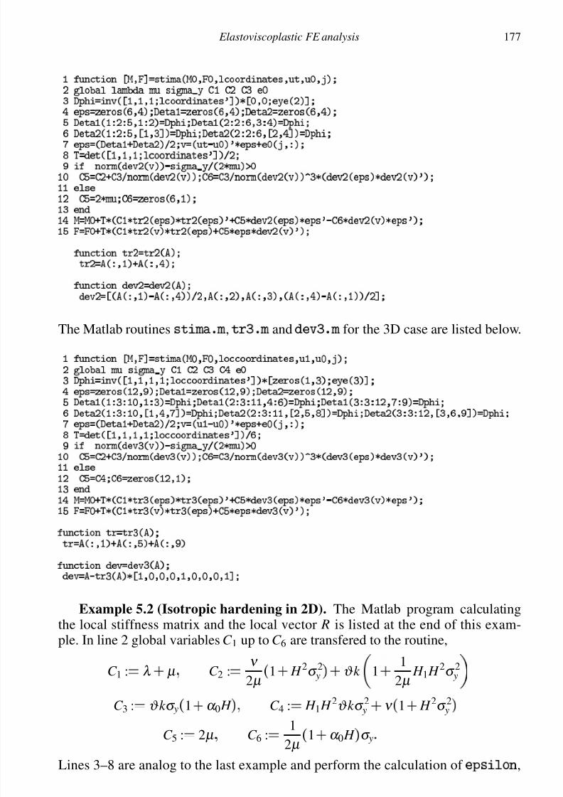
8/10/2019 2002-CC KR-Elastoviscoplastic FE Analysis in Matlab
http://slidepdf.com/reader/full/2002-cc-kr-elastoviscoplastic-fe-analysis-in-matlab 21/36
Elastoviscoplastic FE analysis 177
The Matlab routines
,
and
for the 3D case are listed below.
Example 5.2 (Isotropic hardening in 2D). The Matlab program calculatingthe local stiffness matrix and the local vector R is listed at the end of this exam-ple. In line 2 global variables C 1 up to C 6 are transfered to the routine,
C 1 : λ µ C 2 :
ν
2µ 1 H 2σ 2 y ϑ k
1
1
2µ H 1 H 2σ 2 y
C 3 :
ϑ k σ y
1
α 0 H
C 4 :
H 1 H 2ϑ k σ 2 y
ν
1
H 2σ 2 y
C 5 :
2µ C 6 :
1
2µ
1
α 0 H
σ y
Lines 3–8 are analog to the last example and perform the calculation of
,

8/10/2019 2002-CC KR-Elastoviscoplastic FE Analysis in Matlab
http://slidepdf.com/reader/full/2002-cc-kr-elastoviscoplastic-fe-analysis-in-matlab 22/36
178 C. Carstensen and R. Klose
define the vector v and determine the element area T . In line 9 the fall differentiationis performed. If
dev
v
C 6
0 the plastic phase occurs, otherwise the elasticphase. Depending on the result of this distinction, constants C 7 and a vector C 8 aredefined by
C 7 :
C 3
C 2 dev
v
C 4
C 2 if dev
v
C 6
0
C 5 else(5.14)
C 8 j :
C 3 C 2 dev
v
3 ε ϕ j
: v
if dev
v C 6
0
0 0 0 0 0 0
T else.(5.15)
In lines 14 and 15 an update of the local stiffness matrix and the first summand of the local vector R is performed. The components of the local stiffness matrix read
M jk
T
C 1 tr
ε ϕ j
tr ε ϕ k C 7 dev
ε ϕ j
: ε ϕ k
C 8 j dev
v
: ε ϕ k
(5.16)The components of the first summand of the vector R read
R j T
C 1 tr
v
tr
ε
ϕ j
C 7 dev
v
: ε
ϕ j
(5.17)
The Matlab routine
is listed below.
Example 5.3 (Kinematic hardening in 2D). The Matlab program calculatingthe local stiffness matrix and the local vector R is listed at the end of this example.In line 2 global variables C 1 up to C 4 are transfered to the routine,
C 1 : λ µ C 2 :
ϑ kk 1
2ν
ϑ k
ϑ kk 1
2µ
ν
µ
C 3 :
ϑ k σ yϑ k
ϑ kk 1
2µ
ν
µ C 4 :
2µ
Lines 3–8 are analog to the last example. The strain tensor
is calcu-lated, and matrices v and v1 are defined, with v :
ε ε ε
Uϑ U0
1σ σ σ 0, v1 :

8/10/2019 2002-CC KR-Elastoviscoplastic FE Analysis in Matlab
http://slidepdf.com/reader/full/2002-cc-kr-elastoviscoplastic-fe-analysis-in-matlab 23/36
Elastoviscoplastic FE analysis 179
1
2µ α α α 0. In line 9 the fall differentiation is performed. If dev
v σ y
2µ
0the plastic phase occurs, otherwise the elastic phase. Depending on the result of thisdistinction, a constant C 5, a vector C 6 and a Kronecker delta d are defined by
C 5 :
C 3
dev v
C 2 if dev v
σ y 2µ 0C 4 else
(5.18)
C 6 j :
C 3 dev
v
3
ε
ϕ j
: v
if dev
v σ y
2µ
0
0 0 0 0 0 0
T else
(5.19)
d :
1 if dev
v σ y
2µ
0
0 else.(5.20)
In lines 14 and 15 an update of the local stiffness matrix and the first summand of the local vector R is performed. The components of the local stiffness matrix read
M jk T
C 1 tr
ε
ϕ j
tr
ε
ϕ k
C 5 dev
ε
ϕ j
: ε
ϕ k
C 6 j dev
v
: ε
ϕ k
(5.21)The components of the first summand of the vector R read
R j T
C 1 tr
v
tr
ε
ϕ j
C 5 dev
v
: ε
ϕ j
d dev
α 0
: ε
ϕ j
(5.22)
The Matlab routine
is listed below.
6. POSTPROCESSING
6.1. Displaying the solution
Our two dimensional problems model the plain stress condition. In that case, thecomplete stress tensor σ
3 3sym has the form
σ
σ 11 σ 12 0σ 12 σ 22 0
0 0 0
8/10/2019 2002-CC KR-Elastoviscoplastic FE Analysis in Matlab
http://slidepdf.com/reader/full/2002-cc-kr-elastoviscoplastic-fe-analysis-in-matlab 24/36
180 C. Carstensen and R. Klose
with σ 33
12λ µ λ σ 11 σ 22
. It then follows for devσ 2, where dev A :
A
13
tr AId 3 3 and A
:
∑n j
k
1 A2 jk
1 2is the Frobenius norm, that
devσ 2
µ 2
6 µ λ 2
12
σ 11 σ 22
2
2 σ 212 σ 11σ 22
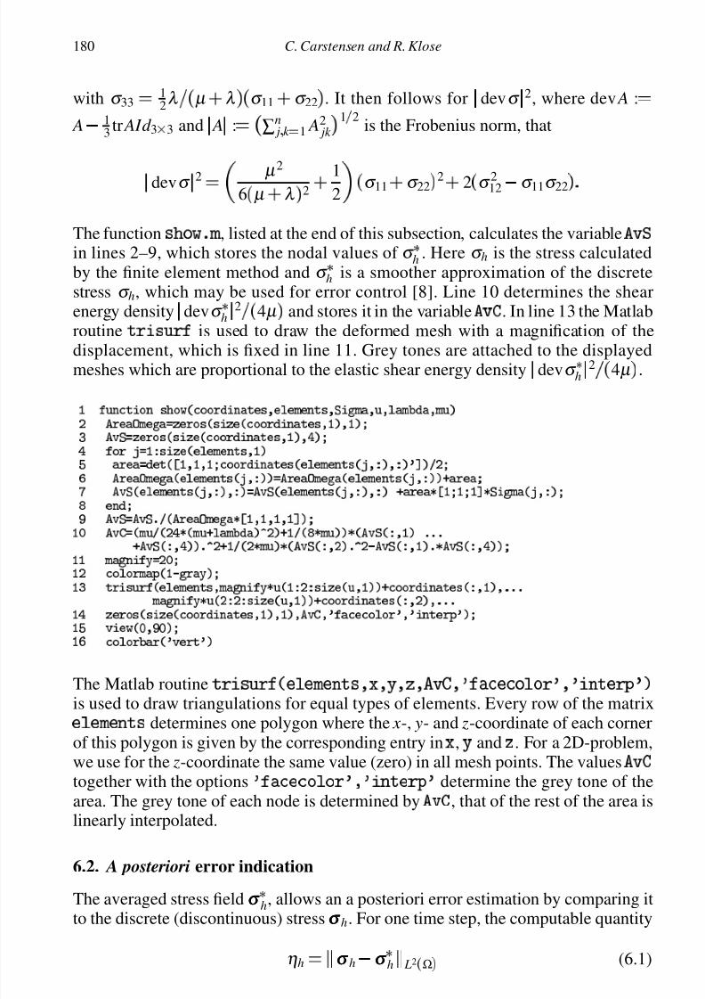
The function
, listed at the end of this subsection, calculates the variable
in lines 2–9, which stores the nodal values of σ h . Here σ h is the stress calculatedby the finite element method and σ h is a smoother approximation of the discretestress σ h, which may be used for error control [8]. Line 10 determines the shearenergy density
devσ h
2
4µ
and stores it in the variable
. In line 13 the Matlabroutine
is used to draw the deformed mesh with a magnification of the
displacement, which is fixed in line 11. Grey tones are attached to the displayedmeshes which are proportional to the elastic shear energy density
devσ h
2
4µ .
The Matlab routine
is used to draw triangulations for equal types of elements. Every row of the matrix
determines one polygon where the x-, y- and z-coordinate of each cornerof this polygon is given by the corresponding entry in
,
and
. For a 2D-problem,we use for the z-coordinate the same value (zero) in all mesh points. The values
together with the options
determine the grey tone of thearea. The grey tone of each node is determined by
, that of the rest of the area islinearly interpolated.
6.2. A posteriori error indication
The averaged stress field σ σ σ h, allows an a posteriori error estimation by comparing itto the discrete (discontinuous) stress σ σ σ h. For one time step, the computable quantity
ηh σ σ σ h
σ σ σ h L2 Ω
(6.1)
8/10/2019 2002-CC KR-Elastoviscoplastic FE Analysis in Matlab
http://slidepdf.com/reader/full/2002-cc-kr-elastoviscoplastic-fe-analysis-in-matlab 25/36
Elastoviscoplastic FE analysis 181
defines the error estimate [8] (for pure Dirichlet conditions – Neumann boundaryconditions require modifications [9])
σ σ σ
σ σ σ h L2
Ω
C ηh
(6.2)
Here,σ σ σ h may be any piecewise affine and globally continuous stress approximation.It is emphasized that the error bound (6.2) holds only if the time-discretization erroris neglected. It is generally believed that the accumulation error (in time) cannot becaptured by averaging (in space). However the quantity ηh may monitor the localspatial approximation error and a large size of ηh indicates a larger spatial error andmotivates refinements.
Theorem 6.1 (Efficeny). Assume that the stress field σ σ σ at time t is smooth, i.e.
σ σ σ H 1 Ω; d
d sym , then ηh is an efficient error estimator up to higher order terms inthe sense that
ηh
4 σ σ σ σ σ σ h L2
Ω
h o t
(6.3)
where generically h o t O h2Dσ L2
Ω
σ σ σ
σ σ σ h L2
Ω
.
Proof. The triangle inequality provides, for all τ τ τ h which are globally continousand
-piecewise affine (like σ σ σ h), that
σ σ σ h
τ τ τ h
L2 Ω
σ σ σ
σ σ σ h
L2 Ω
σ σ σ
τ τ τ h
L2 Ω
σ σ σ
σ σ σ h
L2 Ω
h
o
t
(6.4)
for the nodal interpolation τ τ τ h I σ σ σ of σ σ σ [5]. One can prove that (with τ τ τ h globalycontinous and
-piecewise affine but arbitrary otherwise)
η M :
minτ τ τ h
σ σ σ h
τ τ τ h L2
Ω
σ σ σ h
σ σ σ h L2
Ω
4η M
This is shown for ab arbitrary constant in [6,14,16] and for the constant 4 and quitegeneral boundary conditions in [7]. The main argument is a (local) inverse estimate,
caused by equivalence of norms on finite dimensional vector spaces.The combination of the two inequalities leads to
ηh σ σ σ
σ σ σ h L2
Ω
4η M
4 σ σ σ
σ σ σ h L2
Ω
4 σ σ σ
τ τ τ h L2
Ω
for any τ τ τ h, in particular for τ τ τ h I σ σ σ .
It is emphasized once more that the reliability (6.2) is problematic and holdsonly for one time step and for large hardening and large viscosity [8].
The Matlab routine at the end of this subsection calculates at time t t 1.Lines 3–4 initialise
ω z
, the patch of the hat function at node z, which is stored in and σ σ σ h, which is stored in . Line 5 determines weights and barycen-tric coordinates by a two dimensional quadrature rule. In our algorithm we haveσ σ σ h
z
ω zσ σ σ h d x
ω z
. Lines 6–10 calculate the area of the elements (line 7), the

8/10/2019 2002-CC KR-Elastoviscoplastic FE Analysis in Matlab
http://slidepdf.com/reader/full/2002-cc-kr-elastoviscoplastic-fe-analysis-in-matlab 26/36
182 C. Carstensen and R. Klose
patch size ω z
(line 8) and
ω zσ σ σ h d x (line 9) by a loop over all elements. In line 11,
σ σ σ h is obtained by dividing
ω zσ σ σ h d x through the patch size. Lines 12–16 compute
, where for σ σ σ h four interpolation points are used on each element T .
7. NUMERICAL EXAMPLES
7.1. On a plate with circular hole
A two dimensional squared plate with a hole, Ω 2 2
2 B 0 1 is submitted
to time dependent surface forces g
t
600t
n at the top ( y
2) and the bottom( y
2), where n denotes the outer normal to ∂ Ω. The rest of the boundary is
traction free. As the problem is symmetric only a quarter of Ω is discretised. The
boundary conditions are specified in files
,
, and
:

8/10/2019 2002-CC KR-Elastoviscoplastic FE Analysis in Matlab
http://slidepdf.com/reader/full/2002-cc-kr-elastoviscoplastic-fe-analysis-in-matlab 27/36
Elastoviscoplastic FE analysis 183
0.1
0.2
0.3
0.4
0.5
0.6
−0.5 0 0.5 1 1.5 2 2.5−0.5
0
0.5
1
1.5
2
2.5
Γ
Γ
Γ N
Γ D
N
N
Γ D
Figure 3. Deformed mesh for membrane with hole in the example of Subsection 7.1 calculated with3474 degrees of freedom. The grey tone visualises devσ h
2 4µ as described in Subsection 6.1.
This numerical example from [17] models perfect viscoplasticity with Young’smodulus E
206900, Poisson’s ratio ν
0
29, yield stress σ y
450 and vanishinginitial data for the stress tensor σ 0.
The solution is calculated with 3474 degrees of freedom in the time intervalfrom t
0 to t
0
4 by the implicit Euler method in 8 uniform steps of lengthk 1 20. The material remains elastic between t 0 and t 0 2. Figure 3 showsthe deformed mesh at t
0
2, Table 1 shows the number of iterations in Newton’s
method and the estimated error for each time step.Table 1.
Number of iterations and indicated error for membrane with
hole in the example of Subsection 7.1 for various time steps.
step iterations η
σ h
σ h 2
σ h 2
1 1 0.04322 1 0.04323 1 0.04324 5 0.0436
5 5 0.04626 5 0.05057 6 0.05658 6 0.0642
8/10/2019 2002-CC KR-Elastoviscoplastic FE Analysis in Matlab
http://slidepdf.com/reader/full/2002-cc-kr-elastoviscoplastic-fe-analysis-in-matlab 28/36
184 C. Carstensen and R. Klose
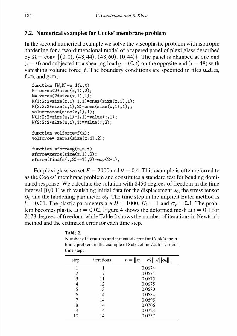
7.2. Numerical examples for Cooks’ membrane problem
In the second numerical example we solve the viscoplastic problem with isotropichardening for a two-dimensional model of a tapered panel of plexi glass described
by Ω
conv
0
0
,
48
44
,
48
60
,
0
44
. The panel is clamped at one end( x
0) and subjected to a shearing load g
0 t
on the opposite end ( x
48) withvanishing volume force f . The boundary conditions are specified in files
,
, and
:
For plexi glass we set E
2900 and ν
0
4. This example is often referred to
as the Cooks’ membrane problem and constitutes a standard test for bending domi-nated response. We calculate the solution with 8450 degrees of freedom in the timeinterval [0,0.1] with vanishing initial data for the displacement u0, the stress tensorσ 0 and the hardening parameter α 0. The time step in the implicit Euler method isk
0
01. The plastic parameters are H
1000, H 1
1 and σ y
0
1. The prob-lem becomes plastic at t
0
02. Figure 4 shows the deformed mesh at t
0
1 for2178 degrees of freedom, while Table 2 shows the number of iterations in Newton’smethod and the estimated error for each time step.
Table 2.
Number of iterations and indicated error for Cook’s mem-
brane problem in the example of Subsection 7.2 for various
time steps.
step iterations η
σ h
σ h 2
σ h 2
1 1 0.06742 7 0.06743 11 0.06754 12 0.06755 13 0.0680
6 14 0.06847 14 0.06958 14 0.07069 14 0.0723
10 14 0.0737

8/10/2019 2002-CC KR-Elastoviscoplastic FE Analysis in Matlab
http://slidepdf.com/reader/full/2002-cc-kr-elastoviscoplastic-fe-analysis-in-matlab 29/36
Elastoviscoplastic FE analysis 185
0.5
1
1.5
2
2.5
3
x 10−5
−10 0 10 20 30 40 50−10
0
10
20
30
40
50
60
70
Γ
Γ
Γ Γ N N
N
D
Figure 4. Deformed mesh for Cooks’ membrane problem in the example of Subsection 7.2 calculated
with 2178 degrees of freedom. The grey tone visualises
devσ
h
2
4µ
as described in Subsection 6.1.
7.3. Numerical example for axissymmetric ring
The third numerical example is taken from [4]. We solve a viscoplastic model withkinematic hardening. The geometry is a two-dimensional section of a long tubewith inner radius 1 and outer radius 2 (Fig. 6). We have no volume force, f
0 buttime depending surface forces g1
r
ϕ
t
ter and g2
r
ϕ
t
t
4er . The systemis required to keep centered at the origin and rotation is prohibited. The boundaryconditions are specified in files
,
, and
:
8/10/2019 2002-CC KR-Elastoviscoplastic FE Analysis in Matlab
http://slidepdf.com/reader/full/2002-cc-kr-elastoviscoplastic-fe-analysis-in-matlab 30/36
186 C. Carstensen and R. Klose
The exact solution is
u r ϕ t ur r t er
σ r ϕ t σ r r t er er σ ϕ eϕ eϕ
p r ϕ t Pr r t er er eϕ eϕ
(7.1)
with er
cosϕ
sinϕ
, eϕ sinϕ
cosϕ
and with a
µ
λ ,
2µ
2µ
λ ,
ur
r
t
t
2µ r
1
3
I
R
t
r
4a
µ r
r
R
t
t
2µ r
1
3 I R t
4r
4a
µ r
I r r r R t
(7.2)
σ r r t
t
r 2
8
3a I R t
1
4
1
r 2
r R t
t
r 2
8
3 a
I
R
t
1
1
r 2
2a
I
r
r
R
t
(7.3)
σ ϕ r t
∂ r σ r
∂ r (7.4)
Pr r t
0 r R t
σ y
2
a
k 1
1 R2
r 2
r
R
t
(7.5)
I r
σ y
2
a
k 1
ln r
1
2 R2
r 2 R2
(7.6)
With α
4a
3 a k 1
, the radius of the plastic boundary R t
is the positiveroot of
f R 2α ln R α
1 R2
α
2
σ yt
(7.7)

8/10/2019 2002-CC KR-Elastoviscoplastic FE Analysis in Matlab
http://slidepdf.com/reader/full/2002-cc-kr-elastoviscoplastic-fe-analysis-in-matlab 31/36
Elastoviscoplastic FE analysis 187
Table 3.
Number of iterations, indicated error, and exact error for axissymmetric ring in
the example of Subsection 7.3. This numerical example validates our claim that
η can be an accurate error guess.
step iterations e
σ
σ h 2
σ 2 η
σ h
σ
h 2
σ h 2 e
η1 1 0.0512 0.0510 1.00
. . . . . . . . . . . . . . .
14 1 0.0512 0.0510 1.0015 3 0.0521 0.0515 1.0116 4 0.0533 0.0529 1.0117 4 0.0549 0.0543 1.0118 4 0.0565 0.0560 1.0119 4 0.0584 0.0579 1.01
The material parameters are E
70000 for Young’s modulus, ν
0
33 for Pois-son’s ratio and the yield stress is σ y
0
2.The solution is calculated in the time interval [0,0.2] with 3202 degrees of free-
dom and vanishing initial data for the displacement u0, the stress tensor σ 0 and thehardening parameter α 0. The time step in the implicit Euler method is k
0
01. Thehardening parameter is k 1
1. The material becomes plastic at t
0
16. Table 3shows the error and the estimated error for the different time steps together withthe number of iterations in Newton’s method. Figure 5 shows the deformed mesh at
t
0
18, displacements magnified by the factor 10.
7.4. Numerical example in three dimensions
As a three-dimensional example we solve a perfect viscoplastic problem on the cube
0
1
3
0
0
5
3. The face with x
1 is Dirichlet boundary, the rest is Neumannboundary. The volume force f is zero while the surface force is g tn, if the normalvector n points in y-direction. The boundary conditions are specified in files
,
, and
:

8/10/2019 2002-CC KR-Elastoviscoplastic FE Analysis in Matlab
http://slidepdf.com/reader/full/2002-cc-kr-elastoviscoplastic-fe-analysis-in-matlab 32/36
188 C. Carstensen and R. Klose
0.5
1
1.5
2
2.5
3
3.5
4
4.5
5
5.5
x 10−7
−0.5 0 0.5 1 1.5 2 2.5−0.5
0
0.5
1
1.5
2
2.5
Figure 5. Deformed mesh for axissymmetric ring in the example of Subsection 7.3 calculated with3202 degrees of freedom. The grey tone visualises devσ h
2 4µ as described in Subsection 6.1.
2gf=0
Ω
g1
1 2
E
70000ν
0
33
σ y
0
2
k 1
1
g1 ter
g2 t
4er
Figure 6. Axissymmetric ring in the example of Subsection 7.3 with initial triangulation of a quarterof the ring endowed with symmetrie boundary conditions.
8/10/2019 2002-CC KR-Elastoviscoplastic FE Analysis in Matlab
http://slidepdf.com/reader/full/2002-cc-kr-elastoviscoplastic-fe-analysis-in-matlab 33/36
Elastoviscoplastic FE analysis 189
−0.5
0
0.5
1
−0.20
0.20.4
0.60.8
11.2
−0.2
0
0.2
0.4
0.6
0.8
1
1.2
xy
z
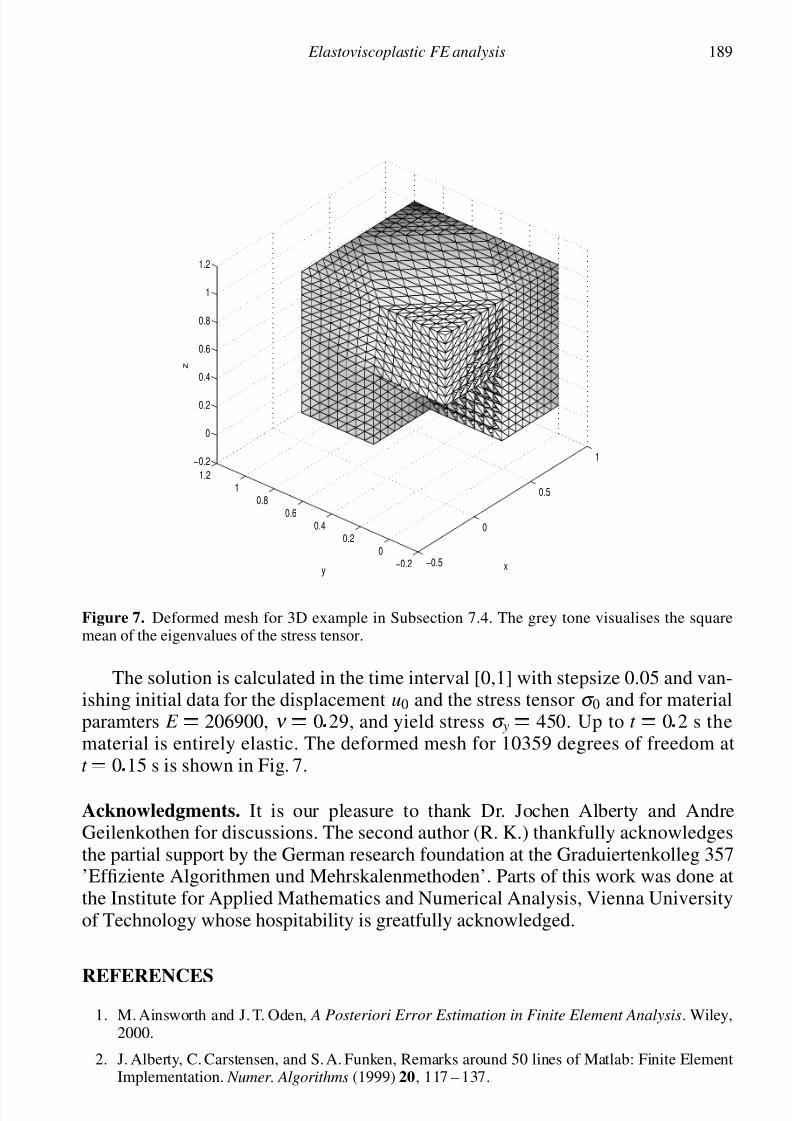
Figure 7. Deformed mesh for 3D example in Subsection 7.4. The grey tone visualises the squaremean of the eigenvalues of the stress tensor.
The solution is calculated in the time interval [0,1] with stepsize 0.05 and van-ishing initial data for the displacement u0 and the stress tensor σ 0 and for materialparamters E
206900, ν
0
29, and yield stress σ y
450. Up to t
0
2 s thematerial is entirely elastic. The deformed mesh for 10359 degrees of freedom att
0
15 s is shown in Fig. 7.
Acknowledgments. It is our pleasure to thank Dr. Jochen Alberty and AndreGeilenkothen for discussions. The second author (R. K.) thankfully acknowledgesthe partial support by the German research foundation at the Graduiertenkolleg 357’Effiziente Algorithmen und Mehrskalenmethoden’. Parts of this work was done atthe Institute for Applied Mathematics and Numerical Analysis, Vienna Universityof Technology whose hospitability is greatfully acknowledged.
REFERENCES
1. M. Ainsworth and J. T. Oden, A Posteriori Error Estimation in Finite Element Analysis. Wiley,2000.
2. J. Alberty, C. Carstensen, and S. A. Funken, Remarks around 50 lines of Matlab: Finite ElementImplementation. Numer. Algorithms (1999) 20, 117 – 137.

8/10/2019 2002-CC KR-Elastoviscoplastic FE Analysis in Matlab
http://slidepdf.com/reader/full/2002-cc-kr-elastoviscoplastic-fe-analysis-in-matlab 34/36
190 C. Carstensen and R. Klose
3. J. Alberty, C. Carstensen, S. A. Funken, and R. Klose, Matlab Implementation of the Finite Ele-ment Method in Elasticity. Berichtsreihe des Mathematischen Seminars, Kiel, 2000, 00–21.
4. J. Alberty, C. Carstensen, and D. Zarrabi, Adaptive numerical analysis in primal elastoplasticitywith hardening. Comp. Methods Appl. Mech. Engrg. (1999) 171, 175 – 204.
5. S. C. Brenner and L. R. Scott, The mathematical theory of finite element methods. Texts in Ap- plied Mathematics, Vol. 15. Springer, New York, 1994.
6. C. Carstensen, On the History and Future of Averaging Techniques in A Posteriori FE ErrorAnalysis. In: ZAMM Proceedings of Annual GAMM Conference, 2002 (to appear).
7. C. Carstensen, First-order averaging techniques for a posteriori Finite Element error control onunstructured grids are efficient and reliable, 2002 (submitted).
8. C. Carstensen and J. Alberty, Averaging techniques for reliable a posteriori FE-error control inelastoplasticity with hardening? Berichtsreihe des Mathematischen Seminars, Kiel, 2000, 00–23.
9. C. Carstensen and S. A. Funken, Averaging technique for FE-a posteriori error control in elas-
ticity. Part I: Conforming FEM. Comp. Meth. Appl. Mech. Engrg. (2001) 190, 2483 – 2498. PartII: λ -independent estimates. Comp. Meth. Appl. Mech. Engrg. (2001) 190, 4663 – 4675. Part III:Locking-free conforming FEM. Comp. Meth. Appl. Mech. Engrg. (2001) 191, 861 – 877.
10. P. G. Ciarlet, The Finite Element Method for Elliptic Problems. North-Holland, 1978.
11. W. Han and B. D. Reddy, Plasticity: Mathematical Theory and Numerical Analysis. Springer,New York, 1999.
12. L. Langemyr et. al., Partial Differential Equation Toolbox User’s Guide. The Math. Works, 1995.
13. D. Redfern and C. Campbell, The Matlab5 Handbook . Springer, 1998.
14. R. Rodriguez, Some remarks on Zienkiewicz-Zhu estimator. Int. J. Numer. Meth. in PDE , 10,625 – 635.
15. J. C. Simo and T. J. R. Hughes, Computational Inelasticity. Springer, 2000.
16. R. Verfurth, A Review of A Posteriori Error Estimation and Adaptive Mesh-Refinement Tech-niques. Wily-Teubner, 1996.
17. P. Wriggers et al., Benchmark Perforated Tension Strip. In: Communication in Talk at ENU- MATH Conference in Heidelberg, 1997.
8. APPENDIX
8.1. Main program in Example 1

8/10/2019 2002-CC KR-Elastoviscoplastic FE Analysis in Matlab
http://slidepdf.com/reader/full/2002-cc-kr-elastoviscoplastic-fe-analysis-in-matlab 35/36
Elastoviscoplastic FE analysis 191
8.2. Calculation of the stress in Example 1
8.3. Main program in Example 4
8.4. Calculation of the stress in Example 4
8/10/2019 2002-CC KR-Elastoviscoplastic FE Analysis in Matlab
http://slidepdf.com/reader/full/2002-cc-kr-elastoviscoplastic-fe-analysis-in-matlab 36/36
192 C. Carstensen and R. Klose