20 questions and solutions—operational research (or) · pdf filequestions and...

20

Questions and solutions— operationalresearch (OR)

Summary

The Operational Research Society explains OR as development of a scientific model of a systemincorporating measurements of factors such as chance and risk, with which to predict and compare the outcomes of alternative strategies or means of control. In the main, the method issuited to those logistical problems that are highly dependent on detailed and accurate records ofperformance data and which can broadly be analysed and solved by mathematical programs.Combined with readily available computer software OR can positively assist in better construc-tion planning, resources allocation, economic analysis and performance evaluation to achievemarginal improvements in scheduling and control.

The following methods provide examples that demonstrate potential applications to con-struction management:

• Linear, integer, binary integer linear programming

• Simplex method, transportation and assignment

• Quadratic assignment programming

• Goal programming

• Non-linear programming

• Dynamic programming

• Decision trees and utility

• Markov processes

• Queuing theory, simulation

• Stock control, inventory under uncertainty

• Theory of games

561

MCM20 6/30/06 5:40 PM Page 561

Questions

Question 1 Linear programming illustrating maximisation

A building contractor produces two types of house for speculative building—detached andsemi-detached houses.The customer is offered several choices of architectural design and layoutfor each type. The proportion of each type of design sold in the past is shown in Table Q1.1. Theprofit on a detached house and a semi-detached house is £1000 and £800, respectively.

Table Q1.1 Proportion of sales.

Choice of design Detached Semi-detached

Type A 0.1 0.33Type B 0.4 0.67Type C 0.5

The builder has the capacity to build 400 houses per year. However, an estate of housing willnot be allowed to contain more than 75% of the total housing as detached.Furthermore,becauseof the limited supply of bricks available for Type B designs, a 200-house limit with this design isimposed.

(1) Determine how many detached and semi-detached houses should be constructed in ordertomaximise profits and state the optimum profit.

(2) Calculate the extra profit generated by increasing the capacity above 400 houses per year. Isthis a sensible policy if the cost of providing the additional resources is £1000 per house?

Question 2 Linear programming illustrating minimising

A workshop in servicing engines replaces two parts A and B in the proportions shown below at acost of £10 and £8 each, respectively. At least 10 per day of type A need to be completed and theworkshop has the capacity to handle 40 parts in total per day.

Part A requires 0.5 hours while B requires 0.2 hours and 10 hours is worked each day.

563

MCM20 6/30/06 5:40 PM Page 563

Part type Proportion

A 1/3B 2/3

(1) Determine how many parts of each type per day should be fitted in order to minimise pro-duction cost and state the optimum production cost.

(2) Is this a sensible policy if the workshop overtime costs are £30 per hour?

Question 3 Simplex method — constraints: ‘equal to or less than’

A construction crew of five workers is provided on site with two concrete delivery systems type Aand type B, and is paid respectively £50 and £60 per 100 m3 of concrete placed. The equipmentand labour resources production output rates are as follows:

Dumpers Crane Crew

Type A 12.5 m 3/hr 25 m3/hr 2 m3/hrType B 25 m 3/hr 20 m3/hr 0.13 m 3/hr

How should the delivery systems be organised to maximise income over the 40-hour workingweek?

Question 4 Simplex method — constraints: ‘greater than or equal to’

Solve the following problem of the type:

2x + 3y≥ 14

8x + 5y≥ 40

x ≥ 0

y≥ 0

Maximise 1.5x + y.

Question 5 Simplex method — constraints: ‘greater than or equal to’

Find the solution to Question 4 as a minimum.

564 Self-learning exercises

MCM20 6/30/06 5:40 PM Page 564

Question 6 Integer linear programming

Solve Question 3 as an integer problem

Question 7 Binary integer linear programming

A further application of binary variables in the formof 0 and 1 values can also be very useful formodelling logical conditions. Solve Questions 3–6 with the following additional information:

• System A set up costs £50 with a maximum delivery capacity 175 m3/week.

• System B set up costs £125 with a maximum delivery capacity 700 m3/week.

Question 8 Transportation problem

A civil engineering contractor is engaged to carry out the earth moving work for the construc-tion of a new section of motorway. Fill material can be supplied from three borrow pits l, 2 and 3located near the works, up to a maximum of 60 000, 80 000 and 120 000 m3 from each, respec-tively. The material is to be delivered to three locations, A, B and C along the road, and each re-quires 90 000, 50 000 and 40 000 m3, respectively. The costs in pence per cubic metre for deliveryof the material from the pits to each of the three sites are shown in Table Q8.1.

Determine the best arrangements, for supply and delivery of the material, if the objective is tominimise cost.

Question 9 Assignment problem

A contractor has been successful in obtaining five new projects. The projects, however, are dif-ferent in value, type of work and complexity.As a result, the experience and qualities required ofthe project manager for each will be different. After careful considerations, five managers are selected and their skills assessed against each project. Each manager is scored on a points scale,with a maximum of 100 marks indicating that the manager is highly suitable, and zero mark unsuitable for the work. The individual assessments are shown in Table Q9.1.

Which managers should be allocated to which projects, if the company wishes to distributethem in the most effective way?

Questions 565

Table Q8.1 Supply and delivery of fill material.

Quantity required at sites Quantity supplied from pits

A (90 000 m 3) B (50 000 m 3) C (40 000 m 3)

1 70p 40p 100p 60 000 m 3

2 50p 30p 90p 80 000 m 3

3 60p 50p 90p 120 000 m 3

MCM20 6/30/06 5:40 PM Page 565

Question 10 Assignment when number of agents and tasks differ

Solve Question 9 if only four managers 1, 2, 3 and 4 are available.

Question 11 Goal programming

If in Question 1 the first priority is to build 200 houses of Type B design, and second priority tocomplete no more than 400 in total, determine the optimum mix of housing.

Question 12 Non-linear programming

Problems not having linear properties are called non-linear and comprise relationships withvariables expressed to powers other than one, e.g. quadratic form (squared), multiplied or divided by each other or cubed, etc. This occurs when either the objective function or the constraints or both are non-linear. Finding optimal solutions requires sophisticated methods ofcalculation and may provide only local optimum results.

(a) Maximise x2− 2x + y2− 6y(b) Minimise x2− 2x + y2− 6y

subject to the constraints

2x + y< 8

x ≥ 0, y≥ 0

Question 13 Quadratic assignment problem

In order to avoid the quadratic terms in a non-linear problem, expressions can sometimes be re-arranged into the assignment-type linear form to provide the solution. For example:


Table Q9.1 Individual assessments.

Manager

(1) (2) (3) (4) (5)

Project (A) 75 28 61 48 59(B) 78 71 51 35 19(C) 73 61 40 49 68(D) 55 50 52 48 63(E) 71 60 61 74 70

MCM20 6/30/06 5:40 PM 66

Profitability Indifference value (p) Utility value

18% 1 1016% 0.95 9.512% 0.6 6.010% 0.4 4.05% 0.30 3.00% 0 0

Determine which outcome the company might prefer.

Question 18 Markov processes

A plant firm’s workshop has been recording the running performance of a machine at one hourperiods and determined that the probability state of the machine being in a running or downstate relates to its state in the previous period as follows:

To running To down

From running 0.85 0.15From down 0.2 0.8

During maintenance the cause of breakdown was revealed to be failure of a specific part,which if replaced is assessed to improve the transition probabilities as shown below:

To running To down

From running 0.9 0.1From down 0.3 0.7

(1) Determine the steady-state probabilities of the running and downtime states.(2) What are the steady-state probabilities after the failed part is replaced?(3) If the cost of downtime for a one-hour period is £100, determine the break even price that

can be paid for the new component (including its fitting) on a time-period basis.

Question 19 Queuing

Trucks arrive at an excavator, where observations over a 136-minute period show that the num-bers of trucks arriving per minute (i.e. time period) are 0, 1, 2, 3, 4 or more and have correspon-ding frequencies 78,41,15,2,0.Thirty service (loading) times are also recorded as follows: 0.5,1,1.5, 2, 2.5, 3 minutes or less, and the corresponding frequencies are 9, 9, 7, 3, 1, 1.

Determine whether the observed data for arrival times and service time represent respec-tively Poisson and Exponential probability distributions.

Calculate the average time trucks spent in the system (i.e. waiting and loading).Calculate the average number of trucks in the system:

Questions 569

MCM20 6/30/06 5:40 PM Page 569

(a) if the calling ie. arrivals population is infinitely large(b) if there are only four trucks in the fleet

Determine the optimum number of excavators to minimise cost, when the hire costs of an excavator and truck are respectively £50 and £60 per hour and a maximum of 3 excavators areavailable.

Question 20 Simulation

Tr ucks arrive at a batching plant from distribution points in an area serviced by a ready-mixedconcrete depot. The arrival time intervals of the trucks are observed and yield the followingresults:

Arrival time interval (min) Frequency (%)

2 103 154 305 256 20

The times taken to load the trucks, which are either 3 or 6 m3 capacity, are fairly constant at 3and 5 min respectively, and both types are equally represented at the depot.

If the batching plant loads each truck immediately it arrives, in the order that it arrives, calcu-late the total time likely that the mixer and trucks will be waiting in any one period of two hoursselected at random.

Question 21 Stock control — simple case

Stocks of cement on a construction site are allowed to run down to a level of 3 tonnes beforebeing replenished. Cement is used steadily at 50 tonnes per week. Cement costs £15 per tonneand the cost of storage and deterioration per week is 10% of the cement price. Each time cementis ordered there is a cost of processing this order of £1.

(1) How much cement should be ordered each time?(2) What is the cost of ordering and storing the cement?

Question 22 Stock control — continuous usage

A manufacturer of pre cast concrete units is required to supply 1000 pre cast floor beams eachweek to a large building contract.The building contractor has very little storage space on site andthus requires the beams to be delivered at the rate at which they can be placed in position. Themanufacturer has the capacity to produce 2500 beams per week. The cost of storing a singlebeam per week is 1p and the cost of setting up the equipment for a production run is £50.


MCM20 6/30/06 5:40 PM Page 570

(1) What is the optimum number of units to produce in a production run?(2) What is the total cost of producing and storing the contractor’s requirements for beams?(3) How frequently should production runs be made?

Question 23 Stock control — shortages

A building project calls for the steady supply of 50 000 bricks each week; the price of the bricks is£30 per thousand.The brick supplier usually keeps sufficient stocks in the yard to meet customerdemand and the cost of holding 1000 bricks per week is 10% of their cost price. The cost to thesupplier each time a new order is processed is £10. However, sometimes the delivery date cannotbe met so to make up the backlog there are special deliveries to the customer as soon as the sup-plier is able to continue with the order. The extra cost incurred by the supplier in this situation is£10 per 1000 bricks.

(1) Calculate the economic order quantity for the supplier.(2) Calculate the total cost per week to the supplier of stockholding and processing orders.(3) Calculate the level to which stock on site is topped up.

Question 24 Stock control — discounts

(T his question should not be attempted before trying Question 21.)Aggregate is used on a construction site at the rate of 2000 tonnes per month. The cost of

ordering is £20 and the cost of storing the material on site is 50% of its purchase cost. The cost per tonne depends on the total quantity ordered as follows:

(a) (b) (c)

Less than 500 tonnes 500–999 tonnes 1000 or more£1.21 per tonne £1.00 per tonne £0.81 per tonne

Calculate the optimum order quantity and the optimum total cost per month of purchasing,storing and ordering the material.

Question 25 Inventory under uncertainty

Demand for equipment maintenance can vary between 95 and 105 items per week, accordinglythe workshop manager budgets midway for servicing 100 items per week (Q) at a cost of£200 each.

Each item serviced is charged to customers at £300. If demand exceeds the plan, during theweek customers are turned away. Conversely, when demand is less than plan the workshop re-sources are under-utilised but the budgeted costs are still incurred.

Suppose the probabilities of demand are those shown below. Determine the Optimal OrderQuantity Q.

Questions 571

MCM20 6/30/06 5:40 PM Page 571

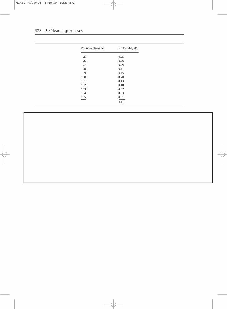
Possible demand Probability (Pr)

95 0.0596 0.0697 0.0998 0.1199 0.15

100 0.20101 0.13102 0.10103 0.07104 0.03105 0.01

1.00

Question 26 Theory of games

Mixed strategy

A listed company A has two operating divisions,plant and construction,which have come undertakeover speculation from company B. Company A has sufficient resources to successfully resista bid for one or the other division. Similarly, the predator firm B is capable of mounting a suc-cessful takeover of either plant or construction. The construction division is worth £3 m, theplant division £2 m,and nothing is lost if the divisions ultimately remain under the ownership ofthe parent A firm.

Determine the value of the game and the best strategies for A and B.


MCM20 6/30/06 5:40 PM Page 572

Solutions

Lindo software at www.Lindo.com, and similar proprietary products, which facilitate interac-tive use from the keyboard or customised subroutines linked directly to form an integrated pro-gram, have been adopted where appropriate in this text.

Solution 1 Linear programming illustrating maximisation

This type of problem can be readily solved using the linear programming mathematical tech-nique developed to determine a maximum value such as profit or minimum cost, where avail-ability of the associated resources is constrained.

The descriptor ‘linear’ implies proportionality while ‘programming’ refers to the mathemat-ical process of determining an optimum allocation of resources.

Problem formulation

The steps needed to be undertaken in solving a linear programming problem are as follows;

(1) Define the decision variables, these being the controllable inputs in both the objective and constraint equations and which describe the number or amounts of each item to produce.

(2) Describe the objective function in terms of the decision variables, this being the subject tobe optimised, e.g. profit, output, etc. expressed as a formula.

(3) Establish the constraint value for each resource that has an imposed limit and express interms of the decision variables.

(4) Solve for the decision variables and substitute into the objective function and determine itsquantity or amount.

In this first problem the decision variables can be established as follows:

Part (a)

Decision variables:

Let X = number of detached houses constructedY = number of semi-detached houses constructed

573

MCM20 6/30/06 5:40 PM Page 573

Row 1. Total profit objective function:

MAX = 1000 × X + 800 × Y

Rows 2 and 3. Constraints to prevent negative values of X and Y:

X > 0Y > 0

Row 4. Constraint on the builder’s capacity:

X + Y ≤ 400

Row 5. Constraint on detached:

X ≤ 0.75 × (X + Y)

Row 6. Constraint on B type design:

0.4 × X + 0.67 × Y < = 200

The equations plotted graphically in Fig.S1.1 illustrate the area of feasible solutions and theoptimum profit is the solution which maximises the objective function 1000X+ 800Y.

Clearly various combinations of X and Y will lead to the same profit. For example, a profit of£160 000 is obtained for all pairs of X and Y lying on the line 1000X + 800Y = 160 000.


X

Y

Maximising

400

400

TP = 300, 100

Feasibleregion

Objective function

Max = 1000X + 800Y

X + Y ≤ 400

2/5(X ) + 2/3(Y

) ≤ 200

¼X – ¾Y ≤ 0

Fig. S1.1

MCM20 6/30/06 5:40 PM Page 574

The profit will continue to grow with any line drawn parallel to the objective function, mov-ing away from the origin until the line is just tangential to the feasible area, the objective functionthen being at the tangential point.

The co-ordinates of X and Y at the tangent point (TP) are 300 and 100 respectively, whichwhen substituted into the objective function yield a profit of £380 000. In other words, to opti-mise profit, 300 detached and 100 semi-detached is the best mix. The amount of each design isshown below.

Summary

Objective value: £380 000Variable ValueX 300Y 100Row Slack or surplus1 380 0002 3003 1004 05 06 13

The above summary illustrates that the constraints for all rows were not violated in not beingnegative values.However, for row 6 the constraint equation of 0.4X + 0.67Y substituted with X,Yvalues of 300 and 100 respectively gives 200 − 0.4 × 300 + 0.67 × 1000 = 13, i.e. produces a slackamount of 13 houses, meaning that this resource is under-utilised.A negative, i.e. surplus, valuewould have indicated insufficient availability of this resource.

Part (b) Shadow prices or duality

Clearly there would be little point in increasing the limit of 200 houses on design type B, as theconstraints on rows 4 and 5 are presently fully utilised, i.e. no slack. However, it would be of in-terest to determine the effect on profit of increasing the limit on one or even both these resources,namely the builder’s total and type B design capacities. Called the Shadow/Dual price, this is theamount the objective function would increase by raising the constraint by one unit and is shownin tabular format below for each constraint manipulated independently.

For example,row 4.Considering the constraint on total production capacity (row 4), increasethe capacity to produce to 401 houses. The new constraint becomes

X + Y = 401 (Figure S1.2)

Again, the objective function 1000X + 800Y= profit and the optimum solution co-ordinates areX= 300.75 and Y= 100.25

New profit = 1000 × 300.75 + 800 × 100.25 = £380 950

The extra profit generated by adding 1 house is £950, i.e. £950/house.

Solutions 575

MCM20 6/30/06 5:40 PM Page 575

This policy is not justified as the extra resources required cost £1000/house.In a similar manner, the constraint of row 5 produces a shadow price of £200 if the 75% limit

on detached is raised as summarised below for each constraint respectively:

Objective value: £380 950.0Variable Value Reduced costX 300 750Y 100 250Row Slack or surplus Dual price1 380 950 12 300.75 03 100.25 04 0 9505 0 2006 12.5325 0

It will be observed in the above summary that increasing production capacity ‘improves’ thesolution by the dual price values.

Reduced costThe result also shows the reduced cost, which is the amount that would have to be added to orsubtracted from the variable coefficient in the objective function in order for that variable to fea-ture in the solution, meaning an increase in the coefficient when maximising and a decreasewhen minimising.In the above example,X and Y are both used in the solution and therefore have


X

Y

Maximising

4000

4000

TP = 300.75, 100.25

Feasibleregion

Objective function

Max = 10X + 8Y

X + Y ≤ 401

2/5(X ) + 2/3(Y

) ≤ 200

¼X + ¾Y ≤ 0

Fig. S1.2

MCM20 6/30/06 5:40 PM Page 576

zero reduced cost values. Nothing further could be gained, since no other variable is involved inthe analysis.

Variable Value Reduced costX 300 0Y 100 0

Alternative analysis by the canonical methodThe primal arrangement of the problem is:

Row 1 Max= 1000X + 800YRow 2 X+ Y < = 400Row 3 0.25X − 0.75Y < = 0Row 4 0.4X + 0.67Y ≤ 200Row 5 X > 0Row 6 X> 0

The canonical form takes the coefficients of the primal equations to form new equationswhose variables (A, B andC) represent the shadow or dual values and minimises if the primal isa maximising and vice versa, thus:

Canonical is:

Min = 400A + 200CA + 0.25B + 0.4C ≥ 1000A − 0.75B + 0.67C ≥ 800

Solution

Objective value: £380 000.00Variable ValueA 950B 0C 200

These are the shadow prices and can be compared with the graphical solution shown above.

Solution 2 Linear programming illustrating minimising

Let XX = Number of parts type A completed per day;Let YY = Number of parts type B completed per day;

Row 1. Production cost objective function:

MIN = 10XX + 8YY

Row 2. Constraint on type A proportion:

XX = (XX + YY) 1/3

Solutions 577

MCM20 6/30/06 5:40 PM Page 577

In this case the optimum solution produces co-ordinates at the tangent point 12.22, 24.44 andobjective value £317.78.

The additional income generated from the overtime working:

£317.78 − £288.89 = £28.89

This policy is not justified as the extra resources required cost £30.

Solution 3 Simplex method —constraints: ‘equal to or less than’

Let x be hundreds of m3 of concrete delivered each week in system A.Let y be hundreds of m3 of concrete delivered each week in system B.Crew income objective function:

Max(M) = 50x + 60y

Constraint on dumper production time:

100/12.5x + 100/25y ≤ 40

Constraint on crane production time:

100/25x + 100/20y ≤ 40

Constraint on crew production time:

100/2x + 100 × 0.13y ≤ 40 × 5

Constraints to prevent negative values of x and y

x ≥ 0y ≥ 0

Solution by graphical or simultaneous equations is quite straightforward with two variables,and even three variables can be visualised in three dimensions,as shown in Figure S3.1,where themaximum is given by x,y = 12/3,62/3. Max = £483.3.

However more sophisticated methods of analysis are required for a many-variable problem,the most prominent being the Simplex method developed by G. B. Dantzig in the USA. in 1947;although unknown elsewhere, L.V. Kantorovich was working on the problem in the USSR in1939.

The equations need to be written in a particular form to remove the less-than-or-equal-to constraints; this is achieved by introducing ‘slack’variables u, v, w.


MCM20 6/30/06 5:40 PM Page 580

x y u v w M8x +4y +u = 40 . . .E14x +5y +v = 40 . . .E2

50x +13y +w = 200 . . .E3−50x − 60y +M = 0 . . .E4

x ≥ 0, y ≥ 0, u ≥ 0, v ≥ 0, w ≥ 0 . . .E5

All ‘feasible’ solutions will lie in the region given by E1, E2, E3, E5. The ‘optimal’ solution willbe given by inclusion of the objective function, equation E4. The ‘basic feasible’ solution is defined as that given by x = 0, y = 0, etc.

Maximising

The procedure to maximise M is to use E1, E2, E3 to modify E4 so as to convert the coefficientsof x,y to zero or positive values.As x,y cannot be negative (E5), this will mean that any valid val-ues of these variables would start to reduce the value of M. That is, the conditions just reachedwill represent the optimum, i.e. maximum. The Simplex method is used as it leads to straight-forward numerical calculation well suited to computers.

First, write the equations as a matrix of the coefficients (called the Simplex Table in themethod of solution to be followed later).

Solutions 581

x

y

10

10

TP = 1.67, 6.67

Feasible region M

ax = 50x + 60y

4x + 5y ≤ 40

8x + 4y ≤ 40

50x + 13y ≤ 200

Fig. S3.1

MCM20 6/30/06 5:40 PM Page 581

The matrix represents a set of equations whereby:

(a) An equation is valid if divided or multiplied through by a constant.(b) Subtraction or addition of two equations leads to another valid equation.(c) Right-hand-side values must not be negative numbers.

x y u v w M8 4 1 0 0 0 40 E14 5* 0 1 0 0 40 E2

50 13 0 0 1 0 200 E3−50 −60 0 0 0 1 0 E4

Step 1.Operate on the objective function equation E4 and consider the most negative coefficient,−60 in column y,but it is equally possible to take any of the coefficients of E4.Take the positive co-efficients of that column and divide into the column on the far right to produce the followingquotients:

Find the lowest quotient—in this case 8 above—and determine the position of the appropri-ate coefficient for this row i.e. the largest positive value—namely 5. This is called the ‘pivot’.

Now divide E2 by 5 to reduce the pivot coefficient to 1, giving:

4/5x 1y 0u 1/5v 0w 0M 8 . . . E6

The matrix is now rewritten as:

x y u v w M8 4 1 0 0 0 40 . . . E1

4/5 1 0 1/5 0 0 8 . . . E650 13 0 0 l 0 200 . . . E3

−50 −60 0 0 0 l 0 . . . E4

The coefficient of y is now removed from all equations by:

(i) Multiplying E6 × 4 and subtracting from E1 to give E7:

8 4 1 0 0 0 40 . . . E13 1/5 4 0 4/5 0 0 32 . . . E6 × 44 4/5 0 1 −4/5 0 0 8 . . . E7

40

410

40

58

200

1315 38= = =, , .


MCM20 6/30/06 5:40 PM Page 582

(ii) Multiplying E6 × 13 and subtracting from E3:

50 13 0 0 l 0 200 . . . E310 2/5 13 0 2 3/5 0 0 104 . . . E6 × 1339 3/5 0 0 −2 3/5 1 0 96 . . . E8

(iii) Multiplying E6 × 60 and adding to E4:

−50 −60 0 0 0 l 0 . . . E448 60 0 12 0 0 480 . . . E3 × 60−2 0 0 12 0 1 480 . . . E9

The new matrix becomes:

4/5 l 0 1/5 0 0 8 . . . E64 4/5* 0 1 −4/5 0 0 8 . . . E7

39 3/5 0 0 −2 3/5 0 0 96 . . . E8−2 0 0 12 0 1 480 . . . E9

Step 2. The new objective function equation is E9 and the most negative coefficient of E9 is −2.Dividing positive values of this column into the farthest right-hand column gives

The smallest value of this manipulation above produces coefficient 44/5,which becomes the newpivot. Dividing E7 by 4 4/5 gives:

x y u v w M1 0 24/5 −1 0 0 5/3 . . . E10

The matrix is now rewritten as:

1 0 24/5 −1/6 0 0 5/3 . . . E104/5 l 0 1/5 0 0 8 . . . E7

39 3/5 0 0 −2 3/5 l 0 96 . . . E8−2 0 0 12 0 1 480 . . . E9

The coefficient of x is now removed from all equations by:

5 8

4

8 5

24

5 96

198

× × ×, ,

Solutions 583

MCM20 6/30/06 5:40 PM Page 583

(i) Multiplying E10 by 2 and adding to E9:

2 0 48/5 −1/3 0 0 10/3 . . . E10 × 2−2 0 0 12 0 1 480 . . . E9

0 0 48/5 11 2/3 0 1 4831/3 . . . E13

(ii) Multiplying E10 × 3/5 and subtracting from E7:

4/5 0 96/25 −4/30 0 0 4/3 . . . E10 × 4/54/5 1 0 1/5 0 0 8 . . . E70 1 −96/25 1/3 0 0 62/3 . . . E11

(iii) Multiplying E10 × 39 3/5 and subtracting from E8:

39 3/5 0 198/5 × 24/5 −198/5 × 1/6 0 0 5/3 × 198/5 . . . E10 × 39 3/5

39 3/5 0 0 −2 3/5 1 0 96 . . . E80 0 −198/5 × 24/5 4 1 0 30 . . . E12

The new matrix is written as:

1 0 24/5 −1/6 0 0 5/3 . . . E100 1 −96/25 −1/3 0 0 62/3 . . . E110 0 198/5 × 24/5 4 1 0 30 . . . E120 0 48/5 11 2/3 0 1 483 1/3 . . . E13

Step 3. It can be seen that the objective function equation E13 has reached the optimum condi-tion whereby the coefficients of x and y in E13 are now 0,thus values for M,x,y and w may be readfrom the table as follows:

x = 12/3, y = 62/3, w = 30, M = 4831/3

x ≥ 0, y ≥ 0, u ≥ 0, v ≥ 0, w ≥ 0

i.e. x = 1.67, y = 6.67, profit = £483.3 (compare with the graphical answer above).

Solution 4 Simplex method — constraints ‘greater than or equal to’

The objective function to be maximised is 1.5x + y.

i.e. M = 1.5x + y

Using a similar technique to that above, negative slack variables u and v are introduced as nega-tive values together with artificial variables a and b in order to overcome the negativity elements.The equations may be written as:


MCM20 6/30/06 5:40 PM Page 584

Priority level 2 goal cannot be achieved, i.e. 428 houses will have to be built.Notes:

(i) If the above priorities were switched, the solution would be different.(ii) Several goals may have the same priority level as appropriate.(iii) In more complex problems involving multiple decision variables, goals and priorities so-

lutions a computer program becomes essential.

Solution 12 Non-linear programming

Equations of this form arise in a construction industry situation, for example where statisticaldata indicate that, say, the profit (in £s) achieved in groundworks per m3 construction is gov-erned by the above stated objective function variable relationship between excavation (x) andassociated temporary works (y). A cubic metre of excavation takes 2 hours and fixing 1 m2 oftemporary works requires 1 hour, and an 8-hour day is available. The problem becomes one ofdetermining the minimum and maximum profit expectations in a given period.

Graphical Solution (Fig. S12.1)

(a) Maximising

Let x be the amount of excavation in m3. Let y be the amount of temporary works in m2. T heobject is to maximise profit, thus, objective function is written as:

Row 1 MAX (£) = x2 − 2x + y2 − 6y

Solutions 607

X

Y

400

400

Feasible region

G1 point = 321.4, 107.14

004 =

2a +

Y +

X

¾ – X¼Y ≤ 0

+ Y*3/2 + )X(*5/2

002 = 1a

Fig.S11.2 Step 2.

MCM20 6/30/06 5:40 PM Page 607

Subject to constraintRow 2 2x + y ≤ 8;

Row 3 x ≥ 0;

Row 4 y ≥ 0;

The objective function can be rearranged to represent a circle with the centre at (1, 3) and ra-dius (r) as shown in Figure S12.1, i.e.:

(x − 1)2 + (y − 3)2 − 10 = MAX

where:

r2 = (x − l)2 + (y − 3)2

Hence

r2 − 10 = MAX

In order to find the maximum the contours of the circle need to be moved away from the cen-tre as shown in Fig S12.1. It can be observed that the last position of a contour of centre (1, 3)falling inside the constraint region coincides with it at point x = 4, y = 0.

Substituting x, y values in the objective function gives:

MAX = £8

Hence r2 = 18, i.e. r = radius = 4.24 with the circle centre at x = 1, y = 3.


Non-Linear maximising

10

10

y

x

x* x-2* x + y* y-6* y = Max

4, 0

Contour direction

Feasible region2x + y ≤ 8

Fig. S12.1

MCM20 6/30/06 5:40 PM Page 608

Note the alternative option of point x = 0, y = 8 would result in the larger contour falling out-side the feasible region at point (4, 0) and would therefore be invalid.

Computer solution

Objective value: £8.0Variable Value Reduced costx 4 0y 0 9

The result shows that the best strategy is to work only on projects not requiring a temporaryworks element.Also:

Row Slack or Surplus Dual price1 8 12 0 33 4 04 0 0

(b) Minimising

This time the objective is to find the minimum profit, hence the objective function is to minimise:

x2 − 2x + y2 − 6y

Again, this is the equation of a circle, which can be rearranged as:

(x − 1)2 + (y − 3)2 − 10 = MIN

with the centre at (1, 3) and radius (r) where:

r2 = (x − 10)2 + (y − 3)2

Thus:

r2 − 10 = MIN

This time, as clearly shown in Fig. S12.2, for the minimum contour of the possible circles tofall wholly within the constraint region the condition must be that x = 1, y = 3, i.e. it coincideswith the centre of the circle.

Substituting x, y values in the objective function gives:

MIN = − £10

Hence r2 = 0, i.e. r = radius = 0 with the circle centre at x = 1, y = 3.

Solutions 609

MCM20 6/30/06 5:40 PM Page 609

Computer solutionIn the same way as previously, the Lindo analysis produces corresponding results:

MIN = x2 − 2x + y2 − 6y2x + y ≤ 8

x ≥ 0y ≥ 0

END

Objective value: −£10.0Variable Value Reduced costx 1.0 0.0y 3.0 −0.1184238E-07

This case shows that the project is unprofitable.Also:

Row Slack or Surplus Dual price1 −10.0 1.02 3.0 −0.3552714E-073 1.0 0.04 3.0 0.0

Lagrangian multiplier and Kuhn–Tucker method

When the equations cannot be graphically interpreted, the analysis needs more sophisticatedprocesses using, for example, the Lagrange multiplier method combined with the Kuhn–Tucker


Non-Linear minimising10

10

y

x

x* x-2* x + y* y-6* y = Min

Feasible regionis point (1, 3)

Contour direction

2x + y ≤ 8

Fig. S12.2

MCM20 6/30/06 5:40 PM Page 610

theorem, these being reasonably efficient developments to help find the saddle points, i.e. theturning points of the objective function curve.

The approach broadly builds on the principles described earlier in the basic LP, where it follows that the linear/non-linear problem for maximising f(z) subject to constraints gi(z) = 0 (i = 1, . . . , m) can be formulated as a Lagrangian function of the type:

z being the variables, and ui unknown vectors called the Lagrangian multipliers.Solutions for z can be found among the extreme points of L(z,u) by means of partial differen-

tial calculus, i.e. differentiating the Lagrangian function separately with respect to z and u to de-termine the gradients as follows:

and

The optimum value (Kuhn–Tucker point) can be found at the stationary/turning point of theLagrangian function where the gradient is zero, i.e. ∂L(z, u)/∂z = 0, and ∂L(z, u)/∂u = 0.

There are a variety of methods available, developed by different authors, for determining theLagrangian Multiplier values (u)—see Lootsma.However,the equations can be quite intricate tomanipulate in resolving the values for u in complex problems, and are more readily calculatedwith modern computer software packages.

By way of illustrating the Lagrangian principles for maximising the simple circle example,maximise:

x2 − 2x + y2 − 6y

subject to the constraints 2x + y ≤ 8 and x ≥ 0, y ≥ 0.The Lagrangian function for the maximising situation gives the following formulation:

L(z, u) = x2 − 2x + y2 − 6y + u1(−2x − y + 8) + u2x + u3y

Partially differentiating with respect to x and y gives:

∂L/∂x = 2x − 2 − 2u1 + u2 = 0

∂L/∂y = 2y − 6 − u1 + u3 = 0

and adding them together gives:

2x − 2 + 2y − 6 − 3u1 + u2 + u1 = 0

Partially differentiating with respect to u gives:

∂L/∂u1 = −2x − y + 8 = 0

∂L/∂u2 = x = 0

∂L/∂u3 = y = 0

∂ ( ) ∂ = ( ) =∑L z,u u g zi gradient

∂ ( ) ∂ = ∂ ( )∂ + ∂ ( ) ∂ =∑L z,u z f z z u g z zi i gradient

L z,u f z u g zi i( ) = ( ) + ( )∑

Solutions 611

MCM20 6/30/06 5:40 PM Page 611

The Kuhn–Tucker point is characterised by determining the appropriate positive Lagrangianmultipliers to solve the partial differential equations and finding the stationary point (z, u)where the gradient is zero. In this example it can be found that for multipliers set at u1, u2, u3 = 0,the maximum point x,y = 4,0 satisfies all the above partial equations and therefore yields the L(z,u) solution, Max = £8.

A similar calculation would demonstrate the minimising case:

L(z, u) = x2 − 2x + y2 − 6y − u1(−2x − y + 8) − u2x − u3y

Local optimum solutions

While in the above simple case the global maximum or minimum values can be readily visu-alised, solutions to non-linear problems commonly produce local optima. Indeed, the availablemathematical optimisation models generally operate by converging to a local optimum point.Hence, other and better solutions may thus exist.

For example, solutions of the objective function = x sin(px) (i.e. non-linearly sinusoidalshaped) have different turning points or saddle points (i.e. local maximum and minimum) de-pending on the constraint limits chosen, as shown in Fig. S12.3.With constraint, say x < 6, a plotof this function produces positive turning points of 0.58, 2.52 and 4.51 at x = 0.645, x = 2.54 andx = 4.52 respectively, and a minimum value of −1.53 and −3.51 at x = 1.56 and x = 3.52. Otherturning points exist for different limits on the constraint,thus clearly considerable trial and errorwould be necessary to establish the required result in analysing more complex problems.Indeed,the behaviours of the equations need to be understood and carefully considered in order to in-terpret the results meaningfully, as slight changes in the parameters can have marked effects.


x

x

x

x x

0.58

2.52

0.5 1.5 2.5

0.5

1.0

1.5

2.0

1.53

OF

X

Fig. S12.3 Local optimum solutions.

MCM20 6/30/06 5:40 PM Page 612

20 questions and solutions—operational research (or) · pdf filequestions and...

Documents