2). to support relevant chapters in: quantum mechanics a
TRANSCRIPT

1). Main Textbook: QM Demystified: A self teaching guide. David McMahon. McGraw-Hil. Support Studies: Modern Physics by S.N. Ghosal. 2). To Support Relevant Chapters In: Quantum Mechanics A Textbook for Undergraduates. Mahesh C. Jain. Purpose: Quantum Mechanics for 'Power Plant Engineering' Studies. Exercise by: K S Bogha. Basics For Schrodinger Equation Solutions. Rev: 0.
Textbook: Modern (Atomic) Physics Vol I. Author:S.N. Ghosal Publisher: S. Chand.Chapter 10: Introduction To Wave Mechanics (Ghosal)Main textbook (Explanation - Theory).10.1 Introduction10.2 Wave function; Schrodinger Wave Equation10.3 Operators in QM10.4 Physical interpretation osf psi; Probability density10.5 Normalisation of the wave function10.6 Probability current density; Conservation of probability10.7 Separation of space and time in Schrodinger equation; Time-independent Schrodinger equation10.8 Eigenfunctions and Eigenvalues10.9 Probability of stationary states10.10 Degeneracy10.11 Averages in QM; Expecation values10.12 Expectation values and correspondence principle; Ehtenfest's theorem10.13 Formal proof of the uncertainty principle10.14 Hermitian operators10.15 Some properties of Hermitian operators10.16 Reality of eigenvalues of Hermitian operators10.17 Equations of motion in QM10.18 Fundamental postulates of QMChapter 2 Basic Developments (Textbook: QM DeMystified by David McMahon).Supporting textbook. Simplified in context to advanced college level textbooks - Recommended.2.1 Schrodinger equation2.2 Solving the Schrodinger equation2.3 Probability interpretation and normailisation2.4 Expansion of wavefunction and finding coefficients2.5 Phase of wavefunction2.6 Operators in QM2.7 Momentum of the uncertainty principle2.8 Conservation of probabilityChapter 6 of QM For UGs.Mahesh C Jain.Supporting textbook.6.1 Necessity for a wave equation and conditions imposed on it6.2 The time-dependent Schrodinger equation6.3 Statistical interpretation of the wave function and conservation probability6.4 Expectation values of dynamical variables6.5 Motion of wave packets: Ehrenfest theorem6.6 Exact statement and proof of the position-momentum uncertainty product6.7 Wave packet having minimum uncertainty product6.8 Time-independent Schrodinger equation: stationary states, degeneracy, reality of eigenvalues, orthogonality of eigenfunctions, parity, continuity and boundary conditions.6.9 Free particleTextbook: QM 500 Problems and Solutions by G. Aruldhas. (Publisher (PHI).Supporting textbook. Most examples here at advanced college level.
KSB Dhaliwal. Master of Engineering Studies. University of Canterbury. New Zealand.
1). Main Textbook: QM Demystified: A self teaching guide. David McMahon. McGraw-Hil. Support Studies: Modern Physics by S.N. Ghosal. 2). To Support Relevant Chapters In: Quantum Mechanics A Textbook for Undergraduates. Mahesh C. Jain. Purpose: Quantum Mechanics for 'Power Plant Engineering' Studies. Exercise by: K S Bogha. Basics For Schrodinger Equation Solutions. Rev: 0.
Comments:
This topic Schrodinger Equation (SE) has its place in context to wave functions.
Its NOT for me an easy material to understand, comprehend, master,......., apply,......There are numerous books written on it at year 3 and 4 levels. So why should I/We attempt to master it as though I/We need it to solve our problems? One answer to this is its required for the topics that follow after some comprehension of Schrodinger equations in wave functions. SE solves problems in 3 dimension.
Its hard to find worked examples that results in values (numerical answers) most are theorectical or expressions for an answers. Thats hard for me.
I am 100% sure there are many smart ones who know this subject matter well and teach it at many universities world wide. That is not quesioned here. Its just us few who need help in this topic.
Objective:
Get some feel OR understanding of the subject matter so we can progress into the continuing topics. We can identify this as an INTERMEDIATE level topic. Schrodinger equation and its related subject matter can be seen as an OBSTACLE, it is to me, so why not call it the intermediate level. For me its a hurdle before the other topics in QM.
QM Demystified A Self Teaching Guide by David McMahon. <--- I purchased this book in 2007. Read chapter 2 in that year.Ddid not get past it but did complete chapter 2. This book made it possible for me to understand the basic maths required for the topic. I revisited it again in 2019 and 2020. Had it not been for McMahon's book, Schrodinger Equation may not been a subject matter I could understand. I admit I may still be incomplete on its understanding. So there maybe mistakes here that you can easily spot. Apologies in advance.
Its just the math techniques required to understand some of the undergraduate Schrodinger Equation subject. Just 85 pages, tried to make it as step by step as possible. 21 example in all. You may need to zoom in at higher magnification.
Any errors and omissions apologies in advance.
KSB Dhaliwal. Master of Engineering Studies. University of Canterbury. New Zealand.

1). Main Textbook: QM Demystified: A self teaching guide. David McMahon. McGraw-Hil. Support Studies: Modern Physics by S.N. Ghosal. 2). To Support Relevant Chapters In: Quantum Mechanics A Textbook for Undergraduates. Mahesh C. Jain. Purpose: Quantum Mechanics for 'Power Plant Engineering' Studies. Exercise by: K S Bogha. Basics For Schrodinger Equation Solutions. Rev: 0.
You may skip this page.Examples begin next page.
Constants:≔h ⋅6.63 10−34 Js ≔h' ― ―
h2 π≔c ⋅3 108 m/s
≔eV ⋅1.6 10−19 J≔e ⋅1.6 10−19 J
≔mneutron ⋅1.675 10−27 kg ≔i ‾‾‾−1≔melectron⎛⎝ ⋅9.1 10−31⎞⎠kg
These varaibles are not connected to the exercises of example problems. You may ignore them. Some variable are defined here so they do not impact the software text editor. This helps remove the red rectangle seen on variables NOT declared. That is all.
≔A 1 ≔B 1 ≔k 1 ≔a 1 ≔m 1 ≔k 1 ≔#c 1 ≔L 1≔ϕn 1 ≔ωi ((x)) 1 ≔ωi 1 ≔freq 50 ≔ω ⋅⋅2 π freq ≔ωn 1≔a 1 ≔n 1 ≔Φ1 ((x)) 1 ≔Φ2 ((x)) 1 ≔Φ3 ((x)) 1 ≔Φ4 ((x)) 1≔dz 1 ≔dx 1 ≔px 1 ≔Cn 1 ≔d 1 ≔dϕ 1 ≔ϕ((P)) 1 ≔ψ((x)) 1≔P 1 ≔ψ 1 ≔b 1 ≔a 1 ≔k0 1
KSB Dhaliwal. Master of Engineering Studies. University of Canterbury. New Zealand.

1). Main Textbook: QM Demystified: A self teaching guide. David McMahon. McGraw-Hil. Support Studies: Modern Physics by S.N. Ghosal. 2). To Support Relevant Chapters In: Quantum Mechanics A Textbook for Undergraduates. Mahesh C. Jain. Purpose: Quantum Mechanics for 'Power Plant Engineering' Studies. Exercise by: K S Bogha. Basics For Schrodinger Equation Solutions. Rev: 0.
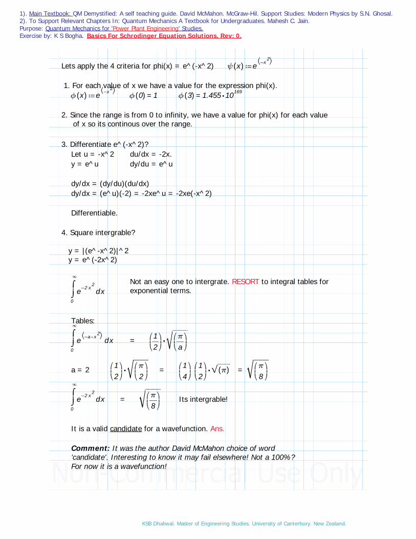
Problem 6.1 (Demystified textbook)
Two functions, psi and phi, be defined for 0<= x < infinity.Explain why psi(x) = x is NOT a wave function but phi(x)=e^(-x^2) is a wave function.Don't be let down by this somewhat simple looking example!
Solution:From your textbook there are 4 criteria to meet this requirement:1. single valued2. continous over the range3. differentiable4. square intergrable ..... read this as shown below.
⌠⎮⌡ d−∞
∞
||ψ((x))||2
x < ∞
Lets apply the 4 criteria for psi(x) = x≔ψ((x)) x
1. For each value of x we have a value for the expression psi(x).A single-valued function is function that, for each point in the domain, has a unique value in the range. It is therefore one-to-one or many-to-one.
2. Since the range is from 0 to infinity, we have a value for psi(x) for each x its continous over the range.3. Differentiate x? d(x)/dx = 1. Differentiable. Its a constant. Met the first 3 criteria.4. Square intergrable? x --> x^2
=⌠⌡ d0
3
x2 x 9 If the upper limit was 3 we have an answer its square intergrable, but our problem is upper limit is infinity not 3.
⌠⎮⌡ d−∞
∞
||ψ((x))||2
x < ∞ If the function is positive --> valued, then limits are 0 to +infinty.
⌠⎮⌡ d0
∞
||ψ((x))||2
x < ∞
⌠⌡ d0
∞
⎛⎝x2⎞⎠ x < ∞ ⋅⎛⎜⎝―13⎞⎟⎠
x3 Limits 0 --> infinity
Result of intergration: (1/3)x^3.When x = infinity, (1/3)(infinity)^3 = infinity.When x = 0, result = 0.Infinity - 0 = Infinity. This is not less than Infinity.So fail.
It is NOT a wave function. Ans.
Solution continued on next page.
KSB Dhaliwal. Master of Engineering Studies. University of Canterbury. New Zealand.
1). Main Textbook: QM Demystified: A self teaching guide. David McMahon. McGraw-Hil. Support Studies: Modern Physics by S.N. Ghosal. 2). To Support Relevant Chapters In: Quantum Mechanics A Textbook for Undergraduates. Mahesh C. Jain. Purpose: Quantum Mechanics for 'Power Plant Engineering' Studies. Exercise by: K S Bogha. Basics For Schrodinger Equation Solutions. Rev: 0.
Lets apply the 4 criteria for phi(x) = e^(-x^2) ≔ψ((x)) e⎛⎝−x
2⎞⎠
1. For each value of x we have a value for the expression phi(x).≔ϕ((x)) e⎛⎝−x
2⎞⎠=ϕ((0)) 1 =ϕ((3)) ⋅1.455 10169
2. Since the range is from 0 to infinity, we have a value for phi(x) for each value of x so its continous over the range.
3. Differentiate e^(-x^2)? Let u = -x^2 du/dx = -2x.y = e^u dy/du = e^u
dy/dx = (dy/du)(du/dx)dy/dx = (e^u)(-2) = -2xe^u = -2xe(-x^2)
Differentiable.
4. Square intergrable?
y = |(e^-x^2)|^2 y = e^(-2x^2)
Not an easy one to intergrate. RESORT to integral tables for exponential terms.
⌠⎮⌡ d0
∞
e−2 x2
x
Tables:⌠⎮⌡ d0
∞
e⎛⎝ ⋅−a x
2⎞⎠x = ⋅⎛
⎜⎝―12⎞⎟⎠‾‾‾‾⎛⎜⎝―πa⎞⎟⎠
a = 2 ⋅⎛⎜⎝―12⎞⎟⎠‾‾‾‾⎛⎜⎝―π2⎞⎟⎠
= ⋅⎛⎜⎝―14⎞⎟⎠⎛⎜⎝―12⎞⎟⎠‾‾‾((π)) =
‾‾‾‾⎛⎜⎝―π8⎞⎟⎠
⌠⎮⌡ d0
∞
e−2 x2
x =‾‾‾‾⎛⎜⎝―π8⎞⎟⎠
Its intergrable!
It is a valid candidate for a wavefunction. Ans.
Comment: It was the author David McMahon choice of word 'candidate'. Interesting to know it may fail elsewhere! Not a 100%?For now it is a wavefunction!
KSB Dhaliwal. Master of Engineering Studies. University of Canterbury. New Zealand.

1). Main Textbook: QM Demystified: A self teaching guide. David McMahon. McGraw-Hil. Support Studies: Modern Physics by S.N. Ghosal. 2). To Support Relevant Chapters In: Quantum Mechanics A Textbook for Undergraduates. Mahesh C. Jain. Purpose: Quantum Mechanics for 'Power Plant Engineering' Studies. Exercise by: K S Bogha. Basics For Schrodinger Equation Solutions. Rev: 0.
Plot of the wave function of the integral of y = e^(-x^2) for a small range.
4⋅10²
6⋅10²
8⋅10²
1⋅10³
1.2⋅10³
1.4⋅10³
1.6⋅10³
1.8⋅10³
0
2⋅10²
2⋅10³
2⋅10⁻¹3⋅10⁻¹4⋅10⁻¹5⋅10⁻¹6⋅10⁻¹7⋅10⁻¹8⋅10⁻¹9⋅10⁻¹0 1⋅10⁻¹ 1x
e−x2
cls ((x))
The purpose of the example problem was to show how to determine whether the function may be a wave function. A good starter example problem.
Took me almost for ever, almost infinty, till I got the integral table for exponential terms!
KSB Dhaliwal. Master of Engineering Studies. University of Canterbury. New Zealand.

1). Main Textbook: QM Demystified: A self teaching guide. David McMahon. McGraw-Hil. Support Studies: Modern Physics by S.N. Ghosal. 2). To Support Relevant Chapters In: Quantum Mechanics A Textbook for Undergraduates. Mahesh C. Jain. Purpose: Quantum Mechanics for 'Power Plant Engineering' Studies. Exercise by: K S Bogha. Basics For Schrodinger Equation Solutions. Rev: 0.
Problem 6.2 (Demystified textbook)
Consider a particle trapped in a well with potential given by:
V(x) = 0 when 0<= x <= aV(x) = infinity when otherwise
Show that PSI(x,t) = A sin(kx) exp(i Et / h') solved the Schrodinger equationprovided that E = (h'^2 k^2) / (2m)Solution:≔Ψ 1 ≔x 1 ≔t 1 ≔E 1 <--So you may not see the red rectangle.
Comment:
This may change from problem to problem, but what is the purpose of the Schrodinger Equation?Quantities, (example the position, momentum, velocities,....etc), of the particle (electron, neutron, proton,....etc), which appear in the old quantum theory cannot be precisely determined because of the uncertainty principle, and hence cannot describe the behaviour of the atomic system.
That appears to be the problem, so what was the solution?
Hisenberg invented the matrix mechanics. This was further improved or developed by Born and Jordan. Soon afterwards Erwin Schrodinger developed the wave mechanics on the basis of DeBroglie's hypothesis of wave-particle duality, and proposed a wave equation for describing the motion of atomic systems. - (Ghosal, Modern Physics Vol I).
Figure to the leftserves to assistsin the problem'ssolution.Where the V(x) = 0the potential is lowso the force acting on the particle is negligible compared to where V(x) is very high. See discussion in box. KE as an additon would make it worst.
KSB Dhaliwal. Master of Engineering Studies. University of Canterbury. New Zealand.

1). Main Textbook: QM Demystified: A self teaching guide. David McMahon. McGraw-Hil. Support Studies: Modern Physics by S.N. Ghosal. 2). To Support Relevant Chapters In: Quantum Mechanics A Textbook for Undergraduates. Mahesh C. Jain. Purpose: Quantum Mechanics for 'Power Plant Engineering' Studies. Exercise by: K S Bogha. Basics For Schrodinger Equation Solutions. Rev: 0.
Let PSI (upper case) be the 1 dimensional wave function shown in the terms below:
wave function = Ψ(( ,x t))<-- Ignore the small red rectangles over the variable caused by the text editor in software. Its because the variable was not defined. We are NOT computing merely using the text editor.
≔lhs ⋅i h'⎛⎜⎝― ―d
dt((Ψ(( ,x t))))
⎞⎟⎠
≔rhs_term1 ⋅−⎛⎜⎝― ―h'2
2 m
⎞⎟⎠
⎛⎜⎝― ―d
d
2
x2((Ψ(( ,x t))))
⎞⎟⎠
≔rhs_term2 ⋅V ((x)) Ψ(( ,x t))
The general One Dimensional Schrodinger expression.Note: rhs_term2 is not applicable in this problem.
The one dimensional time-dependent Schrodinger's wave equation is:lhs = rhs_term 1 + rhs_term 2........PSI shown multiplied through.You find the equation in your recommended textbook.
Our problem equation is: lhs = rhs_term 1
≔Ψ(( ,x t)) ⋅A sin (( ⋅k x)) e― ―⋅⋅−i E t
h'
Derivative of the lhs term above w.r.t. t:
⋅i h' ― ―d
dtΨ(( ,x t)) = ⋅⋅⋅i h' ⎛⎜⎝
― ―⋅−i E
h'⎞⎟⎠
⎛⎜⎝ ⋅A sin (( ⋅k x)) e
― ―⋅⋅−i E th'⎞⎟⎠
Since i x -i = -i^2 = -(-1) = 1, above RHS term becomes positive
⋅i h' ― ―d
dtΨ(( ,x t)) = ⋅E
⎛⎜⎝⋅A sin (( ⋅k x)) e
― ―⋅⋅−i E th'⎞⎟⎠= ⋅E Ψ(( ,x t))
Continuing with the derivative of PSI (x,t) w.r.t. x:
― ―d
dtΨ(( ,x t)) = ― ―
d
dx
⎛⎜⎝ ⋅A sin ((kx)) e
― ―⋅⋅−i E th'⎞⎟⎠ = ⋅⋅k A cos ((kx)) e
― ―⋅⋅−i E th'
Now for the rhs_term1 evaluate it:
⋅−⎛⎜⎝― ―h'2
2 m
⎞⎟⎠
⎛⎜⎝― ―d
d
2
x2((Ψ(( ,x t))))
⎞⎟⎠
= −⎛⎜⎝― ―h'2
2 m
⎞⎟⎠
⎛⎜⎜⎝― ―d
d
2
x2
⎛⎜⎝ ⋅⋅⋅k A cos ((kx)) e
― ―⋅⋅−i E th'⎞⎟⎠⎞⎟⎟⎠
KSB Dhaliwal. Master of Engineering Studies. University of Canterbury. New Zealand.

1). Main Textbook: QM Demystified: A self teaching guide. David McMahon. McGraw-Hil. Support Studies: Modern Physics by S.N. Ghosal. 2). To Support Relevant Chapters In: Quantum Mechanics A Textbook for Undergraduates. Mahesh C. Jain. Purpose: Quantum Mechanics for 'Power Plant Engineering' Studies. Exercise by: K S Bogha. Basics For Schrodinger Equation Solutions. Rev: 0.
= −⎛⎜⎝― ―h'2
2 m
⎞⎟⎠
⎛⎜⎝ ⋅⋅⋅−k2 A sin ((kx)) e
― ―⋅⋅−i E th'⎞⎟⎠
=⎛⎜⎝― ―h'2
2 m
⎞⎟⎠
⋅⎛⎝k2⎞⎠⎛⎜⎝ ⋅⋅A sin ((kx)) e
― ―⋅⋅−i E th'⎞⎟⎠
=⎛⎜⎝― ―h'2
2 m
⎞⎟⎠
⋅⎛⎝k2⎞⎠Ψ(( ,x t))
Returning to our earlier expression:lhs = rhs_term1
⋅i h'⎛⎜⎝― ―d
dt((Ψ(( ,x t))))
⎞⎟⎠
= ⋅−⎛⎜⎝― ―h'2
2 m
⎞⎟⎠
⎛⎜⎝― ―d
d
2
x2((Ψ(( ,x t))))
⎞⎟⎠
Now equating both terms results:
⋅E Ψ(( ,x t)) =⎛⎜⎝― ―h'2
2 m
⎞⎟⎠
⋅⎛⎝k2⎞⎠Ψ(( ,x t))
Solving for E by canceling PSI(x,t). Then we say the Schrodinger equation is satisfifed for the given expression for E.
E =⎛⎜⎝― ― ―⋅h'2 k2
2 m
⎞⎟⎠
Ans.
This is what we accomplished:'Showed the WAVE FUNCTION PSI(x,t) = A sin(kx) exp(i Et / h') solved the Schrodinger equation provided E = (h'^2 k^2) / (2m)'
Comments:
Its not 'thinking out of the box'? Phrase you often hear, but getting the boundary set for where V(x) is infinite and 0 was a problem me, and I maybe wrong I see within 0 to a as in the box and elsewhere out. In the box V(x) is zero, and outside infinity. Why is it so difficult to say in the box V(x) = 0, and elsewhere infinite?
KSB Dhaliwal. Master of Engineering Studies. University of Canterbury. New Zealand.

1). Main Textbook: QM Demystified: A self teaching guide. David McMahon. McGraw-Hil. Support Studies: Modern Physics by S.N. Ghosal. 2). To Support Relevant Chapters In: Quantum Mechanics A Textbook for Undergraduates. Mahesh C. Jain. Purpose: Quantum Mechanics for 'Power Plant Engineering' Studies. Exercise by: K S Bogha. Basics For Schrodinger Equation Solutions. Rev: 0.
Problem 6.3 ( QM DeMystified David McMahon )
Suppose PSI(x,t) = A(x - x^3)e^(-iEt/h').
≔Ψ(( ,x t)) ⋅A⎛⎝−x x3⎞⎠e― ―⋅⋅−i E t
h'
Find V(x) such that the Schrodinger equation is satisfied.
Solution:
⋅−⎛⎜⎝― ―h'2
2 m
⎞⎟⎠
⎛⎜⎝― ―d
d
2
x2((Ψ(( ,x t))))
⎞⎟⎠
+ ⋅V ((x)) Ψ(( ,x t)) = ⋅⎛⎜⎝
+― ― ―⎛⎝ ⋅h'2 k2⎞⎠⋅2 m
V ((x))⎞⎟⎠Ψ(( ,x t))
.....Atomic Physics (Ghoshal) page 244, something like this with a slight change here with PSI(x,t) shown instead of just PSI without the variables x, and t. Of course it be in context......
D. McMahon identifies PHI as the spatial part of the PSI(x,t) expression above. Spatial because it only has variable x (space-spatial).
≔Φ((x)) A⎛⎝−x x3⎞⎠
So now ≔Ψ(( ,x t)) ⋅Φ((x)) e― ―⋅⋅−i E t
h'
⋅−⎛⎜⎝― ―h'2
2 m
⎞⎟⎠
⎛⎜⎝― ―d
d
2
x2((Φ((x))))
⎞⎟⎠
+ ⋅V ((x)) Φ((x)) = ⋅((E)) Φ((x)) We use this eq forthe solution.
Above eq 'Separation of space and time in Schrodinger equation: Time independent Schrodinger equation.'
<--- Eq we use in this solution as D McMahon shows, similar found on page 253.
Since V(x) is spatial we do not need to work with the whole PSI(x,t) equation, instead just PHI(x). Something we would never had thought ourselves, to drop part of the expression would be a crime!
KSB Dhaliwal. Master of Engineering Studies. University of Canterbury. New Zealand.

1). Main Textbook: QM Demystified: A self teaching guide. David McMahon. McGraw-Hil. Support Studies: Modern Physics by S.N. Ghosal. 2). To Support Relevant Chapters In: Quantum Mechanics A Textbook for Undergraduates. Mahesh C. Jain. Purpose: Quantum Mechanics for 'Power Plant Engineering' Studies. Exercise by: K S Bogha. Basics For Schrodinger Equation Solutions. Rev: 0.
Lets look at the right had side of the equation E Phi(x)
⋅E Φ((x)) = ⋅E ⎛⎝⋅A ⎛⎝−x x3⎞⎠⎞⎠
What we do next is a few similar derivatives and plugin's to match up the equation of concern. We do this often!
― ―d
d
2
x2((Φ((x)))) ?
― ―d
d
1
x1((Φ((x)))) = −A ⋅⋅A 3 x2
― ―d
d
2
x2((Φ((x)))) = ⋅⋅−A 6 x
Match up expression:
⋅−⎛⎜⎝― ―h'2
2 m
⎞⎟⎠
⎛⎜⎝― ―d
d
2
x2((Φ((x))))
⎞⎟⎠
= ⋅⋅⋅−⎛⎜⎝― ―h'2
2 m
⎞⎟⎠−A 6 x
Now the eq looks like this:
⋅⋅⋅−⎛⎜⎝― ―h'2
2 m
⎞⎟⎠−A 6 x + ⋅V ((x)) A⎛⎝−x x3⎞⎠= ⋅((E)) A⎛⎝−x x3⎞⎠
⋅⋅⋅⎛⎜⎝― ―h'2
2 m
⎞⎟⎠
A 6 x + ⋅V ((x)) A⎛⎝−x x3⎞⎠= ⋅((E)) A⎛⎝−x x3⎞⎠ Change sign.
Let's not place excessive thinking into this we want to solve for V(x) within the definiton of the 'Schrodinger Equation'.
Rearranging:
⋅V ((x)) A⎛⎝−x x3⎞⎠= ⋅((E)) A⎛⎝−x x3⎞⎠ ⋅⋅⋅−⎛⎜⎝― ―h'2
2 m
⎞⎟⎠
A 6 x Divide boty sides byA(x - x^3)
V ((x)) = −E ― ― ― ―⋅⋅
⎛⎜⎝― ―h'2
2 m
⎞⎟⎠
6 x
⎛⎝−x x3⎞⎠= −E ― ― ― ― ―
⋅⋅h'2 6 x
⋅⋅2 m ⎛⎝−x x3⎞⎠Ans.
KSB Dhaliwal. Master of Engineering Studies. University of Canterbury. New Zealand.

1). Main Textbook: QM Demystified: A self teaching guide. David McMahon. McGraw-Hil. Support Studies: Modern Physics by S.N. Ghosal. 2). To Support Relevant Chapters In: Quantum Mechanics A Textbook for Undergraduates. Mahesh C. Jain. Purpose: Quantum Mechanics for 'Power Plant Engineering' Studies. Exercise by: K S Bogha. Basics For Schrodinger Equation Solutions. Rev: 0.
Problem 6.4: Normalising A Wavefunction.Chapter 2 of QM DeMystified (D McMahon).
A wave function for a particle confined to 0<= x <= a in the ground state, was found to be
≔ψ((x)) ⋅A sin⎛⎜⎝― ―⋅π xa⎞⎟⎠
where A is the normalisation constant.
1). Find A?2). Determine the probability that the particle is found in the interval (a/2) <= x <= (3a/4).
Solution:
In electrical engineering you come across normialisation process in signals, and power systems. We find it here in QM and surely in other engineering fields.
Question: Is the process the same?
My answer NO. Why? Because each time I come across it I have forgotten the procedure and have to starts from the beginning. I hope I am not alone, if I am it does trouble me.
Its an important requirement for solving Schrodinger Equation problems. This is a good example to use for reference.
Notes:A wavefunction psi(x,t), space and time, solves a Schrodinger Equation.If this function is multiplied by an undetermined constant A, it becomes A psi(x,t)
⋅A ψ(( ,x t))
Why is it undetermined? You see it in example 6.5, where a solution of a differential equation takes the form:
≔ψ(( ,x t)) +⋅A sin (( ⋅k x)) ⋅B cos (( ⋅k x))
The solution has constant variables/expressions A and B, they need to be solved. So the normilisation process here is one method of doing so. It maybe the only I do not know that for sure, either way we need to solve for the constant expression A and B. Example 6.5 uses the solution here. ⌠⎮⌡ d−∞
∞
|| ⋅A2 ψ(( ,x t))||2
x = 1 ― ―1
A2= ⌠⎮⌡ d−∞
∞
||ψ(( ,x t))||2
x Solve for A.
KSB Dhaliwal. Master of Engineering Studies. University of Canterbury. New Zealand.

1). Main Textbook: QM Demystified: A self teaching guide. David McMahon. McGraw-Hil. Support Studies: Modern Physics by S.N. Ghosal. 2). To Support Relevant Chapters In: Quantum Mechanics A Textbook for Undergraduates. Mahesh C. Jain. Purpose: Quantum Mechanics for 'Power Plant Engineering' Studies. Exercise by: K S Bogha. Basics For Schrodinger Equation Solutions. Rev: 0.
<--- The meaning of this integral expression is that the particle (electron,....neutron,...whatever) is located somewhere within the space of concern with complete certainty.
The limits on our integral will not be from +infinity through - infinity, rather from 'a' through 0 as provided for x. This is where we expect to find the particle!
1). Find A? So lets begin the steps of this normalisation
⌠⎮⌡ d0
a
||ψ(( ,x t))||2
x =⌠⎮⌡
d
0
a
⋅A2 sin2 ⎛⎜⎝― ―⋅π xa⎞⎟⎠
x = A2 ⌠⎮⌡
d
0
a
⋅sin2 ⎛⎜⎝― ―⋅π xa⎞⎟⎠
x
Simple trig identity solves this; sin^2(u) = (1 - cos(2*u))/2 substitute u = (pi x)/2 into the expression.
= A2
⌠⎮⎮⎮⌡
d
0
a
― ― ― ― ― ―−1 ⋅⋅cos 2 ⎛⎜⎝
― ―⋅π xa⎞⎟⎠
2x = ― ―
A2
2
⎛⎜⎜⎜⎝
⌠⎮⌡
d
0
a
−1 ⋅⋅cos 2 ⎛⎜⎝― ―⋅π xa⎞⎟⎠
x⎞⎟⎟⎟⎠
Continued on next page.
KSB Dhaliwal. Master of Engineering Studies. University of Canterbury. New Zealand.
1). Main Textbook: QM Demystified: A self teaching guide. David McMahon. McGraw-Hil. Support Studies: Modern Physics by S.N. Ghosal. 2). To Support Relevant Chapters In: Quantum Mechanics A Textbook for Undergraduates. Mahesh C. Jain. Purpose: Quantum Mechanics for 'Power Plant Engineering' Studies. Exercise by: K S Bogha. Basics For Schrodinger Equation Solutions. Rev: 0.
= ― ―A2
2
⎛⎜⎝⌠⌡ d0
a
1 x⎞⎟⎠
- ― ―A2
2
⎛⎜⎜⎜⎝
⌠⎮⌡
d
0
a
⋅cos ⎛⎜⎝― ― ―
⋅⋅2 π xa⎞⎟⎠
x⎞⎟⎟⎟⎠
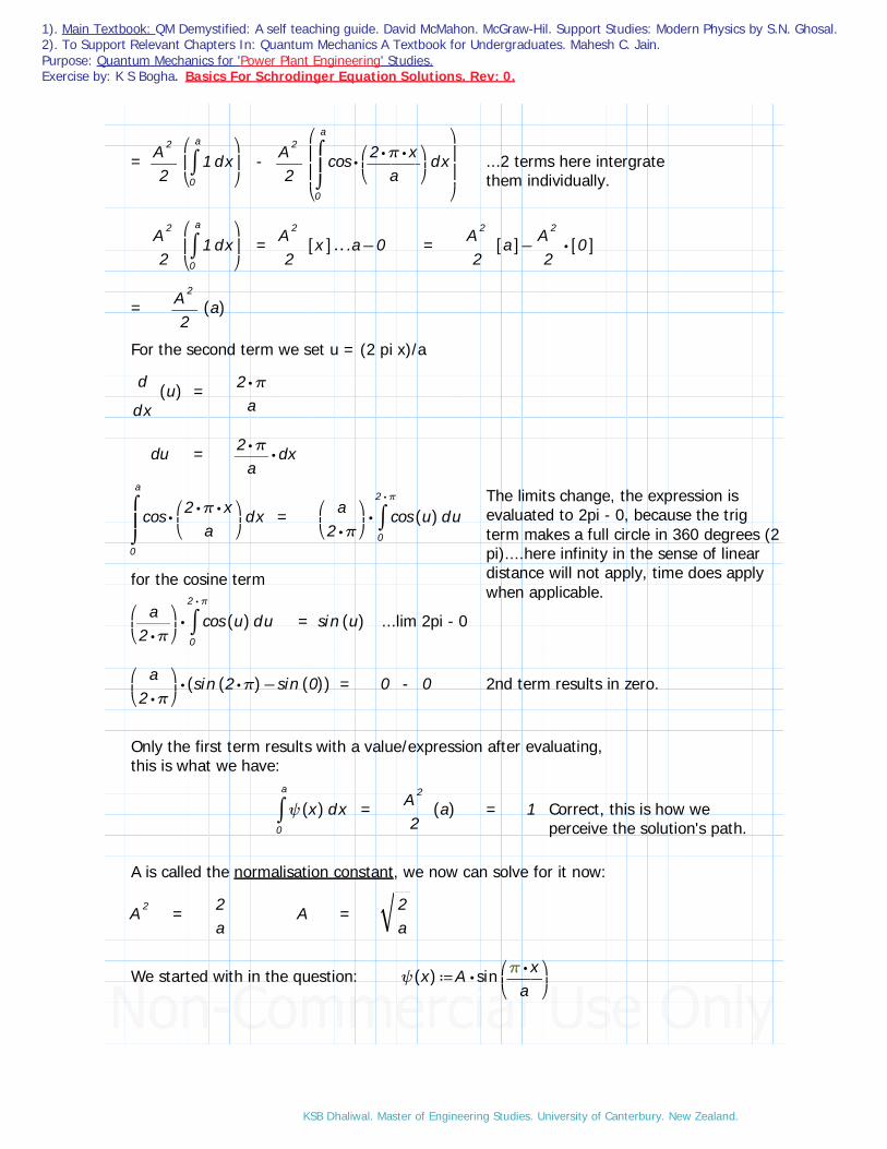
...2 terms here intergrate them individually.
― ―A2
2
⎛⎜⎝⌠⌡ d0
a
1 x⎞⎟⎠
= ‥― ―A2
2x[[ ]] −.a 0 = −― ―
A2
2a[[ ]] ⋅― ―
A2
20[[ ]]
= ― ―A2
2((a))
For the second term we set u = (2 pi x)/a
― ―d
dx((u)) = ― ―
⋅2 πa
du = ⋅― ―⋅2 πa
dx
The limits change, the expression is evaluated to 2pi - 0, because the trig term makes a full circle in 360 degrees (2 pi)....here infinity in the sense of linear distance will not apply, time does apply when applicable.
⌠⎮⌡
d
0
a
⋅cos ⎛⎜⎝― ― ―
⋅⋅2 π xa⎞⎟⎠
x = ⋅⎛⎜⎝― ―
a⋅2 π⎞⎟⎠⌠⌡ d0
⋅2 π
cos ((u)) u
for the cosine term
⋅⎛⎜⎝― ―
a⋅2 π⎞⎟⎠⌠⌡ d0
⋅2 π
cos ((u)) u = sin ((u)) ...lim 2pi - 0
⋅⎛⎜⎝― ―
a⋅2 π⎞⎟⎠
(( −sin (( ⋅2 π)) sin ((0)))) = 0 - 0 2nd term results in zero.
Only the first term results with a value/expression after evaluating, this is what we have:
⌠⌡ d0
a
ψ((x)) x = ― ―A2
2((a)) = 1 Correct, this is how we
perceive the solution's path.
A is called the normalisation constant, we now can solve for it now:
A2 = ―2a
A =‾‾―2a
We started with in the question: ≔ψ((x)) ⋅A sin⎛⎜⎝― ―⋅π xa⎞⎟⎠
KSB Dhaliwal. Master of Engineering Studies. University of Canterbury. New Zealand.

1). Main Textbook: QM Demystified: A self teaching guide. David McMahon. McGraw-Hil. Support Studies: Modern Physics by S.N. Ghosal. 2). To Support Relevant Chapters In: Quantum Mechanics A Textbook for Undergraduates. Mahesh C. Jain. Purpose: Quantum Mechanics for 'Power Plant Engineering' Studies. Exercise by: K S Bogha. Basics For Schrodinger Equation Solutions. Rev: 0.
Substituting in A which was evaluated:
≔ψ((x)) ⋅A sin⎛⎜⎝― ―⋅π xa⎞⎟⎠
The normalised function:
ψ(( ,x t)) = ⋅⎛⎜⎝‾‾―2a
⎞⎟⎠
sin⎛⎜⎝― ―⋅π xa⎞⎟⎠
Ans. The solution to part 1.
2). Determine the probability that the particle is found in the interval
(a/2) <= x <= (3a/4).
In part 1's solution we found the normalisation function and constant. Here we use the function from its original form with it's absolute squared. That is the probability.
P⎛⎜⎝≤≤⎛
⎜⎝―a2⎞⎟⎠
x ⎛⎜⎝― ―3 a
4⎞⎟⎠⎞⎟⎠
=⌠⎮⌡ d
―a2
― ―⋅3 a4
||ψ((x))||2
x =⌠⎮⌡ d
―a2
― ―⋅3 a4
||ψ((x))||2
x
Substituting ≔ψ((x)) ⋅A sin⎛⎜⎝― ―⋅π xa⎞⎟⎠
= ⋅⎛⎜⎝‾‾―2a
⎞⎟⎠
sin⎛⎜⎝― ―⋅π xa⎞⎟⎠
⌠⎮⎮⌡
d
―a2
― ―⋅3 a4
|||
⋅⎛⎜⎝‾‾―2a
⎞⎟⎠
sin⎛⎜⎝― ―⋅π xa⎞⎟⎠
|||
2
x =⌠⎮⌡
d
―a2
― ―⋅3 a4
⋅⎛⎜⎝―2a⎞⎟⎠
sin2 ⎛⎜⎝― ―⋅π xa⎞⎟⎠
x
Its obvious the evaluation we are doing is a little different, the sine term is of the 2nd order.
⎛⎜⎝―2a⎞⎟⎠
⌠⎮⎮⎮⌡
d
―a2
―⋅3 a4
― ― ― ― ― ―−1 ⋅⋅cos 2 ⎛⎜⎝
― ―⋅π xa⎞⎟⎠
2x = ⎛
⎜⎝―1a⎞⎟⎠⌠⌡ d
―a2
―⋅3 a4
1 x - ⎛⎜⎝―1a⎞⎟⎠
⌠⎮⌡
d
―a2
―⋅3 a4
cos⎛⎜⎝― ― ―
⋅⋅2 π xa⎞⎟⎠
x
KSB Dhaliwal. Master of Engineering Studies. University of Canterbury. New Zealand.

1). Main Textbook: QM Demystified: A self teaching guide. David McMahon. McGraw-Hil. Support Studies: Modern Physics by S.N. Ghosal. 2). To Support Relevant Chapters In: Quantum Mechanics A Textbook for Undergraduates. Mahesh C. Jain. Purpose: Quantum Mechanics for 'Power Plant Engineering' Studies. Exercise by: K S Bogha. Basics For Schrodinger Equation Solutions. Rev: 0.
⎛⎜⎝―1a⎞⎟⎠
x[[ ]] - ⋅⋅⎛⎜⎝―1a⎞⎟⎠⎛⎜⎝― ―
a⋅2 π⎞⎟⎠
sin⎛⎜⎝― ― ―
⋅⋅2 π xa⎞⎟⎠
limit (3a/4) to (a/2) limit (3a/4) to (a/2)1st term 2nd term
1st term:
⎛⎜⎝―1a⎞⎟⎠⎛⎜⎝
−― ―3 a
4―a2⎞⎟⎠
= ⎛⎜⎝―1a⎞⎟⎠⎛⎜⎝―a4⎞⎟⎠
= ⎛⎜⎝―14⎞⎟⎠
2nd term:
⋅⋅⎛⎜⎝―1a⎞⎟⎠⎛⎜⎝― ―
a⋅2 π⎞⎟⎠
sin⎛⎜⎝― ― ―
⋅⋅2 π xa⎞⎟⎠
= ⋅−⎛⎜⎝― ―
1⋅2 π⎞⎟⎠
sin⎛⎜⎝― ― ―
⋅⋅2 π xa⎞⎟⎠
limit (3a/4) to (a/2)
+⋅−⎛⎜⎝― ―
1⋅2 π⎞⎟⎠
sin⎛⎜⎝⋅2 π⎛⎜⎝― ―3 a4 a⎞⎟⎠⎞⎟⎠
⋅⎛⎜⎝― ―
1⋅2 π⎞⎟⎠
sin⎛⎜⎝⋅2 π⎛⎜⎝― ―
a2 a⎞⎟⎠⎞⎟⎠
+⋅−⎛⎜⎝― ―
1⋅2 π⎞⎟⎠
sin⎛⎜⎝― ―6 π
4⎞⎟⎠
⋅⎛⎜⎝― ―
1⋅2 π⎞⎟⎠
sin ((π)) = ⋅⎛⎜⎝― ―
1⋅2 π⎞⎟⎠⎛⎜⎝
−sin⎛⎜⎝― ―6 π
4⎞⎟⎠
sin ((π))⎞⎟⎠
⋅−⎛⎜⎝― ―
1⋅2 π⎞⎟⎠⎛⎜⎝
−sin⎛⎜⎝― ―3 π
2⎞⎟⎠
sin ((π))⎞⎟⎠sin ((π)) = 0 in radians
⋅−⎛⎜⎝― ―
1⋅2 π⎞⎟⎠
sin⎛⎜⎝― ―3 π
2⎞⎟⎠
=sin⎛⎜⎝― ―3 π
2⎞⎟⎠−1 in radians
⋅−⎛⎜⎝― ―
1⋅2 π⎞⎟⎠
((−1))
― ―1
2 π
Returning to both parts of the intergral's result
P⎛⎜⎝≤≤⎛
⎜⎝―a2⎞⎟⎠
x ⎛⎜⎝― ―3 a
4⎞⎟⎠⎞⎟⎠
= +⎛⎜⎝―14⎞⎟⎠⎛⎜⎝― ―
12 π⎞⎟⎠
= ― ― ―+4 π 48 π
= ― ―+π 2
4 π
=― ―+π 2
4 π0.409 Ans in radian
Probability is 40.9%? Yes, the unit in radian could return a result anywhere from 0.0 to 1.0. Discuss it with your local engineer.
KSB Dhaliwal. Master of Engineering Studies. University of Canterbury. New Zealand.

1). Main Textbook: QM Demystified: A self teaching guide. David McMahon. McGraw-Hil. Support Studies: Modern Physics by S.N. Ghosal. 2). To Support Relevant Chapters In: Quantum Mechanics A Textbook for Undergraduates. Mahesh C. Jain. Purpose: Quantum Mechanics for 'Power Plant Engineering' Studies. Exercise by: K S Bogha. Basics For Schrodinger Equation Solutions. Rev: 0.
Problem 6.5 (Demystified textbook) Revisiting Problem 6.2
Short introduction. What D McMahon said in QM DeMystefied.
D McMahon: Most of the time, we are given a specific potential and asked to find the form of the wavefunction.
My response: Thats difficult. I prefer just plugin numbers.
D McMahon: ...this involves solving a boundary value problem, process of applying boundary conditions to find a solution to a differential equation.
My response: Differential equations? Thats the separating line! Its a difficult topic for me....LaPlace Tranforms.......all that! Hopefully David is right for your sake because I'm not planning on using them at work or for a hobby.
Problem 6.5Consider a particle trapped in a well with potential given by:
V(x) = 0 when 0<= x <= aV(x) = infinity when otherwise
<-----Usually how you see....but do you notice the boundary conditions? Yes!
Solve the Schrodinger equation for this potential.
Solution:
This figure serves to assist in the solution. If you find something wrong with it, correct it.
KSB Dhaliwal. Master of Engineering Studies. University of Canterbury. New Zealand.
1). Main Textbook: QM Demystified: A self teaching guide. David McMahon. McGraw-Hil. Support Studies: Modern Physics by S.N. Ghosal. 2). To Support Relevant Chapters In: Quantum Mechanics A Textbook for Undergraduates. Mahesh C. Jain. Purpose: Quantum Mechanics for 'Power Plant Engineering' Studies. Exercise by: K S Bogha. Basics For Schrodinger Equation Solutions. Rev: 0.
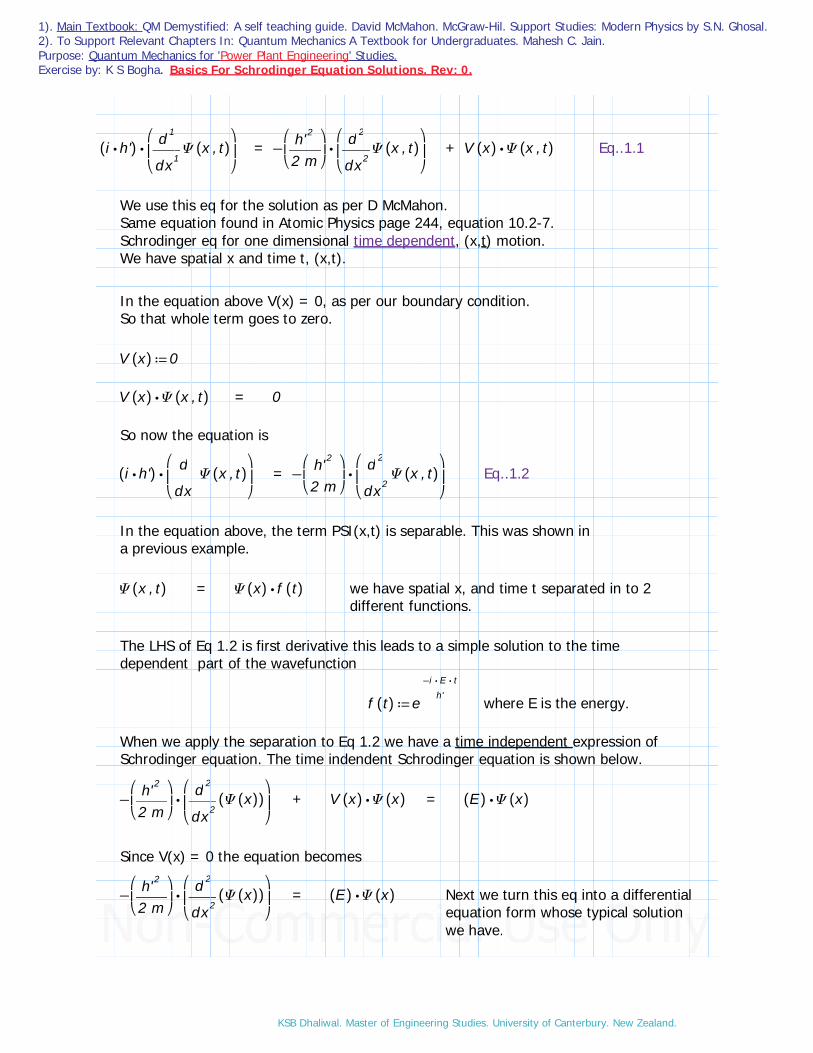
⋅(( ⋅i h'))⎛⎜⎝― ―d
d
1
x1Ψ(( ,x t))
⎞⎟⎠
= ⋅−⎛⎜⎝― ―h'2
2 m
⎞⎟⎠
⎛⎜⎝― ―d
d
2
x2Ψ(( ,x t))
⎞⎟⎠
+ ⋅V ((x)) Ψ(( ,x t)) Eq..1.1
We use this eq for the solution as per D McMahon.Same equation found in Atomic Physics page 244, equation 10.2-7.Schrodinger eq for one dimensional time dependent, (x,t) motion. We have spatial x and time t, (x,t).
In the equation above V(x) = 0, as per our boundary condition.So that whole term goes to zero.
≔V ((x)) 0
⋅V ((x)) Ψ(( ,x t)) = 0
So now the equation is
⋅(( ⋅i h'))⎛⎜⎝― ―
d
dxΨ(( ,x t))
⎞⎟⎠
= ⋅−⎛⎜⎝― ―h'2
2 m
⎞⎟⎠
⎛⎜⎝― ―d
d
2
x2Ψ(( ,x t))
⎞⎟⎠
Eq..1.2
In the equation above, the term PSI(x,t) is separable. This was shown in a previous example.
Ψ(( ,x t)) = ⋅Ψ((x)) f ((t)) we have spatial x, and time t separated in to 2 different functions.
The LHS of Eq 1.2 is first derivative this leads to a simple solution to the time dependent part of the wavefunction
≔f ((t)) e― ―⋅⋅−i E t
h' where E is the energy.
When we apply the separation to Eq 1.2 we have a time independent expression of Schrodinger equation. The time indendent Schrodinger equation is shown below.
⋅−⎛⎜⎝― ―h'2
2 m
⎞⎟⎠
⎛⎜⎝― ―d
d
2
x2((Ψ((x))))
⎞⎟⎠
+ ⋅V ((x)) Ψ((x)) = ⋅((E)) Ψ((x))
Since V(x) = 0 the equation becomes
⋅−⎛⎜⎝― ―h'2
2 m
⎞⎟⎠
⎛⎜⎝― ―d
d
2
x2((Ψ((x))))
⎞⎟⎠
= ⋅((E)) Ψ((x)) Next we turn this eq into a differential equation form whose typical solution we have.
KSB Dhaliwal. Master of Engineering Studies. University of Canterbury. New Zealand.

1). Main Textbook: QM Demystified: A self teaching guide. David McMahon. McGraw-Hil. Support Studies: Modern Physics by S.N. Ghosal. 2). To Support Relevant Chapters In: Quantum Mechanics A Textbook for Undergraduates. Mahesh C. Jain. Purpose: Quantum Mechanics for 'Power Plant Engineering' Studies. Exercise by: K S Bogha. Basics For Schrodinger Equation Solutions. Rev: 0.
So we multiply both sides by ⎛⎜⎝― ―⋅2 m
h'2
⎞⎟⎠
−⎛⎜⎝― ―d
d
2
x2((Ψ((x))))
⎞⎟⎠
+ ⋅⋅⎛⎜⎝― ―⋅2 m
h'2
⎞⎟⎠
((E)) Ψ((x)) = 0 we have a 2nd deritivative equation which needs some simplication.
Let k^2 = (2mE/h'^2) ≔k_squared ― ― ―⋅⋅2 m E
h'2
−⎛⎜⎝― ―d
d
2
x2((Ψ((x))))
⎞⎟⎠
+ ⋅k2 Ψ((x)) = 0 Look up your Diff.Eq. textbook, a solution for this equation is a sinusoidal expression.
Solution for eq above is:
≔Ψ((x)) +⋅A sin (( ⋅k x)) ⋅B cos (( ⋅k x)) Which you may had known or found in the math textbook.
What is the problem now?
We need to solve for A and B in the expression above.
Using the boundary conditions, we apply them to the equation.
We say V(x) is infinite at x=0 and x =a, outside the box. Within the box V(x) = 0.
At x = 0PSI(x=0)--> ≔Ψ((x_equal_Zero)) +⋅A sin (( ⋅k 0)) ⋅B cos (( ⋅k 0))
≔Ψ((x_equal_Zero)) +⋅A sin ((0)) ⋅B cos ((0))≔Ψ((x_equal_Zero)) B
How we interpret this?When B= 0, PSI(0) = A Sin(kx).....Correct!Almost missed that because of the number fixated mind, there is a value thats the answer, sadly this isnt that subject!
≔Ψ((x_equal_zero)) ⋅A sin (( ⋅k x)) Ans. This makes the wave function.
We only used one boundary condition, what I refer to as inside the box,where 0<= x <= a.
What happens at the 'a' side of the boundary?
KSB Dhaliwal. Master of Engineering Studies. University of Canterbury. New Zealand.

1). Main Textbook: QM Demystified: A self teaching guide. David McMahon. McGraw-Hil. Support Studies: Modern Physics by S.N. Ghosal. 2). To Support Relevant Chapters In: Quantum Mechanics A Textbook for Undergraduates. Mahesh C. Jain. Purpose: Quantum Mechanics for 'Power Plant Engineering' Studies. Exercise by: K S Bogha. Basics For Schrodinger Equation Solutions. Rev: 0.
Recall, what we were looking for was the WAVEFUNCTION....and D McMahon said most of the time you will be searching for this function rather than a single numerical value.
A wavefunction like a signal would run thru '0<= x <= a' into the region outside the box. So the wavefunction would require the same result at x=a, as it was for x=0. This wavefunction is expected to be continous everywhere. The solution will satisfy inside the well (box) and outside. Logical!
So, at x=a≔Ψ((x_equal_a)) ⋅A sin (( ⋅k a)) = 0
What is the problem here? How do we make that 0.sin(ka) = 0 ?
Comments: D McMahon says if the wavefunction is ZERO everywhere then there is no particle present in any of the boundary conditions.
You may say if the wavefunction was zero everywhere, to begin with what value had function, but in another way hence there was no particle, for the particle was experiencing that wavefunction's ride to exist in the boundary condition(s). Maybe! .....ride that wave!
To solve the sin(ka) = 0, we apply trignometry and pi.
sin(ka) = 0, what is of concern here is ka.ka = n(pi)n = 1,2,3,.......n cannot equal 0 because sin(0) = 0 !
k = n(pi)/a so now we re-write the wavefunction.
so we dont get any red flag from the software text editor we set n = 1 ≔n 1
≔Ψ((x)) ⋅A sin⎛⎜⎝⋅― ― ―
(( ⋅n π))a
x⎞⎟⎠Ans. ...this is the latest wavefunction which may do it.
Do we need to solve for A? No, its just a 'coefficient or constant or may be a variable' provided in part of the Diff Eq solution's form.
But what about k^2 = 2mE/h'^2....which we set earlier in the steps to the answer?E being the energy of the particle should give some indication of where it is sitting in the boundary, remember the potential is time independent and the solution to the Schrodinger equation was given as:
Ψ(( ,x t)) = ⋅Ψ((x)) f ((t)) ≔f ((t)) e― ―⋅⋅−i E t
h' ⋅Ψ((x)) e― ―⋅⋅−i E t
h'
KSB Dhaliwal. Master of Engineering Studies. University of Canterbury. New Zealand.

1). Main Textbook: QM Demystified: A self teaching guide. David McMahon. McGraw-Hil. Support Studies: Modern Physics by S.N. Ghosal. 2). To Support Relevant Chapters In: Quantum Mechanics A Textbook for Undergraduates. Mahesh C. Jain. Purpose: Quantum Mechanics for 'Power Plant Engineering' Studies. Exercise by: K S Bogha. Basics For Schrodinger Equation Solutions. Rev: 0.
So, maybe E has a role in the solution.
However, 'A' may be solved in the 'Schrodinger Normalisation' OR 'Normalising the Wavefunction' process which is more a mathematical procedure. Which you may have seen in the previous examples, this will be attended to later. At this stage we are more concerned in the Energy (E) role in the solution.
≔k_squared ― ― ―⋅⋅2 m E
h'2
≔E ― ― ―⋅k2 ⎛⎝h'2⎞⎠⋅2 m
simple enough now substitute for k
≔E ― ― ― ― ―⋅⎛⎝ ⋅n2 π2⎞⎠⎛⎝h'2⎞⎠
⋅⋅2 m a2Ans. Solves the energy related to the wavefunction for n = 1, 2, 3,......
Logically n cannot equal 0 because E would result in 0. No Energy.The first value n can assume is n = 1.n=1 is the lowest energy state which you identify as the 'ground state energy'.
We may be able to generate some plots with the results achieved thus far.by setting n=1,2,3.... and mass m of an electron.
Constants:≔h ⋅6.63 10−34 Js =melectron ⋅9.1 10−31
≔h' =― ―h
2 π⋅1.055 10−34
'a' can take on any positive value.....its the distance in reference to 0 in the box or well.
Here we set a = 3, as it was by McMahon in his example.
n values take on a change in the plots.
≔E1 =― ― ― ― ―⋅⎛⎝ ⋅12 π2⎞⎠⎛⎝h'2⎞⎠
⋅⋅2 melectron 32⋅6.709 10−39 when n = 1
≔E2 =― ― ― ― ―⋅⎛⎝ ⋅22 π2⎞⎠⎛⎝h'2⎞⎠
⋅⋅2 melectron 32⋅2.684 10−38 when n = 2
≔E3 =― ― ― ― ―⋅⎛⎝ ⋅32 π2⎞⎠⎛⎝h'2⎞⎠
⋅⋅2 melectron 32⋅6.038 10−38 when n = 3
KSB Dhaliwal. Master of Engineering Studies. University of Canterbury. New Zealand.

1). Main Textbook: QM Demystified: A self teaching guide. David McMahon. McGraw-Hil. Support Studies: Modern Physics by S.N. Ghosal. 2). To Support Relevant Chapters In: Quantum Mechanics A Textbook for Undergraduates. Mahesh C. Jain. Purpose: Quantum Mechanics for 'Power Plant Engineering' Studies. Exercise by: K S Bogha. Basics For Schrodinger Equation Solutions. Rev: 0.
≔Ψ((x)) ⋅A sin⎛⎜⎝⋅― ― ―
(( ⋅n π))a
x⎞⎟⎠We set n = 1,2, and 3 and a = 3for the plots, with x taking on a range 0 - 1, and 1 - 1.
Plot 1: n = 1, a = 3.Plot 2: n = 2, a = 3.Plot 3: n = 3, a = 3.Plot 4: Is probability density of plot 3, |Psi(x)|^2.Graphs using Excel. Matching d McMahon pages 22-23.
Conclusion from plot 4: The particle is nost likely to be found at x = 0.5, 1.5, and 2.5 where the plot peaks at 1. Leat likely to be found at x = 1, and 2 where it peaks at 0. Ans.
Graph of all 4 plots above.
Next page has the graph before the maximisation was conducted. Or in other words normalisation to the maximum value. Just so you get the reasoning behind how I managed to get these plots peaked to 1.
If you got a better way please send it on. The plots are similar to the plots D McMahon provided, of course he is correct. But 'the steps or how to' on how the plots were done on page 22-23 are not given.
KSB Dhaliwal. Master of Engineering Studies. University of Canterbury. New Zealand.

1). Main Textbook: QM Demystified: A self teaching guide. David McMahon. McGraw-Hil. Support Studies: Modern Physics by S.N. Ghosal. 2). To Support Relevant Chapters In: Quantum Mechanics A Textbook for Undergraduates. Mahesh C. Jain. Purpose: Quantum Mechanics for 'Power Plant Engineering' Studies. Exercise by: K S Bogha. Basics For Schrodinger Equation Solutions. Rev: 0.
As you can see these plots do not peak to 1 or -1, they peak to their respective unadjusted maximum values.
Comments:
Good example.
If youre NEW to the engineering business, graphs, data, reports,....are usually fixed to the direction which favours the outcome of a decision to be made by others. Similarly for sign-off papers. This is NOT new.
You read it in countless news reporting on mainstream, or alternative news on the internet. Hence, that is why I showed the adjusted and followed by the first form of the graphs. You are welcome.
If this sounds like a joke you may want to consider taking up applied science for a career instead of engineering.
KSB Dhaliwal. Master of Engineering Studies. University of Canterbury. New Zealand.

1). Main Textbook: QM Demystified: A self teaching guide. David McMahon. McGraw-Hil. Support Studies: Modern Physics by S.N. Ghosal. 2). To Support Relevant Chapters In: Quantum Mechanics A Textbook for Undergraduates. Mahesh C. Jain. Purpose: Quantum Mechanics for 'Power Plant Engineering' Studies. Exercise by: K S Bogha. Basics For Schrodinger Equation Solutions. Rev: 0.
Problem 6.6 (Aruldhas QM Problems With Solution Textbook)Consider the wave function
Again same for the red rectangle ignore the rectangle, same elsewhere.≔Ψ((x)) ⋅⋅A e
⎛⎜⎝― ―−x
2
a2
⎞⎟⎠
e(( ⋅⋅i k x))
≔a 1 By doing this, set a = 1, the software knows the variable a is assigned, it will not impact the solution here since we only use the text editor side of the software.
≔Ψ((x)) ⋅⋅A e
⎛⎜⎝― ―−x
2
a2
⎞⎟⎠
e(( ⋅⋅i k x))
rewritten for clarity PSI(x) = A e ^ (-x^2/a^2) e ^(i k x)Where A is a real constant. 1). Find the value of A ?2). Calculate <p> for this wave function?
Solution:1).
First step here is to normalise the expression, multiply it by its conjugate.
≔Ψconjugate_((x)) ⋅⋅A e
⎛⎜⎝― ―−x
2
a2
⎞⎟⎠
e(( ⋅⋅−i k x)) negative sign in the 2nd exponential term
≔Ψ_Ψconjugate((x)) ⋅A2 e
⎛⎜⎝― ―−2 x
2
a2
⎞⎟⎠
= 1 exponential terms (ikx) results in e^0 = 1.
Next intergrate the expression above shown below:
⋅A2
⌠⎮⎮⌡ de
⎛⎜⎝― ―−2 x
2
a2
⎞⎟⎠
x = 1
<--- From table of exponential integrals.
in the form above, the constant term a: 2/a^2e
⋅⎛⎝((2))⎛⎝―1a
2⎞⎠⎞⎠⎛⎝−x
2⎞⎠
⋅⋅A2 ⎛⎜⎝―12⎞⎟⎠
((2)) ⎛⎜⎜⎝
― ―π
―2
a2
⎞⎟⎟⎠
―12
= 1 ⋅A2 ⎛⎜⎝―π2⎞⎟⎠
―12
= a ≔A⎛⎜⎝‾‾‾‾⎛⎜⎝―2π⎞⎟⎠
⎞⎟⎠
a Ans.
Please verify using your integral tables or manual calculation, thats the textbook answer.
KSB Dhaliwal. Master of Engineering Studies. University of Canterbury. New Zealand.

1). Main Textbook: QM Demystified: A self teaching guide. David McMahon. McGraw-Hil. Support Studies: Modern Physics by S.N. Ghosal. 2). To Support Relevant Chapters In: Quantum Mechanics A Textbook for Undergraduates. Mahesh C. Jain. Purpose: Quantum Mechanics for 'Power Plant Engineering' Studies. Exercise by: K S Bogha. Basics For Schrodinger Equation Solutions. Rev: 0.
2).
Momentum P Hamiltonian operator: ⋅i h'
<-- That is the Laplacian operator. Sine we do not have it in this software in this edition we will use the up pointed triangle usually used for delta.
Comment : This problem is the type you have the solution and so you work backward to make the question. Youre a scientist, engineer,....you know these things, you got the solution in mind, the math to show the reasoning-logic, so you work backward to generate the question. Nothing unusual about creating problems, the real world works like this too. This is NOT reverse eengineering thats something else.
This is a one dimensional case so the expression is: = ⋅⎛⎜⎝―h'i⎞⎟⎠― ―
d
dx
In this problem we use the 2nd form = ⋅(( ⋅−i h')) ― ―d
dxWe work with the 'operator' working on the normalised expression.With Schrodinger appling Normilisation technique is more the norm than exception. One postulate for Schrodinger Equation is just that on Normalisation equal Unity.
⌠⎮⌡
d
0
∞
⋅Ψ_conj⎛⎜⎝⋅−i h'⎛⎜⎝― ―dΨdx⎞⎟⎠⎞⎟⎠
x This is solution it requires setting up the integrals. We use expressions from the first part of the example problem in the solution.
⋅
⎛⎜⎝ ⋅⋅A e
⎛⎜⎝― ―−x
2
a2
⎞⎟⎠
e(( ⋅⋅−i k x))⎞⎟⎠⎛⎜⎝
⋅−i h'⎛⎜⎝― ―dΨdx⎞⎟⎠⎞⎟⎠
First term Second term
Start with the second term, the term to be differentiated:
⎛⎜⎝⋅−i h'⎛⎜⎝― ―dΨdx⎞⎟⎠⎞⎟⎠
= ?
―d
dx
⎛⎜⎝ ⋅⋅A e
⎛⎜⎝― ―−x
2
a2
⎞⎟⎠
e(( ⋅⋅i k x))⎞⎟⎠ = ⋅⋅(( ⋅−i h')) A
⎛⎜⎜⎝
+⋅⎛⎜⎝― ―⋅−2 x
a2
⎞⎟⎠
e
⎛⎜⎝― ―−x
2
a2
⎞⎟⎠
e(( ⋅⋅i k x)) ⋅e
⎛⎜⎝― ―−x
2
a2
⎞⎟⎠
(( ⋅i k)) e(( ⋅⋅i k x))⎞⎟⎟⎠
= ⋅⋅⋅(( ⋅−i h')) A ⎛⎝e ⋅⋅i j k⎞⎠
⎛⎜⎜⎝
+⋅⎛⎜⎝― ―⋅−2 x
a2
⎞⎟⎠
e
⎛⎜⎝― ―−x
2
a2
⎞⎟⎠
⋅e
⎛⎜⎝― ―−x
2
a2
⎞⎟⎠
(( ⋅i k))
⎞⎟⎟⎠
KSB Dhaliwal. Master of Engineering Studies. University of Canterbury. New Zealand.

1). Main Textbook: QM Demystified: A self teaching guide. David McMahon. McGraw-Hil. Support Studies: Modern Physics by S.N. Ghosal. 2). To Support Relevant Chapters In: Quantum Mechanics A Textbook for Undergraduates. Mahesh C. Jain. Purpose: Quantum Mechanics for 'Power Plant Engineering' Studies. Exercise by: K S Bogha. Basics For Schrodinger Equation Solutions. Rev: 0.
Combining the terms:
⋅
⎛⎜⎝ ⋅⋅A e
⎛⎜⎝― ―−x
2
a2
⎞⎟⎠
e(( ⋅⋅−i k x))⎞⎟⎠
⎛⎜⎜⎝
⋅⋅⋅(( ⋅−i h')) A ⎛⎝e ⋅⋅i j k⎞⎠
⎛⎜⎜⎝
+⋅⎛⎜⎝― ―⋅−2 x
a2
⎞⎟⎠
e
⎛⎜⎝― ―−x
2
a2
⎞⎟⎠
⋅e
⎛⎜⎝― ―−x
2
a2
⎞⎟⎠
(( ⋅i k))
⎞⎟⎟⎠
⎞⎟⎟⎠
Expand, evaluate, and place the integral sign:
+⋅⋅⋅⋅⋅(( ⋅−i h')) A2 e
⎛⎜⎝
⋅−2 ―x2
a2
⎞⎟⎠
((1)) ⎛⎜⎝― ―−2
a2
⎞⎟⎠
((x)) ⋅⋅⋅(( ⋅−i h')) A2 e
⎛⎜⎝
⋅−2 ―x2
a2
⎞⎟⎠
(( ⋅i k))
Rearranging:
⋅⋅⋅(( ⋅−i h')) ⎛⎜⎝― ―−2
a2
⎞⎟⎠
A2
⌠⎮⎮⌡ d−∞
∞
⋅e
⎛⎜⎝
⋅−2 ―x2
a2
⎞⎟⎠
((x)) x + ⋅⋅⋅(( ⋅−i h')) (( ⋅i k)) A2
⌠⎮⎮⌡ d−∞
∞
e
⎛⎜⎝
⋅−2 ―x2
a2
⎞⎟⎠
x
The first integral term has an odd term x dx, (x^1) dx, this integral vanishes from -infinity to + infinity. Check your college engineering mathematics textbook for intergration of exponential terms from -infinity to + infinity. Yet a good example with this difficulty on the odd term.
⋅A2
⌠⎮⎮⌡ d−∞
∞
⋅e
⎛⎜⎝― ―−2 x
2
a2
⎞⎟⎠
((x)) x = 1, leaving the right hand side term to:
⋅(( ⋅−i h')) (( ⋅i k)) = ⋅⎛⎝−i2⎞⎠(( ⋅h' k))
Therefore <p> = ⋅h' k Ans.Comments: Took almost a life time of some species to solve this. Reason for this was the expression below required to be corrected, there were 2 wave functions and the differential term so that totalled to 3 terms, INSTEAD of 1 conjugate wave function and the other the wave fuction to be differentated, which was 2 terms shown below.
⌠⎮⌡
d
0
∞
⋅Ψ_conj⎛⎜⎝⋅−i h'⎛⎜⎝― ―dΨdx⎞⎟⎠⎞⎟⎠
x
Advice: Thousands of examples/problems can be given on QM Normalisation. There is no endto them. Here we got the general idea thru a few simple examples. Easy ones, sophisticated ones, oh beautiful/elegant ones, and very lengthty ones there are, so there is NO point in going further. No end to the beauty and elegance of mathematical expressions!
KSB Dhaliwal. Master of Engineering Studies. University of Canterbury. New Zealand.
1). Main Textbook: QM Demystified: A self teaching guide. David McMahon. McGraw-Hil. Support Studies: Modern Physics by S.N. Ghosal. 2). To Support Relevant Chapters In: Quantum Mechanics A Textbook for Undergraduates. Mahesh C. Jain. Purpose: Quantum Mechanics for 'Power Plant Engineering' Studies. Exercise by: K S Bogha. Basics For Schrodinger Equation Solutions. Rev: 0.
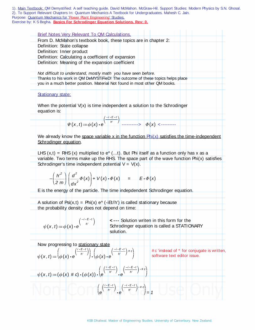
Brief Notes Very Relevant To QM Calculations.From D. McMahon's textbook book, these topics are in chapter 2: Definition: State collapseDefinition: Inner productDefinition: Calculating a coefficient of expansionDefinition: Meaning of the expansion coefficient
Not difficult to understand, mostly math you have seen before. Thanks to his work in QM DeMYSTiFieD! The outcome of these topics helps place you in a much better position. Material Not found in most other QM books.
Stationary state:
When the potential V(x) is time independent a solution to the Schrodinger equation is:
≔Ψ(( ,x t)) ⋅ϕ((x)) e⎛⎝― ―⋅⋅−i E t
h'⎞⎠
----------> Φ((x)) <---------
We already know the space variable x in the function Phi(x) satisfies the time-independent Schrodinger equation.
LHS (x,t) = RHS (x) multiplied to e^(...t). But Phi itself as a function only has x as a variable. Two terms make up the RHS. The space part of the wave function Phi(x) satisfies Schrodinger's time independent potential V = V(x).
+−⎛⎜⎝― ―h'2
2 m
⎞⎟⎠
⎛⎜⎝― ―d
d
2
x2Φ((x))
⎞⎟⎠
⋅V ((x)) Φ((x)) = ⋅E Φ((x))
E is the energy of the particle. The time indepdendent Schrodinger equation.
A solution of Psi(x,t) = Phi(x) e^(-iEt/h') is called stationary becausethe probability density does not depend on time:
<--- Solution writen in this form for the Schrodinger equation is called a STATIONARY solution.
≔ψ(( ,x t)) ⋅ϕ((x)) e⎛⎝― ―
⋅⋅−i E th'⎞⎠
Now progressing to stationary state#c 'instead of * for conjugate is written, software text editor issue.≔ψ(( ,x t)) ⋅
⎛⎜⎝ ⋅ϕ((x)) e
⎛⎝― ―⋅⋅i E t
h'⎞⎠⎞⎟⎠⎛⎜⎝ ⋅ϕ((x)) e
⎛⎝― ―⋅⋅−i E t
h'⎞⎠#c⎞⎟⎠
≔ψ(( ,x t)) ⋅⋅((ϕ((x)) #c)) ((ϕ((x))))⎛⎜⎝ ⋅e⎛⎝― ―
⋅⋅i E th'⎞⎠
e⋅⎛⎝― ―
⋅⋅−i E th'⎞⎠#c⎞⎟⎠
=⎛⎜⎝ ⋅e⎛⎝― ―
⋅⋅i E th'⎞⎠
e⋅⎛⎝― ―
⋅⋅−i E th'⎞⎠#c⎞⎟⎠ 1
KSB Dhaliwal. Master of Engineering Studies. University of Canterbury. New Zealand.

1). Main Textbook: QM Demystified: A self teaching guide. David McMahon. McGraw-Hil. Support Studies: Modern Physics by S.N. Ghosal. 2). To Support Relevant Chapters In: Quantum Mechanics A Textbook for Undergraduates. Mahesh C. Jain. Purpose: Quantum Mechanics for 'Power Plant Engineering' Studies. Exercise by: K S Bogha. Basics For Schrodinger Equation Solutions. Rev: 0.
≔ψ(( ,x t)) ⋅((ϕ((x)) #c)) ((ϕ((x)))) So, the function is spatial-space dependent and NOT time. Its called the stationary state. This seen in the previous example problems in the functions with variable x, Psi(x), when solving Schrodinger equation.
Superposition of stationary states:
Consider the superposition of stationary states Psi1(x,t), Psi2(x,t),.....Psi_n_(x,t)ψ1(( ,x t)) ψ2(( ,x t)) ψ3(( ,x t)) ψn (( ,x t))
Above states are solutions of the Schrodinger equation for a given potential V(x). These stationary states can be writen as:
≔ψn (( ,x t)) ⋅ϕn ((x)) e⎛⎝― ―
⋅⋅−i E th'⎞⎠
When can we combine the stationary states? At a given time, that is the same time for all of the states, could be any time, but that they are moving, NOT stationary, so it has to be at time t = 0? No, a particle may come to rest at time(s) other than t=0, i.e. when its back to its ground state or non-excited state. Basically we are trying to say at t=0 is particle is stationary.
At time t = 0 any wave function Psi(x,0) can be writen as a combination of these states:
ψ(( ,x 0)) = ∑ Cnϕn ((x)) OR writen in full ∑ ⋅Cnϕn ((x)) e⎛⎝― ―
⋅⋅−i E th'⎞⎠
Really nothing speical so far just adding them up, and thats called superposition BUT Cnis a coefficient! It need solving. So example on this later should make clear.
From previous studies in QM or Physics:
v (freq) = w/2 piE = h w / 2 pi where h/ 2 pi = h'E = h'wtherefore w = E/h'also p = h'k where k is the wave vector.
Substitute w = E/h' and in terms of summation w_n
ψ(( ,x 0)) = ∑ Cnϕn ((x)) ∑ ⋅Cnϕn ((x)) e⎛⎝― ―
⋅⋅−i E th'⎞⎠
= ∑ ⋅Cnϕn ((x)) e(( ⋅⋅−i wn t))
So we see any function Psi(x,t) can be expanded, i.e. summation expression, in terms of Phi_n. All the Phi_n's make up a set of basis functions.
Ψ ---> Φn
KSB Dhaliwal. Master of Engineering Studies. University of Canterbury. New Zealand.

1). Main Textbook: QM Demystified: A self teaching guide. David McMahon. McGraw-Hil. Support Studies: Modern Physics by S.N. Ghosal. 2). To Support Relevant Chapters In: Quantum Mechanics A Textbook for Undergraduates. Mahesh C. Jain. Purpose: Quantum Mechanics for 'Power Plant Engineering' Studies. Exercise by: K S Bogha. Basics For Schrodinger Equation Solutions. Rev: 0.
Example a vector can be split into its x, y, and z components. You remember in the vector unit (i,j,k) so something like this sums up for the vector. NOT exactly the same here, similar. You got the general picture. When you have all the i j k or x y z for a vector in 3D space, you say the function is complete, here Phi_n is complete.
State collapse: Applying superposition.
Given a function, at time t its at a certain state. Nothing new there thats the same for all function wrt to time. At a specific time in QM we may mean state as in energy level ! So a little more specific here in this subject to energy level.
Ψ(( ,x t)) = ∑ ⋅CnΦn ((x)) e ⋅⋅−i wn t
Lets say for the function above at a certain time when a measurement is made and the energy measured, Ei = h'wi.
≔Ei ⋅h' ωiThe state of the system, wrt to energy measured, takes on the state Phi_i_(x) at time of measurement or immediately after. You may say dependent on system behaviour.
measurement record State of SystemΨ(( ,x t)) --------------------------------> EiΦi ((x))
We take another measurement i.e. a 2nd measurement right after the first measurement. The energy is found to be E = h'w_i. This time with certainty, and surely so, its the 2nd time, accuray was a concern.
≔Ei ⋅h' ωi
Both instances the expression is similar, with the subscript i identifying the i-th instance of the energy. Nothing new here.
h' is the same.w_i; w is the angular frequency and i-th instance is the i-th sequence of measurement of E_i.
Nothing to note so far, its like any other engineering function. With the system left alone, the wavefucntion will spread out, as it should its an energy wave. It spread out as per expectation of the expression provided before shown here again with relevance to w_n in the exponential term:
Ψ(( ,x t)) = ∑ ⋅CnΦn ((x)) e ⋅⋅−i wn t
As it spreads out, EXPANDS, it becomes a superposition of states. Key here is states in the phrase superposition of states. NOT superposition of wavefunctions. Got It!To solve the expression above, we need to find Cn.To do this we use the INNER PRODUCT. You seen this in Engineering Mathematics.
KSB Dhaliwal. Master of Engineering Studies. University of Canterbury. New Zealand.

1). Main Textbook: QM Demystified: A self teaching guide. David McMahon. McGraw-Hil. Support Studies: Modern Physics by S.N. Ghosal. 2). To Support Relevant Chapters In: Quantum Mechanics A Textbook for Undergraduates. Mahesh C. Jain. Purpose: Quantum Mechanics for 'Power Plant Engineering' Studies. Exercise by: K S Bogha. Basics For Schrodinger Equation Solutions. Rev: 0.
Inner Product of 2 Wavefunctions.
2 wave functions shown below:Φ(( ,x t)) Ψ(( ,x t))
Their inner product (Phi, Psi):((Φ_Ψ)) = ⌠⌡ d⋅Φ_conjugate((x)) Ψ((x)) x
Square the LHS:((Φ_Ψ))2 =
⎛⎜⎝⌠⌡ d⋅Φ_conjugate((x)) Ψ((x)) x
⎞⎟⎠
2
The result of the above square of (Phi,Psi) gives the probability that a measurement will find the system in state__ Φ((x))given that it was originally in the state__Ψ((x))This does not mean anything untill we see an example later. I don't see how you could understand it now no more than the next person who said so. Sure the meaning is like it was in one state and that operation got it to the next.
Basis states are orthogonal. That is each pair of the basis are orthogonal, at right angles. At right angles the product of the 2 wave functions is 0, provided each basis is not the same as the other.
⌠⌡ d⋅Φm_conjugate ((x)) Ψn ((x)) x = 0 Provided m is NOT equal to n.
Given the number of basis states and all were normalised_Then as above their product is orthonormal.
Φn ((x))
⌠⌡ d⋅Φm_conjugate ((x)) Ψn ((x)) x = 0 ≠m n
if m NOT equal to n.and⌠⌡ d⋅Φm_conjugate ((x)) Ψn ((x)) x = 1 =m n
if m NOT equal to n.The orthonormal relationship can be expressed using the Kronecker delta function:δmn = 0 if ≠m n
1 if =m nWhich is the same as: ⌠
⌡ d⋅Φm_conjugate ((x)) Ψn ((x)) x = δmn
Weldone ! Lets look at an example later.A vector is said to be normal if it has a length of one. Two vectors are said to be orthogonal if they are at right angles to each other (i.e. their dot product equal 0). A set of vectors is said to be orthonormal if they are all normal, and each pair of vectors in the set is said to be orthogonal. <---Please verify.
In linear algebra, two vectors in an inner product space are orthonormal if they areorthogonal and unit vectors. A set of vectors form an orthonormal set if all vectors in the set are mutually orthogonal and all of unit length. An orthonormal set which forms a basis is called an orthonormal basis. <---Please verify. Pulling out your math book and looking it up will help.
KSB Dhaliwal. Master of Engineering Studies. University of Canterbury. New Zealand.

1). Main Textbook: QM Demystified: A self teaching guide. David McMahon. McGraw-Hil. Support Studies: Modern Physics by S.N. Ghosal. 2). To Support Relevant Chapters In: Quantum Mechanics A Textbook for Undergraduates. Mahesh C. Jain. Purpose: Quantum Mechanics for 'Power Plant Engineering' Studies. Exercise by: K S Bogha. Basics For Schrodinger Equation Solutions. Rev: 0.
Calculating a Coefficient of Expansion.
A state ψ(( ,x 0)) is written as a sum of basis functions Φn ((x))the nth coefficient of expansion Cn is found by computing the inner product ofϕn ((x)) with ψ(( ,x 0)) :
Cn = ( ) =ϕn ((x)), ψ(( ,x 0)) ⌠⌡ d⋅Φn_conjugate ((x)) ψ(( ,x 0)) x <---RHS term
Note the variable t = 0, that is interpretated for a time independent Schrodinger equation. Here the spatial zone or area is of concern. Looks like it.
ψ(( ,x 0)) = ∑ ⋅CnΦn ((x)) e ⋅⋅−i wn 0 = ∑ ⋅CnΦn ((x)) ((1)) Looks like this.
Because we have nth for the Psi_n(x) function, so the Psi(x,0) function will have the mth term. Correct? n & m, where n not equal to m.
Lets continue now with the expansion of the RHS term.
⌠⌡ d⋅ϕn_conjugate ((x)) ψ(( ,x 0)) x =
⌠⎮⌡
dϕn_conjugate ((x)) .⎛⎜⎝∑ CmΦm ((x))
⎞⎟⎠
x
= ⋅⎛⎜⎝∑ Cm
⎞⎟⎠⌠⌡ dϕn_conjugate ((x)) .Φm ((x)) x
= ⋅⎛⎜⎝∑ Cm
⎞⎟⎠⌠⌡ d⎛⎝δmn⎞⎠ x
= ∑ Cm⎛⎝δmn⎞⎠
= ∑ Cmδmn d = 1 when m = n, else 0δmn = 0 if ≠m n
1 if =m nwhich leaves the subscript of C be equal n.All the subscripts, m & n, have to be the same for it to equal 1
= ∑ Cnδnn = ∑ Cn ((1)) summation of the one term, the nth term is Cn, not from 1 to Cn, just Cn
= Cn
Emm...so a good example should make good on how to get that Cn. Comments: Next just a minor addition to what we got thus far reaching to Cn. It is quite critical but you got some understanding of it already. If NOT the major critical side of QM....my say so as a non-physicts. It is...what is the expectation of finding a particle or system given the space or region, the expectation in a probability sense. I may be correct!
KSB Dhaliwal. Master of Engineering Studies. University of Canterbury. New Zealand.
1). Main Textbook: QM Demystified: A self teaching guide. David McMahon. McGraw-Hil. Support Studies: Modern Physics by S.N. Ghosal. 2). To Support Relevant Chapters In: Quantum Mechanics A Textbook for Undergraduates. Mahesh C. Jain. Purpose: Quantum Mechanics for 'Power Plant Engineering' Studies. Exercise by: K S Bogha. Basics For Schrodinger Equation Solutions. Rev: 0.
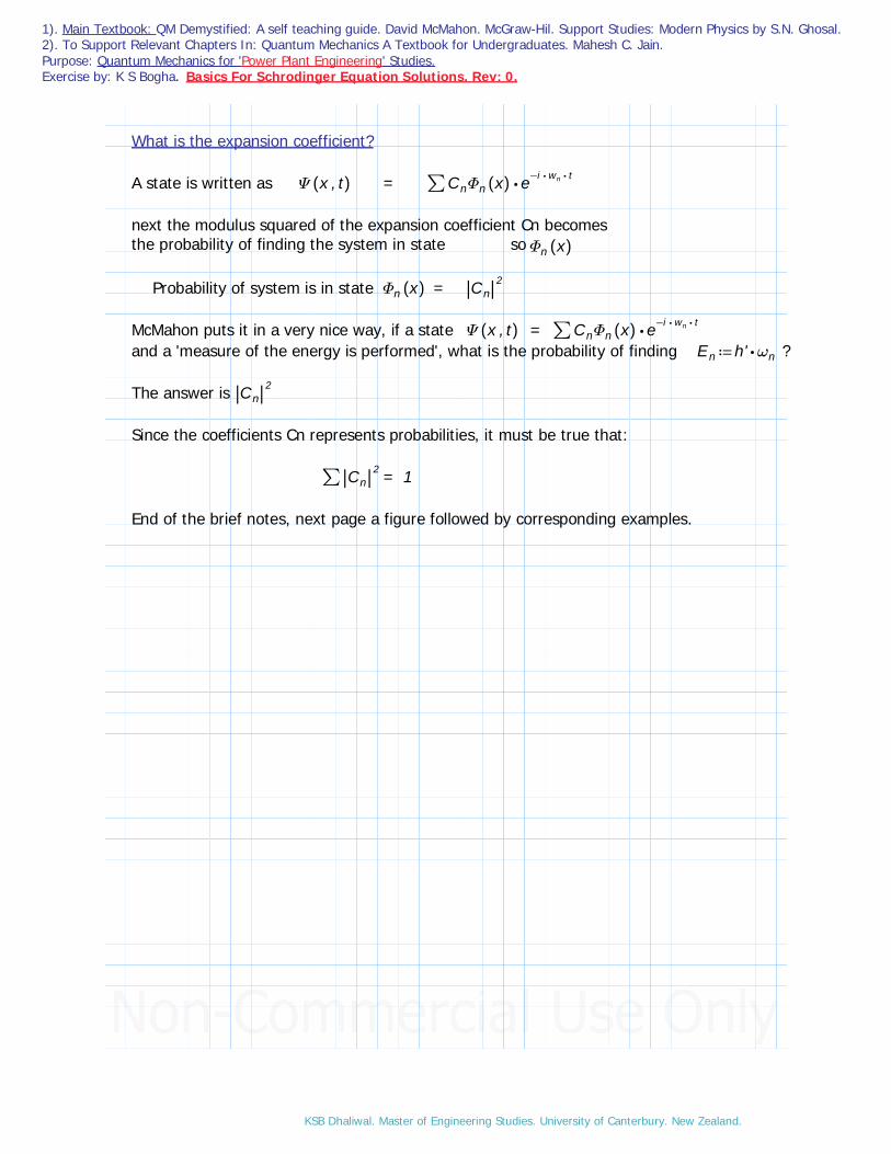
What is the expansion coefficient?
A state is written as Ψ(( ,x t)) = ∑ ⋅CnΦn ((x)) e ⋅⋅−i wn t
next the modulus squared of the expansion coefficient Cn becomes the probability of finding the system in state soΦn ((x))
Probability of system is in state =Φn ((x)) ||Cn||2
McMahon puts it in a very nice way, if a state Ψ(( ,x t)) = ∑ ⋅CnΦn ((x)) e ⋅⋅−i wn t
and a 'measure of the energy is performed', what is the probability of finding ≔En ⋅h' ωn ?
The answer is ||Cn||2
Since the coefficients Cn represents probabilities, it must be true that:
∑ ||Cn||2 = 1
End of the brief notes, next page a figure followed by corresponding examples.
KSB Dhaliwal. Master of Engineering Studies. University of Canterbury. New Zealand.

1). Main Textbook: QM Demystified: A self teaching guide. David McMahon. McGraw-Hil. Support Studies: Modern Physics by S.N. Ghosal. 2). To Support Relevant Chapters In: Quantum Mechanics A Textbook for Undergraduates. Mahesh C. Jain. Purpose: Quantum Mechanics for 'Power Plant Engineering' Studies. Exercise by: K S Bogha. Basics For Schrodinger Equation Solutions. Rev: 0.
Comment: It will not surprise me if you find something wrong in the figure above, my idea, but it will surprise me if its reasonably okay and needing minor corrections!
KSB Dhaliwal. Master of Engineering Studies. University of Canterbury. New Zealand.

1). Main Textbook: QM Demystified: A self teaching guide. David McMahon. McGraw-Hil. Support Studies: Modern Physics by S.N. Ghosal. 2). To Support Relevant Chapters In: Quantum Mechanics A Textbook for Undergraduates. Mahesh C. Jain. Purpose: Quantum Mechanics for 'Power Plant Engineering' Studies. Exercise by: K S Bogha. Basics For Schrodinger Equation Solutions. Rev: 0.
Problem 6.7 (Expansion of the wavefunction and fitting coefficients)QM DeMystified by D McMahon.
A particle of mass m is trapped in a one-dimensional box of width a. The wavefunction is known to be:
≔ψ((x)) −+⋅⋅⎛⎜⎝―i2⎞⎟⎠
⎛⎜⎝‾‾―2a
⎞⎟⎠
sin⎛⎜⎝― ―⋅π xa⎞⎟⎠
⋅⎛⎜⎝‾‾―1a
⎞⎟⎠
sin⎛⎜⎝― ― ―
⋅⋅3 π xa⎞⎟⎠
⋅⋅⎛⎜⎝―12⎞⎟⎠
⎛⎜⎝‾‾―2a
⎞⎟⎠
sin⎛⎜⎝― ― ―⋅4 π x
a⎞⎟⎠
If the energy is measured, what are the possible results and what is the probability of obtaining each result?What is the most probable energy for this state?
Solution:
From the solutions of past 2 examples, we found a normalised wave function that fits the wavefunction above, and also found an expression for En. This function needs to be adjusted, which is done later. Here
≔Φn ((x)) ⋅⎛⎜⎝‾‾―2a
⎞⎟⎠
sin⎛⎜⎝― ― ―
⋅⋅n π xa
⎞⎟⎠
≔En ― ― ― ―⋅n2 h'2 π2
⋅⋅2 m a2
In the problem statement's equation the value of n in (n pi x / a) are n = 1, 3, and 4.So we shall create a table for n = 1 thru 4.
n
1
2
3
4
Φn ((x))
⋅‾‾―2a
sin⎛⎜⎝― ―⋅π x
a⎞⎟⎠
⋅‾‾―2a
sin⎛⎜⎝― ― ―⋅⋅2 π x
a⎞⎟⎠
⋅‾‾―2a
sin⎛⎜⎝― ― ―⋅⋅3 π x
a⎞⎟⎠
⋅‾‾―2a
sin⎛⎜⎝― ― ―⋅⋅4 π x
a⎞⎟⎠
En
― ― ―⋅h'2 π
⋅⋅2 m a2
― ― ―⋅⋅4 h'2 π
⋅⋅2 m a2
― ― ―⋅⋅9 h'2 π
⋅⋅2 m a2
― ― ― ―⋅⋅16 h'2 π
⋅⋅2 m a2
<--- The values of Phi_n(x) in the table, each has (Sqrt(2/a)) multiplied. These terms are not similar to the problem function expression. So we need to make fit so it does match. This by adjusting the wavefunction Psi(x).
KSB Dhaliwal. Master of Engineering Studies. University of Canterbury. New Zealand.

1). Main Textbook: QM Demystified: A self teaching guide. David McMahon. McGraw-Hil. Support Studies: Modern Physics by S.N. Ghosal. 2). To Support Relevant Chapters In: Quantum Mechanics A Textbook for Undergraduates. Mahesh C. Jain. Purpose: Quantum Mechanics for 'Power Plant Engineering' Studies. Exercise by: K S Bogha. Basics For Schrodinger Equation Solutions. Rev: 0.
Multiply by‾‾―22
each of the terms in the function, which you know Sqrt(2/2) =1, and it may only impact the concerned off middle term.
≔ψ((x)) −+⋅⋅⎛⎜⎝―i2⎞⎟⎠
⎛⎜⎝‾‾―2a
⎞⎟⎠
sin⎛⎜⎝― ―⋅π xa⎞⎟⎠
⋅⎛⎜⎝‾‾―22
⎞⎟⎠
⎛⎜⎝‾‾―1a
⎞⎟⎠
sin⎛⎜⎝― ― ―
⋅⋅3 π xa⎞⎟⎠
⋅⋅⎛⎜⎝―12⎞⎟⎠
⎛⎜⎝‾‾―2a
⎞⎟⎠
sin⎛⎜⎝― ― ―⋅4 π x
a⎞⎟⎠
≔ψ((x)) −+⋅⋅⎛⎜⎝―i2⎞⎟⎠
⎛⎜⎝‾‾―2a
⎞⎟⎠
sin⎛⎜⎝― ―⋅π xa⎞⎟⎠
⋅⎛⎜⎝― ―
1
‾‾2
⎞⎟⎠
⎛⎜⎝‾‾―2a
⎞⎟⎠
sin⎛⎜⎝― ― ―
⋅⋅3 π xa⎞⎟⎠
⋅⋅⎛⎜⎝―12⎞⎟⎠
⎛⎜⎝‾‾―2a
⎞⎟⎠
sin⎛⎜⎝― ― ―⋅4 π x
a⎞⎟⎠
Let ≔Φn ((x)) ⋅⎛⎜⎝‾‾―2a
⎞⎟⎠
sin⎛⎜⎝― ― ―
⋅⋅n π xa
⎞⎟⎠
≔ψ((x)) −+⋅⎛⎜⎝―i2⎞⎟⎠Φ1 ((x)) ⎛
⎜⎝― ―
1
‾‾2
⎞⎟⎠Φ3 ((x)) ⋅⎛
⎜⎝―12⎞⎟⎠Φ4 ((x)) Ignore the red rectangle
Look over carefully the expression above.We see a coefficients, (i/2) ..(sqrt(1/2) ..-(1/2), infront of the Phi(x) function across the expression.
That would fit the coefficient of expansion idea we just studied:
≔Ψ((x)) ∑ ⋅Cn Φn ((x)) Ignore the red rectangle
Comment: McMahon creates an updated table to insert Cn....very enigneer like! You can't complaint about D McMahon here. Suggest you pick up his style of work or add to your existing, if youre not already doing it.
n
1
2
3
4
Cn
―i2
0
― ―1
‾‾2
−―12
Φn ((x))
⋅‾‾―2a
sin⎛⎜⎝― ―⋅π x
a⎞⎟⎠
⋅‾‾―2a
sin⎛⎜⎝― ― ―⋅⋅2 π x
a⎞⎟⎠
⋅‾‾―2a
sin⎛⎜⎝― ― ―⋅⋅3 π x
a⎞⎟⎠
⋅‾‾―2a
sin⎛⎜⎝― ― ―
⋅⋅4 π xa⎞⎟⎠
En
― ― ―⋅h'2 π
⋅⋅2 m a2
― ― ―⋅⋅4 h'2 π
⋅⋅2 m a2
― ― ―⋅⋅9 h'2 π
⋅⋅2 m a2
― ― ― ―⋅⋅16 h'2 π
⋅⋅2 m a2
<---Do you see a problem here?C_2: 0.This tells us the energy at n=2 would be zero. Probability of finding anything here is? Zero.We can live with that, its just that our mindset may been tune into a continous case of n =1 thru 4. That's all !
KSB Dhaliwal. Master of Engineering Studies. University of Canterbury. New Zealand.

1). Main Textbook: QM Demystified: A self teaching guide. David McMahon. McGraw-Hil. Support Studies: Modern Physics by S.N. Ghosal. 2). To Support Relevant Chapters In: Quantum Mechanics A Textbook for Undergraduates. Mahesh C. Jain. Purpose: Quantum Mechanics for 'Power Plant Engineering' Studies. Exercise by: K S Bogha. Basics For Schrodinger Equation Solutions. Rev: 0.
1). Answers to part 1.
Now proceed for the computation of the energy, and probability of measuring each energy; for n = 1, 3, and 4.
≔En ― ― ― ―⋅⋅n h'2 π2
⋅⋅2 m a
≔n 1
Note: C1 is an imaginary numer, i, so we take the conjugate for the square.
≔E1 ― ― ― ―⋅1. h'2 π2
⋅⋅2 m aAns ≔P⎛⎝E1⎞⎠ ||C1||
2 ⋅c1_conj c1 = =⋅⎛⎜⎝―−i2⎞⎟⎠⎛⎜⎝―i2⎞⎟⎠
0.25 Ans.
≔n 3 Real number of C3 so we just take the modulus square.
≔E3 ― ― ― ―⋅⋅3 h'2 π2
⋅⋅2 m aAns ≔P⎛⎝E1⎞⎠ ||C3||
2 = =⋅⎛⎜⎝― ―
1
‾‾2
⎞⎟⎠
⎛⎜⎝― ―
1
‾‾2
⎞⎟⎠
0.5 Ans.
≔n 4
≔E4 ― ― ― ―⋅⋅4 h'2 π2
⋅⋅2 m aAns ≔P⎛⎝E1⎞⎠ ||C4||
2 = =⋅⎛⎜⎝−―
12⎞⎟⎠⎛⎜⎝−―
12⎞⎟⎠
0.25 Ans.
All the probabiliies are real numser as should be.
2). Answers to part 2.
From the results above of the probabilities, n = 3 has the highest probability at 50%. Hence, the probable energy for this state is E3
≔E3 ― ― ―⋅⋅9 h'2 π
⋅⋅2 m a2Ans.
Comments:
This was a good example. The difficult part would be on the wavefunction's complexity. Getting the function set in a form that assists the steps for the solution of the coefficients, this would pose for me the tough part.
KSB Dhaliwal. Master of Engineering Studies. University of Canterbury. New Zealand.

1). Main Textbook: QM Demystified: A self teaching guide. David McMahon. McGraw-Hil. Support Studies: Modern Physics by S.N. Ghosal. 2). To Support Relevant Chapters In: Quantum Mechanics A Textbook for Undergraduates. Mahesh C. Jain. Purpose: Quantum Mechanics for 'Power Plant Engineering' Studies. Exercise by: K S Bogha. Basics For Schrodinger Equation Solutions. Rev: 0.
Problem 6. 8 Dot Product & Energy of System after measurement.
A particle in a one-dimensional box (0<= x <= a) as in the state:
≔ψ((x)) ++⋅⎛⎜⎝― ― ―
1
‾‾‾‾⋅10 a
⎞⎟⎠
sin⎛⎜⎝― ―⋅π xa⎞⎟⎠
⋅⋅A⎛⎜⎝‾‾―2a
⎞⎟⎠
sin⎛⎜⎝― ― ―
⋅⋅2 π xa⎞⎟⎠
⋅⎛⎜⎝― ― ―
3
‾‾‾‾⋅5 a
⎞⎟⎠
sin⎛⎜⎝― ― ―⋅3 π x
a⎞⎟⎠
1). Find A so that ψ((x)) is normalised.2). What are the possible results of measurements of the energy, and what are the respective probabilities of obtaining each result?3). The energy is measured and found to be (2 pi^2 h'^2/(ma^2). What is the state of the system immediately after measurement?
Solution:1).The term in the function which is of concern in the middle term it has A:
⋅⋅A⎛⎜⎝‾‾―2a
⎞⎟⎠
sin⎛⎜⎝― ― ―
⋅⋅2 π xa⎞⎟⎠
≔Φn ⋅⎛⎜⎝‾‾―2a
⎞⎟⎠
sin⎛⎜⎝― ― ―
⋅⋅n π xa
⎞⎟⎠
<----This term leads us to thru inspection to conclude it must be a basis function for a 1-dimensional box
The inner products of the above term would be:⋅Φm ((x)) Φn ((x)) = δmn
Make-adjust the wavefunction fit in such a way that each term has the coefficient: ‾‾
―2a
This is the coefficient in the middle term with A. Multiply by: which is 1 !‾‾―22
≔ψ((x)) ++⋅⋅⎛⎜⎝‾‾―22
⎞⎟⎠⎛⎜⎝― ― ―
1
‾‾‾‾⋅10 a
⎞⎟⎠
sin⎛⎜⎝― ―⋅π xa⎞⎟⎠
⋅⋅A⎛⎜⎝‾‾―2a
⎞⎟⎠
sin⎛⎜⎝― ― ―
⋅⋅2 π xa⎞⎟⎠
⋅⋅⎛⎜⎝‾‾―22
⎞⎟⎠⎛⎜⎝― ― ―
3
‾‾‾⋅5 a
⎞⎟⎠
sin⎛⎜⎝― ― ―⋅3 π x
a⎞⎟⎠
≔ψ((x)) ++⋅⋅⎛⎜⎝‾‾‾―1
20
⎞⎟⎠
⎛⎜⎝‾‾―2a
⎞⎟⎠
sin⎛⎜⎝― ―⋅π xa⎞⎟⎠
⋅⋅A⎛⎜⎝‾‾―2a
⎞⎟⎠
sin⎛⎜⎝― ― ―
⋅⋅2 π xa⎞⎟⎠
⋅⋅⎛⎜⎝‾‾‾―3
10
⎞⎟⎠
⎛⎜⎝‾‾―2a
⎞⎟⎠
sin⎛⎜⎝― ― ―⋅3 π x
a⎞⎟⎠
Getting somewhere, so lets write the Phi(x) state:
≔Φn ((x)) sin⎛⎜⎝― ― ―
⋅⋅n π xa
⎞⎟⎠
≔ψ((x)) ++⋅⎛⎜⎝‾‾‾―1
20
⎞⎟⎠Φ1 ((x)) ⋅A Φ2 ((x)) ⋅⎛
⎜⎝― ―
3
‾‾10
⎞⎟⎠Φ3 ((x)) We have it in a workable format.
KSB Dhaliwal. Master of Engineering Studies. University of Canterbury. New Zealand.

1). Main Textbook: QM Demystified: A self teaching guide. David McMahon. McGraw-Hil. Support Studies: Modern Physics by S.N. Ghosal. 2). To Support Relevant Chapters In: Quantum Mechanics A Textbook for Undergraduates. Mahesh C. Jain. Purpose: Quantum Mechanics for 'Power Plant Engineering' Studies. Exercise by: K S Bogha. Basics For Schrodinger Equation Solutions. Rev: 0.
Next applying the dot product.Computing the inner product of ( , ).ψ((x)) ψ((x))
For the state to be normalised ( , ) = 1ψ((x)) ψ((x))
Previous notes provided again below:The orthonormal relationship can be expressed using the Kronecker delta function:δmn = 0 if ≠m n
1 if =m nDrop m is NOT equal to n since this results in 0 as shown above.
( , ) =ψ((x)) ψ((x))
⎛⎜⎝
++⋅⎛⎜⎝‾‾‾―1
20
⎞⎟⎠Φ1 ((x)) ⋅A Φ2 ((x)) ⋅⎛
⎜⎝― ―
3
‾‾10
⎞⎟⎠Φ3 ((x))
⎞⎟⎠
⎛⎜⎝
++⋅⎛⎜⎝‾‾‾―1
20
⎞⎟⎠Φ1 ((x)) ⋅A Φ2 ((x)) ⋅⎛
⎜⎝― ―
3
‾‾10
⎞⎟⎠Φ3 ((x))
⎞⎟⎠,
++⋅⎛⎜⎝―1
20⎞⎟⎠⎛⎝Φ1 ((x)) Φ1 ((x))⎞⎠ ⋅A2 ⎛⎝Φ2 ((x)) Φ2 ((x))⎞⎠ ⋅⎛
⎜⎝―9
10⎞⎟⎠⎛⎝ ⋅Φ3 ((x)) Φ3 ((x))⎞⎠
All the m and n subscripts are the same in each term above,so according to rthe Kronecker delta function m=n, results in 1.So these functions can be reduced to 1.
( , ) =ψ((x)) ψ((x)) ++⎛⎜⎝―1
20⎞⎟⎠
A2 ⎛⎜⎝―9
10⎞⎟⎠
= 1
+⎛⎜⎝―1920⎞⎟⎠
A2 = 1
A2 = −1 ⎛⎜⎝―1920⎞⎟⎠
A2 = ―1
20
A = ― ―1
‾‾20Ans.
The normalised wavefunction is:
≔ψ((x)) ++⋅⎛⎜⎝‾‾‾―1
20
⎞⎟⎠Φ1 ((x)) ⋅⎛
⎜⎝― ―
1
‾‾20
⎞⎟⎠Φ2 ((x)) ⋅⎛
⎜⎝― ―
3
‾‾10
⎞⎟⎠Φ3 ((x)) Ans.
KSB Dhaliwal. Master of Engineering Studies. University of Canterbury. New Zealand.

1). Main Textbook: QM Demystified: A self teaching guide. David McMahon. McGraw-Hil. Support Studies: Modern Physics by S.N. Ghosal. 2). To Support Relevant Chapters In: Quantum Mechanics A Textbook for Undergraduates. Mahesh C. Jain. Purpose: Quantum Mechanics for 'Power Plant Engineering' Studies. Exercise by: K S Bogha. Basics For Schrodinger Equation Solutions. Rev: 0.
2). To determine the possible results of a measurement of the energy for a wavefunction expanded in basis states of the Hamiltonian, we look at each state in the expansion.
If the wavefunction is normalised, the squared modulus of the coefficient multiplying each state gives the probability of obtaining the given measurement. (D McMahon).
≔ψ((x)) ++⋅⎛⎜⎝‾‾‾―1
20
⎞⎟⎠Φ1 ((x)) ⋅⎛
⎜⎝― ―
1
‾‾20
⎞⎟⎠Φ2 ((x)) ⋅⎛
⎜⎝― ―
3
‾‾10
⎞⎟⎠Φ3 ((x))
State: Φ1 ((x))
≔Measurement_of_energy_E1 ― ― ― ―⋅12 π2. h'2
⋅⋅2 m a2Ans
≔P⎛⎝Measurement_of_energy_E1⎞⎠ =⎛⎜⎝― ―
1
‾‾20
⎞⎟⎠
2
0.05 Ans.
State: Φ2 ((x))
≔Measurement_of_energy_E2 ― ― ― ―⋅22 π2. h'2
⋅⋅2 m a2= ― ― ― ―
⋅4 π2. h'2
⋅⋅2 m a2Ans
≔P⎛⎝Measurement_of_energy_E2⎞⎠ =⎛⎜⎝― ―
1
‾‾20
⎞⎟⎠
2
0.05 Ans.
State: Φ3 ((x))
≔Measurement_of_energy_E3 ― ― ― ―⋅32 π2. h'2
⋅⋅2 m a2= ― ― ― ―
⋅9 π2. h'2
⋅⋅2 m a2Ans
≔P⎛⎝Measurement_of_energy_E3⎞⎠ =⎛⎜⎝― ―
3
‾‾10
⎞⎟⎠
2
0.9 Ans.
State
Φ1 ((x))
Φ2 ((x))
Φ3 ((x))
Energy_Measurement
― ― ―π2. h'2
⋅⋅2 m a2
― ― ― ―⋅4 π2. h'2
⋅⋅2 m a2
― ― ― ―⋅9 π2. h'2
⋅⋅2 m a2
Probability
0.05
0.05
0.90Ans in Table format.
KSB Dhaliwal. Master of Engineering Studies. University of Canterbury. New Zealand.

1). Main Textbook: QM Demystified: A self teaching guide. David McMahon. McGraw-Hil. Support Studies: Modern Physics by S.N. Ghosal. 2). To Support Relevant Chapters In: Quantum Mechanics A Textbook for Undergraduates. Mahesh C. Jain. Purpose: Quantum Mechanics for 'Power Plant Engineering' Studies. Exercise by: K S Bogha. Basics For Schrodinger Equation Solutions. Rev: 0.
3). The energy is measured and found to be (2 pi^2 h'^2/(ma^2). What is the state of the system immediately after measurement?
≔E_measured ― ― ― ―⋅⋅2 π2 h'2
⋅m a2
We need to form a new expression from the E_measured expression which is similar to the ones in the table in the previous page, and from it be able to associate a level of energy related to a state.
≔E_measured_improved ― ― ― ― ―⋅⋅⎛⎝22⎞⎠π2 h'2
⋅⋅2 m a2
From inspection of the above expression it can be determined n = 2.So we are looking at state number 2.
Earlier in the solution this was presented:
≔Φn ⋅⎛⎜⎝‾‾―2a
⎞⎟⎠
sin⎛⎜⎝― ― ―
⋅⋅n π xa
⎞⎟⎠
<----This term leads us to thru inspection to conclude it must be a basis function for a 1-dimensional box
Therefore the state of the system immediately after measurement is:
ψ((x)) = ≔Φ2 ((x)) ⋅⎛⎜⎝‾‾―2a
⎞⎟⎠
sin⎛⎜⎝― ― ―
⋅⋅2 π xa⎞⎟⎠
Ans.
KSB Dhaliwal. Master of Engineering Studies. University of Canterbury. New Zealand.

1). Main Textbook: QM Demystified: A self teaching guide. David McMahon. McGraw-Hil. Support Studies: Modern Physics by S.N. Ghosal. 2). To Support Relevant Chapters In: Quantum Mechanics A Textbook for Undergraduates. Mahesh C. Jain. Purpose: Quantum Mechanics for 'Power Plant Engineering' Studies. Exercise by: K S Bogha. Basics For Schrodinger Equation Solutions. Rev: 0.
Notes:Point form notes from pages 44-47 of QM Demystified.You can check in your QM OR Modern Physics textbook.
The phase of a wave function- global phase- relative phase- local phase- relative phase factor
Operators in QM- operator-expectation value or mean of an operator
If the action of an operator A on a function Φ((x))is to multiply that function by some constant:
≔AΦ((x)) Φ((x))
we say that the constant A is an eigenvalue of the operator A,and we call an eigenfunction of A.Φ((x))
The momentum operator is given in terms of differentiation withrespect to the position coordinate:
≔PxΨ((x)) ⋅−i h' ― ―d
dxΨ((x))
The expectation value or mean of an operator A with respect to the wavefunction
⌠⌡ d−∞
∞
⋅⋅Ψconj ((x)) A Ψ((x)) x
KSB Dhaliwal. Master of Engineering Studies. University of Canterbury. New Zealand.

1). Main Textbook: QM Demystified: A self teaching guide. David McMahon. McGraw-Hil. Support Studies: Modern Physics by S.N. Ghosal. 2). To Support Relevant Chapters In: Quantum Mechanics A Textbook for Undergraduates. Mahesh C. Jain. Purpose: Quantum Mechanics for 'Power Plant Engineering' Studies. Exercise by: K S Bogha. Basics For Schrodinger Equation Solutions. Rev: 0.
Example 6.9
A particle m in a one dimensional box. Box dimensions 0 <= x <= a.The particle is in the ground state. Find <x>, and <p>?
Solution:
Lets use the same wave function, the sinusoidal one, we have used in the past:
≔ψ((x)) ⋅⎛⎜⎝‾‾―2a
⎞⎟⎠
sin⎛⎜⎝― ―⋅π xa⎞⎟⎠
Theory for this solution OR the formulae:
||Φ(( ,x t))||2
= ⋅ψ_conj(( ,x t)) ψ(( ,x t)) = ||ψ(( ,x t))||2
Expected value of x <x>:<x> = ⋅⋅ψ_conj(( ,x t)) ((x)) ψ(( ,x t))
Expected value of p <p>:<p> = ⋅⋅ψ_conj(( ,x t)) ((p)) ψ(( ,x t))
⋅⋅ψ_conj(( ,x t)) ⎛⎜⎝⋅⋅−i h ―
ddx⎞⎟⎠ψ(( ,x t))
In other words 'expecation value' is whats the probability of finding.
1). Find <x>:
<x> = ⋅⋅ψ_conj(( ,x t)) ((x)) ψ(( ,x t)) =⌠⎮⌡
d
−∞
∞
⋅⋅⎛⎜⎝
⎛⎜⎝‾‾―2a
⎞⎟⎠
sin⎛⎜⎝― ―⋅π xa⎞⎟⎠
⎞⎟⎠
((x))⎛⎜⎝
⎛⎜⎝‾‾―2a
⎞⎟⎠
sin⎛⎜⎝― ―⋅π xa⎞⎟⎠
⎞⎟⎠
x
The conjugate term is the same because the sin(0 deg) is the same as sin(180 deg).... you verify, OR was it the cosine term? Cosine term 1 and -1. Again you verify.
<x> = ⋅⋅ψ_conj(( ,x t)) ((x)) ψ(( ,x t)) =⌠⎮⌡
d
−∞
∞
⋅⋅⎛⎜⎝
⎛⎜⎝‾‾―2a
⎞⎟⎠
sin⎛⎜⎝― ―⋅π xa⎞⎟⎠
⎞⎟⎠
((x))⎛⎜⎝
⎛⎜⎝‾‾―2a
⎞⎟⎠
sin⎛⎜⎝― ―⋅π xa⎞⎟⎠
⎞⎟⎠
x
Now the problem's limits are 0 and a. Place them instead of infinity (+,-).
KSB Dhaliwal. Master of Engineering Studies. University of Canterbury. New Zealand.

1). Main Textbook: QM Demystified: A self teaching guide. David McMahon. McGraw-Hil. Support Studies: Modern Physics by S.N. Ghosal. 2). To Support Relevant Chapters In: Quantum Mechanics A Textbook for Undergraduates. Mahesh C. Jain. Purpose: Quantum Mechanics for 'Power Plant Engineering' Studies. Exercise by: K S Bogha. Basics For Schrodinger Equation Solutions. Rev: 0.
<x> = ⋅⋅ψ_conj(( ,x t)) ((x)) ψ(( ,x t)) =⌠⎮⎮⌡
d
0
∞
⋅x⎛⎜⎝
⎛⎜⎝‾‾―2a
⎞⎟⎠
sin⎛⎜⎝― ―⋅π xa⎞⎟⎠
⎞⎟⎠
2
x
= ⋅⎛⎜⎝―2a⎞⎟⎠
⌠⎮⎮⌡
d
0
a
⋅x sin⎛⎜⎝― ―⋅π xa⎞⎟⎠
2
x
= ⋅⎛⎜⎝―2a⎞⎟⎠
⌠⎮⎮⌡
d
0
a
⋅x ⎛⎜⎝sin⎛⎜⎝― ―⋅π xa⎞⎟⎠⎞⎟⎠
2
x
Trig substitionsort it out yourself.= ⋅⎛
⎜⎝―2a⎞⎟⎠
⌠⎮⎮⎮⌡
d
0
a
⋅x
⎛⎜⎜⎝― ― ― ― ― ―−1 cos⎛⎜⎝
― ― ―⋅⋅2 π xa⎞⎟⎠
2
⎞⎟⎟⎠
x
= ⋅⎛⎜⎝―2a⎞⎟⎠⌠⌡ d0
a
x x - ⋅⎛⎜⎝―1a⎞⎟⎠
⌠⎮⌡
d
0
a
⋅x ⎛⎜⎝cos⎛⎜⎝― ― ―
⋅⋅2 π xa⎞⎟⎠⎞⎟⎠
x Expanding the term, easy enough.
The 1st term is easily intergrable, the 2nd needs intergration by parts solution, which does require some effort. Method wise, one way for the by parts is first choose which is u make it the simpler expression, then work it out, seems difficult then switch 2nd term for u, then start over.
1st term:
⋅⎛⎜⎝―2a⎞⎟⎠⌠⌡ d0
a
x x = ⋅⋅⎛⎜⎝―2a⎞⎟⎠⎛⎜⎝―12⎞⎟⎠
x2 = −⋅⎛⎜⎝―1a⎞⎟⎠―a2
20 = ―
a2
lim a - 0
2nd term:
⋅⎛⎜⎝―1a⎞⎟⎠
⌠⎮⌡
d
0
a
⋅x ⎛⎜⎝cos⎛⎜⎝― ― ―
⋅⋅2 π xa⎞⎟⎠⎞⎟⎠
x
Intergration by parts: ⌠⌡ du v = −⋅u v ⌠⌡ dv u
⋅⎛⎜⎝―1a⎞⎟⎠
⌠⎮⌡
d
0
a
⋅x ⎛⎜⎝cos⎛⎜⎝― ― ―
⋅⋅2 π xa⎞⎟⎠⎞⎟⎠
x
KSB Dhaliwal. Master of Engineering Studies. University of Canterbury. New Zealand.
1). Main Textbook: QM Demystified: A self teaching guide. David McMahon. McGraw-Hil. Support Studies: Modern Physics by S.N. Ghosal. 2). To Support Relevant Chapters In: Quantum Mechanics A Textbook for Undergraduates. Mahesh C. Jain. Purpose: Quantum Mechanics for 'Power Plant Engineering' Studies. Exercise by: K S Bogha. Basics For Schrodinger Equation Solutions. Rev: 0.
Let ―dydx
= ⋅x ⎛⎜⎝cos⎛⎜⎝― ― ―⋅2 π x
a⎞⎟⎠⎞⎟⎠
dy = ⋅x cos⎛⎜⎝― ― ―⋅2 π x
a⎞⎟⎠
dx
Let u = x
― ―dudx
= 1
so du = dx
v = ⎛⎜⎝cos⎛⎜⎝― ― ―⋅2 π x
a⎞⎟⎠⎞⎟⎠
―dvdx
= ⎛⎜⎝cos⎛⎜⎝― ― ―⋅2 π x
a⎞⎟⎠⎞⎟⎠
dv = ⎛⎜⎝cos⎛⎜⎝― ― ―⋅2 π x
a⎞⎟⎠⎞⎟⎠
dx
⌠⌡ d1 v =⌠⎮⌡
d⎛⎜⎝cos⎛⎜⎝― ― ―⋅2 π x
a⎞⎟⎠⎞⎟⎠
x
v = ⋅⎛⎜⎝― ―
a⋅2 π⎞⎟⎠⎛⎜⎝sin⎛⎜⎝― ― ―⋅2 π x
a⎞⎟⎠⎞⎟⎠
⌠⌡ du v = −⋅u v ⌠⌡ dv u
⌠⌡ du v=⌠⎮⌡
d⋅x ⎛⎜⎝cos⎛⎜⎝― ― ―⋅2 π x
a⎞⎟⎠⎞⎟⎠
x
⋅u v = ⋅⋅x ⎛⎜⎝― ―
a⋅2 π⎞⎟⎠⎛⎜⎝sin⎛⎜⎝― ― ―⋅2 π x
a⎞⎟⎠⎞⎟⎠
⌠⌡ dv u=⌠⎮⌡
d⋅⎛⎜⎝― ―
a⋅2 π⎞⎟⎠⎛⎜⎝sin⎛⎜⎝― ― ―⋅2 π x
a⎞⎟⎠⎞⎟⎠
x
Placing the terms in order:⌠⎮⌡
d⋅x ⎛⎜⎝cos⎛⎜⎝― ― ―⋅2 π x
a⎞⎟⎠⎞⎟⎠
x = ⋅⋅x ⎛⎜⎝― ―
a⋅2 π⎞⎟⎠⎛⎜⎝sin⎛⎜⎝― ― ―⋅2 π x
a⎞⎟⎠⎞⎟⎠
-⌠⎮⌡
d⋅⎛⎜⎝― ―
a⋅2 π⎞⎟⎠⎛⎜⎝sin⎛⎜⎝― ― ―⋅2 π x
a⎞⎟⎠⎞⎟⎠
x
KSB Dhaliwal. Master of Engineering Studies. University of Canterbury. New Zealand.

1). Main Textbook: QM Demystified: A self teaching guide. David McMahon. McGraw-Hil. Support Studies: Modern Physics by S.N. Ghosal. 2). To Support Relevant Chapters In: Quantum Mechanics A Textbook for Undergraduates. Mahesh C. Jain. Purpose: Quantum Mechanics for 'Power Plant Engineering' Studies. Exercise by: K S Bogha. Basics For Schrodinger Equation Solutions. Rev: 0.
LHS is what the original expression to be intergrated.
⌠⎮⌡
d⋅x ⎛⎜⎝cos⎛⎜⎝― ― ―⋅2 π x
a⎞⎟⎠⎞⎟⎠
x = ⋅⋅x ⎛⎜⎝― ―
a⋅2 π⎞⎟⎠⎛⎜⎝sin⎛⎜⎝― ― ―⋅2 π x
a⎞⎟⎠⎞⎟⎠
+ ⋅⎛⎜⎝― ―
a⋅2 π⎞⎟⎠⎛⎜⎝― ―
a⋅2 π⎞⎟⎠⎛⎜⎝cos⎛⎜⎝― ― ―⋅2 π x
a⎞⎟⎠⎞⎟⎠
= ⋅⋅⎛⎜⎝― ―
a⋅2 π⎞⎟⎠
x ⎛⎜⎝sin⎛⎜⎝― ― ―⋅2 π x
a⎞⎟⎠⎞⎟⎠
+ ⋅⎛⎜⎝― ―
a2
⋅4 π2
⎞⎟⎠
⎛⎜⎝cos⎛⎜⎝― ― ―⋅2 π x
a⎞⎟⎠⎞⎟⎠
Applying the limits from a - 0:
a:
⋅⎛⎜⎝― ―
a2
⋅2 π
⎞⎟⎠⎛⎜⎝sin⎛⎜⎝― ― ―⋅2 π a
a⎞⎟⎠⎞⎟⎠
+ ⋅⎛⎜⎝― ―
a2
⋅4 π2
⎞⎟⎠
⎛⎜⎝cos⎛⎜⎝― ― ―⋅2 π a
a⎞⎟⎠⎞⎟⎠
= ⋅⎛⎜⎝― ―
a2
⋅4 π2
⎞⎟⎠
((cos ((2 π))))
0:
⋅⋅⎛⎜⎝― ―
a⋅2 π⎞⎟⎠
0 ⎛⎜⎝sin⎛⎜⎝― ― ―⋅2 π 0
a⎞⎟⎠⎞⎟⎠
+ ⋅⎛⎜⎝― ―
a2
⋅4 π2
⎞⎟⎠
⎛⎜⎝cos⎛⎜⎝― ― ―⋅2 π 0
a⎞⎟⎠⎞⎟⎠
= ⋅⎛⎜⎝― ―
a2
⋅4 π2
⎞⎟⎠
((cos ((0))))
Putting it together:
⌠⎮⌡
d⋅x ⎛⎜⎝cos⎛⎜⎝― ― ―⋅2 π x
a⎞⎟⎠⎞⎟⎠
x = ⋅⎛⎜⎝― ―
a2
⋅4 π2
⎞⎟⎠
(( −cos (( ⋅2 π)) ((cos ((0))))))
= ⋅⎛⎜⎝― ―
a2
⋅4 π2
⎞⎟⎠
(( −1 1))
= 0Continuing with the solution before stating the intergrations expression to solve below:
<x> = ⋅⎛⎜⎝―2a⎞⎟⎠⌠⌡ d0
a
x x - ⋅⎛⎜⎝―1a⎞⎟⎠
⌠⎮⌡
d
0
a
⋅x ⎛⎜⎝cos⎛⎜⎝― ― ―
⋅⋅2 π xa⎞⎟⎠⎞⎟⎠
x
<x> = ―a2
Ans.
KSB Dhaliwal. Master of Engineering Studies. University of Canterbury. New Zealand.

1). Main Textbook: QM Demystified: A self teaching guide. David McMahon. McGraw-Hil. Support Studies: Modern Physics by S.N. Ghosal. 2). To Support Relevant Chapters In: Quantum Mechanics A Textbook for Undergraduates. Mahesh C. Jain. Purpose: Quantum Mechanics for 'Power Plant Engineering' Studies. Exercise by: K S Bogha. Basics For Schrodinger Equation Solutions. Rev: 0.
Comments:
In the ground state, lowest energy, particle is found in half the height of the box.
Maybe since the particle is in ground state we would not expect to find it in the upper half of the box, its energy would be highert there than the lower half.
Its quite beautiful the math turns out the solution in a logical way. I may be wrong in my interpretation here, have been known too.
How do you argue that? Its a conspiracy as math was devised that way!!!! I've been defeated here in the past.
The width of the box was not considered here. Its a 1D, one dimensional box.That is its a straight line. 2 dimensional we have a rectangle. 3 dimensional we have a real box. Its some starting idea or learning for the simplest case. A box was shown in the figure above, since the example statement calls it a box, for this type of problems thats may be usually how its expressed. You can't really say a line!
We have a line and where is the particle found in the line! Sounds like a bad joke.
2). Find <p>:
<p> = ⋅⋅ψ_conj(( ,x t)) ((p)) ψ(( ,x t))
⋅⋅ψ_conj(( ,x t)) ⎛⎜⎝⋅⋅−i h ―
ddx⎞⎟⎠ψ(( ,x t))
(p) is a derivative operator.
We will face the same hurdle/obstacle/process of intergration here again.
Step by step let's attempt for a clear solution.
KSB Dhaliwal. Master of Engineering Studies. University of Canterbury. New Zealand.

1). Main Textbook: QM Demystified: A self teaching guide. David McMahon. McGraw-Hil. Support Studies: Modern Physics by S.N. Ghosal. 2). To Support Relevant Chapters In: Quantum Mechanics A Textbook for Undergraduates. Mahesh C. Jain. Purpose: Quantum Mechanics for 'Power Plant Engineering' Studies. Exercise by: K S Bogha. Basics For Schrodinger Equation Solutions. Rev: 0.
<p> = ⋅⋅ψ_conj(( ,x t)) ((p)) ψ(( ,x t))
=⌠⎮⌡
d
−∞
∞
⋅⋅⎛⎜⎝
⎛⎜⎝‾‾―2a
⎞⎟⎠
sin⎛⎜⎝― ―⋅π xa⎞⎟⎠
⎞⎟⎠⎛⎜⎝
⋅⋅−i h ―d
dx⎞⎟⎠
⎛⎜⎝
⎛⎜⎝‾‾―2a
⎞⎟⎠
sin⎛⎜⎝― ―⋅π xa⎞⎟⎠
⎞⎟⎠
x
= ⋅⎛⎜⎝―2a⎞⎟⎠
⌠⎮⌡
d
−∞
∞
⋅⋅⎛⎜⎝sin⎛⎜⎝― ―⋅π xa⎞⎟⎠⎞⎟⎠⎛⎜⎝
⋅⋅−i h ―d
dx⎞⎟⎠⎛⎜⎝sin⎛⎜⎝― ―⋅π xa⎞⎟⎠⎞⎟⎠
x
= ⋅⎛⎜⎝―2a⎞⎟⎠
(( ⋅−i h))⌠⎮⎮⌡
d
−∞
∞
⋅⎛⎜⎝sin⎛⎜⎝― ―⋅π xa⎞⎟⎠⎞⎟⎠― ―
d
dx
⎛⎜⎝sin⎛⎜⎝― ―⋅π xa⎞⎟⎠⎞⎟⎠
x
= ⋅⋅(( ⋅−i h)) ⎛⎜⎝―2a⎞⎟⎠⎛⎜⎝―πa⎞⎟⎠
⌠⎮⌡
d
−∞
∞
⎛⎜⎝sin⎛⎜⎝― ―⋅π xa⎞⎟⎠⎞⎟⎠⎛⎜⎝cos⎛⎜⎝― ―⋅π xa⎞⎟⎠⎞⎟⎠
x
Intergrating steps starting with the intergration by parts:⌠⎮⌡
d
−∞
∞
⎛⎜⎝sin⎛⎜⎝― ―⋅π xa⎞⎟⎠⎞⎟⎠⎛⎜⎝cos⎛⎜⎝― ―⋅π xa⎞⎟⎠⎞⎟⎠
x
⌠⌡ du v = −⋅u v ⌠⌡ dv u
u = sin⎛⎜⎝― ―⋅π xa⎞⎟⎠
― ―dudx
= ⋅⎛⎜⎝―πa⎞⎟⎠
cos⎛⎜⎝― ―⋅π xa⎞⎟⎠
du = ⋅⋅⎛⎜⎝―πa⎞⎟⎠
cos⎛⎜⎝― ―⋅π xa⎞⎟⎠
dx
Look here with just u and du:
⋅u du = ⋅⋅⋅sin⎛⎜⎝― ―⋅π xa⎞⎟⎠⎛⎜⎝―πa⎞⎟⎠
cos⎛⎜⎝― ―⋅π xa⎞⎟⎠
dx
⋅u du = ⋅⋅⋅⎛⎜⎝―πa⎞⎟⎠
sin⎛⎜⎝― ―⋅π xa⎞⎟⎠
cos⎛⎜⎝― ―⋅π xa⎞⎟⎠
dx
⋅⎛⎜⎝―aπ⎞⎟⎠⌠⌡ du u = ⋅⋅sin⎛⎜⎝
― ―⋅π xa⎞⎟⎠
cos⎛⎜⎝― ―⋅π xa⎞⎟⎠
dx
So we dont have to go thru the full py parts method, sice we got the expression on the RHS.
⌠⌡ du u = ― ―u2
2= ⋅⎛
⎜⎝―π2⎞⎟⎠⎛⎜⎝
⋅sin⎛⎜⎝― ―⋅π xa⎞⎟⎠
cos⎛⎜⎝― ―⋅π xa⎞⎟⎠⎞⎟⎠
2
next the limits a - 0.
KSB Dhaliwal. Master of Engineering Studies. University of Canterbury. New Zealand.

1). Main Textbook: QM Demystified: A self teaching guide. David McMahon. McGraw-Hil. Support Studies: Modern Physics by S.N. Ghosal. 2). To Support Relevant Chapters In: Quantum Mechanics A Textbook for Undergraduates. Mahesh C. Jain. Purpose: Quantum Mechanics for 'Power Plant Engineering' Studies. Exercise by: K S Bogha. Basics For Schrodinger Equation Solutions. Rev: 0.
a: ⋅⎛⎜⎝―π2⎞⎟⎠
(( ⋅sin ((π)) cos ((π))))2
= 0
0: ⋅⎛⎜⎝―π2⎞⎟⎠
(( ⋅sin ((0)) cos ((0))))2
= 0
⌠⌡ du u = −0 0 = 0
<p> = ⋅⋅ψ_conj(( ,x t)) ((p)) ψ(( ,x t)) = 0 Ans.
Comments:
Given the one dimensional box, and the ground state of the particle. We are unable to obtain a momentum. This may be reasonable for this example because at ground state it may not have sufficient energy to move, fact wise it would not at ground state. Ok.
So the beauty of mathematics has shown the result correctly. <---No EXCLAMATION SYMBOL ! INSERTED HERE.
We had some idea maybe that the answer would be zero, since in ground state the particle would be somewhat if NOT stationary, you never can tell in science! Here the math proved elegantly there was no momentum.
The way x and p were acting in their respective expression's for position and momentum, is described as operators.
X and P were operators in the expressions.
KSB Dhaliwal. Master of Engineering Studies. University of Canterbury. New Zealand.

1). Main Textbook: QM Demystified: A self teaching guide. David McMahon. McGraw-Hil. Support Studies: Modern Physics by S.N. Ghosal. 2). To Support Relevant Chapters In: Quantum Mechanics A Textbook for Undergraduates. Mahesh C. Jain. Purpose: Quantum Mechanics for 'Power Plant Engineering' Studies. Exercise by: K S Bogha. Basics For Schrodinger Equation Solutions. Rev: 0.
Problem 6.10(Aruldhas QM Problems With Solution Textbook).
A particle constrained to move along the x-axis in the domain 0<= x <= Lhas a wave function Psi(x) = sin (n pi x / L), where n is an integer.
Normalise the wave function and evaluate the expectation value of its momentum.
Solution:
Wave function: ≔ψ((x)) sin⎛⎜⎝― ― ―
⋅⋅n π xL
⎞⎟⎠
n is an integer.
The figure above shows 4 plots for n = 1,...4, with L = 1. N=4 in comparison to n = 1 shows there are 4 peaks, 2 pos and 2 neg, while n = 1 shows on peak.n = 2 shows on cycle. While n = 3 shows 3 peaks, 2 pos 1 neg. So we have some understanding of the wave functions.
For the wave function to be normalised it must satisfy:
⌠⎮⎮⌡
d|||⋅A sin⎛⎜⎝
― ― ―⋅⋅n π x
L⎞⎟⎠|||
2
x = 1
⋅A2 ⌠⎮⌡
d⋅sin2 ⎛⎜⎝― ― ―
⋅⋅n π xL
⎞⎟⎠
x = 1 Substitite trig identity for sin^2(n pi x / L).
KSB Dhaliwal. Master of Engineering Studies. University of Canterbury. New Zealand.

1). Main Textbook: QM Demystified: A self teaching guide. David McMahon. McGraw-Hil. Support Studies: Modern Physics by S.N. Ghosal. 2). To Support Relevant Chapters In: Quantum Mechanics A Textbook for Undergraduates. Mahesh C. Jain. Purpose: Quantum Mechanics for 'Power Plant Engineering' Studies. Exercise by: K S Bogha. Basics For Schrodinger Equation Solutions. Rev: 0.
⋅A2 ⌠⎮⌡
d
0
L
⋅⎛⎜⎝―12⎞⎟⎠⎛⎜⎝−1 cos⎛⎜⎝
⋅2 ⎛⎜⎝― ― ―
⋅⋅n π xL
⎞⎟⎠⎞⎟⎠⎞⎟⎠
x = 1
⋅⋅A2 ⎛⎜⎝―12⎞⎟⎠⎛⎜⎝−((x)) ⋅2 sin⎛⎜⎝
⋅2 ⎛⎜⎝― ― ―
⋅⋅n π xL
⎞⎟⎠⎞⎟⎠⎞⎟⎠
= 1
Lim from L to 0
⋅A2 ⎛⎜⎝
−⎛⎜⎝―x2⎞⎟⎠
sin⎛⎜⎝⋅2 ⎛⎜⎝― ― ―
⋅⋅n π xL
⎞⎟⎠⎞⎟⎠⎞⎟⎠
= 1
Lim from L to 0Lim L:
⋅A2 ⎛⎜⎝
−⎛⎜⎝―L2⎞⎟⎠
sin (( ⋅2 (( ⋅n π))))⎞⎟⎠= ⋅A2 ⎛
⎜⎝―L2⎞⎟⎠
Lim 0:⋅A2 ⎛⎜⎝
−⎛⎜⎝―02⎞⎟⎠
sin ((0))⎞⎟⎠= 0
Intergration results with A equal:
⋅A2 ⎛⎜⎝―L2⎞⎟⎠
= 1 A2 = ⎛⎜⎝―2L⎞⎟⎠
A =‾‾―2L
Now we update the wave function to a normalised wave function:
≔ψ((x)) ⋅⎛⎜⎝‾‾―2L
⎞⎟⎠
sin⎛⎜⎝― ― ―
⋅⋅n π xL
⎞⎟⎠
The normalised wave function plots are similar in shape with an increased amplitude of Sqrt(2), with L = 1. If, there is anything wrong here you are welcome to improve it.
KSB Dhaliwal. Master of Engineering Studies. University of Canterbury. New Zealand.

1). Main Textbook: QM Demystified: A self teaching guide. David McMahon. McGraw-Hil. Support Studies: Modern Physics by S.N. Ghosal. 2). To Support Relevant Chapters In: Quantum Mechanics A Textbook for Undergraduates. Mahesh C. Jain. Purpose: Quantum Mechanics for 'Power Plant Engineering' Studies. Exercise by: K S Bogha. Basics For Schrodinger Equation Solutions. Rev: 0.
Now we calculate the expectation value of the momentum i.e. <p>:
<p> = ⋅⋅ψ_conj(( ,x t)) ((p)) ψ(( ,x t))
=⌠⎮⌡
d
0
L
⋅⋅⋅⎛⎜⎝
⎛⎜⎝
⋅⎛⎜⎝‾‾―2L
⎞⎟⎠
sin⎛⎜⎝― ― ―
⋅⋅n π xL
⎞⎟⎠
⎞⎟⎠
⎞⎟⎠⎛⎜⎝
⋅⋅−i h ―d
dx⎞⎟⎠
⎛⎜⎝‾‾―2L
⎞⎟⎠⎛⎜⎝sin⎛⎜⎝― ― ―
⋅⋅n π xL
⎞⎟⎠⎞⎟⎠
x
= ⋅⋅(( ⋅−i h)) ⎛⎜⎝―2L⎞⎟⎠
⌠⎮⌡
d
0
L
⋅⋅⎛⎜⎝sin⎛⎜⎝― ― ―
⋅⋅n π xL
⎞⎟⎠⎞⎟⎠―
ddx⎛⎜⎝sin⎛⎜⎝― ― ―
⋅⋅n π xL
⎞⎟⎠⎞⎟⎠
x
= ⋅⋅⋅(( ⋅−i h)) ⎛⎜⎝―2L⎞⎟⎠⎛⎜⎝― ―⋅n πL⎞⎟⎠
⌠⎮⌡
d
0
L
⋅⎛⎜⎝sin⎛⎜⎝― ― ―
⋅⋅n π xL
⎞⎟⎠⎞⎟⎠⎛⎜⎝cos⎛⎜⎝― ― ―
⋅⋅n π xL
⎞⎟⎠⎞⎟⎠
x Having differentiatedthe term.
Note: On the solution of the intergral of sin(x)cos(x) there are 3 possible solutions. Depending on the form of solution you seek for your requirements. Search online on Socratic.Org for all three solutions or other sites.
Let ≔u sin⎛⎜⎝― ― ―
⋅⋅n π xL
⎞⎟⎠
― ―d
dx
⎛⎜⎝sin⎛⎜⎝― ― ―
⋅⋅n π xL
⎞⎟⎠⎞⎟⎠
= ⋅⎛⎜⎝― ―⋅n πL⎞⎟⎠
cos⎛⎜⎝― ― ―
⋅⋅n π xL
⎞⎟⎠
du = ⋅⎛⎜⎝― ―⋅n πL⎞⎟⎠
cos⎛⎜⎝― ― ―
⋅⋅n π xL
⎞⎟⎠
dx ⋅⎛⎜⎝⎛⎜⎝― ―
L⋅n π⎞⎟⎠⎞⎟⎠
du = cos⎛⎜⎝― ― ―
⋅⋅n π xL
⎞⎟⎠
dx
Cancelling the term by having placed front of intergal⎛⎜⎝― ―⋅n πL⎞⎟⎠
⎛⎜⎝⎛⎜⎝― ―
L⋅n π⎞⎟⎠⎞⎟⎠
⋅⎛⎜⎝― ―
L⋅n π⎞⎟⎠
⌠⎮⌡
d
0
L
⋅⎛⎜⎝sin⎛⎜⎝― ― ―
⋅⋅n π xL
⎞⎟⎠⎞⎟⎠⎛⎜⎝cos⎛⎜⎝― ― ―
⋅⋅n π xL
⎞⎟⎠⎞⎟⎠
x = ⋅⎛⎜⎝― ―
L⋅n π⎞⎟⎠⌠⌡ du u
⋅⎛⎜⎝― ―
L⋅n π⎞⎟⎠⌠⌡ du u = +⋅⎛
⎜⎝― ―
L⋅n π⎞⎟⎠―u2
2C = +⋅⎛
⎜⎝― ―
L⋅n π⎞⎟⎠⎛⎜⎝―12⎞⎟⎠⎛⎜⎝
⋅sin2 ⎛⎜⎝― ― ―
⋅⋅n π xL
⎞⎟⎠⎞⎟⎠
C
<p> = ⋅⋅⋅(( ⋅−i h)) ⎛⎜⎝―2L⎞⎟⎠⎛⎜⎝― ―⋅n πL⎞⎟⎠⎛⎜⎝
+⋅⎛⎜⎝― ―
L⋅n π⎞⎟⎠⎛⎜⎝―12⎞⎟⎠⎛⎜⎝
⋅sin2 ⎛⎜⎝― ― ―
⋅⋅n π xL
⎞⎟⎠⎞⎟⎠
C⎞⎟⎠
<p> = +⋅⎛⎜⎝― ―⋅−i h
L⎞⎟⎠⎛⎜⎝
⋅sin2 ⎛⎜⎝― ― ―
⋅⋅n π xL
⎞⎟⎠⎞⎟⎠
C You check the intergration its different compared to Aruldhas solution, likely my error.
Lim L - 0.
KSB Dhaliwal. Master of Engineering Studies. University of Canterbury. New Zealand.

1). Main Textbook: QM Demystified: A self teaching guide. David McMahon. McGraw-Hil. Support Studies: Modern Physics by S.N. Ghosal. 2). To Support Relevant Chapters In: Quantum Mechanics A Textbook for Undergraduates. Mahesh C. Jain. Purpose: Quantum Mechanics for 'Power Plant Engineering' Studies. Exercise by: K S Bogha. Basics For Schrodinger Equation Solutions. Rev: 0.
<p> = +⋅⋅(( ⋅−i h)) ⎛⎜⎝― ―⋅n π
L2
⎞⎟⎠
⎛⎜⎝
⋅sin2 ⎛⎜⎝― ― ―
⋅⋅n π xL
⎞⎟⎠⎞⎟⎠
C <---Aruldhas solution.
Lim L - 0.
We proceed with my error, assume I made an error.
Lim L:+⋅⎛
⎜⎝― ―⋅−i h
L⎞⎟⎠⎛⎝ ⋅sin2 (( ⋅n π))⎞⎠ C = C
Lim 0:+⋅⎛
⎜⎝― ―⋅−i h
L⎞⎟⎠⎛⎝ ⋅sin2 ((0))⎞⎠ C = C
Lim L - 0: −C C = 0 Correct. Same as Aruldhas final answer.
<p> = 0 Ans. Expectation of the momentum is zero.
Comments: It would had been suspicious if my answer was not zero as the solution presented by Aruldhas was. I would probably had to resort to making Aruldhas solution compatible.
Would this be a one dimensional box case?Yes, since we have only one variable, i.e. variable x.
KSB Dhaliwal. Master of Engineering Studies. University of Canterbury. New Zealand.

1). Main Textbook: QM Demystified: A self teaching guide. David McMahon. McGraw-Hil. Support Studies: Modern Physics by S.N. Ghosal. 2). To Support Relevant Chapters In: Quantum Mechanics A Textbook for Undergraduates. Mahesh C. Jain. Purpose: Quantum Mechanics for 'Power Plant Engineering' Studies. Exercise by: K S Bogha. Basics For Schrodinger Equation Solutions. Rev: 0.
Key points/phrases from Demystified by D McMahon, before the next example.
You will need to check a QM or Modern Physics textbook for these.
* Phase factor* Relative phase* Global phase* Local phase* Operator* Eigenvalue* Eigenfunction* Momentum operator* Expectation value* Hermitian operator* Mean of the square of an operator* Standard deviation OR Uncertainty in the operator - measures the spread of values about the mean of the operator.* Hamiltonian operator
Page 29:
Three frequency seen intergrals we will use are:⌠⎮⌡ d−∞
∞
e−z2
z = ‾‾π <---- u for the next example
⌠⎮⌡ d−∞
∞
⋅z2 n e−z2
z = ⋅‾‾π ― ― ― ― ― ― ―(( ‥⋅⋅⋅1 3 5 7 (( −2 n 1))))
2nn = 1,2,3........ <---- u form for the
next example
⌠⎮⌡ d−∞
∞
⋅z e−z2
z = 0 <---- Again, u for the next example
Error function:
≔erf ((z)) ⋅― ―2
‾‾π
⌠⎮⌡ d0
z
e−u2
u
Next for the examples, hopefully illustrate their understanding, and use.
Continued next page.
KSB Dhaliwal. Master of Engineering Studies. University of Canterbury. New Zealand.

1). Main Textbook: QM Demystified: A self teaching guide. David McMahon. McGraw-Hil. Support Studies: Modern Physics by S.N. Ghosal. 2). To Support Relevant Chapters In: Quantum Mechanics A Textbook for Undergraduates. Mahesh C. Jain. Purpose: Quantum Mechanics for 'Power Plant Engineering' Studies. Exercise by: K S Bogha. Basics For Schrodinger Equation Solutions. Rev: 0.
Problem 6.11(Demystified D McMahon Textbook).
Let
≔ψ((x)) ⋅⎛⎜⎝― ―2 aπ⎞⎟⎠
―14
e⎛⎝ ⋅−a x
2⎞⎠
Assuming that u is real, find <x^n> for arbitrary integers n>0.
Solution:
The u in the problem statement see previos page later in solution.Since Psi(x) is real, not complex, then the conjugate term would be the exact same.
yconj ((x)) = ≔ψ((x)) ⋅⎛⎜⎝― ―2 aπ⎞⎟⎠
―14
e⎛⎝ ⋅−a x
2⎞⎠
An attempt to plot the curve of the expression above. You may have a better idea of the correct curve. It seems a little unreal that we don't have an idea of the curve of the expression yet proceed to solve it for a subject like QM! Again, I could be wrong.
KSB Dhaliwal. Master of Engineering Studies. University of Canterbury. New Zealand.

1). Main Textbook: QM Demystified: A self teaching guide. David McMahon. McGraw-Hil. Support Studies: Modern Physics by S.N. Ghosal. 2). To Support Relevant Chapters In: Quantum Mechanics A Textbook for Undergraduates. Mahesh C. Jain. Purpose: Quantum Mechanics for 'Power Plant Engineering' Studies. Exercise by: K S Bogha. Basics For Schrodinger Equation Solutions. Rev: 0.
Following the similar steps of previous example:
<x^n> = ⌠⌡ d−∞
∞
⋅⋅ψconj ((x)) xn ψ((x)) x
=
⌠⎮⎮⎮⌡
d
−∞
∞
⋅⋅⋅⋅⎛⎜⎝― ―2 aπ⎞⎟⎠
―14
e⎛⎝ ⋅−a x
2⎞⎠xn ⎛⎜⎝― ―2 aπ⎞⎟⎠
―14
e⎛⎝ ⋅−a x
2⎞⎠x
=
⌠⎮⎮⎮⌡
d
−∞
∞
⋅⋅xn ⎛⎜⎝― ―2 aπ⎞⎟⎠
―12
e⎛⎝ ⋅⋅−2 a x
2⎞⎠x = ⋅
‾‾‾‾‾⎛⎜⎝― ―2 aπ⎞⎟⎠
⌠⎮⌡ d−∞
∞
⋅xn e⎛⎝ ⋅⋅−2 a x
2⎞⎠x
Letz2 = ⋅⋅2 a x2
z = ‾‾‾‾‾‾⋅⋅2 a x2 = ⋅‾‾‾⋅2 a x
― ―d
dx⋅‾‾‾⋅2 a x = ‾‾‾⋅2 a ≔dx ― ― ―
dz
‾‾‾⋅2 a≔dz ⋅‾‾‾⋅2 a dx
Rearranging the integral to match the terms above:
<x^n> = ⋅⋅‾‾‾‾‾⎛⎜⎝― ―2 aπ⎞⎟⎠
⌠⎮⌡ d−∞
∞
⋅xn e⎛⎝ ⋅−2. a x
2⎞⎠z ― ― ―
1
‾‾‾⋅2 a= ⋅
‾‾‾‾⎛⎜⎝―1π⎞⎟⎠
⌠⎮⌡ d−∞
∞
⋅xn e⎛⎝ ⋅⋅−2 a x
2⎞⎠z
A little more on the substitution:
≔dx ― ― ―dz
‾‾‾⋅2 a
⌠⌡ d1 x =⌠⎮⎮⌡
d― ― ―1
‾‾‾‾⋅2 az
x = ― ― ―z
‾‾‾⋅2 a
Then xn = ⎛⎜⎝― ― ―
z
‾‾‾⋅2 a
⎞⎟⎠
n
<x^n> = ⋅― ―1
‾‾π
⌠⎮⎮⌡
d
−∞
∞
⋅⎛⎜⎝― ― ―
z
‾‾‾⋅2 a
⎞⎟⎠
n
e⎛⎝−z
2⎞⎠z <---Some resemblance of the u mentioned in
the brief notes.
KSB Dhaliwal. Master of Engineering Studies. University of Canterbury. New Zealand.

1). Main Textbook: QM Demystified: A self teaching guide. David McMahon. McGraw-Hil. Support Studies: Modern Physics by S.N. Ghosal. 2). To Support Relevant Chapters In: Quantum Mechanics A Textbook for Undergraduates. Mahesh C. Jain. Purpose: Quantum Mechanics for 'Power Plant Engineering' Studies. Exercise by: K S Bogha. Basics For Schrodinger Equation Solutions. Rev: 0.
Rearrange again:
<x^n> = ⋅⋅― ―1
‾‾π
⎛⎜⎝― ― ―
1
‾‾‾⋅2 a
⎞⎟⎠
n ⌠⎮⌡ d−∞
∞
⋅((z))n e⎛⎝−z
2⎞⎠z
Expression above, right most intergral, matches the expression below provided in the brief point form notes:
⌠⎮⌡ d−∞
∞
⋅z2 n e−z2
z = ⋅‾‾π ― ― ― ― ― ― ―(( ‥⋅⋅⋅1 3 5 7 (( −2 n 1))))
2nn = 1,2,3........
Our expression after substitution becomes:
<x^n> = ⋅⋅― ―1
‾‾π
⎛⎜⎝― ― ―
1
‾‾‾⋅2 a
⎞⎟⎠
n ⎛⎜⎝
⋅‾‾π ― ― ― ― ― ― ―(( ‥⋅⋅⋅1 3 5 7 (( −2 n 1))))
2n
⎞⎟⎠
<x^n> = ⋅⎛⎜⎝― ― ―
1
‾‾‾⋅2 a
⎞⎟⎠
n ⎛⎜⎝― ― ― ― ― ― ―(( ‥⋅⋅⋅1 3 5 7 (( −2 n 1))))
2n
⎞⎟⎠
Ans. For even values of n.
For odd values of n, x<n> = 0.
KSB Dhaliwal. Master of Engineering Studies. University of Canterbury. New Zealand.

1). Main Textbook: QM Demystified: A self teaching guide. David McMahon. McGraw-Hil. Support Studies: Modern Physics by S.N. Ghosal. 2). To Support Relevant Chapters In: Quantum Mechanics A Textbook for Undergraduates. Mahesh C. Jain. Purpose: Quantum Mechanics for 'Power Plant Engineering' Studies. Exercise by: K S Bogha. Basics For Schrodinger Equation Solutions. Rev: 0.
Example 6.12
≔ψ((x)) ⋅⋅A x ea x for 0 <= x <= a
Normalise the wave function and solve for A?
Solution:
The wave function is real. Not a complex expression (a + ib).So the form of noramlisation is:
⋅ψ((x)) ψ((x)) = ψ((x))2
⌠⎮⌡ d0
a
ψ((x))2
x =⌠⎮⌡ d⎛⎝ ⋅⋅A x ea x⎞⎠
2
x = 1
= ⋅A2 ⌠⌡ d⎛⎝ ⋅x2 e ⋅2 a x⎞⎠ x = 1
Let u = x2
― ―dudx
= ⋅2 x du = ⋅⋅2 x dx
Let dv = e^2ax dx
⌠⌡ d1 v = ⌠⌡ de2 ax x
v = ⋅― ―1⋅2 a⎛⎝e ⋅⋅2 a x⎞⎠
Integration by parts: ⌠⌡ du v = −⋅u v ⌠⌡ dv u
⌠⌡ d⋅x2 e2 ax x = −⋅⋅x2
― ―1⋅2 a⎛⎝e ⋅⋅2 a x⎞⎠
⌠⎮⌡
d⋅⋅⋅― ―1⋅2 a⎛⎝e ⋅⋅2 a x⎞⎠2 x x .....Eq 6.12-1
Do another intergration by partss on the right most intergral
⋅―1a⌠⌡ d⋅x ⎛⎝e ⋅⋅2 a x⎞⎠ x
Let u = x ― ―dudx
= 1 du = dx
≔dv e ⋅⋅2 a x
⌠⌡ d1 v = ⌠⌡ de ⋅⋅2 a x x
v = ⋅⎛⎜⎝― ―
1⋅2 a⎞⎟⎠
e ⋅⋅2 a x
KSB Dhaliwal. Master of Engineering Studies. University of Canterbury. New Zealand.

1). Main Textbook: QM Demystified: A self teaching guide. David McMahon. McGraw-Hil. Support Studies: Modern Physics by S.N. Ghosal. 2). To Support Relevant Chapters In: Quantum Mechanics A Textbook for Undergraduates. Mahesh C. Jain. Purpose: Quantum Mechanics for 'Power Plant Engineering' Studies. Exercise by: K S Bogha. Basics For Schrodinger Equation Solutions. Rev: 0.
⌠⌡ du v = −⋅u v ⌠⌡ dv u Substitute in:
⌠⌡ d⋅x e ⋅⋅2 a x x = ⋅⋅x ⎛⎜⎝
― ―1⋅2 a⎞⎟⎠
e ⋅⋅2 a x -⌠⎮⌡
d⎛⎜⎝
⋅⎛⎜⎝― ―
1⋅2 a⎞⎟⎠
e ⋅⋅2 a x⎞⎟⎠
x
The right most term is intergrable which becomes:
⌠⌡ d⋅x e ⋅⋅2 a x x = ⋅⋅x ⎛⎜⎝
― ―1⋅2 a⎞⎟⎠
e ⋅⋅2 a x - ⋅⎛⎜⎝― ―
1
⋅4 a2
⎞⎟⎠
e ⋅⋅2 a x
Substitute into expression 6.12-1 on previous page.
⌠⌡ d⋅x2 e2 ax x = −⋅⋅x2
― ―1⋅2 a⎛⎝e ⋅⋅2 a x⎞⎠
⌠⎮⌡
d⋅⋅⋅― ―1⋅2 a⎛⎝e ⋅⋅2 a x⎞⎠2 x x .....Eq 6.12-1
⌠⌡ d⋅x2 e2 ax x = −⋅⋅x2
― ―1⋅2 a⎛⎝e ⋅⋅2 a x⎞⎠ ⋅― ―
1⋅2 a⎛⎜⎝
−⋅⋅x ⎛⎜⎝― ―
1⋅2 a⎞⎟⎠
e ⋅⋅2 a x ⋅⎛⎜⎝― ―
1
⋅4 a2
⎞⎟⎠
e ⋅⋅2 a x⎞⎟⎠
⌠⌡ d⋅x2 e2 ax x = +−⋅― ―
x2
⋅2 a⎛⎝e ⋅⋅2 a x⎞⎠ ⋅― ―
x
⋅4 a2e ⋅⋅2 a x ⋅⎛
⎜⎝― ―
1
⋅8 a3
⎞⎟⎠
e ⋅⋅2 a x
If this is agreeable, you check it, we re-arrange the expression next:
⌠⌡ d⋅x2 e2 ax x = +−
⎛⎜⎝
⋅― ―x2
⋅2 ae ⋅⋅2 a x⎞
⎟⎠
⋅― ―x
⋅4 a2⎛⎝e ⋅⋅2 a x⎞⎠ ⋅⎛
⎜⎝― ―
1
⋅8 a3
⎞⎟⎠
e ⋅⋅2 a x
We started here so what we have is:⌠⎮⌡ d0
a
ψ((x))2
x =⌠⎮⌡ d⎛⎝ ⋅⋅A x ea x⎞⎠
2
x = 1
= ⋅A2 ⌠⌡ d⎛⎝ ⋅x2 e ⋅2 a x⎞⎠ x
⌠⎮⌡ d0
a
ψ((x))2
x = A2 ⎛⎜⎝
+−⎛⎜⎝
⋅― ―x2
⋅2 ae ⋅⋅2 a x⎞
⎟⎠
⋅― ―x
⋅4 a2⎛⎝e ⋅⋅2 a x⎞⎠ ⋅⎛
⎜⎝― ―
1
⋅8 a3
⎞⎟⎠
e ⋅⋅2 a x⎞⎟⎠
= 1
Apply the limits a thru 0Lim a:
⎛⎜⎝
+−⎛⎜⎝⋅―
a2
e ⋅2 a2⎞⎟⎠
⋅― ―1⋅4 a⎛⎝e ⋅2 a
2⎞⎠ ⋅⎛⎜⎝― ―
1
⋅8 a3
⎞⎟⎠
e ⋅2 a2⎞⎟⎠
Lim 0:
⎛⎜⎝― ―
1
⋅8 a3
⎞⎟⎠
KSB Dhaliwal. Master of Engineering Studies. University of Canterbury. New Zealand.
1). Main Textbook: QM Demystified: A self teaching guide. David McMahon. McGraw-Hil. Support Studies: Modern Physics by S.N. Ghosal. 2). To Support Relevant Chapters In: Quantum Mechanics A Textbook for Undergraduates. Mahesh C. Jain. Purpose: Quantum Mechanics for 'Power Plant Engineering' Studies. Exercise by: K S Bogha. Basics For Schrodinger Equation Solutions. Rev: 0.
⌠⎮⌡ d0
a
ψ((x))2
x = A2 ⎛⎜⎝
−+−⎛⎜⎝⋅―
a2
e ⋅2 a2⎞⎟⎠
⋅― ―1⋅4 a⎛⎝e ⋅2 a
2⎞⎠ ⋅⎛⎜⎝― ―
1
⋅8 a3
⎞⎟⎠
e ⋅2 a2 ⎛⎜⎝― ―
1
⋅8 a3
⎞⎟⎠
⎞⎟⎠
= 1
⌠⎮⌡ d0
a
ψ((x))2
x = −A2 ⎛⎝e ⋅2 a2⎞⎠⎛⎜⎝
+−―a2― ―
1⋅4 a
⎛⎜⎝― ―
1
⋅8 a3
⎞⎟⎠
⎞⎟⎠
⋅A2 ⎛⎜⎝― ―
1
⋅8 a3
⎞⎟⎠
= 1
A2 = ― ― ― ― ― ― ― ― ― ― ― ―1
−⎛⎝e ⋅2 a
2⎞⎠⎛⎜⎝
+−―a2― ―1⋅4 a
⎛⎜⎝― ―1
⋅8 a3
⎞⎟⎠
⎞⎟⎠
⎛⎜⎝― ―1
⋅8 a3
⎞⎟⎠
A =‾‾‾‾‾‾‾‾‾‾‾‾‾‾‾‾‾‾‾‾‾‾‾‾‾‾‾‾‾― ― ― ― ― ― ― ― ― ― ― ―
1
−⎛⎝e ⋅2 a
2⎞⎠⎛⎜⎝
+−―a2― ―1⋅4 a
⎛⎜⎝― ―1
⋅8 a3
⎞⎟⎠
⎞⎟⎠
⎛⎜⎝― ―1
⋅8 a3
⎞⎟⎠
Ans. Check through for errors.
Comments:
This was long in comparison to pervious examples. So we leave it here for just the normalisation. For real world applications the wave function has to fit a real world application, not just an expression thats intergrable, this would mean for example a wavefunction when plotted has a simple recognisable period not one that is lengthy and complex. Check thru for errors. This example was not from the referenced books.
In these examples its easier to use 'a' for the upper limit because if it were in QM perspective we would have such small dimensions for the upper limit and evaluating the expression would be a burden. So we just leave it as 'a'.
KSB Dhaliwal. Master of Engineering Studies. University of Canterbury. New Zealand.

1). Main Textbook: QM Demystified: A self teaching guide. David McMahon. McGraw-Hil. Support Studies: Modern Physics by S.N. Ghosal. 2). To Support Relevant Chapters In: Quantum Mechanics A Textbook for Undergraduates. Mahesh C. Jain. Purpose: Quantum Mechanics for 'Power Plant Engineering' Studies. Exercise by: K S Bogha. Basics For Schrodinger Equation Solutions. Rev: 0.
Notes from page 50 of QM Demystifued by D McMahon:
If a normalised wavefunction is expanded in a basis with known expansion coefficients, we can use this expansion to calculate mean values.
Specifically, if a wavefunctionhas been expanded as:ψ(( ,x 0)) = ∑ cnϕn ((x))
where the basis functions ϕn ((x)) are eigenfunctions of operator A with eigenvalues anthen the mean of operator A can be found from:
<A> = ∑ ⋅an ||cn||2
What is a Hermitian operator?
If the following relationship holds:⌠⌡ d⋅ϕconj ((x)) ⋅A ψ((x))[[ ]] x = ⌠⌡ d⋅ψ((x)) ⎛⎝ ⋅Aconj ϕconj ((x))⎞⎠ x
Observe carefully how the operator and the functions are positioned. Any error? Check your textbook.When this holds we say operator A is Hermitian.
Hermitian operators which have real eigenvalues are fundamentally important in QM.
Quantities which can be measured experimentally, like energy or momentum, are represented by Hermitian operators.
Atomic Physics by SN ghosal has adequate material on Hermitian, this includes Hermitian properties. Its a topic by itself on the subject of Hermitian, mathematics in nature. So a little frown maybe there, certainly is with me.How to calculate the mean of the square of an operator:
< >A2 = ⌠⌡ d−∞
∞
⋅⋅ψconj ((x)) A2 ψ((x)) x
Where is the operator (A)(A).< >A2
This then leads to the quantity known as standard deviation or uncertainty in A:
ΔA = Sqrt( <A^2> - <A>^2 ) this quantity measures the spread of values about the mean for A.
Next example will make it clearer on the use of the above expressions.
KSB Dhaliwal. Master of Engineering Studies. University of Canterbury. New Zealand.

1). Main Textbook: QM Demystified: A self teaching guide. David McMahon. McGraw-Hil. Support Studies: Modern Physics by S.N. Ghosal. 2). To Support Relevant Chapters In: Quantum Mechanics A Textbook for Undergraduates. Mahesh C. Jain. Purpose: Quantum Mechanics for 'Power Plant Engineering' Studies. Exercise by: K S Bogha. Basics For Schrodinger Equation Solutions. Rev: 0.
Example 6.13 Uncertainty In A.
≔ψ((x)) A⎛⎝ −⋅a x x2⎞⎠ For 0<= x <= a
a). Normalise the wave functionb). Find <x>, <x^2> and uncertainty delta(x)
Solution:We see the wave function is real. a).
⌠⌡ dψ2 x =
⌠⎮⌡ d0
a
⋅A2 ⎛⎝ −ax x2⎞⎠2
x
= ⌠⌡ d0
a
⋅A2 ⎛⎝ +−a2 x2 2 a x3 x4⎞⎠ x
= ⋅A2 ⎛⎜⎝
+−―13
a2 x3―12
a x4―15
x5⎞⎟⎠
Lim a - 0:−⋅A2 ⎛
⎜⎝+−―
13
a5―12
a5―15
a5⎞⎟⎠
0 = 1 ⋅⋅A2 a5 ⎛⎜⎝― ― ― ―
+−10 15 630
⎞⎟⎠
= 1
⋅⋅A2 a5 ⎛⎜⎝―1
30⎞⎟⎠
= 1 A2 = ―30
a5≔A‾‾‾―30
a5
Next we substitute A^2 in the intergral expression to solve for uncertainty in A.
Discussion: We have a photon its behaviour is described by the expression above, lets say thats how it strikes/hits the photovoltaic cell in a solar panel. So would calculating the uncertainty describe the spread of success in making the photon strike a electron and creating an electron flow? <x> means the expectation of x, and <x^2> another expected value, then we get the uncertainty of A. From previous examples we saw in a table format the probability was equal to A^2.
You got a better way of applying-explaining this example put it forward.
b).
<x> = ⌠⌡ d⋅x ψ2 x =
⌠⎮⌡ d0
a
⋅⋅A2 x2 ⎛⎝ −ax x2⎞⎠2
x =1
= ⋅A2 ⌠⌡ d0
a
⎛⎝ +−a2 x3 2 a x4 x5⎞⎠ x = ⋅A2 ⎛⎜⎝
+−a2―x4
42 a ―
x5
5―x6
6
⎞⎟⎠
Lim a - 0
KSB Dhaliwal. Master of Engineering Studies. University of Canterbury. New Zealand.

1). Main Textbook: QM Demystified: A self teaching guide. David McMahon. McGraw-Hil. Support Studies: Modern Physics by S.N. Ghosal. 2). To Support Relevant Chapters In: Quantum Mechanics A Textbook for Undergraduates. Mahesh C. Jain. Purpose: Quantum Mechanics for 'Power Plant Engineering' Studies. Exercise by: K S Bogha. Basics For Schrodinger Equation Solutions. Rev: 0.
<x> = ⋅―30
a5
⎛⎜⎝
+−a2―x4
42 a ―
x5
5―x6
6
⎞⎟⎠
Lim a - 0
<x> = ―a2
Ans.
Next for <x^2>:
<x> = ⌠⌡ d⋅x2 ψ2 x=
⌠⎮⌡ d0
a
⋅⋅A2 x4 ⎛⎝ −ax x2⎞⎠2
x =1
= ⋅A2 ⌠⌡ d0
a
⋅x4 ⎛⎝ +−a2 x2 2 a x3 x4⎞⎠ x = ⋅A2 ⌠⌡ d0
a
⎛⎝ +−a2 x4 2 a x5 x6⎞⎠ x
= ⋅―30
a5
⎛⎜⎝
+−a2―x5
52 a ―
x6
6―x7
7
⎞⎟⎠
Lim a - 0
<x^2> = ― ―2 a2
7Ans.
Next calculate the uncertainty:
Δx = ‾‾‾‾‾‾‾‾‾−⎛⎝x2⎞⎠ ((x))2
Δx =‾‾‾‾‾‾‾‾‾‾‾
−⎛⎜⎝― ―2 a2
7
⎞⎟⎠⎛⎜⎝―a2⎞⎟⎠
2
=‾‾‾‾‾‾‾‾‾‾― ― ― ―
−8 a2 7 a2
28=
‾‾‾‾― ―⎛⎝a2⎞⎠28
Δx = ― ―a
‾‾28Ans.
Discussion:
So uncertainty calculated here is a/sqrt(28). A one dimensional box, x from 0 to a, expected value or probability of finding the particle within this range were earlier examples, here its the uncertainty of the expected value or its spread for the given limits of that expected value of x.
KSB Dhaliwal. Master of Engineering Studies. University of Canterbury. New Zealand.

1). Main Textbook: QM Demystified: A self teaching guide. David McMahon. McGraw-Hil. Support Studies: Modern Physics by S.N. Ghosal. 2). To Support Relevant Chapters In: Quantum Mechanics A Textbook for Undergraduates. Mahesh C. Jain. Purpose: Quantum Mechanics for 'Power Plant Engineering' Studies. Exercise by: K S Bogha. Basics For Schrodinger Equation Solutions. Rev: 0.
Notes: Hamiltonian operator.One dimensional Hamiltonian operator H:px = momentum of particle in x-direction
≔H +⋅⎛⎜⎝― ―
12 m
⎞⎟⎠⎛⎝px
2⎞⎠ V ((x)) = +⎛⎜⎝― ―
12 m⎞⎟⎠⎛⎜⎝⋅―
h'i―d
dx⎞⎟⎠
2
V ((x)) = +−⎛⎜⎝― ―h'2
2 m
⎞⎟⎠
⎛⎜⎝―d2
dx
⎞⎟⎠
V ((x))
...page 248 SN Ghosal (Atomic Physics-Modern Physics).
H = +−⎛⎜⎝― ―h'2
2 m
⎞⎟⎠
⎛⎜⎝―d2
dx
⎞⎟⎠
V (( ,x t)) = +― ―P2
2 mV (( ,x t))
Acting the Hamiltonian operator on a wave function
⋅H ψ(( ,x t)) = ⋅ih' ― ― ―dψ(( ,x t))
dttime dependent .....McMahon
Time independent Hamiltonian operator one dimensional:
⋅−⎛⎜⎝
⎛⎜⎝― ―h'2
2 m
⎞⎟⎠
⎛⎜⎝―d2
dx
⎞⎟⎠
⎞⎟⎠ψ((x)) = ⋅E ψ((x)) where E is the energy.
...page 253 SN Ghosal (Atomic Physics-Modern Physics).
⋅H ψ(( ,x t)) = ⋅E ψ((x)) time dependent (eigenvalues).....McMahon
E above in McMahon page 52: The eigenvalues E of the Hamiltonian are the energies of the system. Or you can say the allowed energies of the system are the eigenvalues of the Hamiltonian operator H.
The average or mean energy of a system expanded in the basis statesϕnis found from:
<H> = ∑ ⋅En ||cn||2 = ∑ ⋅En Pn Pn is the probability the
energy is measured.Note: For En do NOT take the 'squared of n' instead 'n' only. As shown in example.
≔En ― ― ―n π2 h'2
⋅2 m a2
Review example 6.7 where each state number's energy was calculated. Now for the mean energy apply the expression above. Next example use's this expression.
KSB Dhaliwal. Master of Engineering Studies. University of Canterbury. New Zealand.

1). Main Textbook: QM Demystified: A self teaching guide. David McMahon. McGraw-Hil. Support Studies: Modern Physics by S.N. Ghosal. 2). To Support Relevant Chapters In: Quantum Mechanics A Textbook for Undergraduates. Mahesh C. Jain. Purpose: Quantum Mechanics for 'Power Plant Engineering' Studies. Exercise by: K S Bogha. Basics For Schrodinger Equation Solutions. Rev: 0.
Example 6.13 Mean Energy of a System (D McMahon).
In example 6.7, the following state for a particle trapped in a one-dimensional box was considered:
≔ψ((x)) −+⋅⋅⎛⎜⎝―i2⎞⎟⎠
⎛⎜⎝‾‾―2a
⎞⎟⎠
sin⎛⎜⎝― ―⋅π xa⎞⎟⎠
⋅⎛⎜⎝‾‾―1a
⎞⎟⎠
sin⎛⎜⎝― ― ―
⋅⋅3 π xa⎞⎟⎠
⋅⋅⎛⎜⎝―12⎞⎟⎠
⎛⎜⎝‾‾―2a
⎞⎟⎠
sin⎛⎜⎝― ― ―⋅4 π x
a⎞⎟⎠
What is the mean energy for this system?
Solution:
The following results were obtained in example 6.7:
≔En ― ― ― ―n2 π2 h'2
⋅2 m a2n
1
2
3
4
Cn
―i2
0
― ―1
‾‾2
−―12
Φn ((x))
⋅‾‾―2a
sin⎛⎜⎝― ―⋅π x
a⎞⎟⎠
⋅‾‾―2a
sin⎛⎜⎝― ― ―⋅⋅2 π x
a⎞⎟⎠
⋅‾‾―2a
sin⎛⎜⎝― ― ―⋅⋅3 π x
a⎞⎟⎠
⋅‾‾―2a
sin⎛⎜⎝― ― ―
⋅⋅4 π xa⎞⎟⎠
En
― ― ―⋅h'2 π
⋅⋅2 m a2
― ― ―⋅⋅4 h'2 π
⋅⋅2 m a2
― ― ―⋅⋅9 h'2 π
⋅⋅2 m a2
― ― ― ―⋅⋅16 h'2 π
⋅⋅2 m a2
Probabilities calculated:
≔P⎛⎝E1⎞⎠ ||C1||2 ⋅c1_conj c1= =⋅⎛
⎜⎝―−i2⎞⎟⎠⎛⎜⎝―i2⎞⎟⎠
0.25 OR = 1/4
≔P⎛⎝E2⎞⎠ ||C2||2 =⋅((0)) ((0)) 0
≔P⎛⎝E3⎞⎠ ||C3||2 = =⋅⎛
⎜⎝― ―
1
‾‾2
⎞⎟⎠
⎛⎜⎝― ―
1
‾‾2
⎞⎟⎠
0.5 OR = 1/2
≔P⎛⎝E4⎞⎠ ||C4||2 = =⋅⎛
⎜⎝−―
12⎞⎟⎠⎛⎜⎝−―
12⎞⎟⎠
0.25 OR = 1/4
KSB Dhaliwal. Master of Engineering Studies. University of Canterbury. New Zealand.

1). Main Textbook: QM Demystified: A self teaching guide. David McMahon. McGraw-Hil. Support Studies: Modern Physics by S.N. Ghosal. 2). To Support Relevant Chapters In: Quantum Mechanics A Textbook for Undergraduates. Mahesh C. Jain. Purpose: Quantum Mechanics for 'Power Plant Engineering' Studies. Exercise by: K S Bogha. Basics For Schrodinger Equation Solutions. Rev: 0.
The average or mean energy of a system expanded in the basis statesϕnis found from:
<H> = ∑ ⋅En ||cn||2 = ∑ ⋅En Pn
≔En ― ― ―n π2 h'2
⋅2 m a2and the probabilies Pn were calculated.
The subscript n in En indicates the basis state number, it need must not be squared further for the summation of the mean energy.
<H> : +++⋅― ― ―⋅1 h'2 π2
⋅⋅2 m a2
⎛⎜⎝―14⎞⎟⎠― ― ―
⋅2 h'2 π2
⋅⋅2 m a2((0)) ― ― ―
⋅3 h'2 π2
⋅⋅2 m a2
⎛⎜⎝―12⎞⎟⎠― ― ―
⋅4 h'2 π2
⋅⋅2 m a2
⎛⎜⎝―14⎞⎟⎠
<H> : ++⋅― ― ―⋅1 h'2 π2
⋅⋅2 m a2
⎛⎜⎝―14⎞⎟⎠― ― ―⋅h'2 π2
⋅⋅2 m a2
⎛⎜⎝―32⎞⎟⎠― ― ―⋅h'2 π2
⋅⋅2 m a2
⎛⎜⎝―44⎞⎟⎠
<H> : ⋅― ― ―⋅h'2 π2
⋅⋅2 m a2
⎛⎜⎝
++―14―32―44⎞⎟⎠
= ⋅― ― ―⋅h'2 π2
⋅⋅2 m a2
⎛⎜⎝―114⎞⎟⎠
<H> = ⎛⎜⎝―118⎞⎟⎠― ― ―⋅h'2 π2
⋅m a2Ans.
McMahon said in the textbook, page 53, the mean energy would never actually be measured for the system. Here we performed it's calculation based on each state's probability.
KSB Dhaliwal. Master of Engineering Studies. University of Canterbury. New Zealand.

1). Main Textbook: QM Demystified: A self teaching guide. David McMahon. McGraw-Hil. Support Studies: Modern Physics by S.N. Ghosal. 2). To Support Relevant Chapters In: Quantum Mechanics A Textbook for Undergraduates. Mahesh C. Jain. Purpose: Quantum Mechanics for 'Power Plant Engineering' Studies. Exercise by: K S Bogha. Basics For Schrodinger Equation Solutions. Rev: 0.
Example 6.14 SN Ghosal Chapter 10 page 267.
We can easily prove the Hermitian character of the operators representing some of the dynamical variables, eg., the angular momentum, linear momentum, etc.
The z component of the orbital angular momentum, Lz, has the following operator representation
≔Lz ⋅⋅−i h' ⎛⎜⎝― ―
ddϕ⎞⎟⎠
<---The operator
where is the azimuthal angle.ϕ
f(xyz) and g(xyz) are two functions, then
⌠⌡ d0
2π
⋅fconj ((z)) Lz g ((z)) ϕ =⌠⎮⌡
d
0
2π
⋅⋅fconj ((z)) ⎛⎜⎝⋅⋅−i h ― ―
ddϕ⎞⎟⎠
g ((z)) ϕ
= ⋅(( ⋅−i h'))⌠⎮⌡
d
0
2π
⋅⋅⋅⋅fconj ((z)) −i h ⎛⎜⎝― ―
ddϕ⎞⎟⎠
g ((z)) ϕ
We leave out the z component in the function, makes it easier to read. Its the same if it were in the x or y component. Each component to be taken separately.
⌠⌡ d0
2π
⋅fconj Lz g ϕ = ⋅(( ⋅−i h'))⌠⎮⌡
d
0
2π
−fconj ⋅⋅i h ― ―d ((g))dϕ
ϕ
Integrating by parts RHS term: ⌠⌡ du v = −⋅u v ⌠⌡ dv u
⋅(( ⋅−i h'))⌠⎮⌡
d
0
2π
−fconj ⋅⋅i h ― ―d ((g))dϕ
ϕ = ⋅(( ⋅−i h'))
⎛⎜⎜⎜⎝
−⎛⎝ ⋅fconj g⎞⎠⌠⎮⎮⌡
d
0
2π
⎛⎜⎝⋅g ― ― ―
d⎛⎝fconj⎞⎠dϕ
⎞⎟⎠ϕ
⎞⎟⎟⎟⎠lim
2pi - 0The first term on the RHS above results in zero, when the limits are applied, because of the single-valuedness of the wavefunction. Example 6.15 a similar intergration, its correct above.
Next why the zero our functions are like sin(x): fconj ((2 π)) = fconj ((0))g ((2 π)) = g ((0))
KSB Dhaliwal. Master of Engineering Studies. University of Canterbury. New Zealand.

1). Main Textbook: QM Demystified: A self teaching guide. David McMahon. McGraw-Hil. Support Studies: Modern Physics by S.N. Ghosal. 2). To Support Relevant Chapters In: Quantum Mechanics A Textbook for Undergraduates. Mahesh C. Jain. Purpose: Quantum Mechanics for 'Power Plant Engineering' Studies. Exercise by: K S Bogha. Basics For Schrodinger Equation Solutions. Rev: 0.
Removing the zero term results in:
⋅(( ⋅−i h'))⌠⎮⌡
d
0
2π
−fconj ⋅⋅i h ― ―d ((g))dϕ
ϕ = ⋅(( ⋅−i h'))
⎛⎜⎜⎜⎝
−⌠⎮⎮⌡
d
0
2π
⎛⎜⎝⋅g ― ― ―
d⎛⎝fconj⎞⎠dϕ
⎞⎟⎠ϕ
⎞⎟⎟⎟⎠
= ⋅(( ⋅i h'))
⎛⎜⎜⎜⎝
⌠⎮⎮⌡
d
0
2 π
⎛⎜⎝⋅g ― ― ―
d⎛⎝fconj⎞⎠dϕ
⎞⎟⎠ϕ
⎞⎟⎟⎟⎠
=⎛⎜⎜⎜⎝
⌠⎮⌡
d
0
2 π
⋅⋅g ⎛⎜⎝ih' ― ―
ddϕ⎞⎟⎠⎛⎝fconj⎞⎠ϕ
⎞⎟⎟⎟⎠
LZconj = ⎛
⎜⎝ih' ― ―
ddϕ⎞⎟⎠
positive here for Lz so its conjugate Lz.
=⎛⎜⎜⎝
⌠⌡ d0
2 π
⋅⋅g LZconj ⎛⎝fconj⎞⎠ϕ
⎞⎟⎟⎠
Substitute for Lz conjugate because its a positive term.
⌠⌡ d0
2π
⋅fconj Lz g ϕ = ⌠⌡ d0
2π
⋅⋅g LZconj ⎛⎝fconj⎞⎠ϕ Ans. Convincing! No?
You are welcome to improve on this.
Some major property areas of Hermitian:A: Sum and product:1. Sum or difference of 2 hermitian operators results in a hermitian.2. Same for product of 2 hermitiansB: Hermitian conjugateC: Hermitian adjointD: Hermitian adjoint of the sum and product of two arbitrary operators. These found in 'some' QM or Modern Physics textbooks.
KSB Dhaliwal. Master of Engineering Studies. University of Canterbury. New Zealand.

1). Main Textbook: QM Demystified: A self teaching guide. David McMahon. McGraw-Hil. Support Studies: Modern Physics by S.N. Ghosal. 2). To Support Relevant Chapters In: Quantum Mechanics A Textbook for Undergraduates. Mahesh C. Jain. Purpose: Quantum Mechanics for 'Power Plant Engineering' Studies. Exercise by: K S Bogha. Basics For Schrodinger Equation Solutions. Rev: 0.
Example Problem 6.15 Check For Hermitian Operator.
Is the momentum operator p Hermitian?Solution:
Recap notes:What is a Hermitian operator?If the following relationship holds:
⌠⌡ d⋅ϕconj ((x)) ⋅A ψ((x))[[ ]] x = ⌠⌡ d⋅⎛⎝ ⋅ϕconj ((x)) Aconj⎞⎠ψ((x)) x
When this holds we say operator A is Hermitian.Hermitian operators which have real eigenvalues are fundamentally important in QM.Quantities which can be measured experimentally, like energy or momentum, are represented by Hermitian operators.We change operator A for operator p:
⌠⌡ d⋅ϕconj ((x)) ⋅p ψ((x))[[ ]] x = ⌠⌡ d⋅⋅ψ((x)) pconj ϕconj ((x)) x <---Follow carefully
the expression.The term in the LHS p = ⋅−ih' ―
ddx
Now LHS term is:
⌠⌡ d⋅ϕconj ((x)) ⋅p ψ((x))[[ ]] x =
⌠⎮⌡
d⋅ϕconj ((x)) ⋅⋅−ih' ⎛⎜⎝―
ddx⎞⎟⎠ψ((x))⎡
⎢⎣⎤⎥⎦
x
= −ih'⌠⎮⌡
d⋅ϕconj ((x)) ― ― ―d ((ψ((x))))
dx⎡⎢⎣
⎤⎥⎦
x <---Intergrate this term
Using intergration by parts:⌠⌡ du v = −⋅u v ⌠⌡ dv uu = ϕconj ((x))
― ―dudx
= ― ― ― ―dϕconj ((x))
dx
du = ― ― ― ―dϕconj ((x))
dxdx OR write it like this ----> ⋅⋅―
ddxϕconj ((x)) dx
Next for the v term in intergration by parts
dv = ψ((x)) dx next intergrate wrt dv and dx
⌠⌡ d1 v = ⌠⌡ dψ((x)) x
v = ψ((x))
KSB Dhaliwal. Master of Engineering Studies. University of Canterbury. New Zealand.
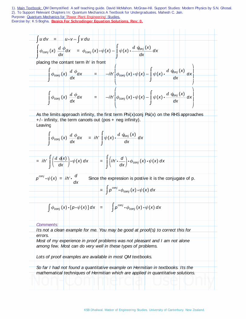
1). Main Textbook: QM Demystified: A self teaching guide. David McMahon. McGraw-Hil. Support Studies: Modern Physics by S.N. Ghosal. 2). To Support Relevant Chapters In: Quantum Mechanics A Textbook for Undergraduates. Mahesh C. Jain. Purpose: Quantum Mechanics for 'Power Plant Engineering' Studies. Exercise by: K S Bogha. Basics For Schrodinger Equation Solutions. Rev: 0.
⌠⌡ du v = −⋅u v ⌠⌡ dv u⌠⎮⌡
dϕconj ((x)) ― ―dϕdx
x = −⋅ϕconj ((x)) ψ((x))⌠⎮⌡
d⋅ψ((x)) ― ― ― ―dϕconj ((x))
dxx
placing the contant term ih' in front⌠⎮⌡
dϕconj ((x)) ― ―dϕdx
x = −ih'
⎛⎜⎜⎜⎝
−⋅ϕconj ((x)) ψ((x))⌠⎮⌡
d⋅ψ((x)) ― ― ― ―dϕconj ((x))
dxx
⎞⎟⎟⎟⎠
⌠⎮⌡
dϕconj ((x)) ― ―dϕdx
x = −ih'
⎛⎜⎜⎜⎝
−⋅ϕconj ((x)) ψ((x))⌠⎮⌡
d⋅ψ((x)) ― ― ― ―dϕconj ((x))
dxx
⎞⎟⎟⎟⎠
As the limits approach infinity, the first term Phi(x)conj Psi(x) on the RHS approaches +/- infinity, the term cancels out (pos + neg infinity). Leaving
⌠⎮⌡
dϕconj ((x)) ― ―dϕdx
x = ih'⌠⎮⌡
d⋅ψ((x)) ― ― ― ―dϕconj ((x))
dxx
= ih'⌠⎮⌡
d⋅⎛⎜⎝― ― ―dϕ((x))
dx⎞⎟⎠ψ((x)) x =
⌠⎮⌡
d⋅⋅⎛⎜⎝⋅ih' ―
ddx⎞⎟⎠ϕconj ((x)) ψ((x)) x
⋅pconj ψ((x)) = ⋅ih' ―d
dxSince the expression is postive it is the conjugate of p.
= ⌠⌡ d⋅⋅pconj ϕconj ((x)) ψ((x)) x
⌠⌡ d⋅ϕconj ((x)) ⋅p ψ((x))[[ ]] x = ⌠
⌡ d⋅⋅pconj ϕconj ((x)) ψ((x)) x
Comments:Its not a clean example for me. You may be good at proof(s) to correct this for errors.Most of my experience in proof problems was not pleasant and I am not alone among few. Most can do very well in these types of problems.
Lots of proof examples are available in most QM textbooks.
So far I had not found a quantitative example on Hermitian in textbooks. Its the mathematical techniques of Hermitian which are applied in quantitative solutions.
KSB Dhaliwal. Master of Engineering Studies. University of Canterbury. New Zealand.

1). Main Textbook: QM Demystified: A self teaching guide. David McMahon. McGraw-Hil. Support Studies: Modern Physics by S.N. Ghosal. 2). To Support Relevant Chapters In: Quantum Mechanics A Textbook for Undergraduates. Mahesh C. Jain. Purpose: Quantum Mechanics for 'Power Plant Engineering' Studies. Exercise by: K S Bogha. Basics For Schrodinger Equation Solutions. Rev: 0.
Notes: Fourier Transform for determing space and momentum wavefunction:
The fact that momentum can be expressed as p = h'k allows us to define a momentum space wavefunction that is related to the position space wavefunction, this is achieved thru the Fourier transform.
Similarly for achieving a position wavefunction from a momentum space wavefunction.
Fourier Transform:
≔f ((x)) ⎛⎜⎝― ―
1
‾‾‾2 π
⎞⎟⎠
⌠⌡ d−∞
∞
⋅F ((k)) e ⋅⋅i k x k positive exp.
≔F ((x)) ⎛⎜⎝― ―
1
‾‾‾2 π
⎞⎟⎠
⌠⌡ d−∞
∞
⋅f ((x)) e ⋅⋅−i k x x negative exp.
So how do we determine the momentum and space wavefunctions:
1). Apply Fourier Transform on momentum space function to get the space wavefunction.
ψ((x)) = ⎛⎜⎝― ― ―
1
‾‾‾‾‾‾⋅2 π h'
⎞⎟⎠
⌠⎮⌡ d−∞
∞
⋅ϕ((P)) e― ―⋅⋅i p x
h' p positive exp.
2). Apply Fourier Transform on position space function to get the momentum wavefunction.
ϕ((p)) = ⎛⎜⎝― ― ―
1
‾‾‾‾‾‾⋅2 π h'
⎞⎟⎠
⌠⎮⌡ d−∞
∞
⋅ψ((x)) e― ―⋅⋅−i p x
h' pnegative exp.
KSB Dhaliwal. Master of Engineering Studies. University of Canterbury. New Zealand.

1). Main Textbook: QM Demystified: A self teaching guide. David McMahon. McGraw-Hil. Support Studies: Modern Physics by S.N. Ghosal. 2). To Support Relevant Chapters In: Quantum Mechanics A Textbook for Undergraduates. Mahesh C. Jain. Purpose: Quantum Mechanics for 'Power Plant Engineering' Studies. Exercise by: K S Bogha. Basics For Schrodinger Equation Solutions. Rev: 0.
Example Problem 6.17 Fourier Transform To Find Momentum. D McMahon.
Suppose that≔ψ((x)) ⎛⎜⎝― ―
1
‾‾a
⎞⎟⎠
-a <= x <= a
Find the momentum space ?Φ((p))Solution:
ϕ((p)) = ⎛⎜⎝― ― ―
1
‾‾‾‾‾‾⋅2 π h'
⎞⎟⎠
⌠⎮⌡ d−∞
∞
⋅ψ((x)) e― ―⋅⋅−i p x
h' p
= ⎛⎜⎝― ― ―
1
‾‾‾‾‾‾⋅2 π h'
⎞⎟⎠
⌠⎮⎮⌡
d
−∞
∞
⋅⎛⎜⎝― ―
1
‾‾a
⎞⎟⎠
e― ―⋅⋅−i p x
h' p
= ⎛⎜⎝― ― ―
1
‾‾‾‾‾‾⋅2 π h'
⎞⎟⎠
⎛⎜⎝― ―
1
‾‾a
⎞⎟⎠
⎛⎜⎝― ―
h'⋅−i p⎞⎟⎠
⎛⎜⎝e― ―⋅⋅−i p x
h'⎞⎟⎠
lim a to -a
Set the exponential term to a form that can be replaced by asimplied trig term
= ⎛⎜⎝― ― ―
1
‾‾‾‾‾‾⋅2 π h'
⎞⎟⎠
⎛⎜⎝― ―
1
‾‾a
⎞⎟⎠
⎛⎜⎝― ―2 h'
p⎞⎟⎠
⎛⎜⎜⎝― ― ― ― ―
−e― ―⋅⋅i p x
h' e― ―⋅⋅−i p x
h'
2i
⎞⎟⎟⎠
= ⎛⎜⎝― ― ―
2 h'
‾‾‾2 h'
⎞⎟⎠
⎛⎜⎝― ―
1
‾‾π
⎞⎟⎠
⎛⎜⎝― ―
1
‾‾a
⎞⎟⎠
⎛⎜⎝―1p⎞⎟⎠
⎛⎜⎜⎝― ― ― ― ―
−e― ―⋅⋅i p a
h' e― ―⋅⋅−i p a
h'
2i
⎞⎟⎟⎠
=⎛⎜⎝― ― ―‾‾‾2 h'1
⎞⎟⎠⎛⎜⎝― ―
1
‾‾π
⎞⎟⎠
⎛⎜⎝― ―
1
‾‾a
⎞⎟⎠
⎛⎜⎝―1p⎞⎟⎠
⎛⎜⎜⎝― ― ― ― ―
−e― ―⋅⋅i p a
h' e― ―⋅⋅−i p a
h'
2i
⎞⎟⎟⎠
= ⋅⋅⎛⎜⎝―aa⎞⎟⎠⎛⎜⎝―h'h'⎞⎟⎠
⎛⎜⎜⎝― ― ―‾‾‾2 h'
‾‾‾πa
⎞⎟⎟⎠
⎛⎜⎝―1p⎞⎟⎠
sin⎛⎜⎝―pah'⎞⎟⎠
= ⋅⎛⎜⎝―ah'⎞⎟⎠
⎛⎜⎜⎝― ― ―‾‾‾2 h'
‾‾‾πa
⎞⎟⎟⎠
⎛⎜⎝―h'pa⎞⎟⎠
sin⎛⎜⎝―pah'⎞⎟⎠
= ⋅⎛⎜⎜⎝― ―‾‾a
‾‾h'
⎞⎟⎟⎠
⎛⎜⎜⎝― ―‾‾2
‾‾π
⎞⎟⎟⎠
⎛⎜⎝―h'pa⎞⎟⎠
sin⎛⎜⎝―pah'⎞⎟⎠
= ⋅⎛⎜⎜⎝― ―‾‾‾2 a
‾‾‾πh'
⎞⎟⎟⎠
⎛⎜⎝―h'pa⎞⎟⎠
sin⎛⎜⎝―pah'⎞⎟⎠
= ⋅⎛⎜⎜⎝― ―‾‾‾2 a
‾‾‾πh'
⎞⎟⎟⎠― ― ―sin⎛⎜⎝―pah'⎞⎟⎠
⎛⎜⎝―pah'⎞⎟⎠
= ⋅⎛⎜⎜⎝― ―‾‾‾2 a
‾‾‾πh'
⎞⎟⎟⎠
sinc⎛⎜⎝―pah'⎞⎟⎠
Ans.
KSB Dhaliwal. Master of Engineering Studies. University of Canterbury. New Zealand.

1). Main Textbook: QM Demystified: A self teaching guide. David McMahon. McGraw-Hil. Support Studies: Modern Physics by S.N. Ghosal. 2). To Support Relevant Chapters In: Quantum Mechanics A Textbook for Undergraduates. Mahesh C. Jain. Purpose: Quantum Mechanics for 'Power Plant Engineering' Studies. Exercise by: K S Bogha. Basics For Schrodinger Equation Solutions. Rev: 0.
Example Problem 6.18 Fourier Transform To Find Position. D McMahon.
Suppose that
≔ϕ((k)) e⋅⎛⎝−―
ab⎞⎠(( −k k0))
2
Use the fourier Transform to find ψ((p))
Solution:
ψ((x)) = ⎛⎜⎝― ―
1
‾‾‾2 π
⎞⎟⎠
⌠⌡ d−∞
∞
⋅ψ((k)) e ⋅⋅i k x k
= ⎛⎜⎝― ―
1
‾‾‾2 π
⎞⎟⎠
⌠⎮⌡ d−∞
∞
⋅⎛⎜⎝e
⋅⎛⎝−―ab⎞⎠(( −k k0))
2⎞⎟⎠e ⋅⋅i k x k
The 2 exponential terms makes it difficult to intergrate. Here attempting to manually do this is not an option. So we will use intergral tables. The form provided below.
⌠⎮⌡ d−∞
∞
⋅e−αu2
eβu u = ⋅‾‾―πa
e―β
2
4α
Let u = ⋅⎛⎝−k k0⎞⎠‾‾―ab
≔dk ⎛⎝−k k0⎞⎠ u = ⋅dk‾‾―ab
⎛⎜⎝‾‾―ba
⎞⎟⎠
u = ⎛⎝−k k0⎞⎠
k = +⎛⎜⎝‾‾―ba
⎞⎟⎠
u k0
Substitute the terms above into the intergral expression.
= ⎛⎜⎝― ―
1
‾‾‾2 π
⎞⎟⎠
⌠⎮⌡ d−∞
∞
⋅⎛⎜⎝e
⋅⎛⎝−―ab⎞⎠(( −k k0))
2⎞⎟⎠e ⋅⋅i k x k = ⋅⎛
⎜⎝― ―
1
‾‾‾2 π
⎞⎟⎠
⎛⎜⎝‾‾―ba
⎞⎟⎠
⌠⎮⌡ d−∞
∞
⋅⎛⎝eu
2⎞⎠e
⋅⋅i ⎛⎝ +⎛⎝‾‾―ba⎞⎠u k0
⎞⎠x
u
⋅⋅⎛⎜⎝― ―
1
‾‾‾2 π
⎞⎟⎠
⎛⎜⎝‾‾―ba
⎞⎟⎠
e ik0x⌠⎮⌡ d−∞
∞
⋅⎛⎝eu
2⎞⎠e
⋅⋅i ⎛⎝‾‾―ba⎞⎠u x
u <---rearranging
Lets match up the table integral form to the expression above.
⌠⎮⌡ d−∞
∞
⋅e−αu2
eβu u
From⎛⎝eu
2⎞⎠ ≔α 1 From e
⋅⋅i ⎛⎝‾‾―ba⎞⎠u x
≔β ⋅⋅i⎛⎜⎝‾‾―ba
⎞⎟⎠
x
KSB Dhaliwal. Master of Engineering Studies. University of Canterbury. New Zealand.

1). Main Textbook: QM Demystified: A self teaching guide. David McMahon. McGraw-Hil. Support Studies: Modern Physics by S.N. Ghosal. 2). To Support Relevant Chapters In: Quantum Mechanics A Textbook for Undergraduates. Mahesh C. Jain. Purpose: Quantum Mechanics for 'Power Plant Engineering' Studies. Exercise by: K S Bogha. Basics For Schrodinger Equation Solutions. Rev: 0.
⋅‾‾―πa
e―β
2
4α <--- The solution form from tables.
Next plug-in the values for alpha and beta: ⋅‾‾―π1
e― ― ― ―⎛⎝ ⋅⋅i ⎛⎝
‾‾―ba⎞⎠x⎞⎠
2
4
=⋅‾‾π e― ― ―
⋅−1⎛⎝―ba⎞⎠x
2
4
=⋅‾‾π e−⎛⎝― ―⋅b x
2
⋅a 4
⎞⎠
Now presenting the full integral with the constant terms:
ψ((x)) = ⋅⋅⋅⎛⎜⎝― ―
1
‾‾‾2 π
⎞⎟⎠
⎛⎜⎝‾‾―ba
⎞⎟⎠
e ik0x
⎛⎜⎝ ⋅‾‾π e
−⎛⎝― ―⋅b x
2
⋅a 4
⎞⎠⎞⎟⎠
ψ((x)) = ⋅⋅⎛⎜⎝‾‾‾‾― ―
b2 a
⎞⎟⎠
e ik0x
⎛⎜⎝e−⎛⎝― ―⋅b x
2
⋅a 4
⎞⎠⎞⎟⎠ Ans. The space wavefunction
KSB Dhaliwal. Master of Engineering Studies. University of Canterbury. New Zealand.

1). Main Textbook: QM Demystified: A self teaching guide. David McMahon. McGraw-Hil. Support Studies: Modern Physics by S.N. Ghosal. 2). To Support Relevant Chapters In: Quantum Mechanics A Textbook for Undergraduates. Mahesh C. Jain. Purpose: Quantum Mechanics for 'Power Plant Engineering' Studies. Exercise by: K S Bogha. Basics For Schrodinger Equation Solutions. Rev: 0.
Example 6.19 Uncertainty Principle. D McMahon.
A particle of mass m in a one dimensional box is found to be in the ground state:
≔ψ((x)) ⋅⎛⎜⎝‾‾―2a
⎞⎟⎠
sin⎛⎜⎝― ―⋅π xa⎞⎟⎠
Find for this state.ΔxΔp
Solution:
One dimensional box we set the upper limit a and lower limit 0.
We know we can define momentum p as: ⋅−ih' ―d
dx
momentum p^2 as: ⋅−ih' ― ―d2
dx2
We need to calculate:
1). ⌠⌡ d0
a
⋅⋅ψconj ((x)) p ψ((x)) x
2). ⌠⌡ d0
a
⋅⋅ψconj ((x)) p2 ψ((x)) x
Then the same for x.Right most 2 terms of 1 and 2 above:
⋅p ψ((x)) = ⋅−ih' ―d
dx‾‾―2a
sin⎛⎜⎝― ―πxa⎞⎟⎠= ⋅⋅−ih'
‾‾―2a⎛⎜⎝―πa⎞⎟⎠
cos⎛⎜⎝― ―πxa⎞⎟⎠
= ⋅−― ―ih'π
a‾‾―2a
cos⎛⎜⎝― ―πxa⎞⎟⎠
⋅p2 ψ((x))= ―ddx
ih'⎛⎜⎝
⋅−― ―ih'π
a‾‾―2a
cos⎛⎜⎝― ―πxa⎞⎟⎠
⎞⎟⎠
= ⋅⋅⎛⎝ ⋅i2 h'2⎞⎠‾‾―2a
⎛⎜⎝― ―π2
a2
⎞⎟⎠−sin⎛⎜⎝
― ―πxa⎞⎟⎠
= ⋅⋅−⎛⎝h'2⎞⎠‾‾―2a
⎛⎜⎝― ―π2
a2
⎞⎟⎠
sin⎛⎜⎝― ―πxa⎞⎟⎠
= ⋅−⎛⎜⎝― ― ―⋅h'2 π2
a2
⎞⎟⎠
‾‾―2a
sin⎛⎜⎝― ―πxa⎞⎟⎠
<p>= ⌠⌡ d0
a
⋅⋅ψconj ((x)) p ψ((x)) x = −⌠⎮⌡
d⋅⋅‾‾―2a
sin⎛⎜⎝― ―πxa⎞⎟⎠― ―ih'π
a‾‾―2a
cos⎛⎜⎝― ―πxa⎞⎟⎠
x
= −⎛⎜⎝― ― ―⋅2 ih'π
a2
⎞⎟⎠
⌠⎮⌡
d⋅sin⎛⎜⎝― ―πxa⎞⎟⎠
cos⎛⎜⎝― ―πxa⎞⎟⎠
x
We did this intergral in a previous example.
KSB Dhaliwal. Master of Engineering Studies. University of Canterbury. New Zealand.

1). Main Textbook: QM Demystified: A self teaching guide. David McMahon. McGraw-Hil. Support Studies: Modern Physics by S.N. Ghosal. 2). To Support Relevant Chapters In: Quantum Mechanics A Textbook for Undergraduates. Mahesh C. Jain. Purpose: Quantum Mechanics for 'Power Plant Engineering' Studies. Exercise by: K S Bogha. Basics For Schrodinger Equation Solutions. Rev: 0.
<p> = −⎛⎜⎝― ― ―⋅2 ih'π
a2
⎞⎟⎠−cos2 ⎛
⎜⎝― ―⋅π xa⎞⎟⎠
⎡⎢⎣
⎤⎥⎦ Lim x = a to 0
a: ⎛⎜⎝― ― ―⋅2 ih'π
a2
⎞⎟⎠
cos2 ((π))⎡⎣ ⎤⎦ = ⎛⎜⎝― ― ―⋅2 ih'π
a2
⎞⎟⎠
cos(pi) = -1, cos^2(pi) = 1
0: ⎛⎜⎝― ― ―⋅2 ih'π
a2
⎞⎟⎠
cos2 ((0))⎡⎣ ⎤⎦ = ⎛⎜⎝― ― ―⋅2 ih'π
a2
⎞⎟⎠
cos(0) = 1, cos^2(0) = 1
Result limit a to 0:
<p> = −⎛⎜⎝― ― ―⋅2 ih'π
a2
⎞⎟⎠
⎛⎜⎝― ― ―⋅2 ih'π
a2
⎞⎟⎠
= 0
<p^2> = ⌠⌡ d0
a
⋅⋅ψconj ((x)) p2 ψ((x)) x
⌠⎮⎮⌡
d
0
a
⋅⎛⎜⎝
⋅−⎛⎜⎝‾‾―2a
⎞⎟⎠
sin⎛⎜⎝― ―⋅π xa⎞⎟⎠
⎞⎟⎠
⎛⎜⎝
⋅−⎛⎜⎝― ― ―⋅h'2 π2
a2
⎞⎟⎠
‾‾―2a
sin⎛⎜⎝― ―πxa⎞⎟⎠
⎞⎟⎠
x
⌠⎮⎮⌡
d
0
a
⋅⎛⎜⎝
⋅⎛⎜⎝‾‾―2a
⎞⎟⎠
sin⎛⎜⎝― ―⋅π xa⎞⎟⎠
⎞⎟⎠
⎛⎜⎝
⋅⎛⎜⎝― ― ―⋅h'2 π2
a2
⎞⎟⎠
‾‾―2a
sin⎛⎜⎝― ―πxa⎞⎟⎠
⎞⎟⎠
x
⋅⋅⎛⎜⎝―2a⎞⎟⎠
⎛⎜⎝― ― ―⋅h'2 π2
a2
⎞⎟⎠
⌠⎮⌡
d
0
a
⎛⎜⎝
⋅sin2 ⎛⎜⎝― ―⋅π xa⎞⎟⎠⎞⎟⎠
x
⋅⎛⎜⎝― ― ― ―
⋅⋅2 h'2 π2
a3
⎞⎟⎠
⌠⎮⌡
d
0
a
⎛⎜⎝
⋅sin2 ⎛⎜⎝― ―⋅π xa⎞⎟⎠⎞⎟⎠
x
⋅⎛⎜⎝―12⎞⎟⎠
⌠⎮⌡
d
0
a
−1 ⎛⎜⎝⋅cos ⎛⎜⎝― ― ―
⋅⋅2 π xa⎞⎟⎠⎞⎟⎠
x = ⎛⎜⎝―12⎞⎟⎠⎛⎜⎝−x ⋅⎛⎜⎝― ―2 π
a⎞⎟⎠
sin⎛⎜⎝― ― ―
⋅⋅2 π xa⎞⎟⎠⎞⎟⎠
= ⎛⎜⎝−―
x2
⋅⎛⎜⎝―πa⎞⎟⎠
sin⎛⎜⎝― ― ―
⋅⋅2 π xa⎞⎟⎠⎞⎟⎠
Lim a to 0 = −⎛⎜⎝―a2⎞⎟⎠
0 = ⎛⎜⎝―a2⎞⎟⎠
<p^2> = ⋅⎛⎜⎝― ― ― ―
⋅⋅2 h'2 π2
a3
⎞⎟⎠
⎛⎜⎝―a2⎞⎟⎠
=⎛⎜⎝― ― ―⋅h'2 π2
a2
⎞⎟⎠
KSB Dhaliwal. Master of Engineering Studies. University of Canterbury. New Zealand.

1). Main Textbook: QM Demystified: A self teaching guide. David McMahon. McGraw-Hil. Support Studies: Modern Physics by S.N. Ghosal. 2). To Support Relevant Chapters In: Quantum Mechanics A Textbook for Undergraduates. Mahesh C. Jain. Purpose: Quantum Mechanics for 'Power Plant Engineering' Studies. Exercise by: K S Bogha. Basics For Schrodinger Equation Solutions. Rev: 0.
Δp = ‾‾‾‾‾‾‾‾‾−⎛⎝p2⎞⎠ ((p))2
=‾‾‾‾‾‾‾‾‾‾
−⎛⎜⎝― ― ―⋅h'2 π2
a2
⎞⎟⎠
0
Δp = ― ―⋅h' πa
Solved for delta p.
Next solve for delta x:<x> : ⌠
⌡ d0
a
⋅⋅ψconj ((x)) x ψ((x)) x
and
<x^2> : ⌠⌡ d0
a
⋅⋅ψconj ((x)) x2 ψ((x)) x
<x> :⌠⎮⌡
d
0
a
⋅⎛⎜⎝‾‾―2a
⎞⎟⎠
sin⎛⎜⎝― ―⋅π xa⎞⎟⎠
((x))⎛⎜⎝‾‾―2a
⎞⎟⎠
sin⎛⎜⎝― ―⋅π xa⎞⎟⎠
x
= ⋅⎛⎜⎝―2a⎞⎟⎠
⌠⎮⌡
d
0
a
⋅⋅x sin2 ⎛⎜⎝― ―⋅π xa⎞⎟⎠
x See example 6.9 for the steps.
<x> : ―a2
<x^2> : ⌠⌡ d0
a
⋅⋅ψconj ((x)) x2 ψ((x)) x
= ⋅⎛⎜⎝―2a⎞⎟⎠
⌠⎮⌡
d
0
a
⋅⋅x2 sin2 ⎛⎜⎝― ―⋅π xa⎞⎟⎠
x Follow example 6.9 change x for x^2
= ⋅⎛⎜⎝―2a⎞⎟⎠⌠⌡ d0
a
x2 x - ⋅⎛⎜⎝―1a⎞⎟⎠
⌠⎮⌡
d
0
a
⋅x2 ⎛⎜⎝cos⎛⎜⎝― ― ―
⋅⋅2 π xa⎞⎟⎠⎞⎟⎠
x
First term:
⋅⋅⎛⎜⎝―2a⎞⎟⎠⎛⎜⎝―13⎞⎟⎠
x3 = ⋅⋅⎛⎜⎝―2a⎞⎟⎠⎛⎜⎝―13⎞⎟⎠
a3 = ⋅⎛⎜⎝―23⎞⎟⎠
a2
Lim a - 0
KSB Dhaliwal. Master of Engineering Studies. University of Canterbury. New Zealand.

1). Main Textbook: QM Demystified: A self teaching guide. David McMahon. McGraw-Hil. Support Studies: Modern Physics by S.N. Ghosal. 2). To Support Relevant Chapters In: Quantum Mechanics A Textbook for Undergraduates. Mahesh C. Jain. Purpose: Quantum Mechanics for 'Power Plant Engineering' Studies. Exercise by: K S Bogha. Basics For Schrodinger Equation Solutions. Rev: 0.
Second term apply intergration by parts.
⋅⎛⎜⎝―1a⎞⎟⎠
⌠⎮⌡
d
0
a
⋅x2 ⎛⎜⎝cos⎛⎜⎝― ― ―
⋅⋅2 π xa⎞⎟⎠⎞⎟⎠
x
Let ―dydx
= ⋅x2 ⎛⎜⎝cos⎛⎜⎝― ― ―⋅2 π x
a⎞⎟⎠⎞⎟⎠
dy = ⋅x2 cos⎛⎜⎝― ― ―⋅2 π x
a⎞⎟⎠
dx
Let u = x2― ―dudx
= 2 x
so du = ⋅2 x dx
―dvdx
= ⎛⎜⎝cos⎛⎜⎝― ― ―⋅2 π x
a⎞⎟⎠⎞⎟⎠
dv = ⎛⎜⎝cos⎛⎜⎝― ― ―⋅2 π x
a⎞⎟⎠⎞⎟⎠
dx
⌠⌡ d1 v =⌠⎮⌡
d⎛⎜⎝cos⎛⎜⎝― ― ―⋅2 π x
a⎞⎟⎠⎞⎟⎠
x
v = ⋅⎛⎜⎝― ―
a⋅2 π⎞⎟⎠⎛⎜⎝sin⎛⎜⎝― ― ―⋅2 π x
a⎞⎟⎠⎞⎟⎠
⌠⌡ du v = −⋅u v ⌠⌡ dv u
⌠⌡ du v =⌠⎮⌡
d⋅x2 ⎛⎜⎝cos⎛⎜⎝
― ― ―⋅2 π x
a⎞⎟⎠⎞⎟⎠
x
⋅u v = ⋅⎛⎜⎝― ―⋅a x2
⋅2 π
⎞⎟⎠⎛⎜⎝sin⎛⎜⎝― ― ―⋅2 π x
a⎞⎟⎠⎞⎟⎠
⌠⌡ dv u =⌠⎮⌡
d⋅⋅⎛⎜⎝― ―
a⋅2 π⎞⎟⎠⎛⎜⎝sin⎛⎜⎝― ― ―⋅2 π x
a⎞⎟⎠⎞⎟⎠
2 x x
=⌠⎮⌡
d⋅⎛⎜⎝― ―⋅a xπ⎞⎟⎠⎛⎜⎝sin⎛⎜⎝― ― ―⋅2 π x
a⎞⎟⎠⎞⎟⎠
x
KSB Dhaliwal. Master of Engineering Studies. University of Canterbury. New Zealand.

1). Main Textbook: QM Demystified: A self teaching guide. David McMahon. McGraw-Hil. Support Studies: Modern Physics by S.N. Ghosal. 2). To Support Relevant Chapters In: Quantum Mechanics A Textbook for Undergraduates. Mahesh C. Jain. Purpose: Quantum Mechanics for 'Power Plant Engineering' Studies. Exercise by: K S Bogha. Basics For Schrodinger Equation Solutions. Rev: 0.
Placing the terms in order:
⌠⌡ du v = −⋅u v ⌠⌡ dv u⌠⎮⌡
d⋅x2 ⎛⎜⎝cos⎛⎜⎝― ― ―⋅2 π x
a⎞⎟⎠⎞⎟⎠
x = ⋅⎛⎜⎝― ―ax2
⋅2 π
⎞⎟⎠⎛⎜⎝sin⎛⎜⎝― ― ―⋅2 π x
a⎞⎟⎠⎞⎟⎠
-⌠⎮⌡
d⋅⎛⎜⎝― ―⋅a xπ⎞⎟⎠⎛⎜⎝sin⎛⎜⎝― ― ―⋅2 π x
a⎞⎟⎠⎞⎟⎠
x
= +⋅⎛⎜⎝― ―ax2
⋅2 π
⎞⎟⎠⎛⎜⎝sin⎛⎜⎝― ― ―⋅2 π x
a⎞⎟⎠⎞⎟⎠
⋅⎛⎜⎝― ―⋅a xπ⎞⎟⎠⎛⎜⎝― ―
a2 π⎞⎟⎠⎛⎜⎝cos⎛⎜⎝― ― ―⋅2 π x
a⎞⎟⎠⎞⎟⎠
= +⋅⎛⎜⎝― ―ax2
⋅2 π
⎞⎟⎠
sin⎛⎜⎝― ― ―⋅2 π x
a⎞⎟⎠
⋅⎛⎜⎝― ―a2 x
2 π2
⎞⎟⎠
cos⎛⎜⎝― ― ―⋅2 π x
a⎞⎟⎠
Taking the limit a - 0Lim a:
= +⋅⎛⎜⎝― ―
a3
⋅2 π
⎞⎟⎠
sin ((2 π)) ⋅⎛⎜⎝― ―
a3
2 π2
⎞⎟⎠
cos ((2 π)) =⎛⎜⎝― ―
a3
2 π2
⎞⎟⎠
Note: =cos ((2 π)) 1sin ((2 π))= 1
Lim 0:= 0
⋅⎛⎜⎝―1a⎞⎟⎠
⌠⎮⌡
d
0
a
⋅x2 ⎛⎜⎝cos⎛⎜⎝― ― ―
⋅⋅2 π xa⎞⎟⎠⎞⎟⎠
x = ⋅⎛⎜⎝―1a⎞⎟⎠
⎛⎜⎝― ―
a3
2 π2
⎞⎟⎠= ― ―a2
2 π2The 2nd term's result.
Final result for the integral ⋅⎛⎜⎝―2a⎞⎟⎠⌠⌡ d0
a
x2 x - ⋅⎛⎜⎝―1a⎞⎟⎠
⌠⎮⌡
d
0
a
⋅x2 ⎛⎜⎝cos⎛⎜⎝― ― ―
⋅⋅2 π xa⎞⎟⎠⎞⎟⎠
x
= −⎛⎜⎝― ―2 a2
3
⎞⎟⎠
⎛⎜⎝― ―
a2
2 π2
⎞⎟⎠
< > x2 = ⋅⎛⎜⎝―a2
6
⎞⎟⎠⎛⎜⎝−2 ― ―
3
π2
⎞⎟⎠
Δx = ‾‾‾‾‾‾‾‾‾−⎛⎝x2⎞⎠ ((x))2
=‾‾‾‾‾‾‾‾‾‾‾‾‾‾‾‾‾‾‾
−⎛⎜⎝
⋅⎛⎜⎝―a2
6
⎞⎟⎠⎛⎜⎝−2 ― ―
3
π2
⎞⎟⎠
⎞⎟⎠
⎛⎜⎝―a2⎞⎟⎠
2
OR‾‾‾‾‾‾‾‾‾‾‾‾‾‾‾‾‾‾
−−⎛⎜⎝― ―2 a2
3
⎞⎟⎠
⎛⎜⎝― ―
a2
2 π2
⎞⎟⎠
⎛⎜⎝―a2⎞⎟⎠
2
=‾‾‾‾‾‾‾‾‾‾‾‾‾‾‾‾‾‾
−−⎛⎜⎝― ―2 a2
3
⎞⎟⎠
⎛⎜⎝― ―
a2
2 π2
⎞⎟⎠
⎛⎜⎝―a2
4
⎞⎟⎠
= a‾‾‾‾‾‾‾‾‾‾‾‾‾‾‾
−−⎛⎜⎝―23⎞⎟⎠⎛⎜⎝― ―
1
2 π2
⎞⎟⎠
⎛⎜⎝―14⎞⎟⎠
= a‾‾‾‾‾‾‾‾‾‾‾‾‾
−⎛⎜⎝― ―−8 312⎞⎟⎠⎛⎜⎝― ―
1
2 π2
⎞⎟⎠
= ―aπ
‾‾‾‾‾‾‾‾‾‾‾−
⎛⎜⎝― ―5 π2
12
⎞⎟⎠⎛⎜⎝―6
12⎞⎟⎠
Δx = ―aπ
‾‾‾‾‾‾‾― ― ―
−5 π2 612
= ⋅0.605 a
KSB Dhaliwal. Master of Engineering Studies. University of Canterbury. New Zealand.

1). Main Textbook: QM Demystified: A self teaching guide. David McMahon. McGraw-Hil. Support Studies: Modern Physics by S.N. Ghosal. 2). To Support Relevant Chapters In: Quantum Mechanics A Textbook for Undergraduates. Mahesh C. Jain. Purpose: Quantum Mechanics for 'Power Plant Engineering' Studies. Exercise by: K S Bogha. Basics For Schrodinger Equation Solutions. Rev: 0.
Now we solve for: ΔxΔp= (( ⋅0.605 a)) ⎛⎜⎝― ―⋅h' πa⎞⎟⎠
= ((0.605 π)) ((h'))
ΔxΔp= ((1.901)) ((h'))is greater than h'. Ans.
Uncertainty relation Chapter 9 section 13 (9.13) in Atomic Physics (SN Ghoshal):
≥ΔxΔph'
Section 10.13 Formal proof of the Uncertainty Relation (SN Ghoshal): >ΔxΔp―
h'2
The Hisenberg uncertainty principle : ≥ΔxΔph' page 56 QM Demystified D McMahon.
Page 232 Atomic Physics (SN Ghoshal):Thus the wave representation of the particle implies some uncertainty delta-x of the position x of the particle and a corresponding uncertainty delta-p in specifying itsmomentum p simultneously.
The more exactly we want to localise the particle (smaller uncertainty delta-x in the position x) the less exactly specified will be the momentum (greater uncertainty delta-p in the momentum p). Heisenberg was the first to point out this inherent limitation in specifying the position and momentum of a particle regarded as a wave, which is known as the uncertainty principle.
Comments:
Some relief is here because D McMahon wrote the book QM Demystified.
There is the Schaum's Series books they have a QM book. If you have seen or used Schaum's Series books, they are helpful. In this case for QM McMahon's book is effective on the subject material for what he is delivering at UG level.
We have not touched on Schrodinger's Equation for what it can do in QM, just a some mathmatics on how to apply Schrodinger's Equation.
This is just at the introduction level, knowing advanced mathematics there maybe untold math to encounter. To that level I am not prepared to engage, maybe most of you are the same here on that. Most NOT all!
KSB Dhaliwal. Master of Engineering Studies. University of Canterbury. New Zealand.

1). Main Textbook: QM Demystified: A self teaching guide. David McMahon. McGraw-Hil. Support Studies: Modern Physics by S.N. Ghosal. 2). To Support Relevant Chapters In: Quantum Mechanics A Textbook for Undergraduates. Mahesh C. Jain. Purpose: Quantum Mechanics for 'Power Plant Engineering' Studies. Exercise by: K S Bogha. Basics For Schrodinger Equation Solutions. Rev: 0.
Notes on Probability Current Density.
Electromagnetic theory has something similar, current density, if not first encountered in that subject matter. Not exactly the same here. Electromagnetic theory has it's famous Maxwell's equation.If you remember how Green's theorem or Gauss' divergence theorem from calculus which was applied in electromagnetic theory. Here is not a form of QM with special value to electrical engineering. So, take that thought out again its QM.The understanding on probability current density can be achieved from all modern physics or QM textbooks.
Some key equations are presented here you look up their explanations wrt QM.From QM For UG (Mahesh Jain) pages 101 - 102:
How to read the equations below above: If a particle is descriibed by a wavefunction PSI(r,t), then the probability of finding the particle, at time t, within the volume element dr = dxdydz about the point r = (x,y,z) is:
P (( ,r t)) dr = ||Ψ(( ,r t))||2
dr = Ψconj ((r.t)) Ψ(( ,r t)) dr
P (( ,r t)) = ||Ψ(( ,r t))||2
= Ψconj ((r.t)) Ψ(( ,r t)) <-- Position probability density.⌠⎮⌡ d||Ψ(( ,r t))||
2r = 1 Since probability of finding the particle somewhere at time t is unity,
the wavefunction is chosen to satisfy the normilisation condition.
Short exercise here to form an equation:
= ++― ―d
d
2
x2― ―d
d
2
y2― ―d
d
2
z2
Becaue of the text editor limitation on the version here, another symbol is used:
Δ''2 = = ++― ―d
d
2
x2― ―d
d
2
y2― ―d
d
2
z2
ih'⎛⎜⎝― ―dΨdt⎞⎟⎠
= +⎛⎜⎝−― ―
h'2
2 m
⎞⎟⎠Δ''2 Ψ VΨ <---1st expression
and
−ih'⎛⎜⎝― ― ―dΨconj
dt
⎞⎟⎠
= +⎛⎜⎝−― ―
h'2
2 m
⎞⎟⎠Δ''2 Ψconj VΨconj<---2nd expression,
complex conjugate of 1st term
Where V (( ,r t)) in both the 1st and 2nd expression is assumed to be real.V being the potential difference should be real.
KSB Dhaliwal. Master of Engineering Studies. University of Canterbury. New Zealand.

1). Main Textbook: QM Demystified: A self teaching guide. David McMahon. McGraw-Hil. Support Studies: Modern Physics by S.N. Ghosal. 2). To Support Relevant Chapters In: Quantum Mechanics A Textbook for Undergraduates. Mahesh C. Jain. Purpose: Quantum Mechanics for 'Power Plant Engineering' Studies. Exercise by: K S Bogha. Basics For Schrodinger Equation Solutions. Rev: 0.
We want to show:― ―d
dt⌠⌡ dP (( ,r t)) r = ― ―
d
dt
⌠⌡ dΨconj ((r.t)) Ψ(( ,r t)) r = 0
Taking derivative on the LHS wrt time, saying lets see what happens when time changes. Multiply the LHS of 1st term by Ψconj
ih'⎛⎜⎝Ψconj
― ―dΨdt⎞⎟⎠
= +⋅⎛⎜⎝−― ―
h'2
2 m
⎞⎟⎠Ψconj Δ''2 Ψ ⋅Ψconj VΨ <--- 3 rd expression
Multiply the LHS of 2nd expression byΨ
−ih'⎛⎜⎝Ψ― ― ―dΨconj
dt
⎞⎟⎠
= +⋅⎛⎜⎝−― ―
h'2
2 m
⎞⎟⎠Ψ Δ''2 Ψconj ⋅Ψ VΨconj <--- 4 th expression
Subtract expression 4 from 3; 3 -4:
ih'⎛⎜⎝+Ψconj
― ―dΨdt
⋅Ψ ― ―dΨdt⎞⎟⎠
= −⋅⎛⎜⎝−― ―
h'2
2 m
⎞⎟⎠Ψconj Δ''2 Ψ ⋅
⎛⎜⎝−― ―
h'2
2 m
⎞⎟⎠Ψ Δ''2 Ψconj <--- 5th
expression
ih'⎛⎜⎝+Ψconj
― ―dΨdt
⋅Ψ ― ―dΨdt⎞⎟⎠
= ⋅⎛⎜⎝−― ―
h'2
2 m
⎞⎟⎠⎛⎝ −⋅Ψconj Δ''2 Ψ ⋅Ψ Δ''2 Ψconj⎞⎠
Note: =−―1i
1i
⎛⎜⎝
+Ψconj― ―dΨdt
⋅Ψ ― ―dΨdt⎞⎟⎠
= ⋅⎛⎜⎝― ―
ih'2 m⎞⎟⎠⎛⎝ −⋅Ψconj Δ''2 Ψ ⋅Ψ Δ''2 Ψconj⎞⎠
⎛⎜⎝
+Ψconj― ―dΨdt
⋅Ψ ― ―dΨdt⎞⎟⎠
<--- This term on the LHS is the derivative of the product PSI_conj(x) and PSI(x).
Consider the time derivative of the intergral, term above, over a finite volume V:
― ―d
dt
⌠⌡ dV
⎛⎝ ⋅Ψconj Ψ⎞⎠ r = ― ―d
dt
⌠⎮⌡
d
V
⎛⎜⎝
+Ψconj― ―dΨdt
⋅Ψ ― ―dΨdt⎞⎟⎠
r
= ⋅⎛⎜⎝― ―
ih'2 m
⎞⎟⎠⌠⌡ dV
⎛⎝ −⋅Ψconj Δ''2 Ψ ⋅Ψ Δ''2 Ψconj⎞⎠ r
= ⋅⎛⎜⎝― ―
ih'2 m
⎞⎟⎠⌠⌡ dV
⋅Δ'' ⎛⎝ −⋅Ψconj Δ''Ψ ⋅Ψ Δ''Ψconj⎞⎠ r
We pull out the expression = ⋅⎛⎜⎝― ―
ih'2 m⎞⎟⎠⎛⎝ −⋅Ψconj Δ''Ψ ⋅Ψ Δ''Ψconj⎞⎠ for a vector set it = j(r,t)
j (( ,r t)) = ⋅⎛⎜⎝― ―
ih'2 m
⎞⎟⎠⎛⎝ −⋅Ψconj Δ''Ψ ⋅Ψ Δ''Ψconj⎞⎠ <---vector <--- 6th expression
KSB Dhaliwal. Master of Engineering Studies. University of Canterbury. New Zealand.

1). Main Textbook: QM Demystified: A self teaching guide. David McMahon. McGraw-Hil. Support Studies: Modern Physics by S.N. Ghosal. 2). To Support Relevant Chapters In: Quantum Mechanics A Textbook for Undergraduates. Mahesh C. Jain. Purpose: Quantum Mechanics for 'Power Plant Engineering' Studies. Exercise by: K S Bogha. Basics For Schrodinger Equation Solutions. Rev: 0.
<-- this is the probability current density with proper symbol (copy paste).
j (( ,r t)) = ⋅⎛⎜⎝― ―
ih'2 m
⎞⎟⎠
⎛⎜⎝
−⋅Ψconj― ―d
dt((Ψ)) ⋅Ψ ― ―
d
dt⎛⎝Ψconj⎞⎠
⎞⎟⎠
Extending out by removing the symbol, this is what it is.
j (( ,r t)) = ⋅⎛⎜⎝― ―
ih'2 m
⎞⎟⎠⎛⎝ −⋅Ψconj Δ''Ψ ⋅Ψ Δ''Ψconj⎞⎠ <---repeated her to invert i
Note: =―1i−1i
j (( ,r t)) = ⋅−⎛⎜⎝― ― ―
h'⋅2 i m⎞⎟⎠⎛⎝ −⋅Ψconj Δ''Ψ ⋅Ψ Δ''Ψconj⎞⎠ To get the negative sign in the RHS for
the j term below.
LHS of expression 6 is equal to: ― ―d
dt
⌠⌡ dV
⎛⎝ ⋅Ψconj Ψ⎞⎠ r = ― ―d
dt⌠⌡ dP (( ,r t)) r
Next substitute vector j into the 6th expression:
― ―d
dt⌠⌡ dV
P (( ,r t)) r = −⌠⌡ dV
⋅Δ'' j (( ,r t)) r <---- 7th expression
Using Green's theorem (also called Gauss divergence theorem) we can convert the volume integral on the right into an integral over the surface area S bounding the volume V:
― ―d
dt⌠⌡ dV
P (( ,r t)) r = −⌠⌡ dS
j (( ,r t)) S <----8th term
where the vector dS has magnitude equal to an element dS of the surface Sand is directed along the outward normal to dS.When V is the entire space, as is the case in the normalisation integral, the surface S, in the 8th term, recedes to infinity. Since, a square integrable wave function vanishes at large distances, the surface integral becomes zero and hence the expression below is proved.
― ―d
dt⌠⌡ dP (( ,r t)) r = ― ―
d
dt
⌠⌡ dΨconj ((r.t)) Ψ(( ,r t)) r = 0
How do we read or intepret term 8 above, shown below again?
― ―d
dt⌠⌡ dV
P (( ,r t)) r = −⌠⌡ dS
j (( ,r t)) S <---- 8th term
It says that the rate of change of the probability of finding the particle in a volume Vis equal to the probability flux passing through the surface S bounding V.
It is reasonable therefore to interpret the vector j(r,t) as probability current density OR simply probability current.
j (( ,r t)) <---- probability current.
KSB Dhaliwal. Master of Engineering Studies. University of Canterbury. New Zealand.

1). Main Textbook: QM Demystified: A self teaching guide. David McMahon. McGraw-Hil. Support Studies: Modern Physics by S.N. Ghosal. 2). To Support Relevant Chapters In: Quantum Mechanics A Textbook for Undergraduates. Mahesh C. Jain. Purpose: Quantum Mechanics for 'Power Plant Engineering' Studies. Exercise by: K S Bogha. Basics For Schrodinger Equation Solutions. Rev: 0.
― ―d
dtP (( ,r t)) = −⎛⎝ ⋅Δ'' j (( ,r t))⎞⎠<----7th expression without integral
Rearranging 7th expression:
+― ―d
dtP (( ,r t)) ⋅Δ'' j (( ,r t)) = 0 <----9th expression
The equation/expression above has the familiar form associated with the conservation of matter in a fluid of density P and current density j,in a medium in which there are no sources and sinks. This is called the equation of continuity.
Expression 9 shown with theproper symbol using MS Paint.
Probability current density, expression number 6 shown below, may also be writen as:
j (( ,r t)) = ⋅⎛⎜⎝― ―
ih'2 m
⎞⎟⎠⎛⎝ −⋅Ψconj Δ''Ψ ⋅Ψ Δ''Ψconj⎞⎠
j (( ,r t)) = ⋅Re Ψconj ⎛⎜⎝― ―h'
im⎞⎟⎠Δ''Ψ⎡
⎢⎣⎤⎥⎦
--->
This was how QM A Textbook for UG presented the material, here briefly shown.The same material was presently using different expression in QM Demystified.Your textbook may have one of these two methods, or may be another. When it comes to math I only remember whats shown to me in the textbook presentation it may require I refresh or glance thru some tables, so there maybe several ways to present an equation. Usually the simplest of them is used. Maybe the KISS principle, Keep It Simple Silly.Sometimes it can be hard.
KSB Dhaliwal. Master of Engineering Studies. University of Canterbury. New Zealand.

1). Main Textbook: QM Demystified: A self teaching guide. David McMahon. McGraw-Hil. Support Studies: Modern Physics by S.N. Ghosal. 2). To Support Relevant Chapters In: Quantum Mechanics A Textbook for Undergraduates. Mahesh C. Jain. Purpose: Quantum Mechanics for 'Power Plant Engineering' Studies. Exercise by: K S Bogha. Basics For Schrodinger Equation Solutions. Rev: 0.
Problem 6.20
Calculate the probability current density j(x) for the wave function:
≔ψ((x)) sin (( ⋅3 π x)) e2 x
Solution:
j ((x)) = ⋅⎛⎜⎝― ―
ih'2 m⎞⎟⎠⎛⎝ −⋅Ψconj Δ''Ψ ⋅Ψ Δ''Ψconj⎞⎠
j ((x)) = ⋅⎛⎜⎝― ―
ih'2 m⎞⎟⎠
⎛⎜⎝
−⋅Ψconj― ―
d
dx((Ψ)) ⋅Ψ ― ―
d
dx⎛⎝Ψconj⎞⎠
⎞⎟⎠
this is our probability current density
≔ψ((x)) sin (( ⋅3 π x)) e2i x
≔ψconj ((x)) sin (( ⋅3 π x)) e−2i x
― ―d
dxΨ((x)) = +⋅⋅3 π cos (( ⋅3 π x)) e2i x ⋅((2i)) sin (( ⋅3 π x)) e2i x
― ―d
dxΨconj ((x)) = +⋅⋅3 π cos (( ⋅3 π x)) e−2i x ⋅((2i)) sin (( ⋅3 π x)) e−2i x
Setting up the differentiation expression of the probability current:⎛⎜⎝
−⋅Ψconj― ―
d
dx((Ψ)) ⋅Ψ ― ―
d
dx⎛⎝Ψconj⎞⎠
⎞⎟⎠
= ⎛⎝ ⋅sin (( ⋅3 π x)) e−2i x ⎛⎝ +⋅⋅3 π cos (( ⋅3 π x)) e2i x ⋅2i sin (( ⋅3 π x)) e2i x⎞⎠⎞⎠
- ⎛⎝ ⋅sin (( ⋅3 π x)) e−2i x ⎛⎝ +⋅⋅3 π cos (( ⋅3 π x)) e−2i x ⋅((2i)) sin (( ⋅3 π x)) e−2i x⎞⎠⎞⎠
= +⋅⋅3 π sin (( ⋅3 π x)) cos (( ⋅3 π x)) 2i sin2 (( ⋅3 π x))
- +⋅⋅⋅3 π sin (( ⋅3 π x)) cos (( ⋅3 π x)) e−4 x ⋅((2i)) sin2 (( ⋅3 π x)) e−4 x
= −(( ⋅⋅3 π sin (( ⋅3 π x)) cos (( ⋅3 π x)))) ⎛⎝−1 e−4 x⎞⎠ ⎛⎝2i sin2 (( ⋅3 π x))⎞⎠⎛⎝−1 e−4 x⎞⎠
Improving on the above:
= ⎛⎝−1 e−4 x⎞⎠⎛⎝ −(( ⋅⋅3 π sin (( ⋅3 π x)) cos (( ⋅3 π x)))) ⎛⎝2i sin2 (( ⋅3 π x))⎞⎠⎞⎠
j ((x)) = ⋅⎛⎜⎝― ―
ih'2 m⎞⎟⎠⎛⎝−1 e−4 x⎞⎠⎛⎝ −(( ⋅⋅3 π sin (( ⋅3 π x)) cos (( ⋅3 π x)))) ⎛⎝2i sin2 (( ⋅3 π x))⎞⎠⎞⎠Ans.
KSB Dhaliwal. Master of Engineering Studies. University of Canterbury. New Zealand.

1). Main Textbook: QM Demystified: A self teaching guide. David McMahon. McGraw-Hil. Support Studies: Modern Physics by S.N. Ghosal. 2). To Support Relevant Chapters In: Quantum Mechanics A Textbook for Undergraduates. Mahesh C. Jain. Purpose: Quantum Mechanics for 'Power Plant Engineering' Studies. Exercise by: K S Bogha. Basics For Schrodinger Equation Solutions. Rev: 0.
Problem 6.21(Aruldhas QM Problems With Solution Textbook).Calculate the probability current density j(x) for the wave function.
≔ψ((x)) u ((x)) e ⋅i ϕ((x))
where u and ϕ are real.Solution:
j ((x)) = ⋅⎛⎜⎝― ―
ih'2 m⎞⎟⎠⎛⎝ −⋅Ψconj Δ''Ψ ⋅Ψ Δ''Ψconj⎞⎠
j ((x)) = ⋅⎛⎜⎝― ―
ih'2 m⎞⎟⎠
⎛⎜⎝
−⋅Ψconj― ―
d
dx((Ψ)) ⋅Ψ ― ―
d
dx⎛⎝Ψconj⎞⎠
⎞⎟⎠
this is our probability current density
≔ψ((x)) u ((x)) e ⋅i ϕ((x))
≔ψconj ((x)) u ((x)) e ⋅−i ϕ((x)) the conjugate expression
u ((x)) and ϕ((x)) are the two functions in x
― ―d
dxΨ((x)) = +― ―
d
dx⋅d ((u)) eiϕx ⋅⋅⋅((i)) ―
ddxϕ((x)) eiϕxu ((x))
― ―d
dxΨconj ((x)) = −― ―
d
dx⋅d ((u)) e−iϕx ⋅⋅⋅((i)) ―
ddxϕ((x)) e−iϕxu ((x))
Setting up the differentiation expression of the probability current:⎛⎜⎝
−⋅Ψconj― ―
d
dx((Ψ)) ⋅Ψ ― ―
d
dx⎛⎝Ψconj⎞⎠
⎞⎟⎠
=⎛⎜⎝
⋅⋅u ((x)) e ⋅−i ϕ((x)) ⎛⎜⎝
+― ―d
dx⋅d ((u)) eiϕx ⋅⋅((i)) ―
ddxϕ((x)) eiϕxu ((x))
⎞⎟⎠
⎞⎟⎠
-⎛⎜⎝
⋅⋅u ((x)) e ⋅i ϕ((x)) ⎛⎜⎝
+― ―d
dx⋅d ((u)) e−i ϕx ⋅⋅⋅((i)) ―
ddxϕ((x)) e−iϕxu ((x))
⎞⎟⎠
⎞⎟⎠
Writing it in a simpler form, since the variable u and phi are functions of x, making it u and phi:
Chances of it being zero is possible, depedent on expression and its conjugate.
= −−+⋅u ― ―d
dxu ⋅⋅i u2
―d
dxϕ ⋅u ― ―
d
dxu ⋅i u2
―d
dxϕ = 0
j ((x)) = ⋅⎛⎜⎝― ―
ih'2 m⎞⎟⎠
⎛⎜⎝
−⋅Ψconj― ―
d
dx((Ψ)) ⋅Ψ ― ―
d
dx⎛⎝Ψconj⎞⎠
⎞⎟⎠
= ⎛⎜⎝― ―
ih'2 m⎞⎟⎠
0 = 0 Ans Here.
Solution here different compared to solution in text book by Aruldhas. You verify. Textbook solution--->
KSB Dhaliwal. Master of Engineering Studies. University of Canterbury. New Zealand.