2 Polynomials over a field

A polynomial over a field F is a sequence

(a0, a1, a2, . . . , an, . . .) where ai ∈ F ∀i

with ai = 0 from some point on. ai is called the i–th coefficient of f .We define three special polynomials. . .

0 = (0, 0, 0, . . .)1 = (1, 0, 0, . . .)x = (0, 1, 0, . . .).

The polynomial (a0, . . .) is called a constant and is written simply as a0.Let F [x] denote the set of all polynomials in x.If f 6= 0, then the degree of f , written deg f , is the greatest n suchthat an 6= 0. Note that the polynomial 0 has no degree.an is called the ‘leading coefficient’ of f .F [x] forms a vector space over F if we define

λ(a0, a1, . . .) = (λa0, λa1, . . .), λ ∈ F.

DEFINITION 2.1(Multiplication of polynomials)Let f = (a0, a1, . . .) and g = (b0, b1, . . .). Then fg = (c0, c1, . . .) where

cn = a0bn + a1bn−1 + · · ·+ anb0

=n∑i=0

aibn−i

=∑

0≤i,0≤ji+j=n

aibj .

EXAMPLE 2.1

x2 = (0, 0, 1, 0, . . .), x3 = (0, 0, 0, 1, 0, . . .).

More generally, an induction shows that xn = (a0, . . .), where an = 1 andall other ai are zero.

If deg f = n, we have f = a01 + a1x+ · · ·+ anxn.

20

THEOREM 2.1 (Associative Law)f(gh) = (fg)h

PROOF Take f, g as above and h = (c0, c1, . . .). Then f(gh) = (d0, d1, . . .),where

dn =∑i+j=n

(fg)ihj

=∑i+j=n

( ∑u+v=i

fugv

)hj

=∑

u+v+j=n

fugvhj .

Likewise (fg)h = (e0, e1, . . .), where

en =∑

u+v+j=n

fugvhj

Some properties of polynomial arithmetic:

fg = gf

0f = 01f = f

f(g + h) = fg + fh

f 6= 0 and g 6= 0 ⇒ fg 6= 0and deg(fg) = deg f + deg g.

The last statement is equivalent to

fg = 0⇒ f = 0 or g = 0.

The we deduce that

fh = fg and f 6= 0⇒ h = g.

2.1 Lagrange Interpolation Polynomials

Let Pn[F ] denote the set of polynomials a0 + a1x + · · · + anxn, where

a0, . . . , an ∈ F . Then a0 + a1x+ · · ·+ anxn = 0 implies that a0 = 0, . . . , an = 0.

Pn[F ] is a subspace of F [x] and 1, x, x2, . . . , xn form the ‘standard’ basisfor Pn[F ].

21

If f ∈ Pn[F ] and c ∈ F , we write

f(c) = a0 + a1c+ · · ·+ ancn.

This is the“value of f at c”. This symbol has the following properties:

(f + g)(c) = f(c) + g(c)(λf)(c) = λ(f(c))(fg)(c) = f(c)g(c)

DEFINITION 2.2Let c1, . . . , cn+1 be distinct members of F . Then the Lagrange inter-

polation polynomials p1, . . . , pn+1 are polynomials of degree n definedby

pi =n+1∏j=1j 6=i

(x− cjci − cj

), 1 ≤ i ≤ n+ 1.

EXAMPLE 2.2

p1 =(x− c2c1 − c2

) (x− c3c1 − c3

)· · ·

(x− cn+1c1 − cn+1

)p2 =

(x− c1c2 − c1

)×

(x− c3c2 − c3

)· · ·

(x− cn+1c2 − cn+1

)etc. . .

We now show that the Lagrange polynomials also form a basis for Pn[F ].PROOF Noting that there are n+ 1 elements in the ‘standard’ basis, above,we see that dimPn[F ] = n+ 1 and so it suffices to show that p1, . . . , pn+1

are LI.We use the following property of the polynomials pi:

pi(cj) = δij ={

1 if i = j0 if i 6= j.

Assume thata1p1 + · · ·+ an+1pn+1 = 0

where ai ∈ F, 1 ≤ i ≤ n+ 1. Evaluating both sides at c1, . . . , cn+1 gives

a1p1(c1) + · · ·+ an+1pn+1(c1) = 0...

a1p1(cn+1) + · · ·+ an+1pn+1(cn+1) = 0

22

⇒

a1 × 1 + a2 × 0 + · · ·+ an+1 × 0 = 0a1 × 0 + a2 × 1 + · · ·+ an+1 × 0 = 0

...a1 × 0 + a2 × 0 + · · ·+ an+1 × 1 = 0

Hence ai = 0 ∀i as required.

COROLLARY 2.1If f ∈ Pn[F ] then

f = f(c1)p1 + · · ·+ f(cn+1)pn+1.

Proof: We know that

f = λ1p1 + · · ·+ λn+1pn+1 for some λi ∈ F .

Evaluating both sides at c1, . . . , cn+1 then, gives

f(c1) = λ1,

...

f(cn+1) = λn+1

as required.

COROLLARY 2.2If f ∈ Pn[F ] and f(c1) = 0, . . . , f(cn+1) = 0 where c1, . . . , cn+1 are dis-

tinct, then f = 0. (I.e. a non-zero polynomial of degree n can have at mostn roots.)

COROLLARY 2.3If b1, . . . , bn+1 are any scalars in F , and c1, . . . , cn+1 are again distinct,

then there exists a unique polynomial f ∈ Pn[F ] such that

f(c1) = b1, . . . , f(cn+1) = bn+1 ;

namely

f = b1p1 + · · ·+ bn+1pn+1.

23

EXAMPLE 2.3Find the quadratic polynomial

f = a0 + a1x+ a2x2 ∈ P2[R]

such thatf(1) = 8, f(2) = 5, f(3) = 4.

Solution: f = 8p1 + 5p2 + 4p3 where

p1 =(x− 2)(x− 3)(1− 2)(1− 3)

p2 =(x− 1)(x− 3)(2− 1)(2− 3)

p3 =(x− 1)(x− 2)(3− 1)(3− 2)

2.2 Division of polynomials

DEFINITION 2.3If f, g ∈ F [x], we say f divides g if ∃h ∈ F [x] such that

g = fh.

For this we write “f | g”, and “f 6 | g” denotes the negation “f does not di-vide g”.Some properties:

f | g and g 6= 0⇒ deg f ≤ deg g

and thus of coursef | 1⇒ deg f = 0.

2.2.1 Euclid’s Division Theorem

Let f, g ∈ F [x] and g 6= 0.Then ∃q, r ∈ F [x] such that

f = qg + r, (3)

where r = 0 or deg r < deg g. Moreover q and r are unique.Outline of Proof:

24

If f = 0 or deg f < deg g, (3) is trivially true (taking q = 0 and r = f).So assume deg f ≥ deg g, where

f = amxm + am−1x

m−1 + · · · a0,

g = bnxn + · · ·+ b0

and we have a long division process, viz:

amb−1n xm−n + · · ·

bnxn + · · ·+ b0 amx

m + am−1xm−1 + · · · + a0

amxm

etc. . .

(See S. Perlis, Theory of Matrices, p.111.)

2.2.2 Euclid’s Division Algorithm

f = q1g + r1 with deg r1 < deg gg = q2r1 + r2 with deg r2 < deg r1

r1 = q3r2 + r3 with deg r3 < deg r2

. . . .... . . . . . . . . . . . . . . . . . . . . . . . . . . . . . . . .

rn−2 = qnrn−1 + rn with deg rn < deg rn−1

rn−1 = qn+1rn

Then rn = gcd(f, g), the greatest common divisor of f and g—i.e.rn is a polynomial d with the property that

1. d | f and d | g, and

2. ∀e ∈ F [x], e | f and e | g ⇒ e | d.

(This defines gcd(f, g) uniquely up to a constant multiple.)We select the monic (i.e. leading coefficient = 1) gcd as “the” gcd.Also, ∃u, v ∈ F [x] such that

rn = gcd(f, g)= uf + vg

—find u and v by ‘forward substitution’ in Euclid’s algorithm; viz.

r1 = f + (−q1)gr2 = g + (−q2)r1

25

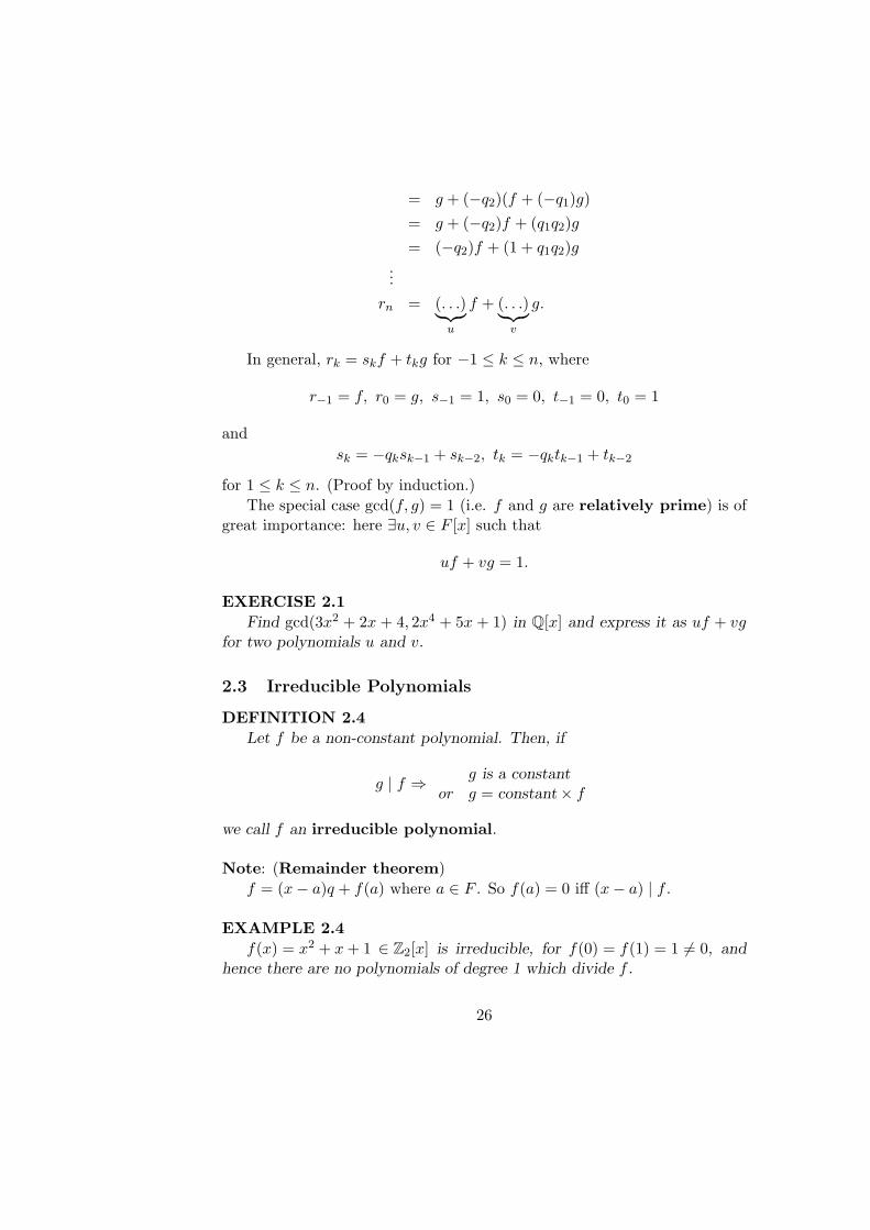
= g + (−q2)(f + (−q1)g)= g + (−q2)f + (q1q2)g= (−q2)f + (1 + q1q2)g

...rn = (. . .)︸︷︷︸

u

f + (. . .)︸︷︷︸v

g.

In general, rk = skf + tkg for −1 ≤ k ≤ n, where

r−1 = f, r0 = g, s−1 = 1, s0 = 0, t−1 = 0, t0 = 1

andsk = −qksk−1 + sk−2, tk = −qktk−1 + tk−2

for 1 ≤ k ≤ n. (Proof by induction.)The special case gcd(f, g) = 1 (i.e. f and g are relatively prime) is of

great importance: here ∃u, v ∈ F [x] such that

uf + vg = 1.

EXERCISE 2.1Find gcd(3x2 + 2x + 4, 2x4 + 5x + 1) in Q[x] and express it as uf + vg

for two polynomials u and v.

2.3 Irreducible Polynomials

DEFINITION 2.4Let f be a non-constant polynomial. Then, if

g | f ⇒ g is a constantor g = constant× f

we call f an irreducible polynomial.

Note: (Remainder theorem)f = (x− a)q + f(a) where a ∈ F . So f(a) = 0 iff (x− a) | f .

EXAMPLE 2.4f(x) = x2 + x+ 1 ∈ Z2[x] is irreducible, for f(0) = f(1) = 1 6= 0, and

hence there are no polynomials of degree 1 which divide f .

26

THEOREM 2.2Let f be irreducible. Then if f 6 | g, gcd(f, g) = 1 and ∃u, v ∈ F [x] such

that

uf + vg = 1.

PROOF Suppose f is irreducible and f 6 | g. Let d = gcd(f, g) so

d | f and d | g.

Then either d = cf for some constant c, or d = 1. But if d = cf then

f | d and d | g⇒ f | g —a contradiction.

So d = 1 as required.

COROLLARY 2.4If f is irreducible and f | gh, then f | g or f | h.

Proof: Suppose f is irreducible and f | gh, f 6 | g. We show that f | h.

By the above theorem, ∃u, v such that

uf + vg = 1⇒ ufh+ vgh = h

⇒ f | h

THEOREM 2.3Any non-constant polynomial is expressible as a product of irreducible

polynomials where representation is unique up to the order of the irreduciblefactors.

Some examples:

(x+ 1)2 = x2 + 2x+ 1= x2 + 1 inZ2[x]

(x2 + x+ 1)2 = x4 + x2 + 1 in Z2[x](2x2 + x+ 1)(2x+ 1) = x3 + x2 + 1 inZ3[x]

= (x2 + 2x+ 2)(x+ 2) inZ3[x].

PROOF

27

Existence of factorization: If f ∈ F [x] is not a constant polynomial, thenf being irreducible implies the result.

Otherwise, f = f1F1, with 0 < deg f1,degF1 < deg f . If f1 and F1 areirreducible, stop. Otherwise, keep going.

Eventually we end with a decomposition of f into irreducible poly-nomials.

Uniqueness: Letcf1f2 · · · fm = dg1g2 · · · gn

be two decompositions into products of constants (c and d) and monicirreducibles (fi, gj). Now

f1 | f1f2 · · · fm =⇒ f1 | g1g2 · · · gn

and since fi, gi are irreducible we can cancel f1 and some gj .

Repeating this for f2, . . . , fm, we eventually obtain m = n and c = d—in other words, each expression is simply a rearrangement of the factorsof the other, as required.

THEOREM 2.4Let Fq be a field with q elements. Then if n ∈ N, there exists an irred-

ucible polynomial of degree n in F [x].

PROOF First we introduce the idea of the Riemann zeta function:

ζ(s) =∞∑n=1

1ns

=∏

p prime

1

1− 1ps.

To see the equality of the latter expressions note that

11− x

=∞∑i=0

xi = 1 + x+ x2 + · · ·

and so

R.H.S. =∏

p prime

( ∞∑i=0

1pis

)

=(

1 +12s

+1

22s+ · · ·

)(1 +

13s

+1

32s+ · · ·

)= 1 +

12s

+13s

+14s

+ · · ·

28

—note for the last step that terms will be of form(1

pa11 · · · p

aRR

)sup to some prime pR, with ai ≥ 0 ∀i = 1, . . . , R. and as R→∞, the primefactorizations

pa11 · · · p

aRR

map onto the natural numbers, N.We let Nm denote the number of monic irreducibles of degree m in Fq[x].

For example, N1 = q since x+ a, a ∈ Fq are the irreducible polynomials ofdegree 1.

Now let |f | = qdeg f , and |0| = 0. Then we have

|fg| = |f | |g| since deg fg = deg f + deg g

and, because of the uniqueness of factorization theorem,∑f monic

1|f |s

=∏

f monic andirreducible

1

1− 1|f |s

.

Now the left hand side is

∞∑n=0

∑f monic anddeg f = n

1|f |s

=∞∑n=0

qn

qns

(there are qn monic polynomials of degree n)

=∞∑n=0

1qn(s−1)

=1

1− 1qs−1

and R.H.S. =∞∏n=1

1(1− 1

qns)Nn .29

Equating the two, we have

1

1− 1qs−1

=∞∏n=1

1(1− 1

qns)Nn . (4)

We now take logs of both sides, and then use the fact that

log(

11− x

)=∞∑n=1

xn

nif |x| < 1;

so (4) becomes

log1

1− q−(s−1)=

∞∏n=1

1(1− 1

qns)Nn

⇒∞∑k=1

1kq(s−1)k

= −∞∑n=1

Nn log(

1− 1qns

)

=∞∑n=1

Nn

∞∑m=1

1mqmns

so∞∑k=1

qk

kqsk=

∞∑n=1

Nn

∞∑m=1

n

mnqmns

=∞∑k=1

∑mn=k

nNn

kqks.

Putting x = qs, we have∞∑k=1

qkxk

k=∞∑k=1

xk ×∑mn=k

nNn,

and since both sides are power series, we may equate coefficients of xk toobtain

qk =∑mn=k

nNn =∑n|k

nNn. (5)

We can deduce from this that Nn > 0 as n→∞ (see Berlekamp’s “AlgebraicCoding Theory”).

Now note that N1 = q, so if k is a prime—say k = p, (5) gives

qp = N1 + pNp = q + pNp

⇒ Np =qp − qp

> 0 as q > 1 and p ≥ 2.

30

This proves the theorem for n = p, a prime.But what if k is not prime? Equation (5) also tells us that

qk ≥ kNk.

Now let k ≥ 2. Then

qk = kNk +∑n|kn6=k

nNn

≤ kNk +∑n|kn6=k

qn (as nNn ≤ qn)

≤ kNk +bk/2c∑n=1

qn

< kNk +bk/2c∑n=0

qn (adding 1)

= kNk +qbk/2c+1 − 1

q − 1(sum of geometric series).

Butqt+1 − 1q − 1

< qt+1 if q ≥ 2,

so

qk < kNk + qbk/2c+1

⇒ Nk >qk − qbk/2c+1

k

≥ 0 if qk ≥ qbk/2c+1.

Since q > 1 (we cannot have a field with a single element, since the additiveand multiplicative identities cannot be equal by one of the axioms), thelatter condition is equivalent to

k ≥ bk/2c+ 1

which is true and the theorem is proven.

31

2.4 Minimum Polynomial of a (Square) Matrix

Let A ∈Mn×n(F ), and g = chA . Then g(A) = 0 by the Cayley–Hamiltontheorem.

DEFINITION 2.5Any non–zero polynomial g of minimum degree and satisfying g(A) = 0

is called a minimum polynomial of A.

Note: If f is a minimum polynomial of A, then f cannot be a constantpolynomial. For if f = c, a constant, then 0 = f(A) = cIn implies c = 0.

THEOREM 2.5If f is a minimum polynomial of A and g(A) = 0, then f | g. (In partic-

ular, f | chA.)

PROOF Let g(A) = 0 and f be a minimum polynomial. Then

g = qf + r,

where r = 0 or deg r < deg f . Hence

g(A) = q(A)× 0 + r(A)0 = r(A).

So if r 6= 0, the inequality deg r < deg f would give a contradict the defini-tion of f . Consequently r = 0 and f | g.Note: It follows that if f and g are minimum polynomials of A, then f |gand g|f and consequently f = cg, where c is a scalar. Hence there is aunique monic minimum polynomial and we denote it by mA.

EXAMPLES (of minimum polynomials):

1. A = 0⇔ mA = x

2. A = In ⇔ mA = x− 1

3. A = cIn ⇔ mA = x− c

4. A2 = A and A 6= 0 and A 6= In ⇔ mA = x2 − x.

EXAMPLE 2.5F = Q and

A =

5 −6 −6−1 4 2

3 −6 −4

.32

Now

A 6= c0I3, c0 ∈ Q, so mA 6= x− c0,

A2 = 3A− 2I3

⇒ mA = x2 − 3x+ 2

This is an special case of a general algorithm:

(Minimum polynomial algorithm) Let A ∈Mn×n(F ). Then we find theleast positive integer r such that Ar is expressible as a linear combinationof the matrices

In, A, . . . , Ar−1,

sayAr = c0 + c1A+ · · ·+ cr−1A

r−1.

(Such an integer must exist as In, A, . . . , An2

form a linearly dependentfamily in the vector space Mn×n(F ) and this latter space has dimensionequal to n2.)

Then mA = xr − cr−1xr−1 − · · · − c1x− c0.

THEOREM 2.6If f = xn + an−1x

n−1 + · · ·+ a1x+ a0 ∈ F [x], then mC(f) = f , where

C(f) =

0 0 0 −a0

1 0 · · · 0 −a1

0 1 0 −a2...

. . ....

0 0 · · · 1 −an−1

.

PROOF For brevity denote C(f) by A. Then post-multiplying A by therespective unit column vectors E1, . . . , En gives

AE1 = E2

AE2 = E3 ⇒ A2E1 = E3

...AEn−1 = En ⇒ An−1E1 = En

AEn = −a0E1 − a2E2 − · · · − an−1En

= −a0E1 − a2AE1 − · · · − an−1An−1E1 = AnE1,

33

so⇒ f(A)E1 = 0⇒ first column of f(A) zero

Now although matrix multiplication is not commutative, multiplication oftwo matrices, each of which is a polynomial in a given square matrix A, iscommutative. Hence f(A)g(A) = g(A)f(A) if f, g ∈ F [x]. Taking g = xgives

f(A)A = Af(A).

Thusf(A)E2 = f(A)AE1 = Af(A)E1 = 0

and so the second column of A is zero. Repeating this for E3, . . . , En, wesee that

f(A) = 0

and thus mA|f .To show mA = f , we assume degmA = t < n; say

mA = xt + bt−1xt−1 + · · ·+ b0.

Now

mA(A) = 0⇒ At + bt−1A

t−1 + · · ·+ b0In = 0⇒ (At + bt−1A

t−1 + · · ·+ b0In)E1 = 0,

and recalling that AE1 = E2 etc., and t < n, we have

Et+1 + bt−1Et + · · ·+ b1E2 + b0E1 = 0

which is a contradiction—since the Ei are independent, the coefficient ofEt+1 cannot be 1.

Hence mA = f .Note: It follows that chA = f . Because both chA and mA have degree nand moreover mA divides chA .

EXERCISE 2.2If A = Jn(a) for a ∈ F , an elementary Jordan matrix of size n, show

34

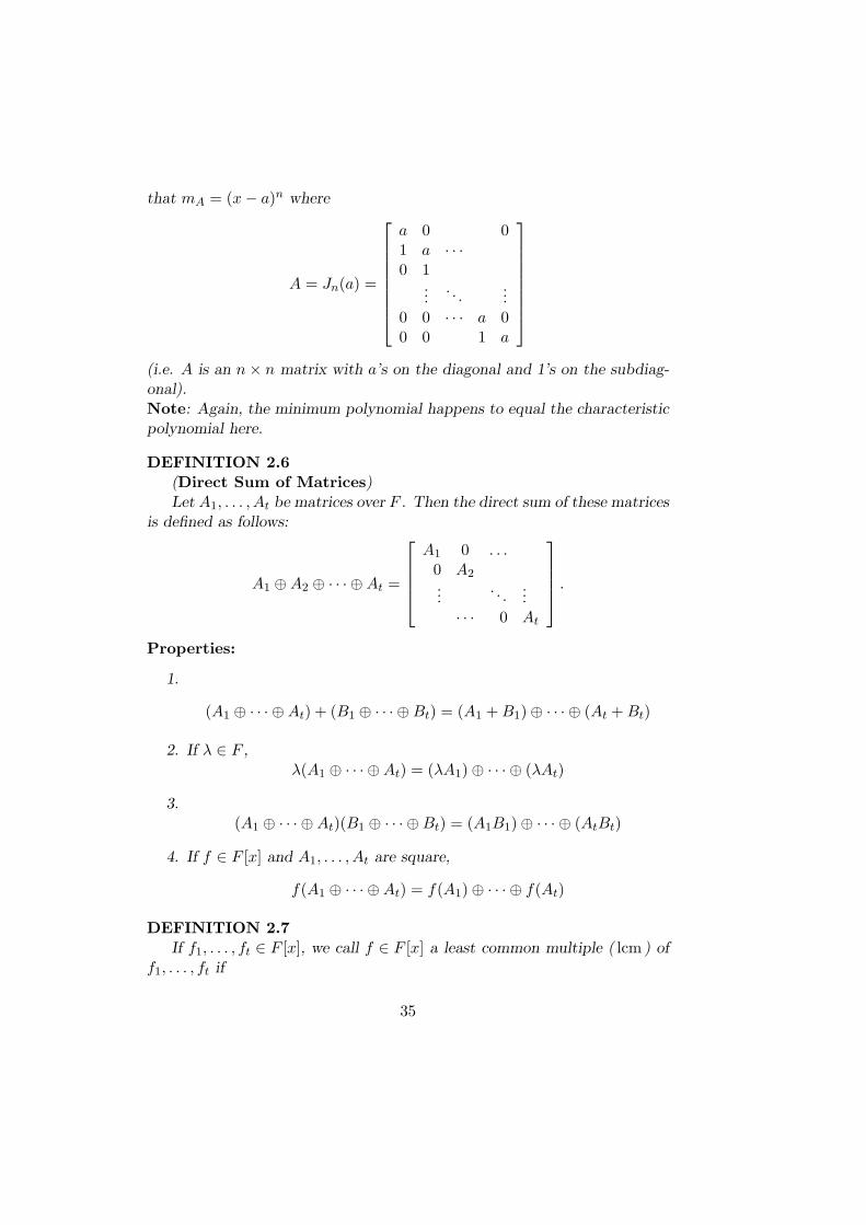
that mA = (x− a)n where

A = Jn(a) =

a 0 01 a · · ·0 1

.... . .

...0 0 · · · a 00 0 1 a

(i.e. A is an n× n matrix with a’s on the diagonal and 1’s on the subdiag-onal).Note: Again, the minimum polynomial happens to equal the characteristicpolynomial here.

DEFINITION 2.6(Direct Sum of Matrices)Let A1, . . . , At be matrices over F . Then the direct sum of these matrices

is defined as follows:

A1 ⊕A2 ⊕ · · · ⊕At =

A1 0 . . .

0 A2...

. . ....

· · · 0 At

.Properties:

1.

(A1 ⊕ · · · ⊕At) + (B1 ⊕ · · · ⊕Bt) = (A1 +B1)⊕ · · · ⊕ (At +Bt)

2. If λ ∈ F ,λ(A1 ⊕ · · · ⊕At) = (λA1)⊕ · · · ⊕ (λAt)

3.(A1 ⊕ · · · ⊕At)(B1 ⊕ · · · ⊕Bt) = (A1B1)⊕ · · · ⊕ (AtBt)

4. If f ∈ F [x] and A1, . . . , At are square,

f(A1 ⊕ · · · ⊕At) = f(A1)⊕ · · · ⊕ f(At)

DEFINITION 2.7If f1, . . . , ft ∈ F [x], we call f ∈ F [x] a least common multiple ( lcm ) of

f1, . . . , ft if

35

1. f1 | f, . . . ft | f , and

2. f1 | e, . . . ft | e⇒ f | e.

This uniquely defines the lcm up to a constant multiple and so we set “the”lcm to be the monic lcm .

EXAMPLES 2.1

If fg 6= 0, lcm (f, g) | fg .

(Recursive property)

lcm (f1, . . . , ft+1) = lcm ( lcm (f1, . . . , ft), ft+1).

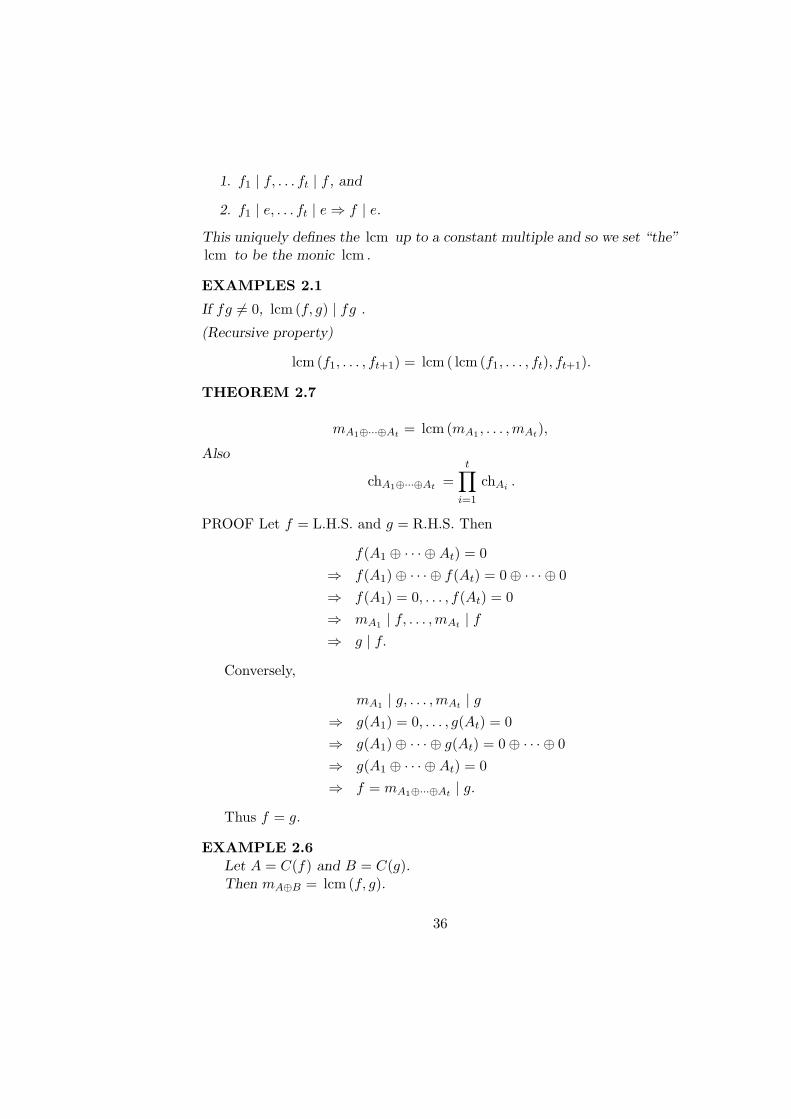
THEOREM 2.7

mA1⊕···⊕At = lcm (mA1 , . . . ,mAt),

Also

chA1⊕···⊕At =t∏i=1

chAi .

PROOF Let f = L.H.S. and g = R.H.S. Then

f(A1 ⊕ · · · ⊕At) = 0⇒ f(A1)⊕ · · · ⊕ f(At) = 0⊕ · · · ⊕ 0⇒ f(A1) = 0, . . . , f(At) = 0⇒ mA1 | f, . . . ,mAt | f⇒ g | f.

Conversely,

mA1 | g, . . . ,mAt | g⇒ g(A1) = 0, . . . , g(At) = 0⇒ g(A1)⊕ · · · ⊕ g(At) = 0⊕ · · · ⊕ 0⇒ g(A1 ⊕ · · · ⊕At) = 0⇒ f = mA1⊕···⊕At | g.

Thus f = g.

EXAMPLE 2.6Let A = C(f) and B = C(g).Then mA⊕B = lcm (f, g).

36

Note: If

f = cpa11 . . . patt

g = dpb11 . . . pbtt

where c, d 6= 0 are in F and p1, . . . , pt are distinct monic irreducibles, then

gcd(f, g) = pmin(a1,b1)1 . . . p

min(at,bt)t ,

lcm (f, g) = pmax(a1,b1)1 . . . p

max(at,bt)t

Note

min(ai, bi) + max(ai, bi) = ai + bi.

so

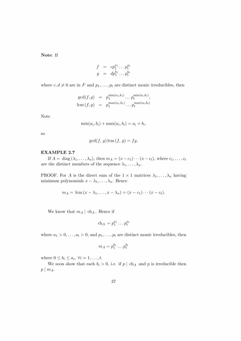
gcd(f, g) lcm (f, g) = fg.

EXAMPLE 2.7If A = diag (λ1, . . . , λn), then mA = (x− c1) · · · (x− ct), where c1, . . . , ct

are the distinct members of the sequence λ1, . . . , λn.

PROOF. For A is the direct sum of the 1 × 1 matrices λ1, . . . , λn havingminimum polynomials x− λ1, . . . , λn. Hence

mA = lcm (x− λ1, . . . , x− λn) = (x− c1) · · · (x− ct).

We know that mA | chA . Hence if

chA = pa11 . . . patt

where a1 > 0, . . . , at > 0, and p1, . . . , pt are distinct monic irreducibles, then

mA = pb11 . . . pbtt

where 0 ≤ bi ≤ ai, ∀i = 1, . . . , t.We soon show that each bi > 0, i.e. if p | chA and p is irreducible then

p | mA.

37

2.5 Construction of a field of pn elements

(where p is prime and n ∈ N)

Let f be a monic irreducible polynomial of degree n in Zp[x]—that is,Fq = Zp here.For instance,

n = 2, p = 2 ⇒ x2 + x+ 1 = f

n = 3, p = 2 ⇒ x3 + x+ 1 = f or x3 + x2 + 1 = f.

Let A = C(f), the companion matrix of f . Then we know f(A) = 0.We assert that the set of all matrices of the form g(A), where g ∈ Zp[x],

forms a field consisting of precisely pn elements. The typical element is

b0In + b1A+ · · ·+ btAt

where b0, . . . , bt ∈ Zp.We need only show existence of a multiplicative inverse for each element

except 0 (the additive identity), as the remaining axioms clearly hold.So let g ∈ Zp[x] such that g(A) 6= 0. We have to find h ∈ Zp[x] satisfying

g(A)h(A) = In.

Note that g(A) 6= 0⇒ f 6 | g, since

f | g ⇒ g = ff1

and henceg(A) = f(A)f1(A) = 0f1(A) = 0.

Then since f is irreducible and f 6 | g, there exist u, v ∈ Zp[x] such that

uf + vg = 1.

Hence u(A)f(A) + v(A)g(A) = In and v(A)g(A) = In, as required.We now show that our new field is a Zp–vector space with basis consisting

of the matricesIn, A, . . . , A

n−1.

Firstly the spanning property: By Euclid’s division theorem,

g = fq + r

38

where q, r ∈ Zp[x] and deg r < deg g. So let

r = r0 + r1x+ · · ·+ rn−1xn−1

where r0, . . . , rn−1 ∈ Zp. Then

g(A) = f(A)q(A) + r(A)= 0q(A) + r(A)= r(A)= r0In + r1A+ · · ·+ rn−1A

n−1

Secondly, linear independence over Zp: Suppose that

r0In + r1A+ · · ·+ rn−1An−1 = 0,

where r0, r1, . . . , rn−1 ∈ Zp. Then r(A) = 0, where

r = r0 + r1x+ · · ·+ rn−1xn−1.

Hence mA = f divides r. Consequently r = 0, as deg f = n whereasdeg r < n if r 6= 0.

Consequently, there are pn such matrices g(A) in the field we have con-structed.

Numerical Examples

EXAMPLE 2.8Let p = 2, n = 2, f = x2 + x+ 1 ∈ Z2[x], and A = C(f). Then

A =[

0 −11 −1

]=[

0 11 1

],

and

F4 = { a0I2 + a1A | a0, a1 ∈ Z2 }= { 0, I2, A, I2 +A }.

We construct addition and multiplication tables for this field, with B =I2 +A (as an exercise, check these):

⊕ 0 I2 A B

0 0 I2 A B

I2 I2 0 B A

A A B 0 I2

B B A I2 0

⊗ 0 I2 A B

0 0 0 0 0I2 0 I2 A B

A 0 A B I2

B 0 B I2 A

39

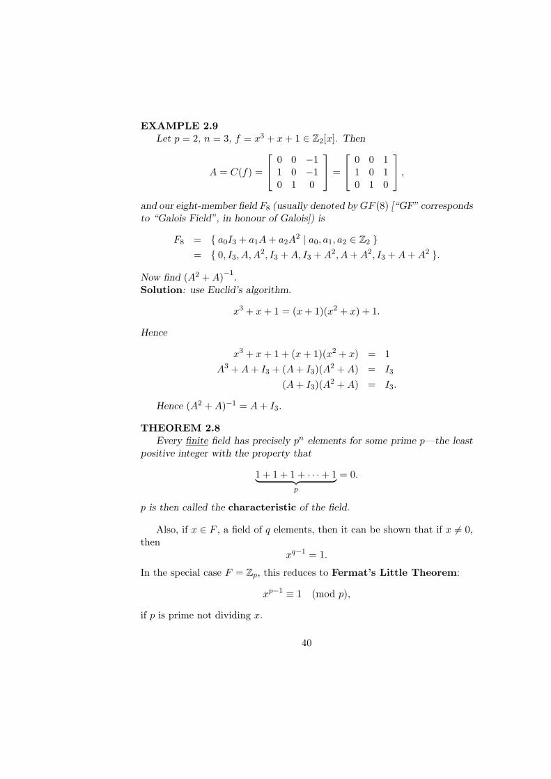
EXAMPLE 2.9Let p = 2, n = 3, f = x3 + x+ 1 ∈ Z2[x]. Then

A = C(f) =

0 0 −11 0 −10 1 0

=

0 0 11 0 10 1 0

,and our eight-member field F8 (usually denoted byGF (8) [“GF” correspondsto “Galois Field”, in honour of Galois]) is

F8 = { a0I3 + a1A+ a2A2 | a0, a1, a2 ∈ Z2 }

= { 0, I3, A,A2, I3 +A, I3 +A2, A+A2, I3 +A+A2 }.

Now find (A2 +A)−1.

Solution: use Euclid’s algorithm.

x3 + x+ 1 = (x+ 1)(x2 + x) + 1.

Hence

x3 + x+ 1 + (x+ 1)(x2 + x) = 1A3 +A+ I3 + (A+ I3)(A2 +A) = I3

(A+ I3)(A2 +A) = I3.

Hence (A2 +A)−1 = A+ I3.

THEOREM 2.8Every finite field has precisely pn elements for some prime p—the least

positive integer with the property that

1 + 1 + 1 + · · ·+ 1︸ ︷︷ ︸p

= 0.

p is then called the characteristic of the field.

Also, if x ∈ F , a field of q elements, then it can be shown that if x 6= 0,then

xq−1 = 1.

In the special case F = Zp, this reduces to Fermat’s Little Theorem:

xp−1 ≡ 1 (mod p),

if p is prime not dividing x.

40

2.6 Characteristic and Minimum Polynomial of a Transform-ation

DEFINITION 2.8(Characteristic polynomial of T : V 7→ V )

Let β be a basis for V and A = [T ]ββ.Then we define chT = chA . This polynomial is independent of the basis

β:

PROOF ( chT is independent of the basis.)If γ is another basis for V and B = [T ]γγ , then we know A = P−1BP

where P is the change of basis matrix [IV ]γβ .Then

chA = chP−1BP

= det(xIn − P−1BP ) where n = dimV

= det(P−1(xIn)P − P−1BP )= det(P−1(xIn −B)P )= detP−1 chB detP= chB .

DEFINITION 2.9If f = a0 + · · ·+ atx

t, where a0, . . . , at ∈ F , we define

f(T ) = a0IV + · · ·+ atTt.

Then the usual properties hold:

f, g ∈ F [x]⇒ (f+g)(T ) = f(T )+g(T ) and (fg)(T ) = f(T )g(T ) = g(T )f(T ).

LEMMA 2.1

f ∈ F [x]⇒ [f(T )]ββ = f(

[T ]ββ).

Note: The Cayley-Hamilton theorem for matrices says that chA (A) = 0.Then if A = [T ]ββ, we have by the lemma

[ chT (T )]ββ = chT (A) = chA (A) = 0,

so chT (T ) = 0V .

41

DEFINITION 2.10Let T : V → V be a linear transformation over F . Then any polynomial

of least positive degree such that

f(T ) = 0V

is called a minimum polynomial of T .

We have corresponding results for polynomials in a transformation T tothose for polynomials in a square matrix A:

g = qf + r ⇒ g(T ) = q(T )f(T ) + r(T ).

Again, there is a unique monic minimum polynomial of T is denoted by mT

and called “the” minimum polynomial of T .Also note that because of the lemma,

mT = m[T ]ββ

.

For (with A = [T ]ββ)

(a) mA(A) = 0, so mA(T ) = 0V . Hence mT |mA.

(b) mT (T ) = 0V , so [mT (T )]ββ = 0. Hence mT (A) = 0 and so mA|mT .

EXAMPLES 2.2

T = 0V ⇔ mT = x.

T = IV ⇔ mT = x− 1.

T = cIV ⇔ mT = x− c.T 2 = T and T 6= 0V and T 6= IV ⇔ mT = x2 − x.

2.6.1 Mn×n(F [x])—Ring of Polynomial Matrices

Example: [x2 + 2 x5 + 5x+ 1x+ 3 1

]∈M2×2(Q[x])

= x5

[0 10 0

]+ x2

[1 00 0

]+ x

[0 51 0

]+[

2 13 1

]—we see that any element of Mn×n(F [x]) is expressible as

xmAm + xm−1Am−1 + · · ·+A0

where Ai ∈Mn×n(F ). We write the coefficient of xi after xi, to distinguishthese entities from corresponding objects of the following ring.

42

2.6.2 Mn×n(F )[y]—Ring of Matrix Polynomials

This consists of all polynomials in y with coefficients in Mn×n(F ).Example:[

0 10 0

]y5 +

[1 00 0

]y2 +

[0 51 0

]y +

[2 13 1

]∈M2×2(F )[y].

THEOREM 2.9The mapping

Φ : Mn×n(F )[y] 7→Mn×n(F [x])

given by

Φ(A0 +A1y + · · ·+Amym) = A0 + xA1 + · · ·+ xmAm

where Ai ∈Mn×n(F ), is a 1–1 correspondence and has the following prop-erties:

Φ(X + Y ) = Φ(X) + Φ(Y )Φ(XY ) = Φ(X)Φ(Y )Φ(tX) = tΦ(X) ∀t ∈ F.

AlsoΦ(Iny −A) = xIn −A ∀A ∈Mn×n(F ).

THEOREM 2.10 ((Left) Remainder theorem for matrix polynomials)

Let Bmym + · · ·+B0 ∈Mn×n(F )[y] and A ∈Mn×n(F ).

ThenBmy

m + · · ·+B0 = (Iny −A)Q+R

where

R = AmBm + · · ·+AB1 +B0

and Q = Cm−1ym−1 + · · ·+ C0

where Cm−1, . . . , C0 are computed recursively:

Bm = Cm−1

Bm−1 = −ACm−1 + Cm−2

...

B1 = −AC1 + C0.

43

PROOF. First we verify that B0 = −AC0 +R:

R = AmBm = AmCm−1

+Am−1Bm−1 −AmCm−1 +Am−1Cm−2

+ +...

...+AB1 −A2C1 +AC0

+B0 B0

= B0 +AC0.

Then

(Iny −A)Q+R = (Iny)(Cm−1ym−1 + · · ·+ C0)

−A(Cm−1ym−1 + · · ·+ C0) +AmBm + · · ·+B0

= Cm−1ym + (Cm−2 −ACm−1)ym−1 + · · ·+ (C0 −AC1)y +

−AC0 +R

= Bmym +Bm−1y

m−1 + · · ·+B1y +B0.

Remark. There is a similar “right” remainder theorem.

THEOREM 2.11If p is an irreducible polynomial dividing chA , then p | mA.

PROOF (From Burton Jones, ”Linear Algebra”).Let mA = xt + at−1x

t−1 + · · ·+ a0 and consider the matrix polynomialin y

Φ−1(mAIn) = Inyt + (at−1In)yt−1 + · · ·+ (a0In)

= (Iny −A)Q+AtIn +At−1(at−1In) + · · ·+ a0In

= (Iny −A)Q+mT (A)= (Iny −A)Q.

Now take Φ of both sides to give

mAIn = (xIn −A)Φ(Q)

and taking determinants of both sides yields

{mA}n = chA × det Φ(Q).

44

So letting p be an irreducible polynomial dividing chA , we have p | {mA}nand hence p | mA.

Alternative simpler proof (MacDuffee):mA(x)−mA(y) = (x− y)k(x, y), where k(x, y) ∈ F [x, y]. Hence

mA(x)In = mA(xIn)−mA(A) = (xIn −A)k(xIn, A).

Now take determinants to get

mA(x)n = chA(x) det k(xIn, A).

Exercise: If ∆(x) is the gcd of the elements of adj(xIn − A), use theequation (xIn−a)adj(xIn−A) = chA(x)In and an above equation to deducethat mA(x) = chA(x)/∆(x).

EXAMPLES 2.3

With A = 0 ∈Mn×n(F ), we have chA = xn and mA = x.

A = diag (1, 1, 2, 2, 2) ∈M5×5(Q). Here

chA = (x− 1)2(x− 2)3 and mA = (x− 1)(x− 2).

DEFINITION 2.11A matrix A ∈ Mn×n(F ) is called diagonable over F if there exists a

non–singular matrix P ∈Mn×n(F ) such that

P−1AP = diag (λ1, . . . , λn),

where λ1, . . . , λn belong to F .

THEOREM 2.12If A is diagonable, then mA is a product of distinct linear factors.

PROOFIf P−1AP = diag (λ1, . . . , λn) (with λ1, . . . , λn ∈ F ) then

mA = mP−1AP = mdiag (λ1, . . . , λn)

= (x− c1)(x− c2) . . . (x− ct)

where c1, . . . , ct are the distinct members of the sequence λ1, . . . , λn.The converse is also true, and will (fairly) soon be proved.

45

EXAMPLE 2.10

A = Jn(a).

We saw earlier that mA = (x− a)n so if n ≥ 2 we see that A is not diago-nable.

DEFINITION 2.12(Diagonable LTs)

T : V 7→ V is called diagonable over F if there exists a basis β for Vsuch that [T ]ββ is diagonal.

THEOREM 2.13A is diagonable ⇔ TA is diagonable.

PROOF (Sketch)

⇒ Suppose P−1AP = diag (λ1, . . . , λn). Now pre-multiplying by P andletting P = [P1| · · · |Pn] we see that

TA(P1) = AP1 = λ1P1

...TA(Pn) = APn = λnPn

and we let β be the basis P1, . . . , Pn over Vn(F ). Then

[TA]ββ =

λ1

λ2

. . .λn

.

⇐ Reverse the argument and use Theorem 1.17.

THEOREM 2.14Let A ∈ Mn×n(F ). Then if λ is an eigenvalue of A with multiplicity m,

(that is (x− λ)m is the exact power of x− λ which divides chA ), we have

nullity (A− λIn) ≤ m.

46

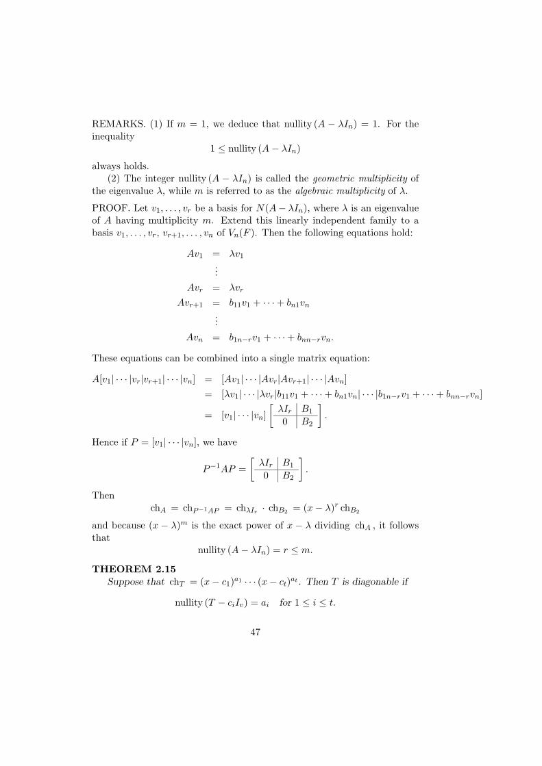
REMARKS. (1) If m = 1, we deduce that nullity (A − λIn) = 1. For theinequality

1 ≤ nullity (A− λIn)

always holds.(2) The integer nullity (A − λIn) is called the geometric multiplicity of

the eigenvalue λ, while m is referred to as the algebraic multiplicity of λ.

PROOF. Let v1, . . . , vr be a basis for N(A− λIn), where λ is an eigenvalueof A having multiplicity m. Extend this linearly independent family to abasis v1, . . . , vr, vr+1, . . . , vn of Vn(F ). Then the following equations hold:

Av1 = λv1

...Avr = λvr

Avr+1 = b11v1 + · · ·+ bn1vn...

Avn = b1n−rv1 + · · ·+ bnn−rvn.

These equations can be combined into a single matrix equation:

A[v1| · · · |vr|vr+1| · · · |vn] = [Av1| · · · |Avr|Avr+1| · · · |Avn]= [λv1| · · · |λvr|b11v1 + · · ·+ bn1vn| · · · |b1n−rv1 + · · ·+ bnn−rvn]

= [v1| · · · |vn][λIr B1

0 B2

].

Hence if P = [v1| · · · |vn], we have

P−1AP =[λIr B1

0 B2

].

ThenchA = chP−1AP = chλIr · chB2 = (x− λ)r chB2

and because (x − λ)m is the exact power of x − λ dividing chA , it followsthat

nullity (A− λIn) = r ≤ m.

THEOREM 2.15Suppose that chT = (x− c1)a1 · · · (x− ct)at . Then T is diagonable if

nullity (T − ciIv) = ai for 1 ≤ i ≤ t.

47

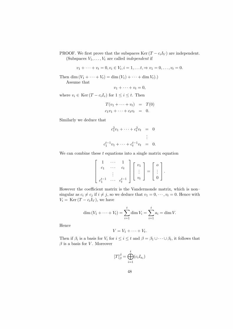
PROOF. We first prove that the subspaces Ker (T − ciIV ) are independent.(Subspaces V1, . . . , Vt are called independent if

v1 + · · ·+ vt = 0, vi ∈ Vi, i = 1, . . . t,⇒ v1 = 0, . . . , vt = 0.

Then dim (V1 + · · ·+ Vt) = dim (V1) + · · ·+ dimVt).)Assume that

v1 + · · ·+ vt = 0,

where vi ∈ Ker (T − ciIv) for 1 ≤ i ≤ t. Then

T (v1 + · · ·+ vt) = T (0)c1v1 + · · ·+ ctvt = 0.

Similarly we deduce that

c21v1 + · · ·+ c2

t vt = 0...

ct−11 v1 + · · ·+ ct−1

t vt = 0.

We can combine these t equations into a single matrix equation1 · · · 1c1 · · · ct

...ct−1

1 · · · ct−1t

v1

...vt

=

o...0

.However the coefficient matrix is the Vandermonde matrix, which is non–singular as ci 6= cj if i 6= j, so we deduce that v1 = 0, · · · , vt = 0. Hence withVi = Ker (T − ciIV ), we have

dim (V1 + · · ·+ Vt) =t∑i=1

dimVi =t∑i=1

ai = dimV.

HenceV = V1 + · · ·+ Vt.

Then if βi is a basis for Vi for i ≤ i ≤ t and β = β1 ∪ · · · ∪ βt, it follows thatβ is a basis for V . Moreover

[T ]ββ =t⊕i=1

(ciIai)

48

and T is diagonable.

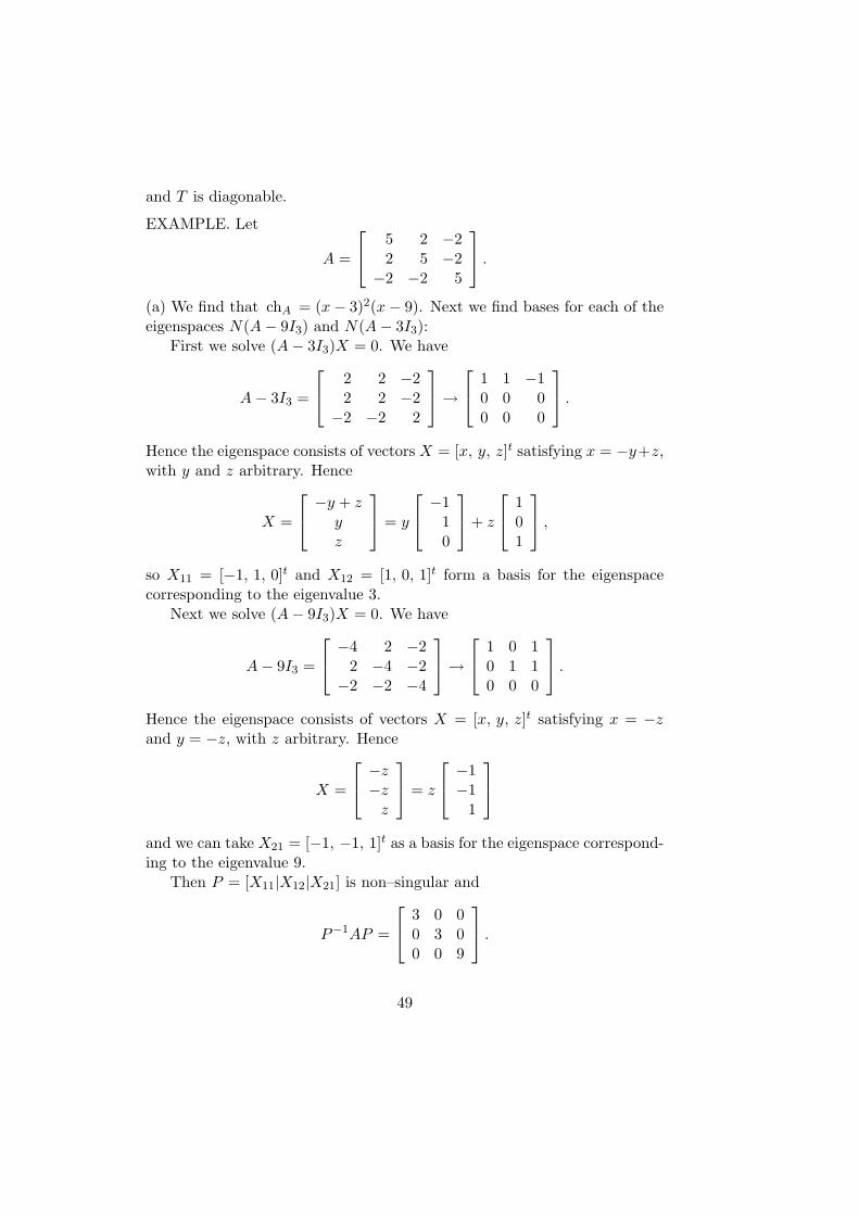
EXAMPLE. Let

A =

5 2 −22 5 −2−2 −2 5

.(a) We find that chA = (x− 3)2(x− 9). Next we find bases for each of theeigenspaces N(A− 9I3) and N(A− 3I3):

First we solve (A− 3I3)X = 0. We have

A− 3I3 =

2 2 −22 2 −2−2 −2 2

→ 1 1 −1

0 0 00 0 0

.Hence the eigenspace consists of vectors X = [x, y, z]t satisfying x = −y+z,with y and z arbitrary. Hence

X =

−y + zyz

= y

−110

+ z

101

,so X11 = [−1, 1, 0]t and X12 = [1, 0, 1]t form a basis for the eigenspacecorresponding to the eigenvalue 3.

Next we solve (A− 9I3)X = 0. We have

A− 9I3 =

−4 2 −22 −4 −2−2 −2 −4

→ 1 0 1

0 1 10 0 0

.Hence the eigenspace consists of vectors X = [x, y, z]t satisfying x = −zand y = −z, with z arbitrary. Hence

X =

−z−zz

= z

−1−1

1

and we can take X21 = [−1, −1, 1]t as a basis for the eigenspace correspond-ing to the eigenvalue 9.

Then P = [X11|X12|X21] is non–singular and

P−1AP =

3 0 00 3 00 0 9

.49

THEOREM 2.16If

mT = (x− c1) . . . (x− ct)

for c1, . . . , ct distinct in F , then T is diagonable and conversely. Moreoverthere exist unique linear transformations T1, . . . , Tt satisfying

IV = T1 + · · ·+ Tt,

T = c1T1 + · · ·+ ctTt,

TiTj = 0V if i 6= j,

T 2i = Ti, 1 ≤ i ≤ t.

Also rankTi = ai, where chT = (x− c1)a1 · · · (x− ct)at .

Remarks.

1. T1, . . . , Tt are called the principal idempotents of T .

2. If g ∈ F [x], then g(T ) = g(c1)T1 + · · ·+ g(ct)Tt. For example

Tm = cm1 T1 + · · ·+ cmt Tt.

3. If c1, . . . , ct are non–zero (that is the eigenvalues of T are non–zero),the T−1 is given by

T−1 = c−11 T1 + · · ·+ c−1

t Tt.

Formulae 2 and 3 are useful in the corresponding matrix formulation. PROOFSuppose mT = (x − c1) · · · (x − ct), where c1, . . . , ct are distinct. ThenchT = (x − c1)a1 · · · (x − ct)at . To prove T is diagonable, we have to provethat nullity (T − ciIV ) = ai, 1 ≤ i ≤ t

Let p1, . . . , pt be the Lagrange interpolation polynomials based on c1, . . . , ct,i.e.

pi =t∏

j=1j 6=i

(x− cjci − cj

), 1 ≤ i ≤ t.

Theng ∈ F [x]⇒ g = g(c1)p1 + · · ·+ g(ct)pt.

In particular,g = 1⇒ 1 = p1 + · · ·+ pt

50

andg = x⇒ x = c1p1 + · · ·+ ctpt.

Hence with Ti = pi(T ),

IV = T1 + · · ·+ Tt

T = c1T1 + · · ·+ ctTt.

Next

mT = (x− c1) . . . (x− ct) | pipj if i 6= j

⇒ (pipj)(T ) = 0V if i 6= j

⇒ pi(T )pj(T ) = 0V or TiTj = 0V if i 6= j.

Then T 2i = Ti(T1 + · · ·+ Tt) = TiIV = Ti.

Next0V = mT (T ) = (T − c1IV ) · · · (T − ctIV ).

Hence

dimV = nullity 0V ≤t∑i=1

nullity (T − ciIV ) ≤t∑i=1

ai = dimV.

Consequently nullity (T − ciIV ) = ai, 1 ≤ i ≤ t and T is therefore diago-nable.

Next we prove that rankTi = ai. From the definition of pi, we have

nullity pi(T ) ≤t∑

j=1j 6=i

nullity (T − cjIV ) =t∑

j=1j 6=i

aj = dimV − ai.

Also pi(T )(T − ciIV ) = 0, so Im (T − ciIV ) ⊆ Ker pi(T ). Hence

dimV − ai ≤ nullity pi(T )

and consequently nullity pi(T ) = dim (V )− ai, so rank pi(T ) = ai.We next prove the uniqueness of T1, . . . , Tt. Suppose that S1, . . . , St also

satisfy the same conditions as T1, . . . , Tt. Then

TiT = TTi = ciTi

SjT = TSj = cjSj

Ti(TSj) = Ti(cjSj) = cjTiSj = (TiT )Sj = ciTiSj

51

so (cj − ci)TiSj = 0V and TiSj = 0V if i 6= j. Hence

Ti = TiIV = Ti(t∑

j=1

Sj) = TiSi

Si = IV Si = (t∑

j=1

Tj)Si = TiSi.

Hence Ti = Si.Conversely, suppose that T is diagonable and let β be a basis of V such

thatA = [T ]ββ = diag (λ1, . . . , λn).

Then mT = mA = (x − c1) · · · (x − ct), where c1, . . . , ct are the distinctmembers of the sequence λ1, . . . , λn.

COROLLARY 2.5If

chT = (x− c1) . . . (x− ct)with ci distinct members of F , then T is diagonable.Proof: Here mT = chT and we use theorem 3.3.

EXAMPLE 2.11Let

A =[

0 ab 0

]a, b ∈ F, ab 6= 0, 1 + 1 6= 0.

Then A is diagonable if and only if ab = y2 for some y ∈ F .For chA = x2 − ab, so if ab = y2,

chA = x2 − y2 = (x+ y)(x− y)

which is a product of distinct linear factors, as y 6= −y here.Conversely suppose that A is diagonable. Then as A is not a scalar

matrix, it follows that mA is not linear and hence

mA = (x− c1)(x− c2),

where c1 6= c2. Also chA = mA, so chA (c1) = 0. Hence

c21 − ab = 0, or ab = c2

1.

For example, take F = Z7 and let a = 1 and b = 3. Then ab 6= y2 andconsequently A is not diagonable.

52