2 lsst system design - welcome | the large … · 2 lsst system design john r ... space of possible...

2 LSST System Design

John R. Andrew, J. Roger P. Angel, Tim S. Axelrod, Jeffrey D. Barr, James G. Bartlett, JacekBecla, James H. Burge, David L. Burke, Srinivasan Chandrasekharan, David Cinabro, Charles F.Claver, Kem H. Cook, Francisco Delgado, Gregory Dubois-Felsmann, Eduardo E. Figueroa, JamesS. Frank, John Geary, Kirk Gilmore, William J. Gressler, J. S. Haggerty, Edward Hileman, ZeljkoIvezic, R. Lynne Jones, Steven M. Kahn, Jeff Kantor, Victor L. Krabbendam, Ming Liang, R. H.Lupton, Brian T. Meadows, Michelle Miller, David Mills, David Monet, Douglas R. Neill, MartinNordby, Paul O’Connor, John Oliver, Scot S. Olivier, Philip A. Pinto, Bogdan Popescu, VeljkoRadeka, Andrew Rasmussen, Abhijit Saha, Terry Schalk, Rafe Schindler, German Schumacher,Jacques Sebag, Lynn G. Seppala, M. Sivertz, J. Allyn Smith, Christopher W. Stubbs, Donald W.Sweeney, Anthony Tyson, Richard Van Berg, Michael Warner, Oliver Wiecha, David Wittman

This chapter covers the basic elements of the LSST system design, with particular emphasis onthose elements that may affect the scientific analyses discussed in subsequent chapters. We startwith a description of the planned observing strategy in § 2.1, and then go on to describe the keytechnical aspects of system, including the choice of site (§ 2.2), the telescope and optical design(§ 2.3), and the camera including the characteristics of its sensors and filters (§ 2.4). The keyelements of the data management system are described in § 2.5, followed by overviews of theprocedures that will be invoked to achieve the desired photometric (§ 2.6) and astrometric (§ 2.7)calibration.

2.1 The LSST Observing Strategy

Zeljko Ivezic, Philip A. Pinto, Abhijit Saha, Kem H. Cook

The fundamental basis of the LSST concept is to scan the sky deep, wide, and fast with a singleobserving strategy, giving rise to a data set that simultaneously satisfies the majority of the sciencegoals. This concept, the so-called “universal cadence,” will yield the main deep-wide-fast survey(typical single visit depth of r ∼ 24.5) and use about 90% of the observing time. The remaining10% of the observing time will be used to obtain improved coverage of parameter space such asvery deep (r ∼ 26) observations, observations with very short revisit times (∼ 1 minute), andobservations of “special” regions such as the ecliptic, Galactic plane, and the Large and SmallMagellanic Clouds. We are also considering a third type of survey, micro-surveys, that would useabout 1% of the time, or about 25 nights over ten years.

The observing strategy for the main survey will be optimized for the homogeneity of depth andnumber of visits over 20,000 deg2 of sky, where a “visit” is defined as a pair of 15-second exposures,performed back-to-back in a given filter, and separated by a four-second interval for readout andopening and closing of the shutter. In times of good seeing and at low airmass, preference is

25

Chapter 2: LSST System Design

given to r-band and i-band observations, as these are the bands in which the most seeing-sensitivemeasurements are planned. As often as possible, each field will be observed twice, with visitsseparated by 15-60 minutes. This strategy will provide motion vectors to link detections of movingobjects, and fine-time sampling for measuring short-period variability. The ranking criteria alsoensure that the visits to each field are widely distributed in position angle on the sky and rotationangle of the camera in order to minimize systematics that could affect some sensitive analyses,such as studies of cosmic shear.

The universal cadence will also provide the primary data set for the detection of near-Earth Ob-jects (NEO), given that it naturally incorporates the southern half of the ecliptic. NEO surveycompleteness for the smallest bodies (∼ 140 m in diameter per the Congressional NEO mandate1)is greatly enhanced, however, by the addition of a crescent on the sky within 10◦ of the northernecliptic. Thus, the “northern Ecliptic proposal” extends the universal cadence to this region usingthe r and i filters only, along with more relaxed limits on airmass and seeing. Relaxed limitson airmass and seeing are also adopted for ∼ 700 deg2 around the South Celestial pole, allowingcoverage of the Large and Small Magellanic Clouds.

Finally the universal cadence proposal excludes observations in a region of 1,000 deg2 aroundthe Galactic Center, where the high stellar density leads to a confusion limit at much brightermagnitudes than those attained in the rest of the survey. Within this region, the Galactic Centerproposal provides 30 observations in each of the six filters, distributed roughly logarithmically intime (it may not be necessary to use the bluest u and g filters for this heavily extincted region).The resulting sky coverage for the LSST baseline cadence, based on detailed operations simulationsdescribed in § 3.1, is shown for the r band in Figure 2.1. The anticipated total number of visitsfor a ten-year LSST survey is about 2.8 million (∼ 5.6 million 15-second long exposures). Theper-band allocation of these visits is shown in Table 1.1.

Although the uniform treatment of the sky provided by the universal cadence proposal can satisfythe majority of LSST scientific goals, roughly 10% of the time may be allocated to other strategiesthat significantly enhance the scientific return. These surveys aim to extend the parameter spaceaccessible to the main survey by going deeper or by employing different time/filter sampling.

In particular, we plan to observe a set of “deep drilling fields,” whereby one hour of observingtime per night is devoted to the observation of a single field to substantially greater depth inindividual visits. Accounting for read-out time and filter changes, about 50 consecutive 15-secondexposures could be obtained in each of four filters in an hour. This would allow us to measure lightcurves of objects on hour-long timescales, and detect faint supernovae and asteroids that cannotbe studied with deep stacks of data taken with a more spread-out cadence. The number, location,and cadence of these deep drilling fields are the subject of active discussion amongst the LSSTScience Collaborations; see for example the plan suggested by the Galaxies Science Collaborationat § 9.8. There are strong motivations, e.g., to study extremely faint galaxies, to go roughly twomagnitudes deeper in the final stacked images of these fields than over the rest of the survey.

These LSST deep fields will have widespread scientific value, both as extensions on the main surveyand as a constraint on systematics. Having deeper data to treat as a model will reveal critical

1H.R. 1022: The George E. Brown, Jr. Near-Earth Object Survey Act;http://www.govtrack.us/congress/bill.xpd?bill=h109-1022

26

http://www.govtrack.us/congress/bill.xpd?bill=h109-1022

2.2 Observatory Site

Figure 2.1: The distribution of the r band visits on the sky for one simulated realization of the baseline mainsurvey. The sky is shown in Aitoff projection in equatorial coordinates and the number of visits for a 10-year surveyis color-coded according to the inset. The two regions with smaller number of visits than the main survey (“mini-surveys”) are the Galactic plane (arc on the left) and the so-called “northern Ecliptic region” (upper right). Theregion around the South Celestial Pole will also receive substantial coverage (not shown here).

systematic uncertainties in the wider LSST survey, including photometric redshifts, that impact themeasurements of weak lensing, clustering, galaxy morphologies, and galaxy luminosity functions.

A vigorous and systematic research effort is underway to explore the enormously large parameterspace of possible survey cadences, using the Operations Simulator tool described in § 3.1. Thecommissioning period will be used to test the usefulness of various observing modes and to explorealternative strategies. Proposals from the community and the Science Collaborations for specializedcadences (such as mini-surveys and micro-surveys) will also be considered.

2.2 Observatory Site

Charles F. Claver, Victor L. Krabbendam, Jacques Sebag, Jeffrey D. Barr, Eduardo E. Figueroa,Michael Warner

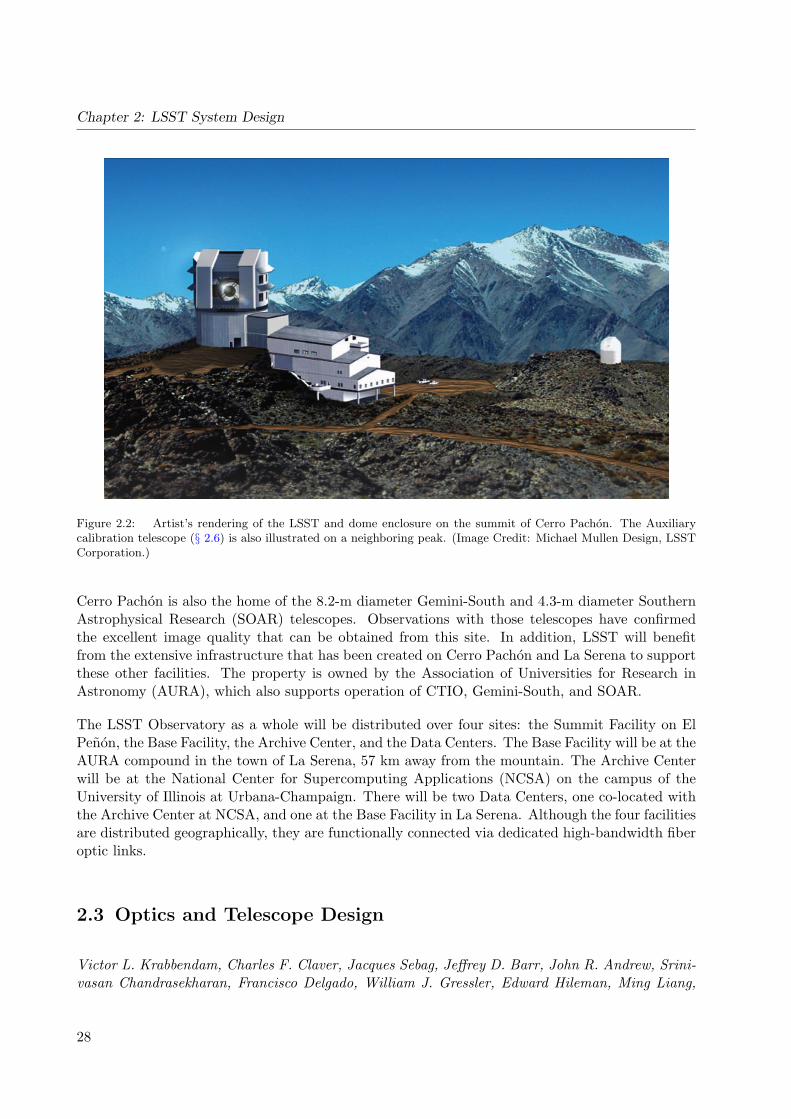
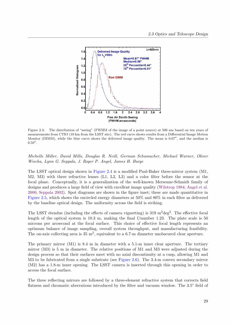
The LSST will be constructed on El Penon Peak (Figure 2.2) of Cerro Pachon in the NorthernChilean Andes. This choice was the result of a formal site selection process following an extensivestudy comparing seeing conditions, cloud cover and other weather patterns, and infrastructureissues at a variety of potential candidate sites around the world. Cerro Pachon is located tenkilometers away from Cerro Tololo Inter-American Observatory (CTIO) for which over ten yearsof detailed weather data have been accumulated. These data show that more than 80% of the nightsare usable, with excellent atmospheric conditions. Differential image motion monitoring (DIMM)measurements made on Cerro Tololo show that the expected mean delivered image quality is 0.67′′

in g (Figure 2.3).

27


Figure 2.2: Artist’s rendering of the LSST and dome enclosure on the summit of Cerro Pachon. The Auxiliarycalibration telescope (§ 2.6) is also illustrated on a neighboring peak. (Image Credit: Michael Mullen Design, LSSTCorporation.)

Cerro Pachon is also the home of the 8.2-m diameter Gemini-South and 4.3-m diameter SouthernAstrophysical Research (SOAR) telescopes. Observations with those telescopes have confirmedthe excellent image quality that can be obtained from this site. In addition, LSST will benefitfrom the extensive infrastructure that has been created on Cerro Pachon and La Serena to supportthese other facilities. The property is owned by the Association of Universities for Research inAstronomy (AURA), which also supports operation of CTIO, Gemini-South, and SOAR.

The LSST Observatory as a whole will be distributed over four sites: the Summit Facility on ElPenon, the Base Facility, the Archive Center, and the Data Centers. The Base Facility will be at theAURA compound in the town of La Serena, 57 km away from the mountain. The Archive Centerwill be at the National Center for Supercomputing Applications (NCSA) on the campus of theUniversity of Illinois at Urbana-Champaign. There will be two Data Centers, one co-located withthe Archive Center at NCSA, and one at the Base Facility in La Serena. Although the four facilitiesare distributed geographically, they are functionally connected via dedicated high-bandwidth fiberoptic links.

2.3 Optics and Telescope Design

Victor L. Krabbendam, Charles F. Claver, Jacques Sebag, Jeffrey D. Barr, John R. Andrew, Srini-vasan Chandrasekharan, Francisco Delgado, William J. Gressler, Edward Hileman, Ming Liang,

28


Figure 2.3: The distribution of “seeing” (FWHM of the image of a point source) at 500 nm based on ten years ofmeasurements from CTIO (10 km from the LSST site). The red curve shows results from a Differential Image MotionMonitor (DIMM), while the blue curve shows the delivered image quality. The mean is 0.67′′, and the median is0.59′′.

Michelle Miller, David Mills, Douglas R. Neill, German Schumacher, Michael Warner, OliverWiecha, Lynn G. Seppala, J. Roger P. Angel, James H. Burge

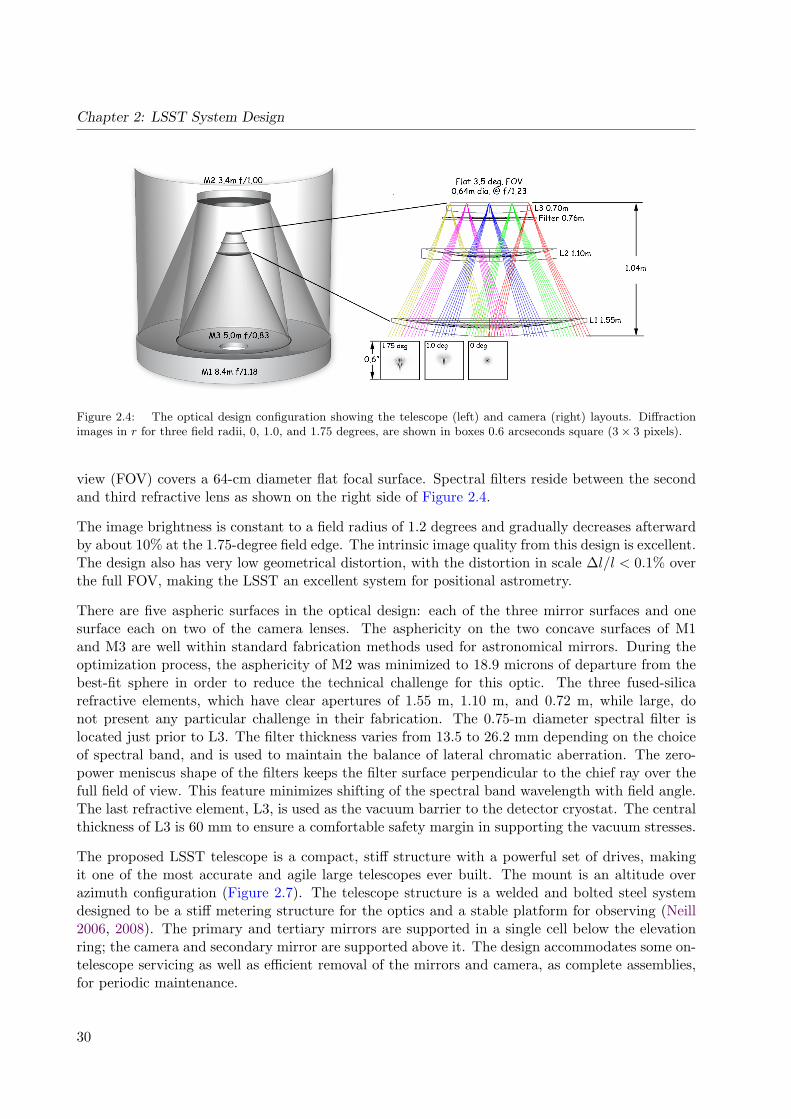
The LSST optical design shown in Figure 2.4 is a modified Paul-Baker three-mirror system (M1,M2, M3) with three refractive lenses (L1, L2, L3) and a color filter before the sensor at thefocal plane. Conceptually, it is a generalization of the well-known Mersenne-Schmidt family ofdesigns and produces a large field of view with excellent image quality (Wilstrop 1984; Angel et al.2000; Seppala 2002). Spot diagrams are shown in the figure inset; these are made quantitative inFigure 2.5, which shows the encircled energy diameters at 50% and 80% in each filter as deliveredby the baseline optical design. The uniformity across the field is striking.

The LSST etendue (including the effects of camera vignetting) is 319 m2deg2. The effective focallength of the optical system is 10.3 m, making the final f/number 1.23. The plate scale is 50microns per arcsecond at the focal surface. This choice of effective focal length represents anoptimum balance of image sampling, overall system throughput, and manufacturing feasibility.The on-axis collecting area is 35 m2, equivalent to a 6.7-m diameter unobscured clear aperture.

The primary mirror (M1) is 8.4 m in diameter with a 5.1-m inner clear aperture. The tertiarymirror (M3) is 5 m in diameter. The relative positions of M1 and M3 were adjusted during thedesign process so that their surfaces meet with no axial discontinuity at a cusp, allowing M1 andM3 to be fabricated from a single substrate (see Figure 2.6). The 3.4-m convex secondary mirror(M2) has a 1.8-m inner opening. The LSST camera is inserted through this opening in order toaccess the focal surface.

The three reflecting mirrors are followed by a three-element refractive system that corrects fieldflatness and chromatic aberrations introduced by the filter and vacuum window. The 3.5◦ field of

29


Figure 2.4: The optical design configuration showing the telescope (left) and camera (right) layouts. Diffractionimages in r for three field radii, 0, 1.0, and 1.75 degrees, are shown in boxes 0.6 arcseconds square (3× 3 pixels).

view (FOV) covers a 64-cm diameter flat focal surface. Spectral filters reside between the secondand third refractive lens as shown on the right side of Figure 2.4.

The image brightness is constant to a field radius of 1.2 degrees and gradually decreases afterwardby about 10% at the 1.75-degree field edge. The intrinsic image quality from this design is excellent.The design also has very low geometrical distortion, with the distortion in scale ∆l/l < 0.1% overthe full FOV, making the LSST an excellent system for positional astrometry.

There are five aspheric surfaces in the optical design: each of the three mirror surfaces and onesurface each on two of the camera lenses. The asphericity on the two concave surfaces of M1and M3 are well within standard fabrication methods used for astronomical mirrors. During theoptimization process, the asphericity of M2 was minimized to 18.9 microns of departure from thebest-fit sphere in order to reduce the technical challenge for this optic. The three fused-silicarefractive elements, which have clear apertures of 1.55 m, 1.10 m, and 0.72 m, while large, donot present any particular challenge in their fabrication. The 0.75-m diameter spectral filter islocated just prior to L3. The filter thickness varies from 13.5 to 26.2 mm depending on the choiceof spectral band, and is used to maintain the balance of lateral chromatic aberration. The zero-power meniscus shape of the filters keeps the filter surface perpendicular to the chief ray over thefull field of view. This feature minimizes shifting of the spectral band wavelength with field angle.The last refractive element, L3, is used as the vacuum barrier to the detector cryostat. The centralthickness of L3 is 60 mm to ensure a comfortable safety margin in supporting the vacuum stresses.

The proposed LSST telescope is a compact, stiff structure with a powerful set of drives, makingit one of the most accurate and agile large telescopes ever built. The mount is an altitude overazimuth configuration (Figure 2.7). The telescope structure is a welded and bolted steel systemdesigned to be a stiff metering structure for the optics and a stable platform for observing (Neill2006, 2008). The primary and tertiary mirrors are supported in a single cell below the elevationring; the camera and secondary mirror are supported above it. The design accommodates some on-telescope servicing as well as efficient removal of the mirrors and camera, as complete assemblies,for periodic maintenance.

30


Figure 2.5: The 50% (plain symbols) and 80% (symbols with lines) encircled energy diameter as a function ofradius in the field of view for the LSST baseline optical design. The image scale is 50 microns per arcsec, or 180 mmper degree.

Figure 2.6: Design and dimensions of the primary and tertiary mirror, showing that the two are built out of asingle mirror blank.

The stiffness of this innovative design is key to achieving a slew and settle time that is beyond thecapability of today’s large telescopes. The size and weight of the systems are a particular challenge,but the fast optical system allows the mount to be short and compact. Finite element analysis hasbeen used to simulate the vibrational modes of the telescope system, including the concrete pier.The frequencies of the four modes with largest amplitudes are (in order):

• 8.3 Hz: Transverse telescope displacement;

• 8.7 Hz: Elevation axis rotation;

• 11.9 Hz: Top end assembly optical axis pumping; and

• 12.6 Hz: Camera pivot.

As described in § 2.1, the standard visit time in a given field is only 34 seconds, quite short for mosttelescopes. The time required to reorient the telescope must also be short to keep the fraction oftime spent in motion below 20% (§ 1.6.2). The motion time for a nominal 3.5◦ elevation move and

31


Figure 2.7: Rendering of the telescope, showing mirror support structures, top end camera assembly, and integratedbaffles.

a 7◦ azimuth move is five seconds. In two seconds, a shaped control profile will move the telescope,which will then settle down to less than 0.1′′ pointing error in three seconds. The stiffness ofthe support structure and drive system has been designed to limit the amplitude and damp outvibrations at these frequencies within this time. The mount uses 400 horsepower in the azimuthdrive system and 50 horsepower in the elevation system. There are four motors per axis configuredin two sets of opposing pairs to eliminate hysteresis in the system. Direct drive systems werejudged overly complicated and too excessive, so the LSST design has each motor working througha multi-stage gear reduction, with power applied through helical gear sets. The 300-ton azimuthassembly and 151-ton elevation assembly are supported on hydrostatic bearings. Each axis usestape encoders with 0.001′′ resolution. Encoder ripple from these tapes often dominates controlsystem noise, so LSST will include adaptive filtering of the signal in the control loop. All-skypointing performance will be better than 2′′. Pointing will directly impact trailing and imagingsystematics for LSST’s wide field of view, so accurate pointing is key to tracking performance.Traditional closed loop guiding will achieve the final level of tracking performance.

2.4 Camera

Kirk Gilmore, Steven M. Kahn, John Geary, Martin Nordby, Paul O’Connor, John Oliver, Scot S.Olivier, Veljko Radeka, Andrew Rasmussen, Terry Schalk, Rafe Schindler, Anthony Tyson, RichardVan Berg

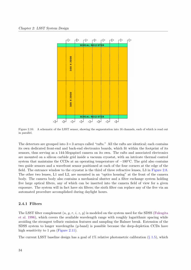
The LSST camera, shown in Figure 2.8, contains a 3.2-gigapixel focal plane array (Figure 2.9)comprised of 189 4 K× 4 K CCD sensors with 10 µm pixels. The focal plane is 0.64 m in diameter,and covers 9.6 deg2 field-of-view with a plate scale of 0.2′′ pixel−1. The CCD sensors are deepdepletion, back-illuminated devices with a highly segmented architecture, 16 channels each, thatenable the entire array to be read out in two seconds (Figure 2.10).

32

2.4 Camera

Figure 2.8: Cutaway drawing of the LSST camera. The camera body is approximately 1.6 m in diameter and 3.5m in length. The optic, L1, is 1.57 m in diameter.

Figure 2.9: With its 189 sensors, each a 4 K × 4 K charge-coupled device (CCD), the focal plane of the cameraimages 9.6 deg2 of the sky per exposure. Note the presence of wavefront sensors, which are fed back to the mirrorsupport/focus system, and the guide sensors, to keep the telescope accurately tracking on a given field.

33


Figure 2.10: A schematic of the LSST sensor, showing the segmentation into 16 channels, each of which is read outin parallel.

The detectors are grouped into 3×3 arrays called “rafts.” All the rafts are identical; each containsits own dedicated front-end and back-end electronics boards, which fit within the footprint of itssensors, thus serving as a 144-Megapixel camera on its own. The rafts and associated electronicsare mounted on a silicon carbide grid inside a vacuum cryostat, with an intricate thermal controlsystem that maintains the CCDs at an operating temperature of −100◦C. The grid also containstwo guide sensors and a wavefront sensor positioned at each of the four corners at the edge of thefield. The entrance window to the cryostat is the third of three refractive lenses, L3 in Figure 2.8.The other two lenses, L1 and L2, are mounted in an “optics housing” at the front of the camerabody. The camera body also contains a mechanical shutter and a filter exchange system holdingfive large optical filters, any of which can be inserted into the camera field of view for a givenexposure. The system will in fact have six filters; the sixth filter can replace any of the five via anautomated procedure accomplished during daylight hours.

2.4.1 Filters

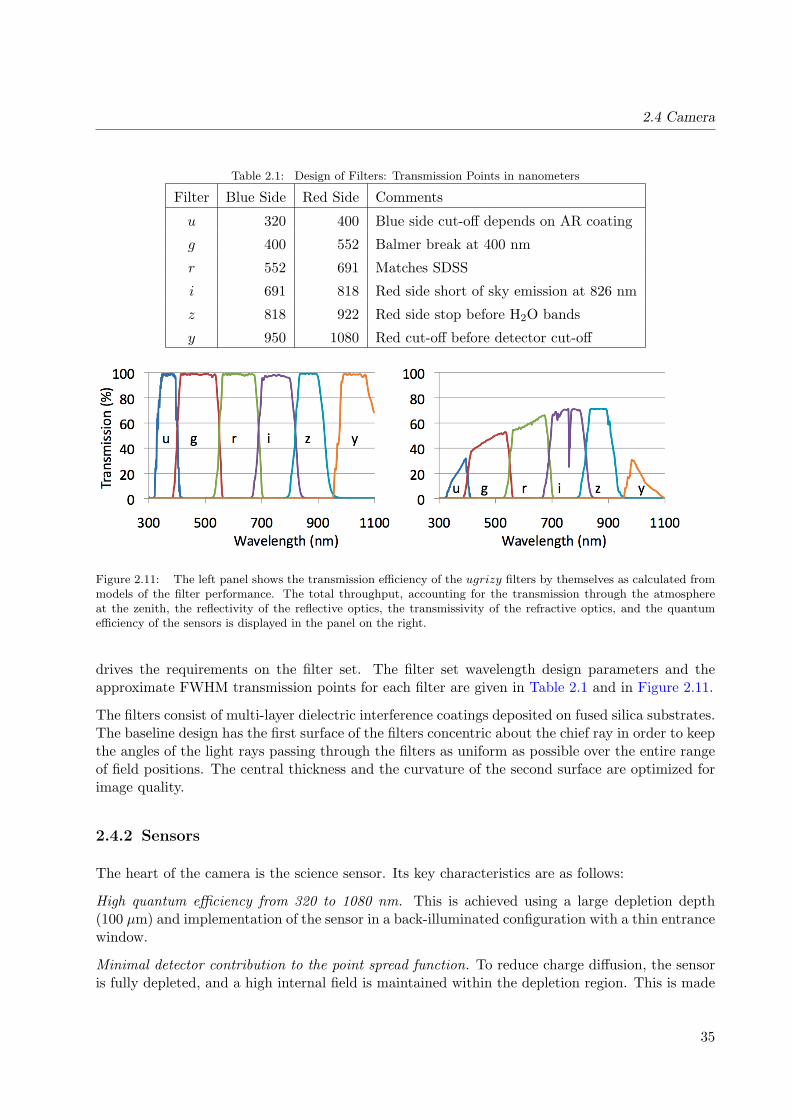
The LSST filter complement (u, g, r, i, z, y) is modeled on the system used for the SDSS (Fukugitaet al. 1996), which covers the available wavelength range with roughly logarithmic spacing whileavoiding the strongest telluric emission features and sampling the Balmer break. Extension of theSDSS system to longer wavelengths (y-band) is possible because the deep-depletion CCDs havehigh sensitivity to 1 µm (Figure 2.11).

The current LSST baseline design has a goal of 1% relative photometric calibration (§ 1.5), which

34

2.4 Camera

Table 2.1: Design of Filters: Transmission Points in nanometers

Filter Blue Side Red Side Comments

u 320 400 Blue side cut-off depends on AR coating

g 400 552 Balmer break at 400 nm

r 552 691 Matches SDSS

i 691 818 Red side short of sky emission at 826 nm

z 818 922 Red side stop before H2O bands

y 950 1080 Red cut-off before detector cut-off

Figure 2.11: The left panel shows the transmission efficiency of the ugrizy filters by themselves as calculated frommodels of the filter performance. The total throughput, accounting for the transmission through the atmosphereat the zenith, the reflectivity of the reflective optics, the transmissivity of the refractive optics, and the quantumefficiency of the sensors is displayed in the panel on the right.

drives the requirements on the filter set. The filter set wavelength design parameters and theapproximate FWHM transmission points for each filter are given in Table 2.1 and in Figure 2.11.

The filters consist of multi-layer dielectric interference coatings deposited on fused silica substrates.The baseline design has the first surface of the filters concentric about the chief ray in order to keepthe angles of the light rays passing through the filters as uniform as possible over the entire rangeof field positions. The central thickness and the curvature of the second surface are optimized forimage quality.

2.4.2 Sensors

The heart of the camera is the science sensor. Its key characteristics are as follows:

High quantum efficiency from 320 to 1080 nm. This is achieved using a large depletion depth(100 µm) and implementation of the sensor in a back-illuminated configuration with a thin entrancewindow.

Minimal detector contribution to the point spread function. To reduce charge diffusion, the sensoris fully depleted, and a high internal field is maintained within the depletion region. This is made

35


possible by the use of high resistivity substrates, high applied voltages, and back-side contacts.Light spreading prior to photo-conversion at longer wavelengths is a minor contributor at the100 µm depletion depth.

Tight flatness tolerances. The fast LSST beam (f/1.23) yields a short depth of field, requiring< 10 µm peak-to-valley focal plane flatness with piston, tip, and tilt adjustable to ∼ 1µm. Thisis achieved through precision alignment and mounting both within the rafts, and within the focalplane grid.

High fill factor. A total of 189 4 K × 4 K sensors are required to cover the 3200 cm2 focal plane.To maintain high throughput, the sensors are mounted in four-side buttable packages and arepositioned in close proximity to one another with gaps of less than a few hundred µm. Theresulting “fill factor,” i.e., the fraction of the focal plane covered by pixels, is 93%.

Fast readout. The camera is read out in two seconds. To reduce the read noise associated withhigher readout speeds, the sensors are highly segmented. The large number of I/O connections thenrequires that the detector electronics be implemented within the cryostat to maintain a manageablenumber of vacuum penetrations.

Our reference sensor design is a CCD with a high degree of segmentation, as illustrated in Fig-ure 2.10. A 4 K × 4 K format was chosen because it is the largest footprint consistent with goodyield. Each amplifier will read out 1,000,000 pixels (a 2000×500 sub-array), allowing a pixel read-out rate of 500 kHz per amplifier. The sensors are mounted on aluminum nitride (AlN) packages.Traces are plated directly to the AlN insulator to route signals from the CCD to the connectorson the back of the package. The AlN package provides a stiff, stable structure that supports thesensor, keeps it flat, and extracts heat via a cooling strap.

2.4.3 Wavefront Sensing and Guiding

Four special purpose rafts, mounted at the corners of the science array, contain wavefront sensorsand guide sensors (Figure 2.9). Wavefront measurements are accomplished using curvature sensing,in which the spatial intensity distribution of stars is measured at equal distances on either sideof focus. Each curvature sensor is composed of two CCD detectors, with one positioned slightlyabove the focal plane, the other positioned slightly below the focal plane. The CCD technology forthe curvature sensors is identical to that used for the science detectors in the focal plane, exceptthat the curvature sensor detectors are half-size so they can be mounted as an in-out defocus pair.Detailed analyses have verified that this configuration can reconstruct the wavefront to the requiredaccuracy. These four corner rafts also hold two guide sensors each. The guide sensors monitor thelocations of bright stars at a frequency of ∼ 10 Hz to provide feedback for a loop that controlsand maintains the tracking of the telescope at an accurate level during an exposure. The baselinesensor for the guider is the Hybrid Visible Silicon hybrid-CMOS detector. We have carried outextensive evaluation to validate that its characteristics (including wide spectral response, high fillfactor, low noise, and wide dynamic range) are consistent with guiding requirements.

36

2.5 Data Management System


Tim S. Axelrod, Jacek Becla, Gregory Dubois-Felsmann, Zeljko Ivezic, R. Lynne Jones, Jeff Kan-tor, R. H. Lupton, David Wittman

The LSST Data Management System (“DMS”) is required to generate a set of data products andto make them available to scientists and the public. To carry out this mission the DMS performsthe following major functions:

• Continually processes the incoming stream of images generated by the camera system duringobserving to produce transient alerts and to archive the raw images.

• Roughly once per year2, creates and archives a Data Release (“DR”), which is a static self-consistent collection of data products generated from all survey data taken from the date ofsurvey initiation to the cutoff date for the Data Release. The data products include optimalmeasurements of the properties (shapes, positions, fluxes, motions) of all objects, includingthose below the single visit sensitivity limit, astrometric and photometric calibration of thefull survey object catalog, and limited classification of objects based on both their staticproperties and time-dependent behavior. Deep coadded images of the full survey area areproduced as well.

• Periodically creates new calibration data products, such as bias frames and flat fields, thatwill be used by the other processing functions.

• Makes all LSST data available publicly through an interface and databases that utilize, tothe maximum possible extent, community-based standards such as those being developedby the Virtual Observatory (“VO”), and facilitates user data analysis and the production ofuser-defined data products at Data Access Centers and at external sites.

The geographical layout of the DMS facilities is shown in Figure 2.12; the facilities include theMountain Summit/Base Facility at Cerro Pachon and La Serena, the central Archive Center atNCSA, the Data Access Centers at NCSA and La Serena, and a System Operations Center. Thedata management system begins at the data acquisition interface between the camera and telescopesubsystems and flows through to the data products accessed by end users. On the way, it movesthrough three types of managed facilities supporting data management, as well as end user sites thatmay conduct science using LSST data or pipeline resources on their own computing infrastructure.

• The data will be transported over existing high-speed optical fiber links from the MountainSummit/Base Facility in Chile to the archive center in the U.S. Data will also flow from theMountain Summit/Base Facility and the archive center to the data access centers over existingfiber optic links. The Mountain Summit/Base Facility is composed of the mountaintoptelescope site, where data acquisition must interface to the other LSST subsystems, and theBase Facility, where rapid-turnaround processing will occur for data quality assessment andnear real-time alerts.

• The Archive Center is a super-computing-class data center with high reliability and avail-ability. This is where the data will undergo complete processing and re-processing andpermanent storage. It is also the main repository feeding the distribution of LSST data tothe community.

2In the first year of operations, we anticipate putting out data releases every few months.

37


Figure 2.12: A schematic map of the LSST DMS facilities. The LSST Telescope Site, located on Cerro Pachon,Chile, is connected to the Base Facility, located in La Serena, Chile by a dedicated fiber link. The Base Facility isconnected to the Archive Center, located at the National Center for Supercomputing Applications in Illinois usingcommercial high-speed network links. The Archive Center, in turn, fans out data to Data Access Centers whichserve the data to clients, and may be located anywhere in the world. The System Operations Center monitors andcontrols the overall operation of the DMS facilities, and provides end-user support facilities.

• Data Access Centers for broad user access are envisioned, according to a tiered access model,where the tiers define the capacity and response available especially to computationally ex-pensive queries and analyses. There are two project-funded Data Access Centers co-locatedwith the Base Facility and the Archive Center. These centers provide replication of all of theLSST data to ensure that disaster recovery is possible. They provide Virtual Observatoryinterfaces to the LSST data products. LSST is encouraging non-US/non-Chilean fundingfor potential partner institutions around the world to host additional Data Access Centers,which could increase end user access bandwidth, provide local high-end computation, andhelp amortize observatory operations costs.

• The System Operations Center provides a control room and large-screen display for super-visory monitoring and control of the DM System. Network and facility status are availableas well as the capability to “drill down” to individual facilities. The Center will also provideDM support to observatory science operations, as well as an end user help desk.

2.5.1 LSST Data Product Overview

Level 1, 2, and 3 Data Products

The data products are organized into three groups, based largely on where and when they areproduced.

38


• Level 1 products are generated by pipeline processing the stream of data from the camerasystem during normal observing. Level 1 data products are, therefore, continuously generatedand/or updated every observing night. This process is of necessity highly automated, andmust proceed with absolutely minimal human interaction. Level 1 products include alerts,i.e., announcements that the flux or position of a given object has changed significantlyrelative to the long-term average. The alerts will be released within 60 seconds of the closingof the shutter at the end of a visit (§ 1.5). In addition to science data products, a numberof Level 1 science data quality assessment (“SDQA”) data products are generated to assessquality and to provide feedback to the Observatory Control System.

• Level 2 products are generated as part of a yearly Data Release. Level 2 products useLevel 1 products as input, and include data products for which extensive computation isrequired (such as variability information, detection, and measurement of the properties offaint objects, and so on), often because they combine information from the stack of manyexposures. Although the steps that generate Level 2 products will be automated, significanthuman interaction may be required at key points to ensure the quality of the data.

• Level 3 data products are derived from Level 1 and/or Level 2 data products to supportparticular science goals, often requiring the combination of LSST data across significant ar-eas on the sky. The DMS will facilitate the creation of Level 3 data products, for exampleby providing suitable Applications Programming Interfaces (APIs) and computing infras-tructure, but is not itself required to create any Level 3 data product. Instead these dataproducts are created externally to the DMS, using software written by, for example, sciencecollaborations. Once created, Level 3 data products may be associated with Level 1 andLevel 2 data products through database federation3. In rare cases, the LSST Project, withthe agreement of the Level 3 creators, may decide to incorporate Level 3 data products intothe DMS production flow, thereby promoting them to Level 2 data products.

Level 1 and Level 2 data products that have passed quality control tests will be accessible tothe public without restriction. Additionally, the source code used to generate them will be madeavailable, and LSST will provide support for building the software system on selected platforms.The access policies for Level 3 data products will be product- and source-specific, and in somecases will be proprietary.

Overview of Pipeline Processing

In the overall organization of the DMS pipelines and productions, “production” has a particularmeaning: it is a coordinated group of pipelines that together carry out a large-scale DMS function.

Alert Production Astronomers interested in transient phenomena of many sorts (Chapter 8)need to know of objects whose flux has changed significantly as soon as possible after the dataare taken. Therefore, the most visible aspect of Level 1 processing is the production of alerts, i.e.,announcements of such variability. The Alert Production is directly fed by the output data streamfrom the camera Science Acquisition System (SDS) during observing. This data stream contains

3See Wikipedia’s article on the subject at http://en.wikipedia.org/wiki/Federated_database.

39

http://en.wikipedia.org/wiki/Federated_database


both unprocessed (raw) camera images, and images that have been corrected for crosstalk by theSDS on the mountain. At the end of a visit, the Alert Production:

• Acquires the raw science images from the camera, and moves them to the Archive Center forpermanent storage.

• Processes the crosstalk-corrected images from the camera to detect transient events within60 seconds of shutter closure for the second exposure in a visit. This will probably be donewith a variant of the Alard & Lupton (1998) image-subtraction algorithm.

• Packages catalog information, together with postage-stamp images of detected transients asalerts and past history of the object, and distributes them to the community as VO events.

• Continuously assesses the data quality of the data stream.

The major steps in the processing flow are:

• Image processing of the raw exposures to remove the instrumental signature, such as bias,flat-field, bad columns, and so on.

• Determination of the World Coordinate System (WCS), image Point-Spread Function (PSF),and rough photometric zeropoint. This produces processed exposures.

• Subtraction of a registered template exposure (a co-addition of previous high-quality imagesof a given field, created in an earlier data release) from the processed exposure, producing adifference exposure.

• Detection of sources (both positive and negative!) in the difference exposure, producing whatwe refer to hereafter as “DIASources.”

• Visit processing logic, which compares the DIASources from the two exposures in the visitto discriminate against cosmic rays, and to flag very rapidly moving Solar System objects.

• “FaintSources,” abbreviated measurements of low signal-to-noise ratio (S/N) detections, areproduced for objects of particular interest, e.g., predicted positions for Solar System objects,or objects that have previously produced alerts.

• Comparison of positive flux DIASources with predictions from the Moving Object Pipeline(MOPS; see § 2.5.3) for already known Solar System objects, as contained in the MovingObject table.

• The Association Pipeline is run to match DIASources to already known astronomical objects,as contained in the Object table.

• DIASources that are detected in both exposures of a visit, and are not matched to a knownSolar System object, produce an alert.

• Quality Assessment is performed at every pipeline stage, stored in database tables, and fedto the Observatory Control System as required.

• The Moving Object Pipeline (§ 2.5.3) is run during the day to interpret each new detectionof a moving object as a new measurement of a Solar System object already in the MovingObject table, or as a previously unknown object, which will be added to the Moving Objecttable. All orbits are refined based on the new measurements from the night.

40


The community has strongly expressed the preference that alerts not be significantly filtered priorto distribution so that science opportunities are not closed off. We have, therefore, adopted verysimple criteria for issuing an alert: 5σ DIASources seen in both exposures of a visit which are notconsistent with cosmic ray events.

Note that no explicit classification of an alert is provided, but users can readily construct classifiersand filters based on information in the Science Database; indeed, this is likely to be part of Level 3software produced by the transient, stellar populations, and supernova science collaborations. Theinformation that could be used for this classification includes the light curve, colors, and shapeinformation for the associated object. Additionally, database queries can readily be formulatedwhich will identify exposures that have generated anomalously large numbers of alerts, presumablydue to image artifacts or processing problems.

As the raw images arrive at the Archive Center, the same processing flow is performed there, withthe consistency of the databases at the Base and Archive Centers being periodically checked. Theduplication of processing is carried out to reduce the data bandwidth required between the Baseand Archive Centers.

Data Release Production At yearly intervals (more often during the first year of the survey)a new Data Release (DR) is produced. A DR includes all data taken by the survey from day oneto the cutoff date for the DR, and is a self-contained set of data products, all produced with thesame pipeline software and processing parameters. The major steps in the processing flow are:

• As in the Alert Production, all raw exposures from the camera are processed to remove theinstrumental signature, and to determine the WCS and PSF, producing processed exposures.This is done with the best available calibration products, which in general will be superiorto those available when the processing was initially done.

• The survey region is tessellated into a set of sky patches of order the size of a CCD, andseveral co-added exposures are produced for each patch from the processed exposures. Theseare a per-band template co-add used for image subtraction; a detection co-add used in theDeep Detection Pipeline (see next item), possibly per-band; and a RGB co-add used forvisualization.

• The Deep Detection Pipeline is run, populating the Object, Source, and FaintSource tables.Rather than working from the co-add, Deep Detection will use the “Multifit” algorithm(§ 2.5.2; Tyson et al. 2008), whereby a model (e.g., a PSF for a stellar object or an exponentialprofile for a disk galaxy) is fit to the entire stack of exposures which contain the object. Thuseach exposure is fit using its own PSF; this results in a set of optimal measurements of theobject attributes over the full time span of the survey, including astrometric parameters suchas proper motion and parallax.

• The Image Subtraction Pipeline is run, as in the Alert Production, yielding DIASources andFaintSources for transient objects.

• The Moving Object Pipeline is run on DIASources, to yield a complete set of orbits for SolarSystem Objects in the Moving Object table.

41


• The Photometric Calibration Pipeline is run on the full set of measurements in the Source,DIASource, and FaintSource catalogs, incorporating measurements from the Auxiliary Tele-scope and other sources of data about the atmosphere to perform a global photometriccalibration of the survey (§ 2.6). In addition to accurate photometry for every measurement,this yields an atmosphere model for every exposure.

2.5.2 Detection and Measurement of Objects

Here we provide more detail on the specific algorithms used to define and measure object propertiesthat are issued with the Data Releases:

Deep Detection Processing

The survey region is organized into overlapping sky patches of order the size of a CCD, and a deepco-added image is created for each patch. The details of the co-add algorithm are still undecided,but the current baseline is to use the Kaiser (2004) algorithm on the full stack of survey imagescontained within the Data Release. The Kaiser algorithm convolves each image with the reflectionof its PSF, and then accumulates with weight inversely proportional to the sky variance. Care willbe taken to ensure that rapidly moving objects, such as Solar System objects, do not appear inthe co-add. An object detection algorithm is then run on the co-add, generating an initial Objectcatalog. An “Object” at this stage is nothing more than a pixel footprint on the sky, possibly withlinks to related Objects in a segmentation tree that has been created by segmenting (deblending)overlapping Objects. The tree will be organized so that the root node is the largest object inthe hierarchy, with the leaf nodes being the smallest. The segmentation/deblending algorithm tobe employed is still under investigation, with Sextractor (Bertin & Arnouts 1996) or the SDSSphotometric pipeline (Stoughton et al. 2002) being examples of the kind of processing involved.The properties of the Objects that are segmented in this way are then determined with Multifitas described below.

Difference Exposure Processing

A new object is created whenever a transient source that is detected in both difference images froma visit does not match any object already in the table. The match will take account of extendednessas well as position on the sky, so that a new point source at the location of a galaxy already in thecatalog (for example, due to a supernova or variable AGN) will result in a new object.

Note that this process cannot be perfect, since measuring the extendedness of objects near thePSF size will always be uncertain. Consequently, there will be cases where flux from a supernovaor AGN point source will be incorrectly added to the underlying galaxy rather than to a new pointsource. Between successive Data Releases, however, these errors will decrease in severity: As thesurvey goes deeper, and accumulates images in better seeing, extendedness will be better measuredby the Multifit procedure, as discussed below.

42


Measuring the Properties of Objects

The image pixels containing an object from all relevant exposures are fit to one or more objectmodels using Multifit, generating model parameters and a covariance matrix. Our choice of modelsis driven by astrophysics, by characteristics of the LSST system, and by computing practicalities.The initial model types are as follows:

Slowly Moving Point Source Model. The Slowly Moving Point Source (SMPS) Model isintended to account for the time varying fluxes and motion on the sky of point sources (usuallystars) with proper motions between zero and roughly 10′′ yr−1. The model accounts for motion withrespect to the local astrometric reference frame that is generated by proper motion, parallax, andpossibly orbital motion with respect to a binary companion. The object properties are measuredin every exposure that contains it. If the S/N in the exposure is above a predetermined threshold,perhaps 5, the measurement generates a row in the Source table. If the S/N is lower than thethreshold, a FaintSource row is generated instead. Lang et al. (2009) have successfully used asimilar modeling and measurement approach to detect very faint brown dwarfs with high propermotion.

The SMPS Model will be fit only to objects that are leaf nodes in the segmentation tree.

Small Object Model. The Small Object (SO) Model is intended to provide a robust parametriza-tion of small (diameter < 1′) galaxy images for weak lensing shear measurement and determinationof photometric redshifts. The definition of the model flux profile is still undecided (Sersic profiles?Superpositions of exponential and de Vaucouleurs profiles?), but should be driven by the needs ofphotometric redshifts (§ 3.8). The measurement of the elliptical shape parameters will be drivenby the needs of weak lensing (Chapter 14).

The SO Model will be fit only to objects that are leaf nodes in the segmentation tree.

Large Object Model. A “large” object is one for which the 20 mag/arcsec2 isophotal diameteris greater than 1′, and less than 80% of the patch size. This includes, for example, the majorityof NGC galaxies. The vast majority of the LSST science will be accomplished with measurementsmade using the SMPS and SO Models, but much valuable science and numerous EPO applicationswill be based on larger objects found in LSST images. To at least partially satisfy this need, largeobjects will have entries in the Object table, but will not have any model fitting performed byMultifit.

Solar System Model. The predicted ephemerides from the orbit for an object in the movingobject table constitutes an object model which is used to measure the object properties in each ex-posure that contains the object. It is not yet decided whether the measurements of faint detectionsshould be at a position entirely fixed by the orbit prediction, or should be allowed to compensatefor prediction error by “peaking up” within some error bound around the prediction.

The Multifit Algorithm

Objects are detected on co-added images, but their models will be fit to the full data set ofexposures on which they appear (n ∼ 400 at the end of the survey in each filter). The motivationfor doing this is two-fold (Tyson et al. 2008). First, the co-add will have a very complicated and

43


discontinuous PSF and depth patchiness due to detector gaps and masked moving objects. Second,although the Kaiser co-add algorithm is a sufficient statistic for the true sky under the assumptionsthat sky noise dominates, and is Gaussian, those assumptions do not strictly hold in real data.

An initial model will be fit to the co-add, to provide a good starting point for the fit to the full dataset. Multifit will then read in all the pixels from the n exposures and perform a maximum likelihoodfit for the model which, when convolved with the n PSFs, best matches the n observations. Thisnaturally incorporates the effects of varying seeing, as the contribution of the better-seeing imagesto the likelihood will be sharper. This approach also facilitates proper accounting for masked areas,cosmic rays, and so on. The best-fit model parameters and their uncertainties will be recorded inan Object table row.

Model Residuals

The measurement process will produce, in conjunction with every source, a residual image thatis the difference of the associated image pixels and the pixels predicted from the model over thefootprint of the model. Characterizing these residuals is important for science such as stronglensing and merging galaxies, that will identify interesting candidates for detailed analysis throughtheir residuals. Selecting the most useful statistical measures of the residuals will be the outcomeof effort during the continuing design and development phase of the project.

2.5.3 The Moving Object Processing System (MOPS)

Identifying moving objects and linking individual detections into orbits, at all distances and solarelongations, would be a daunting task for LSST without advanced software. Each observation fromthe telescope is differenced against a “template” image (built from many previous observations),allowing detection of only transient, variable, or moving objects in the result. These detections arefed into the Moving Object Processing System (MOPS), which attempts to link these individualdetections into orbits.

MOPS uses a three-stage process to find new moving objects (Kubica 2005; Kubica et al. 2005,2007). In the first stage, intra-night associations are proposed by searching for detections forminglinear “tracklets.” By using loose bounds on the linear fit and the maximum rate of motion,many erroneous initial associations can be ruled out. In the current model of operations, LSSTwill revisit observed fields twice each night, with approximately 20–45 minutes between theseobservations. These two detections are what are linked into tracklets. In the second stage, inter-night associations are proposed by searching for sets of tracklets forming a quadratic trajectory.Again, the algorithm can efficiently filter out many incorrect associations while retaining most ofthe true associations. However, the use of a quadratic approximation means that a significantnumber of spurious associations still remains. Current LSST operations simulations (§ 3.1) showthat LSST will image the entire visible night sky approximately every three nights - thus theseinter-night associations of “tracklets” into “tracks” are likely to be separated by 3–4 nights.

In the third stage, initial orbit determination and differential corrections algorithms (Milani et al.2008) are used to further filter out erroneous associations by rejecting associations that do notcorrespond for a valid orbit. Each stage of this strategy thus significantly reduces the number

44

2.6 Photometric Calibration

of false candidate associations that the later and more expensive algorithms need to test. Afterorbit determination has occurred, each orbit is checked against new or previously detected (butunlinked) tracklets, to extend the orbit’s observational arc.

To implement this strategy, the LSST team has developed, in a collaboration with the Pan-STARRSproject (Kaiser et al. 2002), a pipeline based on multiple k-dimensional- (kd-) tree data structures(Kubica et al. 2007; Barnard et al. 2006). These data structures provide an efficient way to indexand search large temporal data sets. Implementing a variable tree search we can link sources thatmove between a pair of observations, merge these tracklets into tracks spread out over tens ofnights, accurately predict where a source will be in subsequent observations, and provide a setof candidate asteroids ordered by the likelihood that they have valid asteroid tracks. Tested onsimulated data, this pipeline recovers 99% of correct tracks for near-Earth and main belt asteroids,and requires less than a day of CPU time to analyze a night’s worth of data. This represents aseveral thousand fold increase in speed over a naıve linear search. It is noteworthy that comparableamounts of CPU time are spent on the kd-tree based linking step (which is very hard to parallelize)and on posterior orbital calculations to weed out false linkages (which can be trivially parallelized).

2.5.4 Long-term Archive of LSST Data

The LSST will archive all observatory-generated data products during its entire 10-year survey. Asingle copy of the resultant data set will be in excess of 85 petabytes. Additional scientific analysesof these data have the potential to generate data sets that significantly exceed this amount.

The longer-term curation plan for the LSST data beyond the survey period is not determined, butit is recognized as a serious concern. This issue is important for all large science archives and itis impractical (perhaps impossible) for individual facilities or researchers to address this problemunilaterally.

The NSF has recognized this issue and has begun soliciting input for addressing long-term curationof scientific data sets via the DataNet and other initiatives. The LSST strongly endorses the needfor this issue to be addressed at the national level, hopefully via a partnership involving government,academic, and industry leaders.


David L. Burke, Tim S. Axelrod, James G. Bartlett, David Cinabro, Charles F. Claver, James S.Frank, J. S. Haggerty, Zeljko Ivezic, R. Lynne Jones, Brian T. Meadows, David Monet, BogdanPopescu, Abhijit Saha, M. Sivertz, J. Allyn Smith, Christopher W. Stubbs, Anthony Tyson

2.6.1 Natural LSST Photometric System

A ground-based telescope with a broad-band detector will observe the integral of the source specificflux density at the top of the Earth’s atmosphere, Fν(λ), weighted by the normalized response

45


function (which includes the effects of the atmosphere and all optical elements), φb(λ),

Fb =∫ ∞

0Fν(λ)φb(λ)dλ, (2.1)

where the index b corresponds to a filter bandpass (b = ugrizy). The chosen units for Fb are Jansky(1 Jansky = 10−26 W Hz−1 m−2 = 10−23 erg cm−2 s−1 Hz−1), and by definition,

∫∞0 φb(λ)dλ = 1.

The corresponding astronomical magnitude is defined as

mb ≡ −2.5 log10

(Fb

FAB

). (2.2)

The flux normalization FAB = 3631 Jy follows the standard of Oke & Gunn (1983).

The normalized response function is defined as

φb(λ) ≡ λ−1Tb(λ)∫∞0 λ−1Tb(λ)dλ

. (2.3)

The λ−1 term reflects the fact that the CCDs used as sensors in the camera are photon-countingdevices rather than calorimeters. Here, Tb(λ) is the system response function,

Tb(λ) = T instrb (λ)× T atm(λ), (2.4)

where T atm is the optical transmittance from the top of the atmosphere to the input pupil of thetelescope, and T instr

b is the instrumental system response (“throughput”) from the input pupil todetector (including filter b). This function is proportional to the probability that a photon startingat the top of the atmosphere will be recorded by the detector. Note that the overall normalizationof both T instr

b and T atm cancels out in Equation 2.3.

An unavoidable feature of ground-based broad-band photometry is that the normalized responsefunction, φb(λ), varies with time and position on the sky and detector due to variations in shapes(spectral profiles) of T atm(λ) and T instr

b (λ). Traditionally, these effects are calibrated out using aset of standard stars. Existing data (e.g., from SDSS) demonstrate that this method is insufficientto deliver the required photometric precision and accuracy in general observing conditions. Instead,the LSST system will measure T atm(λ) and T instr

b (λ) (yielding measured quantities Satm and Sinstrb )

on the relevant wavelength, temporal, and angular scales.

In summary, the basic photometric products will be reported on a natural photometric system,which means that for each photometric measurement, Fmeas

b , a corresponding measured normalizedresponse function, φmeas

b (λ), will also be available. Of course, error estimates for both Fmeasb and

φmeasb (λ) will also be reported. The survey will collect ∼ 1012 such (Fmeas

b ,φmeasb ) pairs over a ten

year period – one pair for each source detection.

2.6.2 Standardized Photometric System

One of the fundamental limitations of broad-band photometry is that measurements of flux, Fmeasb ,

cannot be accurately related to Fν(λ) unless φb(λ) is known. An additional limitation is that Fmeasb

can vary even when Fν(λ) is constant because φb is generally a variable quantity. This variation

46


needs to be accounted for, for example, when searching for low-amplitude stellar variability, orconstruction of precise color-color and color-magnitude diagrams of stars.

Traditionally, this flux variation is calibrated out using atmospheric extinction and color terms,which works for sources with relatively smooth spectral energy distributions. However, strictlyspeaking this effect cannot be calibrated out unless the shape of the source spectral energy distri-bution,

fν(λ) = Fν(λ)/F0, (2.5)

where F0 is an arbitrary normalization constant, is known. If fν(λ) is known, then for a pre-defined “standard” normalized response function, φstd

b (λ) (obtained by appropriate averaging ofan ensemble of φmeas

b during the commissioning period), the measurements expressed on the naturalphotometric system can be “standardized” as

mstdb −mmeas

b ≡ ∆mstd = 2.5 log

(∫∞0 fν(λ)φmeas

b (λ)dλ∫∞0 fν(λ)φstd

b (λ)dλ

), (2.6)

where we have used magnitudes for convenience. While this transformation is in principle exact,mstd

b inherits measurement error in mmeasb , as well as an additional error due to the difference

between the true φb(λ) and the measured φmeasb which will be used in practice. Uncertainties in

our knowledge of fν(λ) will contribute an additional error term to mstdb . Depending on the science

case, users will have a choice of correcting mmeasb using pre-computed ∆mstd for typical spectral

energy distributions (various types of galaxies, stars, and solar system objects, average quasarspectral energy distribution, etc.), or computing their own ∆mstd for their particular choice offν(λ).

2.6.3 Measurement of Instrumental System Response, Ssysb

A monochromatic dome projector system will be used to provide a well-controlled source of lightfor measurement of the relative throughput of the full LSST instrumental system. This includes thereflectivity of the mirrors, transmission of the refractive optics and filters, the quantum efficiencyof the sensors in the camera, and the gain and linearity of the sensor read-out electronics.

An array of projectors mounted in the dome of the LSST enclosure will be illuminated withboth broadband (e.g., quartz lamp) and tunable monochromatic light sources. These “flat-field”projectors are designed to fill the LSST etendue with uniform illumination, and also to limit straylight emitted outside the design acceptance of the system. A set of precision diodes will be used tonormalize the photon flux integrated during flat-field exposures. These photodiodes, together withtheir read-out electronics, will be calibrated at the U.S. National Institute of Standards (NIST) to∼ 0.1% relative accuracy across wavelength from 450 nm to 950 nm. The response of these diodesvaries smoothly across this range of wavelength and provides a well-behaved reference (Stubbs2005). Adjustment of the wavelength of the light source can be as fine as one nanometer, andwill allow precise monitoring of the shape of the bandpasses of the instrumental system during thecourse of the survey (Stubbs & Tonry 2006).

It is anticipated that the shapes of the bandpasses will vary only slowly, so detailed measurementwill need be done only once per month or so. But build-up of dust on the surfaces of the optics

47


will occur more rapidly. The dimensions of these particles are generally large, and their shadowswill be out of focus at the focal plane. So the loss of throughput due to them will be independentof wavelength – i.e., “gray”, and the pixel-to-pixel gradients of their shadows will not be large.Daily broadband and “spot-checks” at selected wavelengths with the monochromatic source willbe used to measure day-to-day changes in the system passbands.

2.6.4 Measurement of Atmospheric Transmittance, Satm

Many studies have shown that atmospheric transmission can be factored into the product of afrequency dependent (“non-gray”) part that varies only on spatial scales larger than the telescopefield-of-view and temporal scales long compared with the interval between LSST exposures; anda frequency independent part (“gray” cloud cover) that varies on moderately short spatial scales(larger than the PSF) and temporal scales that may be shorter than the interval between exposures:

Satm(alt, az, t, λ) = Satmg (alt, az, t)× Satm

ng (alt, az, t, λ). (2.7)

The measurement strategies to determine Satmg and Satm

ng are quite different:

• Satmng is determined from repeated spectroscopic measurements of a small set of probe stars

by a dedicated auxiliary telescope.

• Satmg is determined from the LSST science images themselves, first approximately as each

image is processed, and later more precisely as part of a global photometric self-calibrationof the survey. The precise measurement of Satm

g is based on the measured fluxes of a verylarge set of reference stars that cover the survey area and are observed over many epochs.Every exposure contains a large enough set of sufficiently stable stars that a spatial map canbe made of Satm

g across each image.

The LSST design includes a 1.2-m auxiliary calibration telescope located on Cerro Pachon nearthe LSST that will be used to measure Satm

ng (alt, az, t, λ). The strategy is to measure the fullspatial and temporal variation in atmospheric extinction throughout each night independently ofoperations of the main survey telescope. This will be done by repeatedly taking spectra of a smallset of probe stars as they traverse the sky each night. These stars are spaced across the sky tofully cover the area surveyed by the LSST main telescope. The calibration will use state-of-the-artatmospheric models (Stubbs et al. 2007) and readily available codes (MODTRAN4) to accuratelycompute the signatures of all significant atmospheric components in these spectra. This will allowthe atmospheric mix present along any line of sight at any time to be interpolated from themeasured data. The probe stars will be observed many times during the LSST survey, so the SEDof each star can be bootstrapped from the data. The instrumental response of the spectrographcan also be bootstrapped from the data by including stars with a variety of SEDs over a broadrange of airmass.

2.6.5 Calibration Procedure

Two levels of LSST calibration will be carried out at differing cadences and with differing per-formance targets. A nightly data calibration based on the best available set of prior calibrated

48


observations will provide “best-effort” precision and accuracy. This calibration will be used forquality assurance, generation of alerts to transients, and other quantities appropriate for Level 1Data Products (§ 2.5.1). A more complete analysis will recalibrate the data accumulated by thesurvey at periodic “Data Release” dates (Level 2 in the terminology of § 2.5.1). It is this repeatedcalibration of the accumulated survey that will be held to the survey requirements for photometricrepeatability, uniformity, and accuracy.

LSST photometric calibration is then separated into three parts that address different sciencerequirement specifications:

• Relative calibration: normalization of internal (instrumental) measurements in a given band-pass relative to all other measurements made in the same bandpass across the sky.

• Absolute calibration of colors: determination of the five unique differences between fluxnormalizations of the six bands (color zero points).

• Absolute calibration of flux: definition of the overall physical scale of the LSST magnitudesystem, i.e., normalization to FAB in Equation 2.2.

Relative Calibration

Precision relative calibration of LSST photometry will be accomplished by analysis of the repeatedobservations of order 108 selected bright (17 < r < 20) isolated stars during science operationsof the survey. The LSST image processing pipelines will extract raw ADU counts for these starsfrom each image, and the data release Calibration Pipeline will process data from the calibra-tion auxiliary subsystems to determine the optical bandpass appropriate for each image. Thesemeasurements will be used to determine calibrations for all sources detected on each image.

After reduction of each image in the accumulated survey, the Calibration Pipeline will executea global self-calibration procedure that will seek to minimize the dispersion of the errors in allobservations of all reference stars. This process is based on techniques used in previous imagingsurveys (Glazebrook et al. 1994; MacDonald et al. 2004), and the specific implementation usedby LSST will be based on the “Ubercal” procedure developed for SDSS (Padmanabhan et al.2008). “Calibration patches” of order the size of a single CCD will be defined on the camera focalplane. The LSST survey will dither pointings from epoch to epoch to control systematic errors,so stars will fall on different patches on different epochs across the sky. The measured magnitudesof reference stars will be transformed (Equation 2.6) to the LSST standard bandpass using theaccumulated estimates of the colors of each star and the corresponding measured observationalbandpasses. The Calibration Pipeline will minimize the relative error δb(p, j) in the photometriczero-point for each patch, p, on each image, j, of the accumulated survey by minimizing,

χ2 =∑(i,j)

(mstd,meas

b (i, j)−(mstd,true

b (i) + δb(p, j)))2

(δmstd,meas

b (i, j))2 , (2.8)

where the magnitudes are in the standard system, and the summation is over all stars, i, in allimages, j. These δb(p, j) will be used to correct the photometry for all other sources in patch, p,on image, j.

49


Absolute Calibration of Colors and Flux

There are six numbers, ∆b, for the entire survey that set the zeropoints of the standard bandpassesfor the six filters. These six numbers can be expressed in terms of a single fiducial band, which wetake to be the r band,

∆b = ∆r + ∆br. (2.9)

The LSST strategy to measure the observational bandpass for each source is designed to reduceerrors, ∆br, in the five color zero points, to meet specifications in the survey requirements. Thisprocess will be validated with the measured flux from one or more celestial sources, most likelyhot white dwarfs whose simple atmospheres are reasonably well-understood.

At least one external flux standard will be required to determine ∆r (one number for the wholesurvey!). While one celestial standard would be formally sufficient, choosing a number of such stan-dards would provide a powerful test for ∆r. Identification of such a standard, or set of standards,has not yet been done.

2.7 Astrometric Calibration

David Monet, David L. Burke, Tim S. Axelrod, R. Lynne Jones, Zeljko Ivezic

The astrometric calibration of LSST data is critical for many aspects of LSST operations (pointing,assessment of camera stability, etc.) and scientific results ranging from the measurement of stellarparallaxes and proper motions to proper performance of difference image analysis.

The core of the astrometric algorithm is the simultaneous solution for two types of unknowns, thecoefficients that transform the coordinates on the focal plane measured in a given exposure intosome common coordinate system (absolute astrometry), and the positions and motions of eachstar (relative astrometry). Whereas a direct solution exists, it involves the inversion of relativelylarge matrices and is rarely used. Instead, the solution is based on an iterative improvement giventhe prior knowledge of positions of a relatively small number of stars (from a reference catalogor similar). All observations for all stars in a small area of sky are extracted from the database.Using the catalog positions for the stars as a first guess, the transformations from each observationto the catalog system are computed, and then all measures for each star are used to compute thenew values for position and motion.

2.7.1 Absolute Astrometry

The current realization of the International Celestial References Frame (ICRF) is defined by thestars in ESA’s Hipparcos mission catalog. ESA’s Gaia mission, set to launch in 2012, will improvethe ICRS and ICRF by another two orders of magnitude down to the level of a few micro-arcseconds.

Absolute calibration consists of computing the positions of all the detected sources and objects inthe LSST imaging with respect to the ICRF. Were no improved catalogs available between nowand LSST commissioning, the reference catalogs would be the US Naval Observatory’s UCAC-3catalog for bright optical stars (down to about 16th magnitude, uncomfortably close to LSST’s

50

2.7 Astrometric Calibration

saturation limit) or the NASA 2MASS catalog whose near-IR positions for optical stars have anaccuracy of 70-100 milli-arcseconds (mas) for individual stars and systematic errors in the range of10-20 mas. There are large numbers of 2MASS stars in each and every LSST field of view, so theastrometric calibration is little more than the computation of a polynomial that maps position onthe focal plane into the system of right ascension and declination defined by the measured positionsof catalog objects. The transformation is encapsulated in the World Coordinate System (WCS)keywords in the Flexible Image Transport System (FITS) header for each image.

One of the key astrometric challenges in generating and using these WCS solutions is the distinctionbetween “observed” and “catalog” coordinates. When LSST takes an image, the stars and galaxiesare at their observed positions. These positions include the astrometric effects of proper motion,parallax, differential refraction, differential aberration, and others. Most applications work incatalog coordinates such as the J2000 positions for objects or the equivalent for image manipulation.The astrometric calibration will provide a rigorous method for going between these coordinatesystems.

2.7.2 Differential Astrometry

Differential astrometry is for most science the more important job to be done. The differentialsolution, which provides measures for the stellar parallax, proper motion, and perturbations (e.g.,due to binary companions), can be substantially more accurate than the knowledge of the absolutecoordinates of an object. The task is to measure centroids on images and to compute the trans-formation from the current frame into the mean coordinate system of other LSST data, such asthe deep image stacks or the different images from the multi-epoch data set. The photon noiselimit in determining the position of the centroiding of a star is roughly half the FWHM of theseeing disk, divided by the signal-to-noise ratio of the detection of the star. The expectation isthat atmospheric seeing will be the dominant source of astrometric error for sources not dominatedby photon statistics. Experiments with wide-field imaging on the Subaru Telescope (§ 3.6) suggestthat accuracy will be better than 10 mas per exposure in the baseline LSST cadence, although itmay be worse with objects with unusual SEDs such that simple differential color refraction analysisfails, or for exposures taken at extreme zenith angles.

Perhaps the biggest unknown in discussion of differential astrometry is the size of the “patch” onthe sky over which the astrometric solution is taken. If the patch is small enough, the astrometricimpact of the unaveraged turbulence can be mapped with a simple polynomial, and the differentialastrometric accuracy approaches that set by the photon statistics. Our current understanding ofatmospheric turbulence suggests that we will be able to work with patches between a few and 10arcmin in size, small enough that the geometry can fit with low-order spatial polynomials. Thecurrent approach is to use the JPL HEALPix tessellation strategy. For each solution HEALPix(el),separate spatial transformations are computed for each CCD of each observation. These producemeasures for each object in a mean coordinate system, and these measures can be fit for position,proper motion, parallax, refraction, perturbations from unseen companions, and other astrometricsignals. Given the very faint limiting magnitude of LSST, there should be be a sufficient numberof astrometrically useful galaxies to deliver a reasonable zero-point within each HEALpix4. The

4Quasars will be less useful; they are less numerous, and their very different SEDs cause different refraction fromstars.

51

Chapter 2: References

characterization of the zero-point errors and the astrometric utility of galaxies will be the majorwork area for the astrometric calibration team.

References

Alard, C., & Lupton, R. H., 1998, ApJ , 503, 325Angel, R., Lesser, M., Sarlot, R., & Dunham, E., 2000, Astronomical Society of the Pacific Conference Series, Vol.

195, Design for an 8-m Telescope with a 3 Degree Field at f/1.25: The Dark Matter Telescope, W. van Breugel &J. Bland-Hawthorn, eds. p. 81

Barnard, K. et al., 2006, Society of Photo-Optical Instrumentation Engineers (SPIE) Conference, Vol. 6270, TheLSST moving object processing pipeline

Bertin, E., & Arnouts, S., 1996, A&AS , 117, 393Fukugita, M., Ichikawa, T., Gunn, J. E., Doi, M., Shimasaku, K., & Schneider, D. P., 1996, AJ , 111, 1748Glazebrook, K., Peacock, J. A., Collins, C. A., & Miller, L., 1994, MNRAS , 266, 65Kaiser, N., 2004, Unpublished Pan-STARRS Document PSDC-002-011Kaiser, N. et al., 2002, Society of Photo-Optical Instrumentation Engineers (SPIE) Conference, Vol. 4836, Pan-

STARRS: A Large Synoptic Survey Telescope Array, J. A. Tyson & S. Wolff, eds. pp. 154–164Kubica, J., 2005, PhD thesis, Carnegie Mellon University, United States – PennsylvaniaKubica, J. et al., 2005, Bulletin of the American Astronomical Society, Vol. 37, Efficiently Tracking Moving Sources

in the LSST. p. 1207—, 2007, Icarus, 189, 151Lang, D., Hogg, D. W., Jester, S., & Rix, H.-W., 2009, AJ , 137, 4400MacDonald, E. C. et al., 2004, MNRAS , 352, 1255Milani, A., Gronchi, G. F., Farnocchia, D., Knezevic, Z., Jedicke, R., Denneau, L., & Pierfederici, F., 2008, Icarus,

195, 474Neill, D. R., 2006, Society of Photo-Optical Instrumentation Engineers (SPIE) Conference Series, Vol. 6267, LSST

telescope mount concept—, 2008, LSST Telescope Pier. LSST Docushare Document-3347Oke, J. B., & Gunn, J. E., 1983, ApJ , 266, 713Padmanabhan, N. et al., 2008, ApJ , 674, 1217Seppala, L. G., 2002, Society of Photo-Optical Instrumentation Engineers (SPIE) Conference Series, Vol. 4836,

Improved optical design for the Large Synoptic Survey Telescope (LSST), J. A. Tyson & S. Wolff, eds. pp.111–118

Stoughton, C. et al., 2002, AJ , 123, 485Stubbs, C. W., 2005, An Overview of the Large Synoptic Survey Telescope (LSST) System, Presentation 180.02 at

the 205th Annual Meeting of the American Astronomical SocietyStubbs, C. W. et al., 2007, PASP , 119, 1163Stubbs, C. W., & Tonry, J. L., 2006, ApJ , 646, 1436Tyson, J. A., Roat, C., Bosch, J., & Wittman, D., 2008, in Astronomical Society of the Pacific Conference Series,

Vol. 394, Astronomical Data Analysis Software and Systems XVII, R. W. Argyle, P. S. Bunclark, & J. R. Lewis,eds., p. 107

Wilstrop, R. V., 1984, MNRAS , 210, 597

52

2 lsst system design - welcome | the large … · 2 lsst system design john r ... space of possible...

Documents