§2 – diffraction methods and structure determination

$: §2 – Diffraction methods and structure determination$
§2 – Diffraction methods and structure determination :

§2 – Diffraction methods and structure determination

2.1 Lattice Planes

We can use the Miller index system to identify planes within a lattice.

We will consider a 2-dimensional system because it is easier to visualise, but the Miller index system is usually applied in 3 dimensions.

The intercepts of the plane with the lattice axes are denoted m1, m2, m3.

We then take the reciprocal of these lengths.

The Miller indices are then the smallest integers with the same ratio. We usually write the Miller indices in parentheses as h k l .

Taking the example shown in Fig. (2.1):

Intercepts

m1=2 ; m2=2 ; m3=∞

Reciprocals

1m1=1

2; 1m2=1

2; 1m3=0

Miller Indices

Multiplying by 2 gives:

– 1 –Last Modified: 05/11/2006

Figure 2.1: Diagram of lattice points with intersecting plane (drawn in red). The lengths m1 and m2 are

measured in units of primitive translational vectors.

a1

a2

m1

m2


h k l =1 1 0

If the plane cuts an axis on the negative side of the origin, the corresponding index is negative. This is usually denoted by an overbar.

We denote sets of symmetry-equivalent planes by braces (curly brackets) around the indices.

Example

The set of cube faces is {1 0 0}=1 0 0 , 0 1 0 , 0 0 1 , 1 0 0 , 0 1 0 , 0 0 1 .

The indices [u v w] are used to denote the smallest integers that have the ratio of the components of a vector in the desired direction.

For example, the a1 axis is the [1 0 0] direction, the line a1=−a2 ; a3=0 ; a10 is the[1 1 0] .

2.2 Bragg's Law

In 1915, W. L. Bragg presented a simple explanation of the interference effects seen in X-ray diffraction from a crystal. It can also be used to describe electron and neutron diffraction interference patterns.

Suppose that the incident waves are reflected specularly (like a mirror) from parallel planes of atoms in the crystal, where each plane reflects just a small fraction of the radiation. Then, the angle of incidence equals the angle of reflection.

Diffracted beams are detected when the reflected beams interfere constructively.

Assume elastic scattering (no energy change after reflection).

If the lattice planes are a distance d apart, the path difference for rays reflected by adjacent planes is2 d sin , where θ is the angle from the plane.

Constructive interference occurs when the path difference is an integer number of wavelengthsn , giving the well-known Bragg law:

(2.1)

Equation (2.1) shows that Bragg reflection can only occur for light at a wavelength ≤2d and since d≃A , this explains why we cannot use visible light to produce such effects.

This simple picture of interference can take us a long way.


2 d sin=n


The plane separation can be found directly from the lattice, so we can determine exactly what angles Bragg will diffract X-rays.

Most angles do not correspond to a planar spacing, so there are only a few sharp peaks in the diffraction pattern.

2.3 Reciprocal Lattice Vectors

If the electron number density n r in a crystal is a periodic function of r with periodsa1. a2 a3 in the directions of the cell axes, then the number density satisfies:

(2.2)

Using Fourier analysis, we can show that such a periodic function in three-dimensions can be written in terms of a set of vectors G :

(2.3)

These new vectors must be invariant under all T that leave the crystal invariant.

Inverting the Fourier series, integrating over the volume of a cell gives:

(2.4)


n rT =n r

n r =∑GnG exp i G⋅r

Figure 2.2: Geometrical representation of Bragg reflection from a plane of atoms. Here, d is the spacing of parallel atomic planes. The difference in phase of waves after

reflection from successive planes is 2πn.

nG=V cell−1∫

V cell

d V nr exp i G⋅r


If we set rrT into equation (2.3), we get an extra factor exp i G⋅T .

In order to satisfy equation (2.2), we require that:

(2.5)

Where: n∈ℤ (n is an integer).

Assume we can write:

(2.6)

Where vi can be any integers.

We want to construct a set of vectors such that:

(2.7)

(The factor of 2π is not strictly necessary as it can be absorbed into the coefficients, and is omitted by crystallographers. However, we choose to retain it in Solid State Physics).

If bi∝ a j× ak ,where i≠ j≠k , then:

bi⋅a j∝a j⋅ a j× ak =0 as required.

And:

bi⋅a i∝ai⋅ a j× ak =V cell

Thus, it is clear to see that the vectors bi must take the form:

(2.8)

The vector G is called the reciprocal lattice vector and the vectors bi are the primitive vectors of the reciprocal lattice.


G=v1b1v 2

b2v3b3

G⋅T=2n

bi⋅a j=2ij

b1=2 a2× a3

V cell; b2=2 a3× a1

V cell; b3=2 a1×a2

V cell


Every crystal structure has a crystal lattice and a reciprocal lattice. The diffraction pattern of a crystal gives a map of the reciprocal lattice and not the crystal lattice.

Vectors in a reciprocal lattice have units [L]-1, hence the term reciprocal.

A reciprocal lattice can be seen as a lattice in the Fourier space or reciprocal space associated with the crystal.

We can check that bi do indeed have the correct form by checking that equation (2.3) satisfies (2.2):

n rT =∑G

n Gexpi G⋅r exp i G⋅T

G⋅T=v1b1v2

b2v3b3⋅u1 a1u2 a2u3 a3

G⋅T=2v1u1v2u2v3u3

But, u i , v i are all integers, so all the terms in the bracket must also be an integer. Thus:

exp i G⋅T =exp [2 n i ]=1

2.4 Laue Method

A travelling electromagnetic wave can be described by the wavefunction:

(2.9)

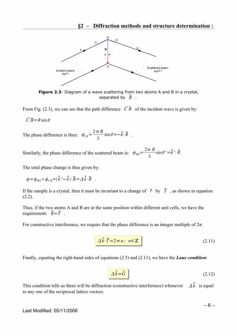
If A and B in Figure 2.3 are identical atoms, then the phase difference between waves scattered by each of them will be the same.

If A' is the amplitude of the scattered beam, then the scattered wave has wavefunction:

(2.10)

We will assume elastic scattering:

⇒ ∣k∣=∣k '∣=2


r =Ae ik⋅r

' r =A' e i k '⋅r


From Fig. (2.3), we can see that the path difference C B of the incident wave is given by:

C B=R sin

The phase difference is then: CB=2R

sin=−k⋅R .

Similarly, the phase difference of the scattered beam is: BD=2 R

sin '=k '⋅R

The total phase change is thus given by:

=BDCB=k '−k ⋅R=k⋅R .

If the sample is a crystal, then it must be invariant to a change of r by T , as shown in equation (2.2).

Thus, if the two atoms A and B are at the same position within different unit cells, we have the requirement: R=T .

For constructive interference, we require that the phase difference is an integer multiple of 2π:

(2.11)

Finally, equating the right-hand sides of equations (2.5) and (2.11), we have the Laue condition:

(2.12)

This condition tells us there will be diffraction (constructive interference) whenever k is equal to any one of the reciprocal lattice vectors.


Figure 2.3: Diagram of a wave scattering from two atoms A and B in a crystal, separated by R .

k⋅T=2n; n∈ℤ

k=G

A

B

CD

Incident beam:Aei(k.r)

Scattered beam:A'ei(k'.r)

k k'

θ

R

θ'


This shows us that diffraction occurs only at a set of discrete points.

We note that equation (2.12) is a vector equation, so all three components must be satisfied separately. Using the orthogonality condition in equation (2.7) gives the three Laue equations, which must all be satisfied for a given k . This is just a restatement of equation (2.11).

(2.13)

2.5 Equivalence of Bragg and Laue Explanations

The points of the reciprocal lattices are normal to the planes.

In section 2.1, we defined the Miller indices h k l . These are equivalent to the integersv1 v2 v3 in the reciprocal lattice vector G .

The vector G=h b1k b2 l b3 points in a direction normal to the plane [hk l ] .

The length of this vector is2d , where d is the Bragg spacing.

Since, ∣k∣=∣k '∣ , the vector k must point in the specular direction, as shown in Fig. 2.4 below:

The geometry of Fig. 2.4 shows us that:

∣k∣=∣G∣=2∣k∣sin=2d


a1⋅k=2v1 ; a2⋅k=2 v2 ; a3⋅k=2v3

Figure 2.4: Schematic of Bragg diffraction. Δk is perpendicular (specular) to the Bragg plane at the

scattering point.

θ

k k'

Δk


Since ∣k∣=2

, we have:

2 d sin= , which is Bragg's law for constructive interference, where n = 1.

2.6 Examples of Reciprocal Lattices

a) 2D Rectangular Lattice

Let a3 point into the paper. Thus, the crystal lattice is:

From Fig. 2.5, the reciprocal lattice vectors are:

b1=2a2a3

a1a2a3x=

2a1x ; b2=2

a3a1

a1a2a3y=

2a2y

Thus, the reciprocal lattice is:

The axis lengths in reciprocal space are in units [L]-1 and the longer direction in real space becomes the shorter in reciprocal space and vice versa.

Note:

In the special case of the square lattice, the reciprocal lattice remains square.


Figure 2.5: Crystal lattice of 2-dimensional rectangular structure

Figure 2.6: Reciprocal lattice of a 2-dimensional rectangular structure

a1=a1 xx

a2=a2 y

x b1=2a1x

b2=2a2

y


b) 2D Hexagonal Lattice

Again, let a3 point into the paper.

In this case the real lattice has the form: a1=a2=a ; a1⋅a2=32

a1a2=32a2≠a1a2 .

V cell=32

a1a2a3

∣b1∣=∣b2∣=23

2a

Generally, the directions of the vectors bi are perpendicular to the vectors a i with length

proportional to2ai

.

c) FCC Lattice

The primitive lattice vectors of an fcc crystal have a more complicated relationship than either of the above examples.

We can show that the reciprocal lattice of an fcc crystal is a bcc lattice.


Figure 2.7: Crystal lattice of 2-dimensional hexagonal structure.

Figure 2.8: Reciprocal lattice of a 2D hexagonal structure.

x a1

a2

120°

x

60°

b1

b2


Also, the reciprocal lattice of a bcc crystal is an fcc lattice.Note:

The reciprocal of a reciprocal lattice is always the original lattice.

The volume of a reciprocal lattice cell is23

V cell, where: V cell is the volume of the original

lattice.

2.7 Diffraction from SC Lattice

a) Reciprocal View of Problem

A simple cubic lattice has a single real space lattice parameter a0 .

The reciprocal lattice, is also a simple cubic lattice, with spacing b0=2a0

.

The reciprocal lattice vector for a SC structure is given by: G=2a0

h xk yl z .

Remember, the Laue condition for diffraction is: k=G .

So, the allowed values of k are: ∣k∣=2a0 h2k 2l 2 .

Also, ∣k∣=2k sin , where: 2θ = Bragg angle.

A powder sample (common case) has random orientation.

Plotting intensity against Bragg angle shows a series of peaks.

– 10 –Last Modified: 05/11/2006

Figure 2.9: Example of a reciprocal lattice vector in a SC crystal. Values in parentheses indicate

Miller indices.

b0 2 b0 3 b0

b0

2 b0

3 b0

(1 0 0)

(1 1 0) (2 1 0)


Overview of analysis procedure

1. Read off values of 2 : the Bragg angle;

2. Convert these angles to a list of values of ∣k∣2= 2a0

2

h2k 2l 2 ;

3. Divide by the smallest k 2 value to factor out a0 ;

4. Look for simple fractions.

Note:

Not all peaks will appear. There may also be degenerate cases. This can be seen below:

(h k l) h2 + k2 + l2

(1 0 0) 1

(1 1 0) 2

(1 1 1) 3

(2 0 0) 4

(2 1 0) 5

(2 1 1) 6

(2 2 0) 8

(2 2 1) 9

(3 0 0) 9

As we will see later, the peak spacings become rapidly more complicated.

– 11 –Last Modified: 05/11/2006

→ No peak at 7

}degenerate


b) Real-space View of Problem

2 d sin=

⇒ d= 2sin

Analysis Procedure

1. Read off values of 2 : the Bragg angle;

2. Convert these angles to a list of values of1d 2=

1a0

2 h2k 2l 2 ;

3. Divide by the smallest1d 2 value to factor out a0 ;

As can be seen, the method is the same for the real-space and reciprocal-space views: in the SC case, both are equally difficult to calculate.

The problem is that the “spacing formula” is non-trivial for more complicated lattices than the SC structure.

2.8 Lattices with a Basis

So far, we have only considered cases where R=T when we considered diffraction.

All points that are related by lattice vectors T will be in phase whenever k=G , so they will interfere constructively.

For points in the basis, within the unit cell there will be a phase shift. Thus the interference pattern will be more complicated, even when k=G .

– 12 –Last Modified: 05/11/2006

Figure 2.10: Example of a real-space lattice in a SC crystal.

d=a0/h2k 2l 2

a1

a2

(h k l) planes


If we keep the k=G condition, we only need to consider one unit cell.

For the general case, equation (2.11) still holds: k⋅T=2n .

But, we will now introduce a variable phase factor for point r in the unit cell: k⋅r≠2n .

The amplitude of the interference pattern will be of the form:

A=∑rWeight r exp i G⋅r . summing over points of the unit cell.

But, since the X-rays are scattered by electrons, the weight is proportional to the electron number density n r .

This Fourier series becomes an integral:

(2.14)

This is the structure factor, and is equivalent to equation (2.4) multiplied by the volume of the unit cell.

Note:

If k≠G , then Ak =0 .

Thus, n r is entirely described by the (generally infinite) set of discrete complex numbers, SG

.The important thing to note is that the measured peak intensities of Bragg diffraction are the squares of the amplitudes of the structure factors.

2.9 “Structure Factor” of an Atom

We can write the structure factor of a free atom as:

(2.15)

Crucial to this approach, most of the density of a free atom remains unchanged when it is bound in a crystal.

Thus, the functions fG can be determined from theory.

Atoms are (to a good approximation) spherically symmetric, so are f G . Also, to a first

– 13 –Last Modified: 05/11/2006

SG=∫V cell

n r expi G⋅r d r

f G=∫ natom r exp i G⋅r d 3r


approximation, we can assume that atoms are point-like.

This means that f G are approximately converge on a single value (for a given atom) .

In fact, f G≃Z≡atomic number .

2.10 Structure Factor of a Multi-Atom Basis

Again, assume that the atoms are point-like. This means we have a set of discrete values f j .

Thus, the structure factor integral in equation (2.15) becomes a summation:

(2.16)

Where r j∈unit cell is the position of the j'th atom.

The relative phases of the different points in the unit cell can often lead to cancellations, so some values of the structure factors will be zero.

We can identify different types of lattices using selection rules.

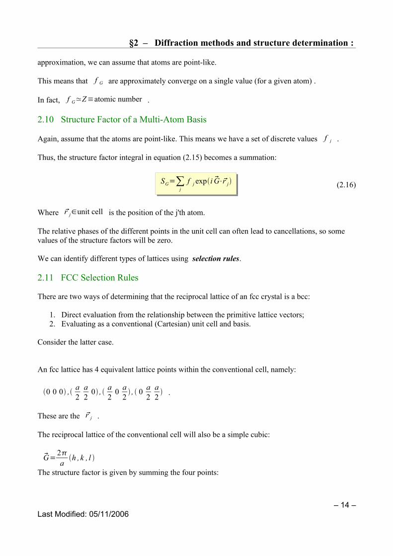
2.11 FCC Selection Rules

There are two ways of determining that the reciprocal lattice of an fcc crystal is a bcc:

1. Direct evaluation from the relationship between the primitive lattice vectors;2. Evaluating as a conventional (Cartesian) unit cell and basis.

Consider the latter case.

An fcc lattice has 4 equivalent lattice points within the conventional cell, namely:

0 0 0 , a2

a2

0 , a2

0 a2 , 0 a

2a2 .

These are the r j .

The reciprocal lattice of the conventional cell will also be a simple cubic:

G=2ah , k , l

The structure factor is given by summing the four points:

– 14 –Last Modified: 05/11/2006

SG=∑jf j expi G⋅r j


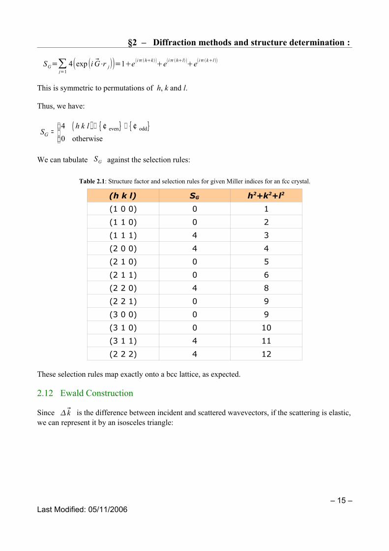
SG=∑j=1

4exp i G⋅r j=1e ihk eihl eikl

This is symmetric to permutations of h, k and l.

Thus, we have:

( ) { } { }even odd40 otherwiseG

h k lS

∈ ∨=

¢ ¢

We can tabulate SG against the selection rules:

Table 2.1: Structure factor and selection rules for given Miller indices for an fcc crystal.

(h k l) SG h2+k2+l2

(1 0 0) 0 1

(1 1 0) 0 2

(1 1 1) 4 3

(2 0 0) 4 4

(2 1 0) 0 5

(2 1 1) 0 6

(2 2 0) 4 8

(2 2 1) 0 9

(3 0 0) 0 9

(3 1 0) 0 10

(3 1 1) 4 11

(2 2 2) 4 12

These selection rules map exactly onto a bcc lattice, as expected.

2.12 Ewald Construction

Since k is the difference between incident and scattered wavevectors, if the scattering is elastic, we can represent it by an isosceles triangle:

– 15 –Last Modified: 05/11/2006


Now:

1. Superimpose this isosceles triangle over the reciprocal lattice. This establishes a diffraction condition for a single crystal (generally, there is no one unique choice);

2. Fix the direction of k such that it ends on a reciprocal lattice point and draw a sphere of

radius ∣k∣=2

about its origin.

3. Finally, rotate the reciprocal lattice until the sphere intersects another reciprocal lattice point.

Under these directives, a diffracted beam will form for an incident X-ray beam orientated alongk .

2.13 Zone Boundaries

– 16 –Last Modified: 05/11/2006

Figure 2.12: Diagram indicating the Ewald construction. The points on the right are reciprocal lattice points of the crystal. The vector k is drawn in the direction of the incident x-ray beam.

Figure 2.11: Definition of scattering vector k such that kk=k ' .


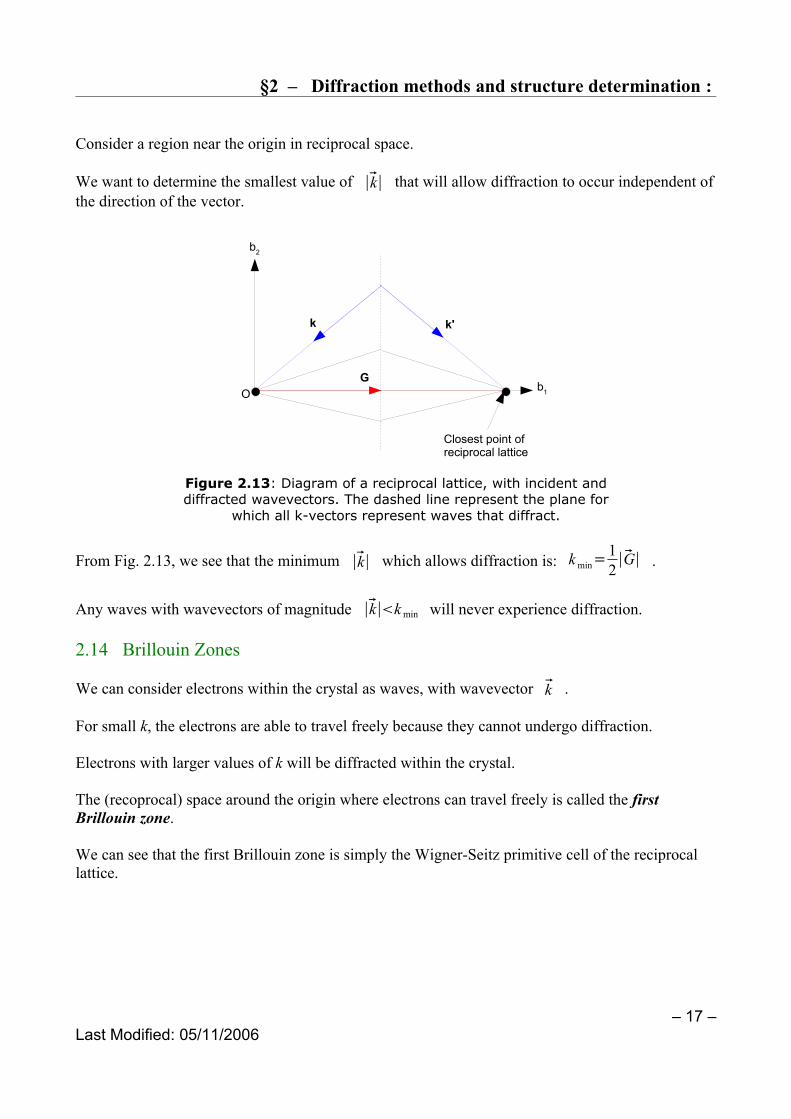
Consider a region near the origin in reciprocal space.

We want to determine the smallest value of ∣k∣ that will allow diffraction to occur independent of the direction of the vector.

From Fig. 2.13, we see that the minimum ∣k∣ which allows diffraction is: kmin=12∣G∣ .

Any waves with wavevectors of magnitude ∣k∣kmin will never experience diffraction.

2.14 Brillouin Zones

We can consider electrons within the crystal as waves, with wavevector k .

For small k, the electrons are able to travel freely because they cannot undergo diffraction.

Electrons with larger values of k will be diffracted within the crystal.

The (recoprocal) space around the origin where electrons can travel freely is called the first Brillouin zone.

We can see that the first Brillouin zone is simply the Wigner-Seitz primitive cell of the reciprocal lattice.

– 17 –Last Modified: 05/11/2006

Figure 2.13: Diagram of a reciprocal lattice, with incident and diffracted wavevectors. The dashed line represent the plane for

which all k-vectors represent waves that diffract.

k k'

GO b1

b2

Closest point ofreciprocal lattice


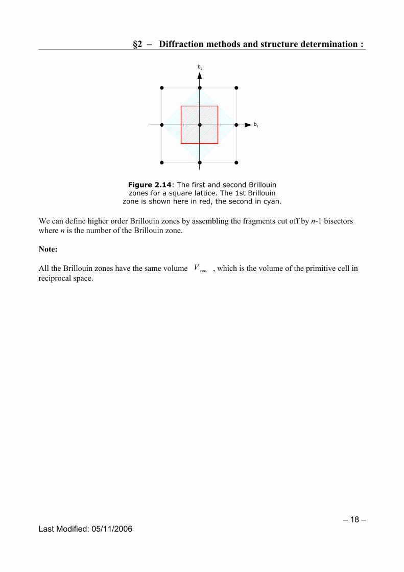
We can define higher order Brillouin zones by assembling the fragments cut off by n-1 bisectors where n is the number of the Brillouin zone.

Note:

All the Brillouin zones have the same volume V rec. , which is the volume of the primitive cell in reciprocal space.

– 18 –Last Modified: 05/11/2006

Figure 2.14: The first and second Brillouin zones for a square lattice. The 1st Brillouin

zone is shown here in red, the second in cyan.

b2

b1

§2 – diffraction methods and structure determination

Documents