2. Definitions and Methods

2.1

JD 2008

2.2

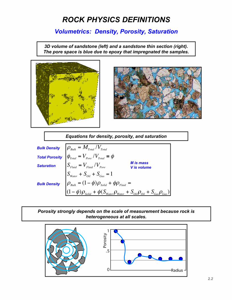
ROCK PHYSICS DEFINITIONSVolumetrics: Density, Porosity, Saturation

Radius

Porosity

0

1

.5

3D volume of sandstone (left) and a sandstone thin section (right).The pore space is blue due to epoxy that impregnated the samples.

Equations for density, porosity, and saturation

Porosity strongly depends on the scale of measurement because rock isheterogeneous at all scales.

Bulk Density

Total Porosity

Saturation

Bulk Density

€

ρBulk = MTotal /VTotal

φTotal =VPore /VTotal ≡ φ

SFluid =VFluid /VPore

SWater + SOil + SGas =1ρBulk = (1−φ)ρSolid + φρFluid =

(1−φ)ρSolid + φ(SWaterρWater + SOilρOil + SGasρGas)

M is massV is volume

2.3

ROCK PHYSICS DEFINITIONSVelocity

2.4

ROCK PHYSICS BASICSNormal Reflection

Ip = ρV p

ν =

12

(Vp / Vs )2 − 2

(Vp / Vs )2 − 1

1200

1300

1400

1500

1600

1700

1800

1900

2000

Trav

el T

ime

(ms)

NormalReflection

T

R

R(0)=

Ip2 − Ip1Ip2 + Ip1

=dIp2Ip

=12d ln Ip

Two important elastic parameters that affect reflection are derived from velocityand density. They are the acoustic (or P-) impedance Ip and Poisson’s ratio ν

Normal Incidence. The reflection amplitude of a normal-incidence P-wave at theinterface between two infinite half-spaces depends on the difference between the

impedances of the half-spaces. The same law applies to S-wave reflection.

A reflection seismogram is a superposition ofsignals reflected from interfaces between earth

layers of different elastic properties.

It is useful, therefore, to examine reflection at asingle interface between two elastic half-spaces.

Normal reflection forms a full differential. Therefore, it can be integrated toarrive at the absolute values of P-wave impedance. This procedure is called

impedance inversion.

Zoeppritz (1919)

2.5

ROCK PHYSICS BASICSReflection at an Angle

IncidentP-Wave Reflected

P-Wave

ReflectedS-Wave

TransmittedS-Wave

TransmittedP-Wave

Θ1

Θ2

Φ1

Φ2

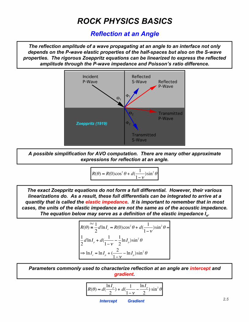
The reflection amplitude of a wave propagating at an angle to an interface not onlydepends on the P-wave elastic properties of the half-spaces but also on the S-wave

properties. The rigorous Zoeppritz equations can be linearized to express the reflectedamplitude through the P-wave impedance and Poisson’s ratio difference.

A possible simplification for AVO computation. There are many other approximateexpressions for reflection at an angle.

The exact Zoeppritz equations do not form a full differential. However, their variouslinearizations do. As a result, these full differentials can be integrated to arrive at a

quantity that is called the elastic impedance. It is important to remember that in mostcases, the units of the elastic impedance are not the same as of the acoustic impedance.

The equation below may serve as a definition of the elastic impedance Ie.

Parameters commonly used to characterize reflection at an angle are intercept andgradient.

Intercept Gradient

€

R(θ) ≈ R(0)cos2θ + d( 11−ν

)sin2θ

€

R(θ) ≡Def 12d ln Ie ≈ R(0)cos

2θ + d( 11−ν

)sin2θ =

12d ln Ip + d( 1

1−ν−12ln Ip )sin

2θ

⇒ ln Ie = ln Ip + ( 21−ν

− ln Ip )sin2θ

€

R(θ) ≈ d(ln Ip2) + d( 1

1−ν−ln Ip2) sin2θ

Zoeppritz (1919)

2.6

ROCK PHYSICS BASICSReflection at an Angle

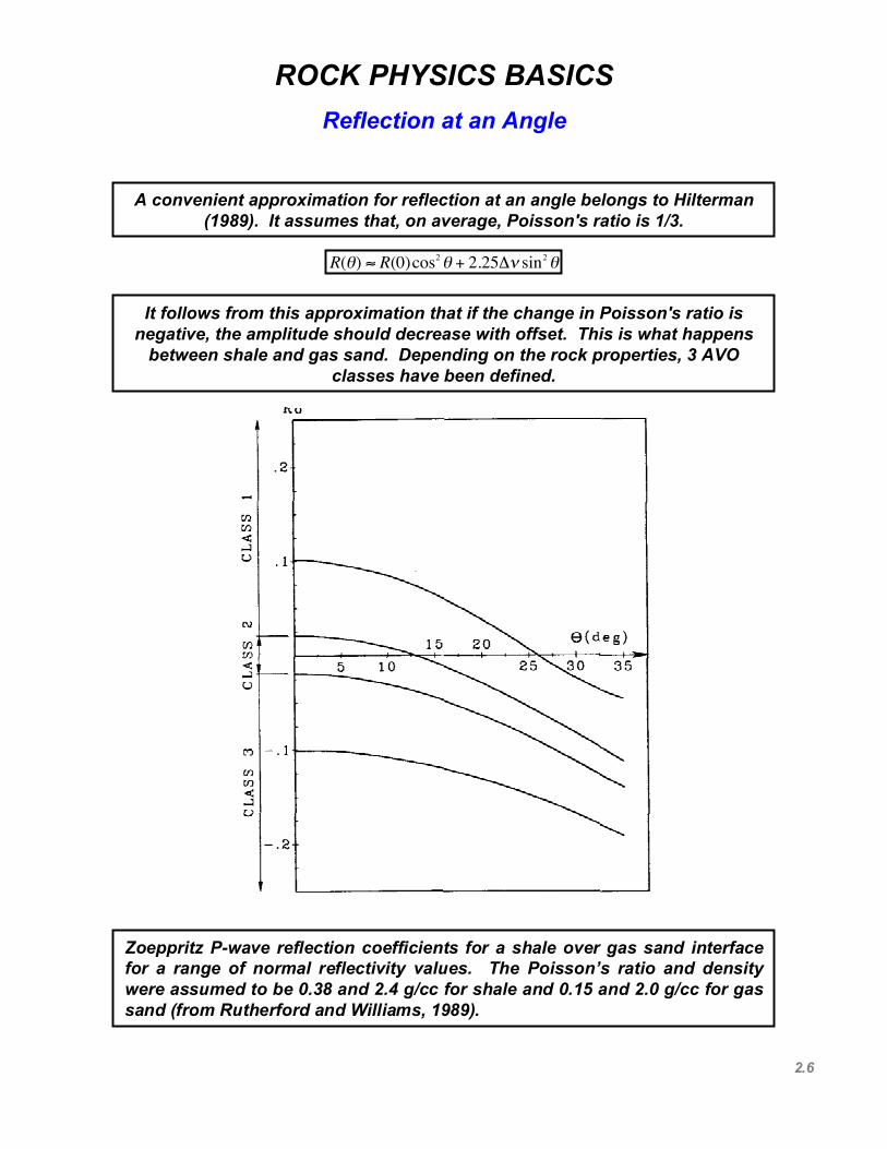
A convenient approximation for reflection at an angle belongs to Hilterman(1989). It assumes that, on average, Poisson's ratio is 1/3.

It follows from this approximation that if the change in Poisson's ratio isnegative, the amplitude should decrease with offset. This is what happens

between shale and gas sand. Depending on the rock properties, 3 AVOclasses have been defined.

Zoeppritz P-wave reflection coefficients for a shale over gas sand interfacefor a range of normal reflectivity values. The Poisson’s ratio and densitywere assumed to be 0.38 and 2.4 g/cc for shale and 0.15 and 2.0 g/cc for gassand (from Rutherford and Williams, 1989).

€

R(θ) ≈ R(0)cos2θ + 2.25Δν sin2θ

2.7

ROCK PHYSICS BASICSRelative Impedance Inversion

€

Rpp (θ) ≈ Rpp (0) cos2θ + 2.25Δν sin2θ

≈ Rpp (0) + [2.25Δν − Rpp (0)]sin2θ,

€

Rpp(0) =Ip 2 − Ip1Ip 2 + Ip1

=dIp2Ip

=12d ln Ip ,

€

Ip = exp[2 Rpp(0)dz∫ ].

€

Δν =Rpp(θ )− Rpp(0) cos

2θ

2.25sin2θ,

ν =Rpp(θ )− Rpp(0) cos

2θ

2.25sin2θ∫ dz.

2.8

ROCK PHYSICS BASICSRelative Impedance Example

Relative seismically-derived impedance and Poisson's ratio donot provide the absolute values of these elastic constants.However, they are often useful in obtaining spatial shapes ofimpedance and Poisson's ratio.

2.9

ROCK PHYSICS BASICSElasticity

Ti = σ ijn j

Stress Tensor

u

x1

x2

x3

x1

Tn

x2

x3

Strain Tensor

ε ij =

12(∂ui∂x j

+∂uj∂xi

)

σ ij = σ ji i ≠ j; ε ij = ε ji i ≠ j.

σ ij = cijklekl; cijkl = cjikl = cijlk = cjilk, cijkl = cklij .

σ ij = λδ ijεαα + 2µε ij; ε ij = [(1 + ν )σ ij − νδ ijσαα ]/ E.

Commonly used constants are: λ and µ -- Lame's constants; ν -- Poisson's ratio; E -- Young's modulus. The elasticmoduli are determined by the experiment performed. For example, the bulk modulus is measured in thehydrostatic compression experiment. The shear modulus is measured in the shear deformation experiment.

Stress and strain. Forces acting within a mechanical body are mathematicallycharacterized by the stress tensor which is a 3x3 matrix. By using a stress tensor wecan find the vector of traction acting on an elemental plane of any orientation withinthe body (figure on the left).

The deformation within the body is characterized by the strain tensor. This tensor isformed by the derivatives of the components of the displacement of a material point inthe body (figure on the right).

Both stress and strain tensors are symmetrical matrices.

Hooke’s law relates stress to strain. It postulates that this relation is linear. In general, there are 21 independentelastic constants that linearly relate stress to strain.

Fortunately, if a body is isotropic, only two independent elastic constants are required. These constants arecalled elastic moduli.

Elastic moduli derived from loading experiments are called static moduli

Bulk Modulus

K = λ + 2µ / 3

Z

X

Y

σ xz = 2µε xz

ε xx = εyy = εzz = ε xy = 0

Shear

Shear Modulus Compressional Modulus

Hydrostatic Loading Distortion, no volumechange

No lateral deformation

€

M = K + (4 /3)µ

2.10

ROCK PHYSICS BASICSElastic-Wave Velocity

An elastic stress wave can propagate through an elastic body and generate stress andstrain disturbance. The magnitude of deformation generated by a propagating wave isusually very small, on the order of 10-7. As a result, the stress perturbation is alsovery small, much smaller than the ambient state of stress.

The speed of an elastic wave is related to the elastic moduli via the wave equation(below) where u is displacement, t is time, z is the spatial coordinate, M is the elasticmodulus, and ρ is the density.

u(z)

σ(z+dz)σ(z) zdzA

∂ 2u∂ t2

=Mρ∂ 2u∂z2

It follows from the wave equation that the speed of wave propagation is

M / ρ

Vp = M / ρ = (K + 4G / 3) / ρ

Vs = G / ρ

M = ρVp2 ; G = ρVs

2 ; K = ρ(V p2 − 4Vs

2 / 3); λ = ρ(Vp2 − 2Vs

2 ).

M is the compressional modulus or M-modulusG (or µ) is the shear modulusK is the bulk modulusE is Young’s modulusν is Poisson’s ratioλ is Lame’s constant

ν =

12

(Vp / Vs )2 − 2

(Vp / Vs )2 − 1

Elastic moduli derived from velocity data are called dynamic moduli

Poisson’s Ratio

€

ν =12(Vp /Vs)

2 − 2(Vp /Vs)

2 −1

2.11

ROCK PHYSICS BASICSRelations between Elastic Constants

Poisson’s ratio relates to the ratios of various elastic moduli and elastic-wave velocities.

ν =12(V p / Vs )

2 − 2(V p / Vs )

2 −1=12M / G − 2M / G −1

=12K / G − 2 / 3K / G +1 / 3

=12

λ / Gλ / G +1

Theoretically, PR may vary between -1 and 0.5

−1 ≤ ν ≤ 0.5

ν = −1⇒ M =43G; Vp =

23Vs ; K = 0; λ = −

23G

ν = 0⇒ M = 2G; Vp = 2Vs ; K =23G; λ = 0

ν = 0.5⇒Vs = 0|K = ∞

Sometimes, the dynamic PR of dry sand at low pressure may appear negative.

Plot below shows PR versus porosity in dry unconsolidated sand at low differentialpressure. This may mean (a) wrong data or (b) anisotropic rock.

0.0

0.1

0.2 0.3 0.4

Pois

son'

s Ra

tio

Porosity

Room-Dry Sands5 MPa

2.12

ROCK PHYSICS BASICSStatic and Dynamic Moduli

Log Strain

Stre

ss

10-7 10-2

DYN

AM

IC

STATIC

Load

Unload

By definition, the dynamic moduli of rock are those calculated from the elastic-wave velocity and density. The static moduli are those directly measured in adeformational experiment.

The static and dynamic moduli of the same rock may significantly differ from eachother. The main reason is likely to be the difference in the deformation (strain)amplitude between the dynamic and static experiments.

In the dynamic wave propagation experiment the strain is about 10-7 while staticstrain may reach 10-2.

σ Stress

Axial Strainεa

εrE = σ / εa

ν = εr / εa

Typical Plastic Behavior

RadialStrain

2.13

ROCK PHYSICS BASICSNeed for Static Moduli

2c

2b

SHmin

P

b = 2c 1 − ν2

E(P − SHmin)

Importance of Static Young'sModulus and Poisson's Ratio

for Hydrofracture Design

Static moduli are often used in wellbore stability and in-situ stress applicationsto evaluate the possibility of breakouts, elevated pore pressure, and tectonicstress distribution. For example, a common method of calculating the horizontalstress in earth is by assuming that the earth is elastic and does not deform in thehorizontal direction.

SH

SVSH = SV

ν1 − ν

Vertical(Overburden)

Stress

HorizontalStress

Poisson’sRatio

Hydrofracture can be approximated by a 2D elliptical crack who's dimensionsdepend on the static Young's modulus and Poisson's ratio.

2.14

ROCK PHYSICS BASICSStatic and Dynamic Moduli in Sand

ν =

12

(Vp / Vs )2 − 2

(Vp / Vs )2 − 1

Porosity (left) and velocity (right) versus pressure in high-porosity room-dry sandsample from the Gulf of Mexico.

Zimmer, M., 2003, Doctoral Thesis, Stanford University .

Velocity versus porosity (left) and dynamic and static bulk moduli calculated for thesame sample.

0.35

0.36

0.37

0.38

0.39

0.40

0 5 10 15 20

Poro

sity

Pressure (MPa)

POMPONIO

0.2

0.4

0.6

0.8

1.0

1.2

1.4

1.6

1.8

0 5 10 15 20

Vel

ocity

(km

/s)

Pressure (MPa)

POMPONIO

SAND

SAND

0.2

0.4

0.6

0.8

1.0

1.2

1.4

1.6

1.8

0.36 0.38 0.4

Vel

ocity

(km

/s)

Porosity

POMPONIOP

S

SAND

0

1

2

3

4

0 5 10 15 20

Bulk

Mod

ulus

(GP

a)

Pressure (MPa)

POMPONIO

Static

Dynamic

SAND

CREEP

2.15

ROCK PHYSICS BASICSCompaction Effects in Sand/Shale

Yin, H., 1992, Doctoral Thesis, Stanford University .

Velocity in shale depends on stress and porosity and deformationhistory.

SAND/CLAY SAND/CLAY

SAND/CLAY

SAND/CLAY

Load

Load

LoadUnload

Unload

Unload

Unload

Load

2.16

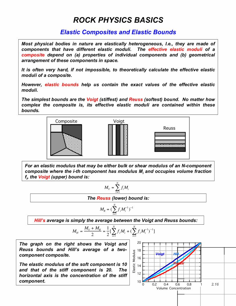
ROCK PHYSICS BASICSElastic Composites and Elastic Bounds

Most physical bodies in nature are elastically heterogeneous, I.e., they are made ofcomponents that have different elastic moduli. The effective elastic moduli of acomposite depend on (a) properties of individual components and (b) geometricalarrangement of these components in space.

It is often very hard, if not impossible, to theoretically calculate the effective elasticmoduli of a composite.

However, elastic bounds help us contain the exact values of the effective elasticmoduli.

The simplest bounds are the Voigt (stiffest) and Reuss (softest) bound. No matter howcomplex the composite is, its effective elastic moduli are contained within thesebounds.

Composite VoigtReuss

For an elastic modulus that may be either bulk or shear modulus of an N-componentcomposite where the i-th component has modulus Mi and occupies volume fractionfi, the Voigt (upper) bound is:

MV = fiMii=1

N

∑

MR = ( f iMi−1

i=1

N

∑ )−1

The Reuss (lower) bound is:

Hill’s average is simply the average between the Voigt and Reuss bounds:

MH =MV + MR

2=12[ f iMii=1

N

∑ + ( f iMi−1

i=1

N

∑ )−1]

10

12

14

16

18

20

0 0.2 0.4 0.6 0.8 1

Elas

tic M

odul

us

Volume Concentration

The graph on the right shows the Voigt andReuss bounds and Hill’s average of a two-component composite.

The elastic modulus of the soft component is 10and that of the stiff component is 20. Thehorizontal axis is the concentration of the stiffcomponent.

Voigt

Reuss

Hill

2.17

ROCK PHYSICS BASICSHashin-Shrikman Elastic Bounds

For an isotropic composite, the effective elastic bulk and shear moduli arecontained within rigorous Hashin-Shtrikman bounds. These bounds have beenderived for the bulk and shear moduli. The Hashin-Shtrikman bounds are tighterthan the Voigt-Reuss bounds.

[ fiKi + 4

3Gmini=1

N

∑ ]−1 − 43Gmin ≤ Keff ≤ [

fiKi + 4

3Gmax]−1

i=1

N

∑ −43Gmax,

[ fi

Gi +Gmin6

9Kmin + 8Gmin

Kmin + 2Gmin

]−1i=1

N

∑ −Gmin6

9Kmin + 8GminKmin + 2Gmin

≤ Geff ≤

[ fi

Gi +Gmax6

9Kmax + 8GmaxKmax + 2Gmax

i=1

N

∑ ]−1 − Gmax

69Kmax +8Gmax

Kmax + 2Gmax

,

In the Hashin-Shtrikman equations, the subscript “eff” is for the effective elasticbulk and shear moduli. The subscripts “min” and “max” are for the softest andstiffest components, respectively.

A physical realization of the Hashin-Shtrikman bounds for two components is theentire space filled by composite spheres of varying size. The outer shell of eachsphere is the softest component for the lower bound and the stiffest component forthe upper bound.

If one of the components is void (empty pore) the lower bound is zero.

Hashin-ShtrikmanBounds: Realization

10

12

14

16

18

20

0 0.2 0.4 0.6 0.8 1

Elas

tic M

odul

us

Volume Concentration

Voigt

Reuss

Hashin-Shtrikman

2.18

ROCK PHYSICS BASICSElastic Bounds for Water-Saturated Sand

Unfortunately, if the elastic moduli of the two components of the compositeare very different, the bounds lie very far apart.

They cannot be used for practical velocity prediction.

In the example below, plotted is velocity versus porosity as calculated for aquartz/water mixture using the elastic bounds. The data points are for water-saturated sandstones. The data lie within the elastic bounds curves.

The bounds can still be used to quality control of the data.

1

2

3

4

5

6

0 0.2 0.4 0.6 0.8 1

Vp

(km

/s)

Porosity

Voigt

Reuss

UpperHashin-Shtrikman

1

2

3

4

5

6

0 0.2 0.4 0.6 0.8 1

Vp

(km

/s)

Porosity

Voigt

Reuss

UpperHashin-Shtrikman

In the example below, the red data points lie below the lower bound curve forthe quartz/water mix. The reason is that these data are for gas-saturatedsands.

2.19

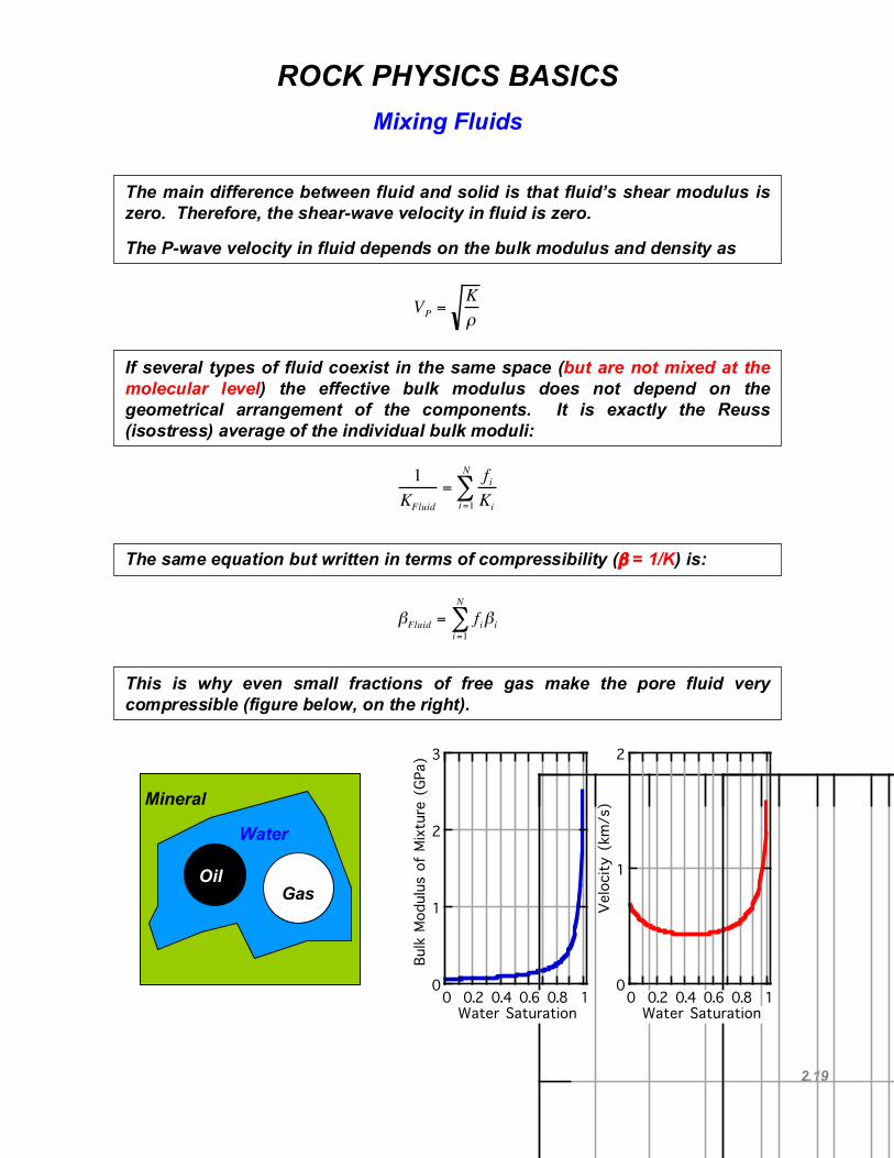
ROCK PHYSICS BASICSMixing Fluids

The main difference between fluid and solid is that fluid’s shear modulus iszero. Therefore, the shear-wave velocity in fluid is zero.

The P-wave velocity in fluid depends on the bulk modulus and density as

VP =Kρ

If several types of fluid coexist in the same space (but are not mixed at themolecular level) the effective bulk modulus does not depend on thegeometrical arrangement of the components. It is exactly the Reuss(isostress) average of the individual bulk moduli:

1KFluid

=fiKii=1

N

∑

The same equation but written in terms of compressibility (β = 1/K) is:

βFluid = fii=1

N

∑ βi

This is why even small fractions of free gas make the pore fluid verycompressible (figure below, on the right).

Mineral

Water

OilGas

0

1

2

3

0 0.2 0.4 0.6 0.8 1

Bulk

Mod

ulus

of

Mix

ture

(GP

a)

Water Saturation

0

1

2

0 0.2 0.4 0.6 0.8 1

Vel

ocity

(km

/s)

Water Saturation

2.20

ROCK PHYSICS BASICSPressure and Rock Properties

1.5

2.0

2.5

3.0

3.5

4.0

0 5 10 15 20 25

Vel

ocity

(km

/s)

Confining Pressure (MPa)

In-SituStress

Vp

Vs

When rock is extracted from depth and re-loaded in the lab, it exhibits a strongvelocity-pressure dependence, especially at low confining pressure. The primaryreason is microcracks that open during in-situ stress relief.

Below: Vp and Vs versus confining pressure in room-dry sandstone samples. Thein-situ effective stress is about 15 MPa. Different colors correspond to differentsamples.

2.21

ROCK PHYSICS BASICSPressure and Rock Properties

Phenomenology of pressure effect on velocity in room-dry sandstonedataset.

The velocity-porosity trends become sharper as pressure increases.

2

3

4

5

6

0 0.1 0.2 0.3

Vp

(km

/s)

Porosity

5 MPa

0 0.1 0.2 0.3Porosity

20 MPa

0 0.1 0.2 0.3Porosity

40 MPa

2.22

ROCK PHYSICS BASICSPressure and Rock Properties

Phenomenology of pressure effect on velocity in room-dry sandstonedataset.

Both Vp and Vs may significantly change with changing pressure.

1

2

3

4

5

6

1 2 3 4 5 6

Vp

at 4

0 M

Pa (

km/s

)

Vp at 5 MPa (km/s)

1

2

3

4

1 2 3 4

Vs

at 4

0 M

Pa (

km/s

)

Vs at 5 MPa (km/s)

Vp Vs

Vs at 5 MPa

Vs a

t 40

MPa

Vp at 5 MPa

Vp a

t 40

MPa

2.23

ROCK PHYSICS BASICSPressure and Rock Properties

The Vp and Vs versus pressure changes are not necessarily scalable -- theVp/Vs ratio and Poisson's ratio change as well.

0

0.1

0.2

0.3

0 0.1 0.2 0.3

PR a

t 40

MPa

PR at 5 MPa

Poisson'sRatio

PR at 5 MPa

PR a

t 40

MPa

2.24

ROCK PHYSICS BASICSPressure and Rock Properties

The effect of pressure on porosity is not as large as on velocity. The mainreason is that rock's elasticity is affected by thin compliant cracks that donot occupy much of the pore space volume.

.1

.2

.3

.1 .2 .3Porosity at 5 MPa

40 MPa

Poro

sity

at

40 M

Pa

0

.01

.1 .2 .3Porosity at 5 MPa

Poro

sity

Incr

ease

0

.1

.2

.1 .2 .3Porosity at 5 MPa

Rela

tive

Chan

ge

5 MPa to 40 MPaRelative Reduction

€

Δφφ

2.25

ROCK PHYSICS BASICSStress-Induced Anisotropy

θ

€

Vp (θ) ≈α(1+ δ sin2θ cos2θ + εsin4 θ)

VsV (θ) ≈ β[1+α 2

β 2(ε −δ)sin2θ cos2θ]

VsH (θ) ≈ β[1+ γ sin2θ]

€

ε =Vp (π /2) −Vp (0)

Vp (0)γ =

VsH (π /2) −VsV (π /2)VsV (π /2)

=VsH (π /2) −VsH (0)

VsH (0)

Thomsen's anisotropic formulation (weak transverse isotropy)

Vzz

VyyVxx Vyz

VyxVxz

Vxy

Vzy

Vzx

ZY

XVzz

Vxx

Vyy

Vyz

Vyx

Vxz

Vzy

Vxy

Vzx

Ottawa sand. Uniaxial compression.Pxx = Pyy = 1.72 bar. Yin (1992).

Anisotropic stress field induces anisotropy in otherwise isotropic rock.

2.26

ROCK PHYSICS BASICSPermeability

Permeability is a fluid flow property of a porous medium. Its definition comesfrom Darcy’s law which states that the flow rate is linearly proportional to thepressure gradient.

Q = −kAµΔPL

FlowRate

PressureHead

SampleLengthViscosity

SampleCross-SectionPERMEABILITY

2.27

ROCK PHYSICS BASICSPermeability -- Kozeny-Carman Equation

Permeability depends on porosity and grain size.

Kozeny-CarmanEquation (SI UNITS)

€

kd2

=172

φ 3

(1−φ)2τ 2

Permeability

Grain Size Tortuosity

Porosity

Permeability may be almost zero in carbonate where large vuggy pores are not connected.This pore geometry is a topological inverse of the pore geometry of clastic sediment.Permeability equations that work in clastics may not work in carbonates.

Drastic drop in permeability asporosity increases but claycontent increases too (grainsize decreases). Yin (1992).

Permeability depends on porosity and grain size and also (critically) on thepore-space geometry.

2.28

ROCK PHYSICS BASICSPermeability and Stress

Permeability in medium-to-high porosity clastic sediment is weakly dependent on stress.

0.1

0.2

0.3

0.1 0.2 0.3

Poro

sity

at

4000

psi

Porosity at 400 psia

1

10

100

1 10 100

Perm

eabi

lity

(mD)

at

4000

psi

Permeability (mD) at 400 psib

Ali Mese (1998) Ali Mese (1998)

Walls (1982)

Permeability in tight sandstone samples. Porosity 0.03 to 0.07.

Relative changes of high permeability with pressure are smaller than those forlow permeability. Both may have implications for fluid transport.

2.29

€

U1

€

U2

€

I

€

U =U1 −U2

R =U /IPotential

Drop

ElectricalCurrent

Resistance

€

ρ = RA / l

Resistivity

€

[R] =Ω≡Ohm[ρ] =Ω⋅m ≡Ohm ⋅m

€

σ =1/ρ

Conductivity

DEFINITIONS OF RESISTIVITY

0.1

1

10

100

6000 6500 7000 7500 8000

Rt (

Ohm

m)

Depth (ft)

0

50

100

150

6000 6500 7000 7500 8000

GR

Depth (ft)