Lagrangian Trajectory Modeling of Lunar Dust Particles

John E. Lane', Philip T. Metzger2 , and Christopher D. Immer3 1,3ASRC Aerospace, MD: ASRC-15, Kennedy Space Center, FL 32899

John.Lane- 1 (ksc.nasa.gov, Christoi,her.D.Immer(ksc.nasa.gov

2NASAJJ'SC Granular Mechanics and Surface Systems Laboratory, KT-D3, Kennedy Space Center, FL 32899

Philip.T.Metzger@nasa.gov

INTRODUCTION

Apollo landing videos shot from inside the right LEM window, provide a

quantitative measure of the characteristics and dynamics of the ejecta spray of

lunar regolith particles beneath the Lander during the final 10 [m] or so of descent.

Photogrammetry analysis gives an estimate of the thickness of the dust layer and

Pressure Exit (Space) I

IT

a) ()

U)

CU C.)

a)

.:.IuIII I -.

I!jI -EE--

•III!'II:i li H

WaltI

rocket 11 ii

motor 'II iI Pressure 1 Exit tt

I I PaP II liii Hill

rocket - I nozzle 1? t liii HI Ii I

IT Ill I hI .1' I II i I I I - . 11111111 I I lit I ii

I llI.jII liii II I 111111111 II. I .- J.I. Hi II I II I I II

Axis of H I i IrIlI.i I f Symmetry I I I

II I'! I II I • I I I I. II - Ii 1111. il l iii Iii I

1 . .

Wall (Lunar Surface)

,i aii

2 4 6 8 10 Horizontal Distance. y [m]

Figure]. 2D CFD boundary and grid point definition.

6 -, T ̂ 5

4

A

El

https://ntrs.nasa.gov/search.jsp?R=20130012062 2018-06-17T13:16:34+00:00Z

angle of trajectory (Immer, 2008). In addition, Apollo landing video analysis

divulges valuable information on the regolith ejecta interactions with lunar surface

topography. For example, dense dust streaks are seen to originate at the outer rims

of craters within a critical radius of the Lander during descent.

The primary intent of this work was to develop a mathematical model and

software implementation for the trajectory simulation of lunar dust particles acted

on by gas jets originating from the nozzle of a lunar Lander, where the particle

sizes typically range from 10 m to 500 pm. The high temperature, supersonic jet

of gas that is exhausted from a rocket engine can propel dust, soil, gravel, as well

as small rocks to high velocities. The lunar vacuum allows ejected particles to

travel great distances unimpeded, and in the case of smaller particles, escape

velocities may be reached. The particle size distributions and kinetic energies of

ejected particles can lead to damage to the landing spacecraft or to other hardware

that has previously been deployed in the vicinity. Thus the primary motivation

behind this work is to seek a better understanding for the purpose of modeling and

predicting the behavior of regolith dust particle trajectories during powered rocket

descent and ascent.

#&---Lunar Lander (Orion)ALr Lander (Orion) Rocket Nozzle

Ri 'Ri Rocket Nozzle

I Is

Lunar Crater pRn Rocket Exhaust

Main Blast Area25 Pis

Rn

40 Pis

Pis

Rocket Exhaust Lunar Crater

Main Blast Area

Figure 2. 3D DSMC simulation geometry.

COMPUTATIONAL STRATEGY

The trajectory model described in this paper requires output from a two- or three-

dimensional fluid dynamics simulation of the rocket nozzle exhaust. Traditionally,

this is achieved using a commercially available computationaifluid dynamics

(CFD) software package. Alternatively, direct simulation Monte Carlo (DSMC)

software may be employed. DSMC simulators model fluid flows using a large

number of discrete molecules in a Monte Carlo fashion to solve the Boltzmann gas

equation. The worked described in this paper utilizes both CFD and DSMC

simulations of an Apollo-like lunar Lander. In the case of the CFD simulations,

2D symmetry was exploited based on cylindrical symmetry where the problem is

independent of azimuth angle, reducing complexity and computation time (see

Figure 1). Full 3D geometries were processed by DSMC software, as depicted in

Figure 2, where no symmetries were assumed.

The CFD/DSMC output provides estimates of gas density p(r), gas velocity u(r),

and gas temperature T(r) for a gridded volume described by r vector points in the

bounded domain. These values are interpolated from the CFD/DSMC grid by

finding four nearest grid neighbors in a volume around the kth trajectory point and

applying an N-dimensional interpolation algorithm. Inputs which are initial

conditions of the trajectory calculation include the particle diameter D and initial

position of the particle r0 = (xo, yo, z0) where the vertical direction x is positive up

and equal to zero at the surface. Typically, the particle starting position above the

surface is set by the user as x0.

MATHEMATICAL MODEL AND TRAJECTORY ALGORITHM

For a particle of diameter D and mass m, the trajectory is due to three external

forces: lunar gravity, jet gas drag, and lift caused by the gas flow. The sum of

external forces is equal to the acceleration experienced by the particle, which can

be estimated by a Taylor series expansion about time point k, resulting in a set of

difference equations for position and velocity:

Vk = V k I -FakIAt

r, =r,_ 1 +vk_lL\t+--ak_lL\t

U k =u(rk)

Pk =p(rk)

(1)

ak - 2rCD D2 -

8m lU k —vkI.(uk Vk)Pk +aLfl +gê

_ffCDD2[D3PLJUk_vk.(Uk_vk)pk+aLJ+gLeL

- 8

= 3 CD,okUk VkI(Uk —vk)+ a L ?fl +ge

4DpL

9L is lunar gravity and PL is the lunar soil particle density (3100 [kg m 3]); p(r)

is the gas density and u(r) is the gas velocity from the CFD/DSMC files (*.g and

*.q files). These values are computed by finding nearest neighbors in a volume

around the point of interest and applying the spatial interpolation algorithm of

Shepard (1968).

aLfl is the lift acceleration due to the vertical gradient of the horizontal component

of gas flow (Shao, 2000):

3CLpkI a aLfi k - VkI - I U k - VkIh. (2)

2PL ax

where CL is the coefficient of lift.

The direction of the lunar gravity unit vector is given by:

(RL +X"\ —1 I I

eL- I y I (3)

,I(RL+x)2+y2+z2z J

where the lunar gravity constant 9L is defined at the surface of a sphere of radius

RL (moon radius).

The coefficient of drag, CD is a function of the Reynolds number, R:

R Dpklu k — vkl

k AI1

where T is the static temperature of the gas at the kth position of the particle,. The

empirical parameters in the denominator are: A = 1.71575x 10 -7 and fl = 0.78.

The coefficient of drag is computed from the following empirical formula:

(4)

24.0R' R <2

CD = 18.5R° 6 2:!^R<500

0.44 R'::^500

The initial conditions are:

V 0 =0

r0 = R0

Uo = u(r0)

po =p(r0)

3CDPO+

3CLPk I U 0I horiz

a IUOIh . +ge

a0= 4DPL 210L ax

(5)

(6)

SIMULATION EXPERIMENTS

Numerous gas jet simulations involving variations of rocket nozzle height above

ground, nozzle angles, and number of craters at various distances and diameters,

were run using DSMC software. Some of these variations are depicted in the

schematic of Figure 2. The DSMC output then became the particle trajectory

model (PTM) input, where PTM is a FORTRAN code implementation of

Equations (1) through (6). These results were reported in detail by Metzger

(2007).

For the purpose of this present work, only CFD output is used as inputs to PTM.

The four CFD test cases used in the trajectory simulation experiments are

summarized in Tables 1.

Table 1. CFD Cases used as Inputes to PTM

Distance from Nozzle Center Line to Crater Center, R

Height of Nozzle above Surface, h SRN 15 RN

2.5 RN Case C2

5 R Case C7 Case C3

10 RN Case Ci

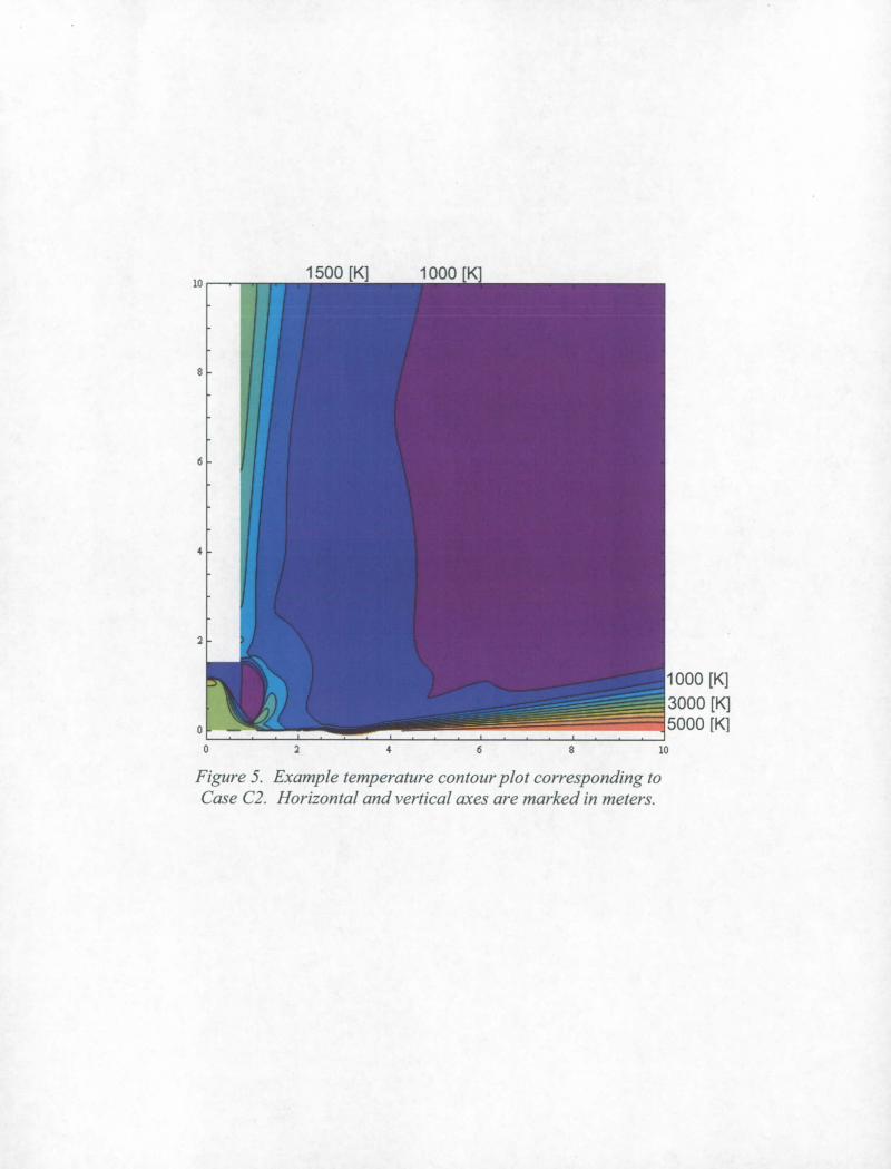
Figures 3, 4, and 5 display the CFD Case 2 output array values needed for input to

PTM, i.e., gas density, gas velocity, and gas temperature.

Table 2. Example PTM input parameters.

D [pm] x [m] y [m] z [m] At [ps] NL CL Particle Initial Initial Not used Time step Number of Coefficient diameter vertical Pt radial pt in 2D- iterations of lift

above from CFD case ground

nozzle

50 0.003 3.7762 0 1000 500 20

Table 3. PTM time step versus particle diameter.

D[im] 10 25 1 50 100 250 500

At[ts] 200 500 1000 2000 5000 10000

Figure 6 shows the PTM output for six particle sizes given by Table 3, spanning

the range of lunar dust particle sizes. The initial starting coordinate in Table 2 is

used in all six runs and corresponds to a point 3 [mm] above the outer lip of the

crater. The reason for choosing a point slightly above the ground will be

discussed in the following section. Similar plots are generated for the other cases

shown in Table 1.

In order to compare results from the four CFD cases studied above, the velocity

vector corresponding to the trajectories of each of the six particle sizes is

calculated from the trajectory data. The horizontal right boundary at 10 [m] is a

convenient point to evaluate velocity. Figure 8 is a particle velocity magnitude

(speed) plot of three CFD cases, corresponding to three rocket nozzle heights, h,

above the ground compared with DSMC data from Metzger (2007). Figure 9 is

the particle velocity angles relative to the ground for the three CFD cases.

PTM plots for six particle sizes is shown in Figure 7, corresponding to Case C3.

In Case C3, the crater is located at 15RN 30 [ft]. Initializing the starting point of

the particles according to Table 2, results in velocities with lower angles and

speeds. This result is a consequence of the turbulence generated above the crater,

slowing down the particle with a downward component of velocity.

10

0 2 4 6 8 10

Dtristy (kg

5x103

3X10 -x10

Figure 3. Example gas density plot corresponding to CFD Case C2. Horizontal and vertical axes are marked in meters.

10

Velocity (m1

3200

I 0 2

10

Figure 4. Example gas velocity plot corresponding to CFD Case C2. Horizontal and vertical axes are marked in meters.

10

1000 [K]

3000 [K] 5000 [K]

U 4 U 10

Figure 5. Example temperature contour plot corresponding to Case C2. Horizontal and vertical axes are marked in meters.

tth/ [kg 3]

"X 10 mis]

0o [m/s]

-

ijX10-7

3000 2500 2000 1500 Im/si Im/si [rn/si [rn/si

0 2 4 6 8 10

Figure 6. PTM output for CFD Case 2 and initial values from Table 2. Horizontal and vertical axes are marked in meters.

03

0.2

0.1

0.0

-0.1

2500

2500

1500 [rn/si

2000 [m/s)

[rn/si

10

Figure 7. PTMoutput for CFD Case 3 and initial values from Table 2. Horizontal and vertical axes are marked in meters.

1400

1200

1000

800

> 600

400

200

0

-0- CFD:Case Cl -0- CFD:Case C2

CFD: Case 07 SMC Avg

455789 2 3 45 10 100

D [urn]

Figure 8. Particle speeds exiting the CFD boundary for various particle sizes and CFD Cases of Table 1. The solid black line is averaged data from Metzger (2007).

5

-0- CFD Case Cl -0-- CED Case 02

CED Case 07 - DSMC Avg

S

2 J 4 55189 2 3 4 5 10 100

D [urn]

Figure 9. Particle trajectory angles relative to ground corresponding to Figure 7. Again, the solid black line is averaged data from Metzger (2007).

4

0) a)

0) C 4:

1

DISCUSSION AND CONCLUSIONS

The particle velocities converge nicely for sizes in the range of 200 to 500 [im},

as shown by Figure 8. For smaller particle sizes, there is a trend that shows higher

velocities for larger nozzle height above the ground for the three cases considered,

i.e., h 5, 10, and 20 [ft]. The velocity magnitudes in this region are significantly

larger than those shown by Metzger (2007). This may be attributed to the particle

starting point: in the present case, particles were stated from the crater outer rim,

whereas in Metzger's data, the starting point was typically not on a crater rim.

The CFD trajectory angle results shown in Figure 9 agree well with the

photogrammetry results of Immer (2008). However, these results are not in good

agreement with Metzger (2007), except for a narrow region around particle sizes

of 200 [pm]. The source of this disagreement again may be due to differences in

DSMC versus CFD simulations. It should also be noted that the coefficient of lift

used in the current work is set to CL = 20, whereas the previous work by Metzger,

CL = 500.

In the absence of a vertical component of drag, which is a reasonable assumption

very near the ground (if the ground is smooth), the lift force must overcome the

weight of the particle in order to lift the particle into the gas stream where

horizontal drag takes over and dominates particle trajectory:

3Pk °Uk a14, = C — u- --->g (7)

2p ox

where 9L is lunar gravity (1.622 [m s 2]), PL is the lunar soil particle density

(3100 [kg m 3]), Uk is the particle speed relative to gas speed at time step k, and

Cukis the gradient of Uk in the vertical direction. For example, using CFD Case 3

with the initial particle coordinates given by Table 2, u0 110 [m s - '] for a 50

[pm] diameter particle, -- 10 [s'], and p0 z 2 x 1 0-'[kg m 3 ]. Evaluatingauk

z

Equation (7) with these values with CL = 20, aLfi 4.3 [m s2] > 9L . Therefore,

the particle experiences lift.

As a counter example, using the same initial conditions as above but let the

vertical initial coordinate start with the particle resting on the ground,

D/2=25[wn] where is the particle diameter: u0 10 [ms 1 ] , -10 [s'],

and again p0 2 x 10-5 [kg m 3 ]. Evaluating Equation (7) with these values with

CL = 20, aLiff 2z 0.4 [m s 2 ] < ge -In this case there is no lift. Note that using a

larger value of CL = 500 (Metzger, 2007), lift is achieved in this example.

The forces experienced by the particle are primarily due to drag, i.e., the particle

will tend to follow the gas jet stream. However, particles on a perfectly smooth

ground experience very little drag because of the no slip boundary condition which

results in zero gas velocity at the ground boundary. Under these conditions, a lift

force can artificially be generated in the trajectory simulation by using a very large

value of lift coefficient (Metzger, 2007). More work will need to be done to better

understand the conditions of the gas at the boundary. A hint of what might really

be going on near the surface is observed by the disruption of flow caused by

craters. On a smaller scale, any variations of the lunar surface are likely leading to

boundary conditions that account for dust particle lift, beyond the simple model of

aerodynamic lift presented above. Future work might also attempt to model the

collision of particles leading to something like a chain-reaction, causing particles

to pop up into the gas jet streams from the surface. Once in the gas flow, they are

easily dragged into a trajectory and ejected at the approximate 3 degree angle

observed in the Apollo videos.

1I 3 ;Il

Immer, Christopher, et al (2008), "Apollo Video Photogrammetry Estimation of Plume Impingement Effects," 11th ASCE Aerospace Division International Conference, Long Beach, California, March 3-6, 2008. Proceedings.

Metzger, Philip, et. al. (2007), "Plume/Blast Ejecta Study for LAT Phase II", Internal NASA Report.

Shepard, Donald (1968), "A Two-Dimensional Interpolation Function for Irregularly-Spaced Data", Proceedings of the 1968 23rd ACM national conference, Association for Computing Machinery, ACM Press, New York, NY, pp. 517-524.

Shao, Yaping, (2000), "Physics and Modelling of Wind Erosion", Academic Publishers, pp. 120-125.