1_asokan and dutta_hp_2008

HYDROLOGICAL PROCESSESHydrol. Process. 22, 3589–3603 (2008)Published online 31 January 2008 in Wiley InterScience(www.interscience.wiley.com) DOI: 10.1002/hyp.6962

Analysis of water resources in the Mahanadi River Basin,India under projected climate conditions

Shilpa M. Asokan1 and Dushmanta Dutta2*1 Asian Institute of Technology, Thailand

2 School of Applied Science and Engineering, Monash University Gippsland Campus, Churchill, VIC 3842, Australia

Abstract:

The paper presents the outcomes of a study conducted to analyse water resources availability and demand in the MahanadiRiver Basin in India under climate change conditions. Climate change impact analysis was carried out for the years 2000,2025, 2050, 2075 and 2100, for the months of September and April (representing wet and dry months), at a sub-catchmentlevel. A physically based distributed hydrologic model (DHM) was used for estimation of the present water availability. Forfuture scenarios under climate change conditions, precipitation output of Canadian Centre for Climate Modelling and AnalysisGeneral Circulation Model (CGCM2) was used as the input data for the DHM. The model results show that the highestincrease in peak runoff (38%) in the Mahanadi River outlet will occur during September, for the period 2075–2100 and themaximum decrease in average runoff (32Ð5%) will be in April, for the period 2050–2075. The outcomes indicate that theMahanadi River Basin is expected to experience progressively increasing intensities of flood in September and drought inApril over the considered years. The sectors of domestic, irrigation and industry were considered for water demand estimation.The outcomes of the analysis on present water use indicated a high water abstraction by the irrigation sector. Future waterdemand shows an increasing trend until 2050, beyond which the demand will decrease owing to the assumed regulation ofpopulation explosion. From the simulated future water availability and projected water demand, water stress was computed.Among the six sub-catchments, the sub-catchment six shows the peak water demand. This study hence emphasizes on theneed for re-defining water management policies, by incorporating hydrological response of the basin to the long-term climatechange, which will help in developing appropriate flood and drought mitigation measures at the basin level. Copyright 2008John Wiley & Sons, Ltd.

KEY WORDS climate change; distributed hydrologic model; general circulation model; water availability and demand; Mahanadiriver basin

Received 4 January 2006; Accepted 25 October 2007

INTRODUCTION

The most widely discussed potential impact of climatechange is on water supply and demand. According tothe Intergovernmental Panel on Climate Change (IPCC,2001) climate change is defined as any change in cli-mate over time, due to natural variability or as a result ofanthropogenic activity. Climate change manifests itselfthrough an elevation in average temperature, variationin rainfall patterns or an increase in sea level andthereby affects the water resource availability. Accord-ing to Alcamo et al. (1997), on a global average, climatechange leads to an increase in annual runoff. About 25%of the earth’s land area experiences a decrease in runoff,and this occurs in some countries that are already fac-ing severe water scarcity. By 2075, the percentage ofworld population living in water scarce watersheds isgoing to be 69% with climate change, and 74% with-out climate change conditions. According to the studyby Arnell (1999), average annual runoff will increase inhigh latitudes in equatorial Africa and Asia, and south-east Asia and will show a decrement in mid-latitudes and

* Correspondence to: Dushmanta Dutta, School of Applied Science andEngineering, Monash University Gippsland Campus, Churchill, VIC3842, Australia. E-mail: [email protected]

most sub-tropical regions. Runoff regimes in the southAsian regions are very much influenced by the timing andduration of the rainy seasons. Rainfall is found exhibitingan increasing trend over the south Asian region (Mirzaand Ahmed, 2003). Climate change therefore affects riverflows not only through a change in the magnitude ofrainfall but also through possible changes in the onset orduration of rainy seasons. In developing countries likeIndia, climate change imposes an additional stress on itsecological and social systems that are already under pres-sure due to rapid urbanization, industrialization and eco-nomic development. India’s greenhouse gas emission isincreasing with its large and growing population. Accord-ing to Lonergan (1998), India’s climate could becomewarmer under conditions of increased atmospheric carbondioxide (CO2). The study conducted by Lal et al. (1995)by taking into account the projected emissions of green-house gases and sulphate aerosols, predicted an increasein annual mean, maximum and minimum surface air tem-peratures by 0Ð7 °C and 1Ð0 °C over land in the 2040swith respect to the 1980s. India is rich in terms of totalwater resources available at the national level. However,the uneven spatial distribution and temporal dependenceof these resources limits its availability across regions.The typical seasonality over India as well as the spatial

Copyright 2008 John Wiley & Sons, Ltd.

3590 S. M. ASOKAN AND D. DUTTA

variation in the relative dominance of the monsoons isdistinctly reflected in the distribution of most of its cli-matic elements such temperature, rainfall, etc. as shownin Figure 1 (Pant and Kumar, 1997).

According to the World Resources Institute (1990),global withdrawals are expected to rise 2 to 3% annuallyuntil the year 2100. According to Arnell (2000), around1Ð75 billion people were living in countries sufferingfrom water scarcity in 2000 (i.e. countries withdrawingmore than 20% of their available water resources eachyear). Population growth and economic developmentsindicates that by 2025 this could increase to 5 billion peo-ple (i.e. about 60% of the world’s population). India expe-rienced a tremendous increase in water demand over theyears because of increasing population complemented byrapid industrialization. According to the United NationsEnviroment Programme (UNEP) (Global EnvironmentOutlook, 2000), if the present consumption patterns con-tinue, by the year 2025, India may be under high waterstress (more than 40% of total available is withdrawn).Given the circumstances, the country is presently facingwater stress which is likely to worsen by climate change.

Global, regional and national level studies on waterresources assessment under climate change have beencarried out by several researchers (Frederick et al., 1997;van Dam, 1999; Lettenmaier et al., 1999; Gleick, 2000;

Figure 1. Mean annual cycles of rainfall and surface air temperature overIndia

Vorosmarty et al., 2000; Arora and Boer, 2001; Oki,2003). Recent approaches on integrated water resourcesmanagement emphasize on the significance of river basinlevel planning. For long-term planning and managementof water resources under climate change scenarios forenhancing adaptive capacity to changes, water resourcesunder climate change should be assessed in basin level(Arnell, 2004). This study aims to analyse long-term cli-mate change impact on river flows in the Mahanadi RiverBasin, India, which has been reeling through climaticchaos through out the previous decade. Simultaneously,water demand is being estimated across the river basinto identify sub-catchments under water stress. The mainobjectives of the study are:

ž to determine present water availability and demand ofMahanadi basin,

ž to quantify the impact of climate change on waterresources, and

ž to project future water demand and analyse the waterstress in the basin.

MAHANADI RIVER BASIN

The catchment area of the Mahanadi River is141,589 km2 accounting for 4Ð3% of the total geograph-ical area of India.

The major part of the Mahanadi River Basin lies intwo provinces: Chhattisgarh (75,136 km2) and Orissa(65,580 km2). Mahanadi River originates from Chhattis-garh and traverses a length of about 851 km before itdischarges into the Bay of Bengal. Its main tributariesare the Jira, the Ong, the Ib, and the Tel (Figure 2).Hirakud Dam, with a gross storage capacity of 7189MCM, catchment area of 83,400 km2 and commandarea of 2639 km2 is the largest dam constructed acrossthe Mahanadi River. Total amount of renewable waterresources in the basin is 66Ð9 km3, of which only 30%is abstracted. The climatic setting is tropical with hotand humid monsoonal climate. Mahanadi is mainly rain-fed, and the water availability undergoes large seasonalfluctuations. Average annual rainfall is 1572 mm, of

Figure 2. Location map of the Mahanadi River Basin

Copyright 2008 John Wiley & Sons, Ltd. Hydrol. Process. 22, 3589–3603 (2008)DOI: 10.1002/hyp

ANALYSIS OF WATER RESOURCES IN THE MAHANADI RIVER BASIN, INDIA 3591

which 70% is precipitated during the south-west mon-soon between June to October. Rainfall data analysisindicated the occurrence of peak rainfall during July-August-September months, which found to abate dur-ing February-March-April period for the considered timespan from 1990 to 2000. The spatial distribution of rain-fall pattern of the area highlights the chance of occur-rence of flood in the downstream sub-catchments, whileupstream sub-catchments sets-off the threat of drought.This basin is highly vulnerable to flood, and has beenaffected by catastrophic flood disasters almost annually.The monsoon of 2001 topped to the worst hit flood everrecorded in this basin for the past century, which inun-dated 38% of its geographical area. Ironically, this basinsuffered one of its worst droughts in the same year, affect-ing 11 million people, and two-thirds of its area (CSE,2003).

METHODOLOGY

The study was carried out under the framework presentedin Figure 3. It consisted of five major steps: (i) analysis ofbasin-wide surface water availability using a distributedhydrological model (DHM); (ii) estimation of surfacewater availability in future years under climate changeconditions using a DHM driven by general circulationmodel (GCM) outputs; (iii) analysis of present waterdemand, (iv) estimation of future water demand underprojected socio-economic developments; (v) analysis ofpotential impacts of climate changes on water resourcesbased on the outcomes of previous steps. Year 2000was considered as the base year of analysis and thefuture years selected for analysis were 2025, 2050,2075 and 2100. According to the Canadian Centre forClimate Modelling and Analysis General CirculationModel 2 (CGCM2) A2 scenario, peak rainfall wasprojected for the month of September and least valueof average rainfall was projected for the month of Aprilfor the period from 2000 to 2100. Hence the months ofSeptember and April were selected as representative ofthe wettest and driest seasons for water availability anddemand computation for the future years.

Distributed Hydrological Model

The Institute of Industrial Science Distributed Hydro-logical Model (IISDHM) was used for analysis of water

availability at present and for the future situation underclimate change conditions. IISDHM, which was origi-nally developed at the University of Tokyo, Japan, isa physically based distributed model consists of fivemajor flow components of hydrological cycle; inter-ception and evapotranspiration, unsaturated zone, sat-urated zone, overland surface flow and river networkflow (Jha et al., 1997; Dutta et al., 2000). The intercep-tion process is modelled using the concept of BiosphereAtmosphere Transfer Schemes (BATS) model (Dickin-son et al., 1993). Evapotranspiration process is solvedusing the concept presented by Kristensen and Jensen(1975). For the unsaturated zone flow, three-dimensional(3D) Richard’s equation of unsaturated zone is modelledimplicitly (Marsily, 1986). Two-dimensional (2D) Bossi-nesq’s equation of saturated zone flow is solved implicitly(Thomas, 1973; Bear and Verruijt, 1987). The originalmodel used diffusive wave approximation of the 2DSt Venant’s equations of unsteady flow for surface flowsimulation and dynamic wave or diffusive wave approxi-mation of the one-dimensional (1D) St Venant’s equationsfor river network flow. The governing equations of differ-ent components of the model are presented in Table I. Inthis application, the surface and river simulation moduleswere simplified using 1D Kinematic-wave approximationof the St Venant’s equations to reduce computational timefor the large catchment area of the Mahanadi Basin. Auniform network of square grids is employed to solve thegoverning equations with finite difference schemes.

The large amount of spatio-temporal datasets requiredfor setting up the IISDHM was derived from variousglobal, regional and local sources. The major spatialand temporal datasets required for this model are listedin Table II. The major spatial datasets required includewatershed boundary, topography, landuse, soil, aquiferlayers, river network and cross-sections. The Digital Ele-vation Model (DEM) for the study area was derivedfrom the 1 km ð 1 km resolution HYDRO1K datasetprepared by the United States Geological Survey Depart-ment (USGS, 2003). The land use dataset was obtainedfrom a local source (Geoenvitech Private Consultancy,Orissa), which was derived from LANDSAT TM imageof 1998. Food and Agriculture Organization of the UnitedNations (FAO) Soil Database was utilized for extractingthe soil map and characteristics of the basin (FAO SoilMap, 2003). The river network and cross-section data

Present water availabilityestimation using IISDHM

Present water demandanalysis

Future water availability estimation underclimate change effects using IISDHMdriven by precipitation output of GCM

Future water demandestimation

Analysis of potential impacts of climate change

Figure 3. Research framework



Table I. Governing equations used for different components in IISDHM

Components Governing equations

Interception (BATS concepts),evapotranspiration (Kristensen and Jensenequations)

Canopy interception: I D Cð LAI

Actual transpiration: Eat D f1�LAI�ð f2��ð RDF ð Ep

Actual evaporation:Es D Ep ð f3��C fEp � Eat � Ep ð f3��g ð f4��ð f1 � f1�LAI�g

where, I D intercepted rainfall depth; LAI = leaf area index;C D parameter dependent on vegetation type; RDF D root distributiondepth; f1 D function of LAI; f2 D function of soil moisture content atroot depth level; and f3 & f4 D functions of soil moisture at top soillayer.

River flow Mass conservation equation (continuity equation):

(1D St Venant’s equations) ∂Q∂x C ∂A

∂t D qand the momentum equation:∂Q∂t C ∂

∂x

(Q2

A

)C g� ∂z∂x C Sf� D 0

where, t D time; x D distance along the longitudinal axis of watercourse;A D cross-sectional area; Q D discharge through A; q D lateralinflow/outflow; g D gravity acceleration constant; z D water surfacelevel with reference to datum; and Sf D friction slope.

Overland flow (2D St Venant’s equations) Mass conservation equation (continuity equation):∂uh∂x C ∂vh

∂y C ∂h∂t D q

Momentum equations:

In X-direction: ∂u∂t C u∂u∂x C v ∂u∂y C g� ∂z∂x C Sfx� D 0

In Y-direction: ∂v∂t C u∂v∂x C v ∂v∂y C g� ∂z∂y C Sfy� D 0

where, u D flow velocity in X-direction; v D flow velocity in Y-direction;z D water head elevation from datum level; Sfx D friction slope inX-direction; and Sfy D friction slope in Y-direction.

Unsaturated zone (3D Richard’s equation) C� �∂ ∂t D ∂∂z [k� �∂ ∂z C k� �] C ∂

∂x [k� �∂ ∂x ] C ∂∂y [k� �∂ ∂y ] � Sz

where, D pressure in soil; C D soil water capacity function;K� � D unsaturated hydraulic conductivity; and Sz D source or sinkterm.

Saturated zone (2D Boussinesq’s equation) ∂∂x �Txx

∂h∂x �C ∂

∂y �Tyy∂h∂y � D S∂h∂x C Qw � Qvert š Qriv � Qleakout C Qleakin

where, T D aquifer transmissivity; h D head; t D time; S D aquifer storagecoefficient; Qw D rate of pumping per unit area; Qvert D water enteringfrom unsaturated zone; Qriv D water inflow from or outflow to river;Qleakout D rate of leakage going out of layer; and Qleakin D rate ofleakage coming to the layer.

were collected from the Water Resources Department ofthe Orissa Province. The main river and the branchesconsidered in the model are shown in Figure 4. The com-plex and braiding river network in the delta area wasnot included in this analysis as the catchment boundaryderived from HYDRO1K dataset did not include that partdue to its coarse resolution. The river network includedin the model comprises of 15 branches, of which eightbranches have an upstream free end, and one branch hasa downstream free end. DHM was set up with input dataof hourly temporal resolution and spatial resolution of1 ð 1 km2. The major temporal datasets required for thismodel includes rainfall data, evapotranspiration and soilparameter data and upstream boundary water level anddischarge data. Rainfall data of daily resolution of sixrain-gauge stations was collected from the Indian Mete-orological Department, Pune. The spatial distribution ofrainfall pattern of the area highlights the chance of occur-rence of flood in the downstream sub-catchments, while

upstream sub-catchments sets-off the threat of drought.Parameters of Kristensen and Jensen equation and VanGenuchten equation were derived from the evaporationdata, soil and land use categories. The watershed wasdivided into six major sub-basins for water resourcesanalysis. Water level and release at the outlet of HirakudDam was taken as the upstream boundary conditionfor calibrating the model for the study area below theHirakud Dam, while for calibrating the whole watershedthe recorded water level and discharge data at the gaugestation in the upstream of the catchment was consideredas the upstream boundary condition.

Variables for Water Demand Analysis

The water demand in Mahanadi River Basin was esti-mated based on three major water utilization sectors;domestic, industrial and irrigation sectors. These threesectors were considered in this analysis without tak-ing into account environmental flow demand. The water



Table II. Input datasets for setting up of IISDHM

Model component Input data requirement

Temporal data Spatial data

Interception and evapotranspiration ž Rainfall ž Landcoverž Potential evaporation ž Surface roughnessž Leaf area indexž Root distribution function

River flow ž U/s and d/s boundary conditions ž River networkž Water level/discharge ž Branch cross-sections, bed profile

ž River training worksž Flood control structure

Overland flow ž Rainfall ž Topographyž Rain gauge locationsž Detention storagež Surface roughness coefficient

Unsaturated zone ž Soil type distributionž Hydrogeological properties of soilž Initial soil-moisture

Saturated zone ž Groundwater withdrawal ž Aquifer and aquitard layersž Hydrogeological properties of aquifer and aquitard

layersž Locations of pumping wellsž Initial groundwater table

Figure 4. Sub-catchment level boundary map of Mahanadi Basin withriver network

demand for each of these sectors was estimated based onthe most relevant socio-economic and demographic char-acteristics. The most significant variables in determiningdomestic water demand are: population (Po) and grossdomestic product (GDP) (G) (Amarsinghe, 2003). Thevariables which are significant in determining irrigationwater demand are: irrigated area (A), irrigation efficiency(Ef), rainfall (R) and evapotranspiration (ETc) (Alcamoet al., 1997). The significant variables in determiningindustrial water demand are: total number of industry (N),type of industry (T), Industrial GDP (Gi) and numberof employees (E) (Alcamo et al., 1997). These variableswere considered for annual water demands in these threesectors in the Mahanadi River Basin for present situa-tion. Secondary data collected from various departmentshave been analysed for estimating the water demand of

the considered sectors. For future water demand analysisin the selected years, projected values of these variableswere considered. The existing projection techniques thatare best suited for the Mahanadi River Basin for differ-ent variables were used for estimation of the projectedvalues.

General Circulation Model

The CGCM2 was selected for this study. The CGCM2is a coupled atmosphere–ocean dynamics model (Flatoet al., 2000). Terrestrial components have 10 verticallevels discretized by rectangular finite elements. Globally,the land resolution is about 3Ð75° ð 3Ð75°. Oceans aremodelled on a 1Ð875° ð 1Ð875° grid with 29 verticallevels. Soils on the land are modelled by using a one-layer bucket model while accounting for runoff andsoil–water storage with depth that is spatially variableand depends on soil and vegetation type. Inland lakes, icesheets, and soils provide radiation and moisture feedbackfrom land to the atmosphere. The ocean componentof the model provides sea surface temperatures to theatmospheric component, and the heat and freshwater fluxis provided to the oceans. Four grids of CGCM2 coverthe entire Mahanadi River Basin as shown in Figure 5.The selection of GCM was based on several criteria. Thethree main criteria were:

ž the performance of the GCM in simulating the present-day climate in the region;

ž availability of highest resolution data (daily) in publicdomain;

ž spatial resolution of the model outputs.

The performance of the selected GCMs [CGCM2, HadleyCentre Coupled Model, version 3 (HadCM3)] was evalu-ated by statistical comparison of the model outputs with



Figure 5. CGCM2 grid network and the grids fall over Mahanadi River Basin

observed precipitation data in the target area, and alsoover larger scales, to determine the ability of the modelto simulate large scale circulation patterns. A statisticalcorrelation study was conducted to analyse the represen-tation of GCM outcomes using long-term ground-basedprecipitation data in and around the study area. Whileusing CGCM2 model, the study area was covered byfour grids but while using the HadCM3 model, the areafell under two grids. The observed precipitation dataof 4 years from April 1995 to March 1999 was com-pared with the data taken from the GCM outputs. Therewere a total of 20 precipitation gauging stations in theregional study area. CGCM2 showed highest correlationwith average observed data within the selected grids ofthe region for annual and monthly average data comparedto other GCMs. The detailed outcomes of this analy-sis have been presented in Bhuiyan (2005) and Asokan(2005).

All of the future climate predictions by GCMs haveuncertainties; one of the uncertainties is due to theemission scenarios as reported in several studies (Wilbyet al., 1999; Prudhomme et al., 2002; Kay and Reynard,2006; etc.). Out of the six alternative IPCC scenarios

(IS92a–f), representing a wide array of assumptionsaffecting how future greenhouse gas (GHG) emissionmight evolve, IS92a forcing scenario has been widelyadopted by the scientific community during the lastdecade. In this scenario GHG forcing corresponds tothat observed from 1900 to 1990 and increases at arate of 1% per year thereafter, until 2100. The A2scenario of CCCma CGCM2 was selected in this studyafter conducting a preliminary analysis of scenariosA and B of CCCma CGCM2 and HadCM3. Amongthe selected scenarios of CCCma CGCM2, A2 showedbetter results (R2 D 0Ð71) and hence was selected forfurther projections for the years 2025, 2050, 2075 and2100.

The study area was covered by four grids of CCCmaCGCM2. Within each GCM grid, a simple downscal-ing technique was used based on Thiessen polygonconcept. The spatial distribution was carried out usingThiessen polygons derived from the locations of theground based rainfall gauging stations and differentweighing factors different polygons were derived from amagnitude-distance-elevation model. The raw GCM pre-cipitation output was multiplied with this factor and that



provided a non-uniform distribution of raw GCM datafor grid of IISDHM and no other bias correction wasapplied. This, however, makes the assumption of sta-tionarity of predictor relations that have been arguedto be problematic (Katz and Parlange, 1996). Thereare advanced downscaling techniques such as statisti-cal downscaling (SD) techniques (Nguyen, 2005; Ghoshand Mujumdar, 2006). The SD techniques and correc-tions for elevation biases may further enhance the spa-tial representation of the GCM outcomes in sub-gridlevel.

Calibration and Verification of Hydrological Model

Although the IISDHM is a physically based model,in absence of the sufficient amount of high resolutionspatial and temporal datasets, the model is required tobe calibrated and verified before an application. In thisanalysis, the main calibrated parameter for DHM wasthe Manning’s roughness coefficient in the river module.The model was calibrated against the observed daily dis-charge at the gauging stations Basantpur (upstream) andTikarpara (downstream) for 1998 and verified for 1996.The range of calibrated values for the Manning’s rough-ness coefficient was from 0Ð01 to 0Ð05. Figure 6 showsthe comparison between the observed and simulated riverdischarge during September 1998 at the Basantpur andTikarpara stations at a daily resolution. The simulateddischarge agreed well with the observation at the Basant-pur station with Nash–Sutcliffe coefficient of 0Ð88. Atthe Tikarpara station, the peak value of simulated dis-charge agreed well with the observation, however thesimulated discharge after the peak was much lower thanthe observed values and it did not capture the small peak.The disagreement may be caused by the return flow fromthe irrigated areas, which was not incorporated in themodel. The results of verification of model performancewith the calibrated parameter at the Basantpur and Tilak-para stations for the period of September 1996 are shownin Figure 7. The agreements between the observed andsimulated discharge at both the stations were satisfac-tory with the Nash–Sutcliffe coefficients of 0Ð84 and0Ð86, respectively. After the satisfactory performance of

the model with the calibrated parameter, it was appliedfor flow simulation for 2000 with the observed rain-fall data and for years 2025, 2050, 2075 and 2100 withthe downscaled rainfall data from the CGCM2. Figure 8illustrates the trend in simulated precipitation by CGCM2in the study area. The plot of monthly precipitation showsan increasing trend in the month of September, and adecreasing trend in April.

(a)

(b)

Figure 7. Model verification plots for (a) Basantpur and (b) Tikarpara

(a) (b)

Figure 6. Model calibration plots for (a) Basantpur and (b) Tikarpara



(a)

(b)

Figure 8. Rainfall trend of GCM output for (a) September and (b) April

RESULTS AND DISCUSSION

Surface water Availability Estimation

The simulated hourly river discharge at the catch-ment outlet for the months of September and Aprilof 2000, 2025, 2050, 2075 and 2100 are shown inFigures 9 and 10. The simulated results in Septemberindicated an escalation in river runoff for the future years,while the results for the month of April showed thereverse. Figure 11 provides the percentage of increaseand decrease of river discharge for the future years.The period 2075–2100 shows the maximum percentageincrease in runoff, while a maximum percentage decreasein runoff is shown during the period 2050–2075. In termsof sub-catchment level water availability, the maximumwater available is the highest in the sub-catchment six,which is located close to the delta region, while sub-catchment one shows the minimum water availability(Figure 12). The location of sub-catchments, its topog-raphy, as well as spatial distribution of rainfall supportsthis finding.

From an independent analysis carried out by Gosainand Rao (2003) for estimation of runoff in the MahanadiBasin for 40 years using the Regional Climate ModelHadRM2 and a hydrological model; 20 years for thepresent situation (1981–2000) and another 20 years forthe future situation (2041–2060), it was found that

Figure 9. Model forecast of water availability of Mahanadi catchmentduring September

Figure 10. Model forecast of water availability of Mahanadi catchmentduring April

Figure 11. Percentage variation in peak and average discharge

climate change would lead to 28% increase in runoff inthe Mahanadi River Basin. That finding agrees with theoutcome of the present work, which shows an average26Ð8% increase in runoff for a period of 25 years.

Water availability computed in this study is alsocompared with the global water availability study madeby Oki et al. (2001). In this global level study, wateravailability was derived from annual runoff estimatedby land surface models using Total Runoff IntegratingPathways (TRIP), considering the Atmospheric GeneralCirculation Model (AGCM) of the CCSR/NIES. Thisglobal study followed the difference and ratio method toobtain the future runoff to downscale the GCM output.



(a) (b)

Figure 12. (a) Sub-catchment level predicted peak runoff for September; (b) sub-catchment level predicted least runoff for April

The comparison found a high deviation of runoff outputbetween the global and local level studies. Figure 13illustrates the comparison plot of the global level studyfor the year 1995 with the present watershed level studyfor the year 2000, and its percentage deviation. Theglobal level study indicated lower value of river runoff.All the sub-catchments showed more than 91% lowervalues with respect to the watershed level study. Toa certain degree, this high deviation can be attributedto the different approaches followed, starting from theDHM to the GCM and most importantly the downscalingtechniques. However, considering the fact that this studywas carried out at watershed level, focusing on localhydrology, the output can be more representative.

(a)

(b)

Figure 13. (a) Comparison plot of global and watershed level annualaverage river runoff; (b) percentage deviation of global level study from

watershed level study

Water Demand Estimation

Population statistics is the crucial player in the esti-mation procedure of domestic water demand. Sub-catchmentwise wise demographic data collected from theWater Resources Department of Orissa Province and cen-sus data from the Primary Census Abstract of the Officeof the Registrar General of India indicated that 75% ofthe total population of Orissa is rural (Orissa Census,2001). It has been found that surface water demand forrural population is far ahead than urban. Forty-five percent of the rural population is dependant on river water,as their drinking water source. For urban population itaccounts to only 12%. Groundwater is the other majorwater source for urban population.

Estimation of domestic water demand for the futureyears necessitates the projection of population of thestudy area. The population projection was estimated usingdifferent methods (Isard, 1960) such as the RegistrarGeneral Method of India (RGI), Gibb’s method, curvefitting method, and was compared with the projectedpopulation values of the Orissa Water Resources Depart-ment. The curve fitting method showed little similaritywith the existing condition, and hence was excludedfrom the study. A comparison plot of RGI, Gibb’s andOrissa Water Resources department’s projection is shownin Figure 14. The population projection by the WaterResources department followed the Exponential GrowthRate method with an assumption of zero population

Figure 14. Population projection using different techniques



growth rate by 2050 to meet their State Planning. RGImethod showed a huge increase in population because ofthe fact that this method considers an increase in popula-tion per person per year basis. Gibb’s method indicatedlow value of population compared to other techniques. Byconsidering these three projections, the projected popula-tion by Orissa Water Resources department was found tobe the most acceptable since it was not showing extrem-ities, and hence the same was selected in this study. Byincorporating the Chhatishgarh segment of population,the future projection was made up to 2101 (Tables IIIand IV). In order to estimate domestic water demand ona rural and urban basis, the percentage migration fromrural to urban was estimated from the historical datasets.The migration was 19% during 1971–1981 and 32% in1981–1991, a 6% increase in migration was noticed forthe Mahanadi watershed as a whole. However, this totalmigration cannot be considered as the same for the indi-vidual sub-catchments because of the fact that the degreeof migration from each of these sub-catchments varieddepending on their development status. Hence, the per-centage of migration for individual sub-catchments wasconsidered in the analysis without taking into accountinter-basin migration due to lack of such statistics. Thisincrease in migration is considered as constant through-out and the urban population is estimated for the years2025, 2050, 2075 and 2100 based on 2000 data. Fromthe projected total population, and projected urban popu-lation, the projected rural population was computed. Totaldomestic water demand was estimated from the rural andurban water demands, considering their respective percapita water use. According to the Planning Commissionof the Government of India, for year 1999 water with-drawal per person in the urban area was 135 litres perday, and in rural areas it was 40 litres per day. How-ever, the World Health Organization (WHO) standards

emphasize on a minimum of 70 litres per day per capitataking into account proper sanitation. The MillenniumDevelopment Goals of the United Nations also aims inproviding about 1Ð5 million people with access to safewater and 2 billion with access to basic sanitation facil-ities between 2000 and 2015. Therefore, a scenario wasconsidered in this study assuming rural water demandto increase so as to meet the WHO (2004) standardsin the year 2025, and further improve the per capitawater availability status. The International Food PolicyResearch Institute (IFPRI) projects domestic water use inIndia to double between 1995 and 2025 (IFPRI, 2002).This factor was considered in improving urban per capitawater demand in the future years. Figure 15 illustratesthe projected domestic water demand.

Industrial water demand data was collected from theWater Resources department of Orissa and analysedon a sub-catchment basis for the year 2001. For sub-catchments two, three and five analysis was carriedout separately, however, the analysis was carried outtogether for sub-catchments one, four and six due to lack

Figure 15. Projected domestic water demand

Table III. Projected demography from 1991 to 2041

Sub-catchment 1991 2001 2011 2021 2031 2041

1 9,528,406 11,153,226 13,055,159 15,281,431 17,887,348 20,937,6472 1,572,723 1,840,910 2,154,836 2,522,296 2,952,419 3,455,8903 1,288,934 1,508,728 1,766,008 2,067,162 2,419,671 2,832,2944 2,465,295 2,885,686 3,377,776 3,953,782 4,628,013 5,417,2215 3,349,237 3,920,362 4,588,891 5,371,427 6,287,407 7,359,5886 1,314,519 1,538,676 1,801,062 2,108,194 2,467,701 2,888,514

Total 19,519,114 22,847,588 26,743,732 31,304,292 36,642,559 42,891,154

Table IV. Projected demography from 2051 to 2101

Sub-catchment 2051 2061 2071 2081 2091 2101

1 24,508,109 24,508,109 24,508,109 24,508,109 24,508,109 24,508,1092 4,045,217 4,045,217 4,045,217 4,045,217 4,045,217 4,045,2173 3,315,280 3,315,280 3,315,280 3,315,280 3,315,280 3,315,2804 6,341,010 6,341,010 6,341,010 6,341,010 6,341,010 6,341,0105 8,614,606 8,614,606 8,614,606 8,614,606 8,614,606 8,614,6066 3,381,088 3,381,088 3,381,088 3,381,088 3,381,088 3,381,088

Total 50,205,310 50,205,310 50,205,310 50,205,310 50,205,310 50,205,310



Figure 16. Industrial water demand for sub-basins (a) six, four and one, (b) three, (c) five and (d) two for 2001

of data at sub-catchment level. In 2001, the maximumindustrial water demand was for sub-catchment three,and the minimum was for sub-catchment two. The sectordemanding major share of water is the thermal powerindustry, which is followed by the aluminium industry(Figure 16).

From the observed industry water demand rate from1981 to 2001, and by keeping the growth rate as con-stant, future demand rates were predicted. From the pro-jected demand rate, future industrial water demand wasestimated (Table V). At this point it could be arguedthat the future industrial water demand may differ sig-nificantly from today’s because of improved technolo-gies and increase water-use efficiency. Nevertheless, anincreased use of recycled water could further reduce totalindustrial withdrawals. Gleick (1997) and Shiklomanov(1993, 1998) also support this view of decrease in overallconsumptive use due to improvements in industrial re-useof water.

The present irrigation water demand of the basinwas estimated by considering the present and futureirrigation projects of the basin. Figure 17 illustrates the

Table V. Projected industry water demand (ð106 m3)

Sub-catchment 2001 2025 2050 2075 2100

1 0Ð803 0Ð803 0Ð803 0Ð803 0Ð8032 3Ð99 4Ð49 4Ð99 5Ð49 5Ð993 3Ð19 3Ð73 4Ð64 6Ð264 9Ð3964 1Ð043 1Ð05 1Ð059 1Ð067 1Ð075 216Ð57 217Ð65 220Ð16 222Ð66 225Ð176 2Ð13 2Ð134 2Ð141 2Ð149 2Ð159

Figure 17. Irrigation water demand for 2001

sub-catchment level irrigation water demand for the year2001. Figure 17 shows that sub-catchment four holdsthe major stake of irrigation water. The irrigation waterdemands for the selected future years were estimatedby incorporating the estimated water demands for theirrigation projects which are proposed to be completed inthe coming years. The change in irrigation intensity wasalso considered depending on the possible changes in landuse during the future years. For the sub-catchments sixand four, the percentage of increase in irrigation waterdemand from 2001 to 2051 is 5Ð31 to 23% (accordingto water balance scenario of Hirakud Dam for the year2051, projected by Water Resources Department, Orissa),which accounts to a 3Ð3% increase. Therefore, for theperiods 2001–2025 and 2025–2050, the percentage ofincrease in irrigation is taken as 1Ð65%. Also, a similarrate of increase is assumed for 2075 and 2100. For



sub-catchment three, where irrigation area is less, andmajor occupation is mining, the chance of irrigationintensification in the coming years will be less. Hencea 0Ð5% increase of irrigation rate is assumed. Sub-catchments five and two are large open and degradedforest area. Here the trend of deforestation is high andthis amplifies the chance of increase in irrigated area inthe future years. Therefore a 1Ð2% increase in irrigationdemand is assumed for future years, considering that theprobability of irrigation intensification here will be lessthan sub-catchments six and four. Presently there are noirrigation projects in sub-catchment one, and the chanceof having any in the future years is also less becauseof its hilly topography. Considering all these factors intoaccount irrigation water demands for the future years areprojected (Figure 18).

From the earlier analysis, it has been found that themajor share of the total water demand is contributedby the irrigation sector. About 90% of the total waterabstraction is for the irrigation sector. According toClarke (2003), the heaviest water user globally is agri-culture, accounting for about 69% of total global waterabstraction. A higher percentage of demand in irrigationwater in this part of the world can be owed to the agri-culture oriented backbone of developing India. Hence,even a low degree of change in the irrigation managementpractice followed in the region can lead to a detectablevariation in water demand domain for the future years.Sub-catchment six is the major stakeholder accounting to74Ð7% of the total demand. Sub-catchment four stakes22% of the total. The demand side of the remaining sub-catchments is negligible.

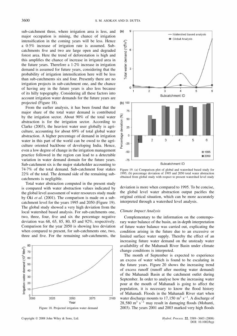
Total water abstraction computed in the present studyis compared with water abstraction values indicated bythe global level assessment of water resources study madeby Oki et al. (2001). The comparison is made on a sub-catchment level for the years 1995 and 2050 (Figure 19).The global study showed a very high deviation from thelocal watershed based analysis. For sub-catchments one,two, three, four, five and six the percentage negativedeviation was 68, 65, 85, 80, 85 and 92%, respectively.Comparison for the year 2050 is showing less deviationwhen compared to present, for sub-catchments one, two,three and five. For the remaining sub-catchments, the

Figure 18. Projected irrigation water demand

Figure 19. (a) Comparison plot of global and watershed based study for1995; (b) percentage deviation of 1995 and 2050 total water abstractionobtained from global study with respect to present watershed level study

deviation is more when compared to 1995. To be concise,the global level water abstraction output pacifies theoriginal critical situation, which can be more accuratelyinterpreted through a watershed level analysis.

Climate Impact Analysis

Complementary to the information on the contempo-rary water balance of the basin, an in-depth interpretationof future water balance was carried out, explicating thecondition arising in the future due to an excessive orlimited surface water supply. Thereby the effect of anincreasing future water demand on the unsteady wateravailability of the Mahanadi River Basin under climatechange conditions is interpreted.

The month of September is expected to experiencean excess of water which is found to be escalating inthe future years. Figure 20 shows the increasing trendof excess runoff (runoff after meeting water demand)of the Mahanadi Basin at the catchment outlet duringSeptember. In order to analyse how the increasing waterpour at the mouth of Mahanadi is going to affect thepopulation, it is necessary to know the flood historyof Mahanadi. Floods in the Mahanadi River start whenwater discharge mounts to 17,150 m3 s�1. A discharge of28,580 m3 s�1 may result in damaging floods (Mohanti,2003). The years 2001 and 2003 marked very high floods



Figure 20. Plot of excess discharge of the Mahanadi Basin

in the Mahanadi River. The highest discharge recordedwas 40,868 m3 s�1. The extent of damage brought aboutby 2001 flood is tabulated in Table VI (UNDMT, 2001).It explains the degree of catastrophe experienced bythe population because of a destructive flood whichlasted only for a couple of days. The findings of thecurrent study are pointing towards the future possibilityof floods during the month of September with an evenhigher magnitude because of climatic change. Therefore,apposite flood management measures have to be takenwell in advance to save the population, especially thosethriving in the delta region. Looking at the contemporaryand successive water stress factor for the MahanadiBasin, it is found that sub-catchment one shows thelargest amount of shortage of 467 MCM for 2000.All other sub-catchments show water shortage volumeranging from 56 to 160 MCM (Figure 21). Figure 22shows the percentage increase in water demand andthe percentage decrease in water availability for thefuture years. It can be observed from Figure 22 that thepercentage decrease in water availability is maximumduring the period 2050–2075. However, the percentageincrease in water demand shows a negative trend duringthe same period. This in effect pacifies the intensity ofwater stress in the basin during the same period. All thesub-catchments are growing towards a high degree ofscarcity during the period from 2000 to 2050. However,beyond 2050 the intensity of scarcity is seen alleviated.The main reason behind this is the reduction in waterdemand beyond 2050 owing to the zero growth ratein population assumed to be attained according to theplanning propaganda of the state. Figure 23 shows thewater stress projected for the year 2100 and the per capitawater availability under this projected stress conditions.From the per capita water availability illustrated inFigure 23, it is clear that all the sub-catchments are underwater stress. Within this stress realm, sub-catchmentsone and three can be considered as under peak stress,because the per capita water availability for these sub-catchments is even less than 5% of the maximum percapita water availability with respect to the whole basin.Sub-catchments four, five and two can be consideredas under medium stress since the per capita wateravailability in these sub-catchments is varying from 10

to 30% of the maximum value. Sub-catchment six, whichis having the maximum per capita water availability of4Ð41 litres per day, can be considered as under low stress.

In recent years, the Mahanadi River Basin is experi-encing drought in the same region, which was floodedat some point of time. It has already been mentionedthat this river basin experienced the peak flood in theyear 2001. The basin also experienced the worst hitdrought also in the same year. Western Orissa districtswere mainly affected. Media reported about 16 starvationdeaths. Migration of people from the drought strickenareas to the neighbouring states of Madhya Pradesh,Maharashtra, and Gujarat was also observed during thisperiod (UN, 2001). The present study predicts an increas-ing trend of water scarcity in the dry season all through

Table VI. Flood damage tabulated for 2001 flood

Sl no. Particular Loss

1 Death toll 392 Flood affected population 5Ð978 million3 Number of districts affected 244 Number of blocks affected 1495 Number of panchayats affected 15966 Number of villages affected 91517 Number of houses damaged 27,6328 Crop loss 0Ð00375 million km2

9 Crop loss estimated US$5 million

Figure 21. Water shortage for the year 2000

Figure 22. Percentage variation in water availability and demand



Figure 23. Sub-catchment level projected water shortage for 2100

the coming decades. This necessitates appropriate waterharvesting techniques during the peak season to savewater, which would have otherwise be lost in the sea.

CONCLUSIONS

Climate change has the potential to alter the adequacy andfrequency of precipitation leading to a sporadic hydro-logic cycle, the climax of which can be reflected in thewater supply and demand aspects. The present study pro-vides an assessment of the impact of climate change onwater resources of the Mahanadi River Basin throughoutthe twenty-first century. A DHM driven by GCM outputwas used in this study to forecast present and future wateravailability. The future water availability forecast indi-cated an escalating trend in river runoff thereby alarm-ing flood in this highly climatically vulnerable basin forthe month of September. The outcomes of the analysisfor the month of April however indicate an acceleratingwater scarcity in the future. The finding of the analy-sis on present scenario water demand indicates a highwater abstraction by the irrigation sector. Among thesix sub-catchments, sub-catchment six shows the peakwater demand. The future water demand is projectedfrom the contemporary state using appropriate projectiontechniques, and it is observed that the demand is increas-ing until 2050, beyond which the demand will decreaseowing to the assumed regulation of population. Regionof Mahanadi under peak stress is predicted and per capitawater availability under stress condition is estimated. Thisstudy hence reveals the vulnerability of the MahanadiRiver Basin to climate change. The output from this studycan be considered as a guideline for the policy-makers toplan and prepare for future floods and droughts.

The study has presented a framework of comprehen-sive analysis of impacts of climate change in waterresources at river basin scale such that outcomes of thestudy can be directly utilized for decision-making pro-cess. The large scale heterogeneity in water resourcesin countries like India underlies the importance of sub-basin scale comprehensive understanding of impacts ofclimate change. The generic methodology used in thestudy can be transferred to any other river basins foranalysing impacts of climate change in water resourcestowards adaptive management.

The accuracy of future water availability forecastdepends on the GCM projections used. The major prob-lem in applying GCM projections to finer area assessmentis that the coarse resolution of the data may not realisti-cally represent the orography and land surface processesleading to deviation of observed and modelled rain-fall pattern. Hence appropriate downscaling techniquesneed to be followed. This study looked into the quan-tity aspects of surface water resources under climaticvariation. The conjunctive use of surface and groundwa-ter resources with adequate allowance for environmentalshould be included for enhancement of the findings forwater resources management.

REFERENCES

Amarasinghe U. 2003. Spatial variation in water supply and demandacross the River Basins of India, Draft Research Report, IWMI,Colombo, Sri Lanka. Available at http://www.icid.org/report upalinov03.pdf.

Arnell NW. 1999. Climate change and global water resources. GlobalEnvironmental Change S31–S49.

Arnell NW. 2000. Global climate change and water resources: to 2025and beyond. In An ODI (The Overseas Development Institute)-SOAS(The School of Oriental and African Studies) Meeting Series Leading



up to the Second World Water Forum and Ministerial Conference,Overseas Development Institute, February 2000; 17–22.

Arnell NW. 2004. Climate change and global water resources: SRESemissions and socio-economic scenarios. Global EnvironmentalChange 14: 31–52.

Alcamo J, Doll P, Kaspar F, Siebert S. 1997. Global Change and GlobalScenarios of Water Use and Availability: An Application of Water GAP1Ð0 . Center for Environmental Systems Research (CESR), Universityof Kassel: Kassel.

Arora VK, Boer GJ. 2001. Effects of simulated climate change on thehydrology of major river basins. Journal of Geophysical Research106(D4): 3335–3348.

Asokan SM. 2005. Water resources analysis under projected climateconditions in the Mahanadi River Basin, India. MEng thesis, No.WM-04-13, Asian Institute of Technology, Thailand; 87 pp.

Bear J, Verruijt A (ed.). 1987. Modeling Ground Water Flow andPollution. D. Reidel Publishing Company: Dordrecht.

Bhuiyan JAB. 2005. Assessment of the economic impacts of floods underclimate change conditions in a coastal city in Bangladesh. MEng thesis,No. WM-04-12, Asian Institute of Technology, Thailand; 113 pp.

CSE. 2003. Climate Change and Orissa, Factsheet, Global EnvironmentalNegotiations. Available at http://www.cseindia.org/programme/geg/pdf/orissa.pdf (accessed September 15, 2005).

Clarke R. 2003. Water Crisis? OECD Observer. Available athttp://www.oecdobserver.org/news/fullstory.php/aid/935/Watercrisis .html (accessed September 10, 2005).

Dickinson R, Sellers AH, Kennedy PJ. 1993. Biosphere AtmosphereTransfer Schemes (BATS) as coupled to the Community Climate Model ,NCAR Technical Note, NCAR/TN-383CSTR, National Center forAtmospheric Research: Boulder, CO.

Dutta D, Herath S, Musiake K. 2000. Flood inundation simulation ina river basin using a physically based distributed hydrologic model.Hydrological Processes 14: 497–519.

Food and Agriculture Organization of the United Nations (FAO)Soil MAP. 2003. Available at http://www.fao.org/ag/agl/agll/wrb/mapindex.stm (accessed October 28, 2005).

Flato GM, Boer GJ, Lee WG, McFarlane NA, Ramsden D, Reader MC,Weaver AJ. 2000. The Canadian centre for climate modeling andanalysis global coupled model and its climate. Climate Dynamics 16:451–467.

Frederick KD, Major DC, Stakhiv EZ. (eds). 1997. Climate Change andWater Resources Planning Criteria. Kluwer Academic: Norwell, MA.

Ghosh S, Mujumdar PP. 2006. Future rainfall scenario over Orissa withGCM projections by statistical downscaling, Current Science 90(3):396–404.

Gleick PH. 1997. Water 2050: Moving Toward a Sustainable Visionfor the Earth’s Fresh Water . Working Paper of the Pacific Institutefor Studies in Development, Environment, and Security, Oakland,California. Prepared for the Comprehensive Freshwater Assessment forthe United Nations General Assembly and the Stockholm EnvironmentInstitute, Stockholm, Sweden.

Gleick PH. 2000. Water: The Potential Consequences of ClimateVariability and Change for the Water Resources of the United States . USGlobal Change Program. Pacific Institute for Studies in Development,Environment, and Security: Oakland, CA.

Global Environment Outlook. 2000. Fresh water. UNEP, Thestate of the environment, Regional Synthesis. Available athttp://www.unep.org/geo2000/english/0046.htm (accessed October 12,2005).

Gosain AK, Rao S. 2003. Impacts of climate change on water sector. InClimate Change and India: Vulnerability Assessment and Adaptation ,Shukla PR, Sharma SK, Ravindranath NH, Garg A, Bhattachatya S(eds). Universities Press: Andhra Pradesh.

International Food Policy Research Institute (IFPRI). 2002. GlobalWater Outlook to 2025: Averting an Impending Crisis. Availableat http://www.ifpri.org/media/water countries.htm#india [January 152005].

Intergovernmental Panel on Climate Change (IPCC). 2001. ClimateChange 2001: Impacts, Adaptation and Vulnerability. Contribution ofWorking Group II to the Third Assessment Report of the IPCC.Cambridge University Press: Cambridge.

Isard W. 1960. Methods of Regional Analysis. In Population Projection,The MIT Press: Cambridge, MA; 5–33.

Jha R, Herath S, Musiake K. 1997. Development of IIS DistributedHydrological Model (IISDHM) and its application in Chao PhrayaRiver Basin, Thailand. Annual Journal of Hydraulic Engineering,JSCE , 41: 227–232.

Katz RW, Parlange MB. 1996. Mixtures of stochastic processes:application to statistical downscaling. Climate Research 7: 185–193.

Kay AL, Reynard NS. 2006. RCM rainfall for UK flood frequencyestimation. I. Method and validation. Journal of Hydrology 318(1–4):151–162.

Kristensen K, Jensen S. 1975. A model for estimating actual evapo-transpiration from potential evapotranspiration. Nordic Hydrology 6:70–88.

Lal M, Cubasch U, Voss R, Waszkewitz J. 1995. Effect of transientincrease in greenhouse gases and sulphate aerosols on monsoon.Current Science 69(9): 752–763.

Lettenmaier DP, Wood AW, Palmer RN, Wood EF, Stakhiv EZ. 1999.Water resources implications of global warming: A U.S. regionalperspective. Climate Change 43: 537–579.

Lonergan S. 1998. Climate warming and India. In Measuring the Impactof Climate Change on Agriculture, Dinar A (ed.), World Bank TechnicalPaper No. 402. The World Bank: Washington, DC.

Marsily CD. 1986. Quantitative Hydrogeology , Academic Press: NewYork.

Mirza MMQ, Ahmed AU. 2003. Climate changes and water resourcesin South Asia: Vulnerabilities and coping mechanisms—a synthesis.In Climate Change and Water Resources in South Asia, Muhammed A(ed.). Asian-Pacific Network (APN): Kobe.

Mohanti M. 2003. Mahanadi river delta, east coast of India:an overview on evolution and dynamic processes. Available athttp://www.megadelta.ecnu.edu.cn/main/upload/mahanadi.pdf(accessed September 12, 2005).

Nguyen VTV. 2005. Downscaling methods for evaluating the impacts ofclimate change and variability on hydrological regime at basin scale. InProceedings of the International Symposium on Role of Water Sciencesin Transboundary River Basin Management, Thailand ; 1–8.

Orissa Census. 2001. Primary Census Abstract, Census of India . Officeof the Registrar General: New Dehli.

Oki T. 2003. Global water resources assessment under climatic changein 2050 using TRIP. Water resources systems—water availabilityand global change. In Proceedings of Symposium HS02a held duringIUGG2003 at Sapporo, IAHS Publication No. 280. IAHS Press:Wallingford.

Oki T, Agata Y, Kanae S, Saruhashi T, Yang D, Musiake K. 2001.Global assessment of current water resources using Total RunoffIntegrating Pathways. Hydrological Sciences 46(6): 983–995.

Pant GB, Kumar KR. 1997. Climates of South Asia. John Wiley and Sons:Singapore; 18.

Prudhomme C, Reynard M, and Crooks S. 2002. Downscaling of globalclimate models for flood frequency analysis: where are we now?Hydrological Processes 16: 1137–1150.

Shiklomanov IA. 1993. World fresh water resources. In Water in Crisis: AGuide to the World’s Fresh Water Resources . Gleick PH (ed.). OxfordUniversity Press: New York.

Shiklomanov IA. 1998. Assessment of water resources and wateravailability in the world . Report for the Comprehensive Assessment ofthe Freshwater Resources of the World, United Nations. Data archiveon CD-ROM from the State Hydrological Institute, St Petersburg,Russia.

Thomas R. (ed.). 1973. Ground Water Models . FAO: Rome.UNDMT Situation Report. 2001. Orissa Floods 2001. Avail-

able at http://www.un.org.in/dmt/orissa/072001flood/sitreps/ (accessedSeptember 5, 2005).

United Nations (UN). 2001. Situation report on Orissa drought 2001.Available at http://www.un.org.in/dmt/orissa/ (accessed August 30,2005).

US Geological Survey (USGS). 2003. Land processes distributed activearchive centre. Available at http://edcdaac.usgs.gov/gtopo30/hydro/asia.asp (accessed September 30, 2005).

van Dam JC. (ed.) 1999. Impacts of Climate Change and ClimateVariability on Hydrologic Regimes . Cambridge University Press: NewYork.

Vorosmarty CJ, Green P, Salisbury J, Lammers RB. 2000. Global waterresources: vulnerability from climate change and population growth.Science 289: 284–288.

Wilby RL, Hay LE, Leavesley GH. 1999. A comparison of downscaledand raw GCM output: implications for climate change scenarios in theSan Juan River Basin, Colorado. Journal of Hydrology 225: 178–191.

World Health Organization (WHO). 2004. Minimum Water QuantityNeeded for Domestic Uses . WHO Regional Office for South-east Asia:New Dehli.

World Resources Institute. 1990. World Resources 1990–91 . OxfordUniversity Press: New York.


1_asokan and dutta_hp_2008

Documents

climate change conditions

future water demand

projected water demand

water demand estimation

peak water demand

climate change leads

climate change ipcc

climate change manifests