1998 technical noise supplement
TRANSCRIPT


TECHNICAL NOISE SUPPLEMENTOctober 1998
ACKNOWLEDGEMENT
The Technical Noise Supplement evolved from a 1991 draft document titled Noise Technical AnalysisNotes (NoTANs) prepared by the former Division of New Technology and Research (TransLab). DickWood, a TransLab staff member, and I were the authors of the 1991 draft NoTANs. For various reasonsNoTANs was never finalized. However, I edited, re-wrote, and revised original contents of the draftNoTANs and incorporated these with new information in this Technical Noise Supplement (TeNS). DickWood's early contributions to NoTANs were extremely valuable to the development of TeNS, and Iwant to sincerely thank him for assisting me in the effort leading to the final completion of TeNS.
I also owe a great debt of gratitude to:
Professor Dean Karnopp of the University of California at Davis, Department of Mechanical andAeronautical Engineering, for his constructive review and contributions to TeNS.
●
Joya Gilster, Civil Engineering Student, for her detailed technical review of TeNS.●
Keith Jones for his constructive review and comments, and for believing in TeNS and me. Hisundying support and enthusiasm for this project is directly responsible for the emergence of TeNSfrom NoTAN. Without his support TeNS would not have succeeded.
●
To all mentioned above, I sincerely appreciate your help.
Environmental Engineering-Noise, Air Quality, and Hazardous Waste Management Office,October 1998
http://www.dot.ca.gov/hq/Environmental/offdocs/hazdocs/tens/ack.htm [1/19/2000 3:46:31 PM]

TECHNICAL NOISE SUPPLEMENTOctober 1998
N-1
N-1000 INTRODUCTION AND OVERVIEWN-1100 INTRODUCTIONThe purpose of this Technical Noise Supplement (TeNS) is to provide technical background
information on transportation-related noise in general and highway traffic noise in
particular. It is designed to elaborate on technical concepts and procedures referred to in
the Caltrans Traffic Noise Analysis Protocol (the Protocol). The contents of this Supplement
are for informational purposes only and unless specifically referred to as such in the
Protocol they are not official policy, standard or regulation. The procedures recommended
in TeNS are in conformance with “industry standards”.
This document can also be used as a “stand alone” document for training purposes, or as a
reference for technical concepts, methodology, and terminology needed to acquire a basic
understanding of transportation noise with emphasis on highway traffic noise.
N-1200 OVERVIEWTeNS consists of nine sections, numbered N-1000 through N-9000. With the exception of
N-1000 (this section), each section covers a specific subject of highway noise. A brief
description of the subjects follows.
• N-2000, BASICS OF HIGHWAY NOISE covers the physics of sound as it pertains to
characteristics and propagation of highway noise, the effects of noise on humans,
and ways of describing noise.
• N-3000, MEASUREMENTS AND INSTRUMENTATION covers the “why, where, when,
and how” of noise measurements, and briefly discusses various noise measuring
instruments and operating procedures.
• N-4000, SCREENING PROCEDURE was developed to aid in determining whether or
not a highway project has the potential to cause a traffic noise impact. If the project
passes the screening procedure, prudent engineering judgment should still be
exercised to determine if a detailed analysis is warranted.
• N-5000, DETAILED ANALYSIS – TRAFFIC NOISE IMPACTS gives guidance for
studying those projects failing the screening procedure, projects that are
controversial, sensitive, or projects where the net effects of topography and shielding
are complex and ambiguous.

TECHNICAL NOISE SUPPLEMENTOctober 1998
N-2
• N-6000, DETAILED ANALYSIS - NOISE BARRIER DESIGN CONSIDERATIONS outlines
the major aspects that affect the acoustical design of noise barriers. These include
the dimensions, location, material, and optimization of noise barriers; the acoustical
design of overlapping noise barriers (to provide maintenance access to areas behind
barriers) and drainage openings in noise barriers. It also points out some pitfalls
and cautions.
• N-7000, NOISE STUDY REPORTS discusses the contents of noise study reports.
• N-8000, SPECIAL CONSIDERATIONS covers some special controversial issues that
frequently arise, such as reflective noise, the effects of noise barriers on distant
receivers, and shielding provided by freeway landscaping.
• N-9000, GLOSSARY provides terminology and definitions common in transportation
noise.
In addition to the above sections the BIBLIOGRAPHY provides a listing of literature used
as a source of information in TeNS.

3
N-2000 BASICS OF HIGHWAY NOISEThe following sections introduce the fundamentals of sound and provide sufficient detail for
the reader to understand the terminology and basic factors involved in highway traffic noise
prediction and analysis. Those who are actively involved in noise analysis are encouraged
to seek out more detailed textbooks and reference books in order to acquire a deeper
understanding of the subject.
N-2100 PHYSICS OF SOUND
N-2110 Sound, Noise, Acoustics
Sound is a vibratory disturbance created by a moving or vibrating source, in the pressure
and density of a gaseous, liquid medium or in the elastic strain of a solid which is capable
of being detected by the hearing organs. Sound may be thought of as mechanical energy of
a vibrating object transmitted by pressure waves through a medium to human (or animal)
ears. The medium of main concern is air. In absence of any other qualifying statements,
sound will be considered airborne sound, as opposed to, for example, structureborne or
earthborne sound.
Noise is defined as (airborne) sound that is loud, unpleasant, unexpected or undesired, and
may therefore be classified as a more specific group of sounds. Perceptions of sound and
noise are highly subjective: one person's music is another's headache. The two terms are
often used synonymously, although few would call the sound that emanates from a
highway anything but noise.
Sound (and noise) is actually a process that consists of three components: 1) the sound
source, 2) the sound path, and 3) the sound receiver. All three components must be present
for sound to exist. Without a source to produce sound, there obviously is no sound.
Likewise, without a medium to transmit sound pressure waves there is also no sound. And
finally, sound must be received, i.e. a hearing organ, sensor, or object must be present to
perceive, register, or be affected by sound or noise. In most situations, there are many
different sound sources, paths, and receivers, instead of just one of each.
Acoustics is the field of science that deals with the production, propagation, reception,
effects, and control of sound. The field is very broad, and transportation related noise and
its abatement covers just a small, specialized part of acoustics.

4
N-2120 Speed of Sound
When the surface of an object vibrates in air, it compresses a layer of air as the surface
moves outward, and produces a rarefied zone as the surface moves inward. This results in
a series of high and low air pressures waves (relative to the steady ambient atmospheric
pressure) alternating in sympathy with the vibrations. These pressure waves - not the air
itself - move away from the source at the speed of sound, or approximately 343 m/s (1126
ft/sec) in air of 20o C. The speed of sound can be calculated from the following formula:
c = 1 401.Pρ
�
��
�
�� (eq. N-2120.1)
Where:
c = Speed of Sound at a given temperature, in meters per second (m/s)
P = Air pressure in Newtons per Square Meter (N/m2) or Pascals (Pa)
ρ = Air density in kilograms of mass per cubic meter (Kg/m3)
1.401 = the ratio of the specific heat of air under constant pressure to that of air in
a constant volume.
For a given air temperature and relative humidity, the ratio P/ρ tends to remain constant in
the atmosphere, because the density of air will reduce or increase proportionally with
changes in pressure. Thus the speed of sound in our atmosphere is independent of air
pressure. However, when air temperature changes, only ρ changes, while P does not. The
speed of sound is therefore temperature dependent, and also somewhat humidity
dependent since humidity affects the density of air. The effects of the latter with regards to
the speed of sound, however, can be ignored for our purposes. The fact that speed of
sound changes with altitude, has nothing to do with the change in air pressure, and is only
caused by the change in temperature.
For dry air of 0o Celsius, ρ = 1.2929 Kg/m3. At a standard air pressure of 760 mm Hg, the
pressure in Pa = 101,329 Pa. Using eq. N-2120.1, the speed of sound for standard
pressure and temperature can be calculated:
( )( )..
1 40 11 01 3 291 2 92 9
= 331.4 m/sec, or 1087.3 ft/sec. From this base value, the variation
with temperature is described by the following equations:
Metric Units (m/s): c = 331.4 1 +Tc
273.2(eq. N-2120.2)

5
English Units (ft/sec): c = 1051.3 1 +Tf
459.7(eq. N-2120.3)
Where:
c = speed of sound in m/s (metric) or ft/sec (English)
Tc = Temperature in degrees Celcius (include minus sign for below zero)
Tf = Temperature in degrees Fahrenheit (include minus sign for below zero)
The above equations show that the speed of sound increases/decreases as the air
temperature increases/decreases. This phenomenon plays an important role in the
atmospheric effects on noise propagation, specifically through the process of refraction,
which is discussed in section N-2143 (Meteorological Effects and Refraction).
N-2130 Sound Characteristics
In its most basic form, a continuous sound can be described by its frequency or wavelength
(pitch) and its amplitude (loudness).
N-2131 Frequency, Wavelength, Hertz
For a given single pitch of sound, the sound pressure waves are characterized by a
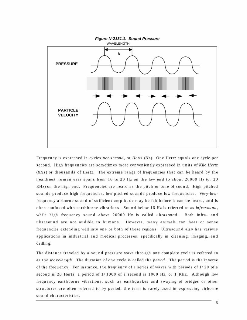
sinusoidal periodic (recurring with regular intervals) wave as shown in Figure N-2131.1.
The upper curve shows how sound pressure varies above and below the ambient
atmospheric pressure with distance at any given time. The lower curve shows how particle
velocity varies above zero (molecules moving right) and below zero (molecules moving left).
Particle velocity describes the motion of the air molecules in response to the pressure
waves. It does not refer to the velocity of the waves, otherwise known as the speed of
sound. The distance (λ) between crests of both curves is the wavelength of the sound.
The number of times per second that the wave passes from a period of compression
through a period of rarefaction and starts another period of compression, is referred to as
the frequency of the wave (see Figure N-2131.2).
6
Figure N-2131.1. Sound Pressure
Frequency is expressed in cycles per second, or Hertz (Hz). One Hertz equals one cycle per
second. High frequencies are sometimes more conveniently expressed in units of Kilo Hertz
(KHz) or thousands of Hertz. The extreme range of frequencies that can be heard by the
healthiest human ears spans from 16 to 20 Hz on the low end to about 20000 Hz (or 20
KHz) on the high end. Frequencies are heard as the pitch or tone of sound. High pitched
sounds produce high frequencies, low pitched sounds produce low frequencies. Very-low-
frequency airborne sound of sufficient amplitude may be felt before it can be heard, and is
often confused with earthborne vibrations. Sound below 16 Hz is referred to as infrasound,
while high frequency sound above 20000 Hz is called ultrasound. Both infra- and
ultrasound are not audible to humans. However, many animals can hear or sense
frequencies extending well into one or both of these regions. Ultrasound also has various
applications in industrial and medical processes, specifically in cleaning, imaging, and
drilling.
The distance traveled by a sound pressure wave through one complete cycle is referred to
as the wavelength. The duration of one cycle is called the period. The period is the inverse
of the frequency. For instance, the frequency of a series of waves with periods of 1/20 of a
second is 20 Hertz; a period of 1/1000 of a second is 1000 Hz, or 1 KHz. Although low
frequency earthborne vibrations, such as earthquakes and swaying of bridges or other
structures are often referred to by period, the term is rarely used in expressing airborne
sound characteristics.
PRESSURE
WAVELENGTH
λλλλ
PARTICLEVELOCITY
7
Figure N-2131.2 shows that as the frequency of sound pressure waves increases, their
wavelength shortens, and vice versa. The relationship between frequency and wavelength
is linked by the speed of sound, as shown in the following equations:
λλλλ = cf (eq. N-2131.1)
Also: f = cλ
(eq. N-2131.2)
and: c = fλλλλ (eq. N-2131.3)
Where:
λ = Wavelength (m or ft)
c = Speed of Sound (343.3 m/s, or 1126.5 ft/sec at 20o C, or 68o F)
f = Frequency (Hertz)
In the above equations, care must be taken to use the same units (distance units in either
meters or feet, and time units in seconds) for wavelength and speed of sound. Although the
speed of sound is usually thought of as a constant, we have already seen that it actually
varies with temperature. The above mathematical relationships hold true for any value of
the speed of sound. Frequency is normally generated by mechanical processes at the
source (wheel rotation, or back and forth movement of pistons, to name a few), and is
Figure N-2131.2 - Frequency and Wavelengthλλλλ
Wavelength, λλλλ
Short Wavelength, High Frequency
Long Wavelength, Low Frequency
8
therefore not affected by air temperature. As a result, wavelength usually varies inversely
with the speed of sound as the latter varies with temperature.
The relationships between frequency, wavelength and speed of sound can easily be
visualized by using the analogy of a train traveling at a given constant speed. Individual
boxcars can be thought of as the sound pressure waves. The speed of the train (and the
individual boxcars) is analagous to the speed of sound, while the length of each boxcar is
the wavelength. The number of boxcars passing a stationary observer each second depict
the frequency (f). If the value of the latter is 2, and the speed of the train (c) is 108 km/hr
(or 30 m/s), the length of each boxcar (λ) must be: c/f = 30/2 = 15m.
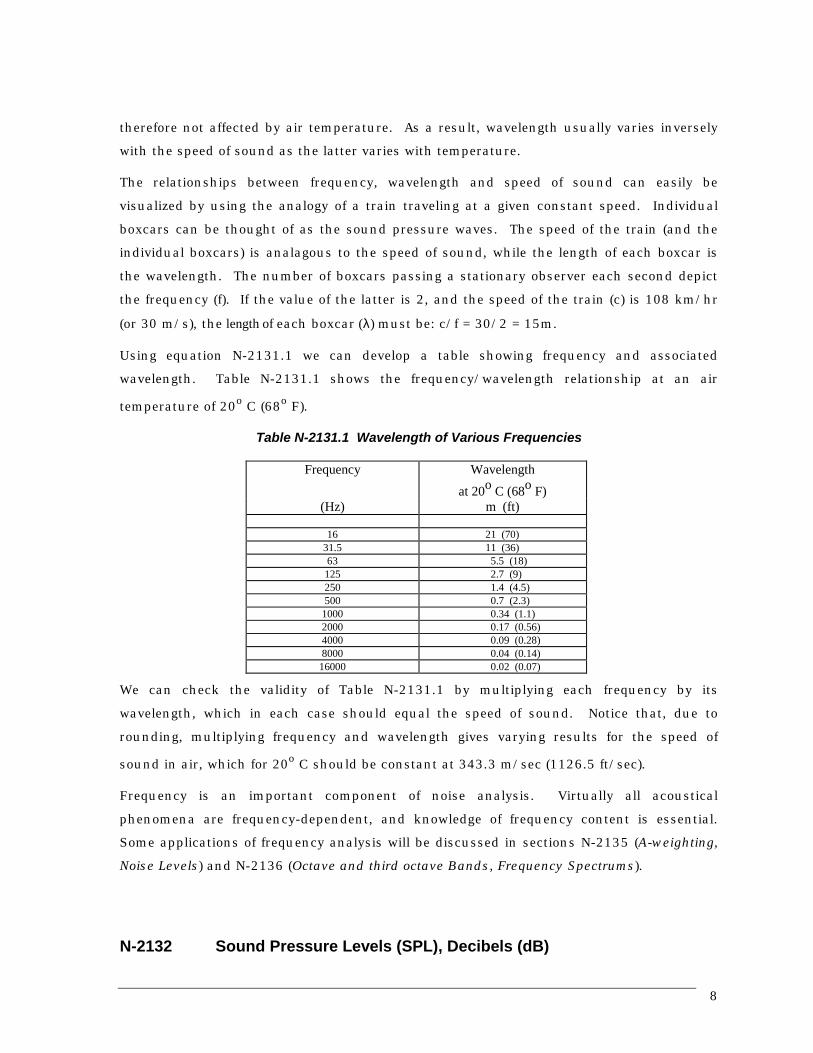
Using equation N-2131.1 we can develop a table showing frequency and associated
wavelength. Table N-2131.1 shows the frequency/wavelength relationship at an air
temperature of 20o C (68o F).
Table N-2131.1 Wavelength of Various Frequencies
Frequency Wavelength
at 20o C (68o F)(Hz) m (ft)
16 21 (70)31.5 11 (36)63 5.5 (18)125 2.7 (9)250 1.4 (4.5)500 0.7 (2.3)
1000 0.34 (1.1)2000 0.17 (0.56)4000 0.09 (0.28)8000 0.04 (0.14)
16000 0.02 (0.07)
We can check the validity of Table N-2131.1 by multiplying each frequency by its
wavelength, which in each case should equal the speed of sound. Notice that, due to
rounding, multiplying frequency and wavelength gives varying results for the speed of
sound in air, which for 20o C should be constant at 343.3 m/sec (1126.5 ft/sec).
Frequency is an important component of noise analysis. Virtually all acoustical
phenomena are frequency-dependent, and knowledge of frequency content is essential.
Some applications of frequency analysis will be discussed in sections N-2135 (A-weighting,
Noise Levels) and N-2136 (Octave and third octave Bands, Frequency Spectrums).
N-2132 Sound Pressure Levels (SPL), Decibels (dB)

9
Referring back to Figure N-2131.1, we remember that the pressures of sound waves
continuously changes with time or distance, and within certain ranges. The ranges of these
pressure fluctuations (actually deviations from the ambient air pressure) are called the
amplitude of the pressure waves. Whereas the frequency of the sound waves is reponsible
for the pitch or tone of a sound, the amplitude determines the loudness of the sound.
Loudness of sound increases and decreases with the amplitude.
Sound pressures can be measured in units of micro Newtons per square meter (µN/m2)
called micro Pascals (µPa). 1 µPa is approximately one-hundredbillionth of the normal
atmospheric pressure. The pressure of a very loud sound may be 200,000,000 µPa, or
10,000,000 times the pressure of the weakest audible sound (20 µPa). Expressing sound
levels in terms of µPa would be very cumbersome, however, because of this wide range. For
this reason, sound pressure levels (SPL) are described in logarithmic units of ratios of actual
sound pressures to a reference pressure squared. These units are called bels, named after
Alexander G. Bell. In order to provide a finer resolution, a bel is subdivided into 10 decibels
(deci or tenth of a bel), abbreviated dB. In its simplest form, sound pressure level in
decibels is expressed by the term:
Sound Pressure Level (SPL) = 10 Log10 ( 1
0
pp )2
dB (eq. N-2132.1)
Where:
P1 is sound pressure
P0 is a reference pressure, standardized as 20 µPa
The standardized reference pressure, P0, of 20 µPa, is the absolute threshold of hearing in
healthy young adults. When the actual sound pressure level is equal to the reference
pressure, the expression:
10Log10 ( 1
0
pp )2
= 10Log10 (1) = 0 dB
Note that 0 dB is not the absence of any sound pressure. Instead, it is an extreme value
that only those with the most sensitive ears can detect. Thus, it is possible to refer to
sounds as less than 0 dB (negative dB), for sound pressures that are weaker than the
threshold of human hearing. For the majority of people, the threshold of hearing is higher
than 0 dB, probably closer to 10 dB.

10
N-2133 Root Mean Square (Rms), Relative Energy
Figure N-2131.1 depicted a sinusoidal curve of pressure waves. The values of the pressure
waves were constantly changing, increasing to a maximum value above normal air pressure
then deceasing to a minimum value below normal air pressure, in a repetitive fashion. This
sinusoidal curve is associated with a single frequency sound, also called a pure tone. Each
successive sound pressure wave has the same characteristics as the previous wave. The
amplitude characteristics of such a series of simple waves can then be described in various
ways, all of which are simply related to each other. The two most common ways to describe
the amplitude of the waves is in terms of the peak sound pressure level (SPL) and the root
mean square (r.m.s.) SPL.
The peak SPL simply uses the maximum or peak amplitude (pressure deviation) for the
value of P1 in equation N-2132.1. The peak SPL therefore only uses one value (the absolute
value of the peak pressure deviation) of the continuously changing amplitudes. The r.m.s.
value of the wave amplitudes (pressure deviations) uses all the positive and negative
instantaneous amplitudes, not just the peaks. It is derived by squaring the positive and
negative instantaneous pressure deviations, adding these together and dividing the sum by
the number of pressure deviations. The result is called the mean square of the pressure
deviations, and taking the square root of this mean value is called the r.m.s. value. Figure
N-2133.1 shows the peak and r.m.s. relationship for a sinusoidal wave. The r.m.s. is 0.707
times the peak value.
Figure N-2133.1 Peak Vs. r.m.s. Sound Pressures
In terms of discrete samples of the pressure deviations the mathematical expression is:
r.m.s. value = √√√√(1����n(a1
2 + a22 + ..... an
2 )/n) (eq. N-2133.1)
Peak Negative Pressure
Peak Positive Pressure
r.m.s. PressurePRESSURE
0 Atmospheric Pressure
+
-
a1 a2 an

11
Sound pressures expressed in r.m.s. are proportional to the energy contents of the waves,
and are therefore the most important and often used measure of amplitude. Unless
otherwise mentioned, all SPL’s are expressed as r.m.s. values.
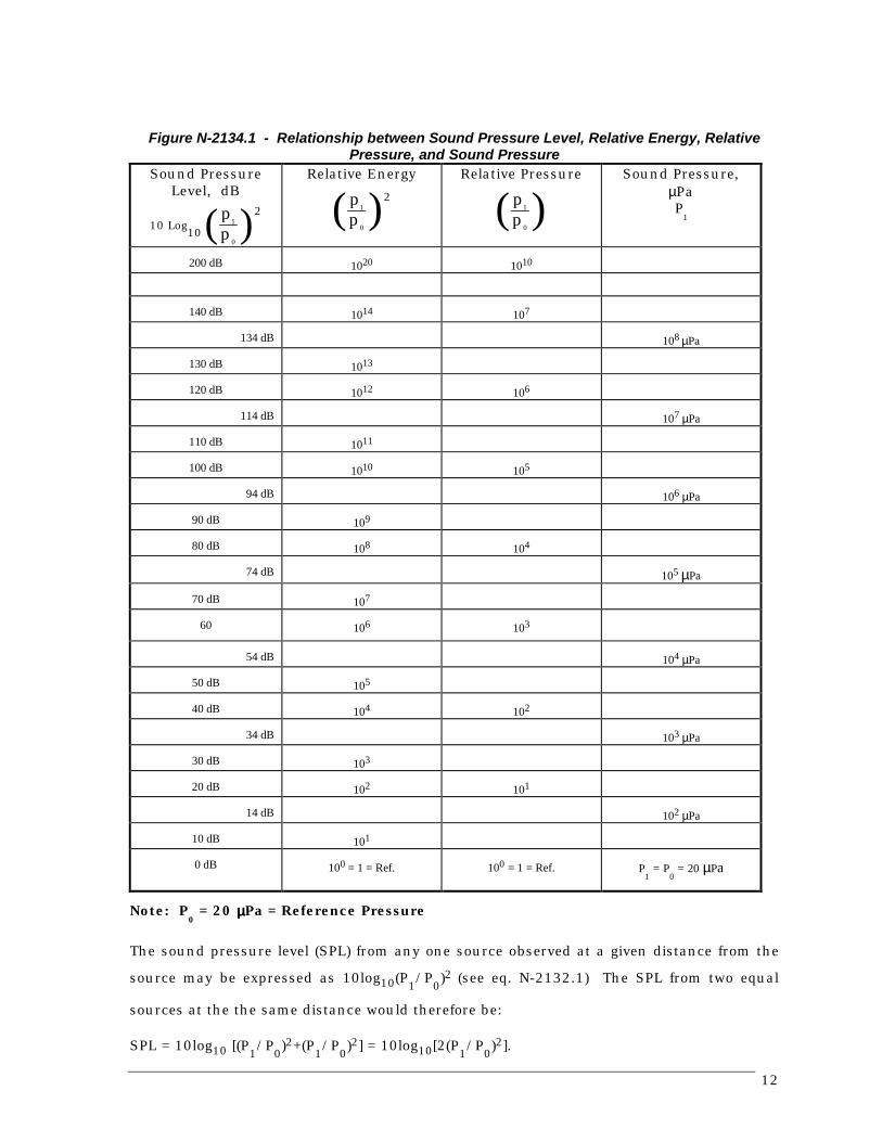
N-2134 Relationship Between Sound Pressure Level, Relative Energy,Relative Pressure, and Pressure
Table N-2134.1 shows the relationship between r.m.s. SPL’s, relative sound energy, relativesound pressure, and pressure.
Note that SPL’s, Relative Energy, and Relative Pressure are based on a Reference Pressure
of 20 µPa, and by definition all referenced to 0 dB. The Pressure values are the actual
r.m.s. pressure deviations from local ambient atmospheric pressure.
The most useful relationship is that of SPL (dB) and Relative Energy. Relative Energy is
unitless. Table N-2134.1 shows that for each 10 dB increase in SPL, the acoustic energy
increases 10-fold. For instance an SPL increase from 60 to 70 dB increases the energy 10
times. Acoustic energy can be thought of as the energy intensity (energy per unit area) of a
certain noise source, such as a heavy truck (HT), at a certain distance.
For example, if one HT passing by an observer at a given speed and distance produces an
SPL of 80 dBA, then the SPL of 10 HT’s identical to the single HT would be 90 dBA, if they
all could simultaneously occupy the same space, and travel at the same speed and distance
from the observer.
Since SPL = 10 Log10 (P1/P2)2, the acoustic energy is related to SPL as follows:
(P1/P2)2 = 10SPL/10 (eq. N-2134.1)
This relationship will be useful in understanding how to add and subtract SPL’s in the next
section.
N-2135 Adding and Subtracting Sound Pressure Levels (SPL’s)
Since decibels are logarithmic units, sound pressure levels cannot be added or subtracted
by ordinary arithmetic means. For example, if one automobile produces a SPL of 70 dB
when it passes an observer, two cars passing simultaneously would not produce 140 dB.
In fact, they would combine to produce 73 dB. This can be shown mathematically as
follows.
12
Figure N-2134.1 - Relationship between Sound Pressure Level, Relative Energy, RelativePressure, and Sound Pressure
Sound PressureLevel, dB
10 Log10 ( 1
0
pp )2
Relative Energy
( 1
0
pp )2
Relative Pressure
( 1
0
pp )
Sound Pressure,µPaP
1
200 dB 1020 1010
140 dB 1014 107
134 dB 108 µPa
130 dB 1013
120 dB 1012 106
114 dB 107 µPa
110 dB 1011
100 dB 1010 105
94 dB 106 µPa
90 dB 109
80 dB 108 104
74 dB 105 µPa
70 dB 107
60 106 103
54 dB 104 µPa
50 dB 105
40 dB 104 102
34 dB 103 µPa
30 dB 103
20 dB 102 101
14 dB 102 µPa
10 dB 101
0 dB 100 = 1 = Ref. 100 = 1 = Ref. P1 = P
0 = 20 µPa
Note: P0 = 20 µµµµPa = Reference Pressure
The sound pressure level (SPL) from any one source observed at a given distance from the
source may be expressed as 10log10(P1/P0)2 (see eq. N-2132.1) The SPL from two equal
sources at the the same distance would therefore be:
SPL = 10log10 [(P1/P0)2+(P1/P0)2] = 10log10[2(P1/P0)2].
13
This is can be simplified as 10log10(2)+10log10(P1/P0)2. Because the logarithm of 2 is
0.301, and 10 times that would be 3.01, the sound of two equal sources is 3 dB greater
than the sound level of one source. The total SPL of the two automobiles would therefore
be 70 + 3 = 73 dB.
Adding and Subtracting Equal SPL’s - The previous example of adding the noise levels of
two cars, may be expanded to any number of sources. The previous section discussed the
relationship between decibels and relative energy. The ratio (P1/P0)2 is the relative
(acoustic) energy portion of the expression SPL = 10log10(P1/P0)2, in this case the relative
acoustic energy of one source. This must immediately be qualified with the statement that
this is not the acoustic power output of the source. Instead, the expression is the relative
acoustic energy per unit area received by the observer. We may state that N identical
automobiles, or other noise sources, would yield an SPL of:
SPL(Total) = SPL(1) + 10log10(N) (eq. N-2135.1)
in which: SPL(1) = SPL of one source
N = number of identical sources to be added (must be ≥ 0)
Example: If one noise source produces 63 dB at a given distance, what would be the noise
level of 13 of the same sources combined at the same distance?
Solution: SPL(Total) = 63 + 10log10(13) = 63 + 11.1 = 74.1 dB
Equation N-2135.1 may also be rewritten as:
SPL(1) = SPL(Total) - 10log10(N) (eq. N-2135.2)
This form is useful for subtracting equal SPL’s.
Example: The SPL of 6 equal sources combined is 68 dB at a given distance. What is the
noise level produced by one source?
Solution: SPL(1) = 68 dB - 10log10(6) = 68 - 7.8 = 60 dB
In the above examples, adding equal sources actually constituted multiplying one source by
the number of sources. Conversely, subtracting equal sources was performed by dividing
the total. For the latter, we could have written eq. N-2135.1 as SPL(1) = SPL(Total) +
10log10(1/N). The logarithm of a fraction yields a negative result, so the answers would
have been the same.

14
The above excercises can be further expanded to include other useful applications in
highway noise. For instance, if one were to ask what the respective SPL increases would be
along a highway if existing traffic were doubled, tripled and quadrupled (assuming that
traffic mix, distribution, and speeds would not change), we could make a reasonable
prediction using equation N-2135.1. In this case N would be the existing traffic (N=1), N=2
would be doubling, N=3 tripling, and N=4 quadrupling the existing traffic. Since the
10log10(N) term in eq. N-2135.1 represents the increase in SPL, we can solve N for N=2,
N=3, and N=4. The results would respectively be: +3 dB, +4.8 dB, and +6 dB.
The question might also come up what the SPL decrease would be if the traffic would be
reduced by a factor of two, three, or four. In this case N = 1/2, N= 1/3, and N = 1/4,
respectively. Applying the 10log10(N) term for these values of N would result in -3 dB, -4.8
dB, and -6 dB, respectively.
The same problem may come up in a different form. For instance, if the traffic flow on a
given facility is presently 5000 vehicles per hour (vph) and the present SPL is 65 dB at a
given location next to the facility, what would the expected SPL be if future traffic increased
to 8000 vph? Solution: 65 + 10log10(8000/5000) = 65 + 2 = 67 dB.
The N value may thus represent an integer, a fraction, or a ratio. However, N must always
be greater than 0! Taking the logarithm of 0 or a negative value is not possible.
Adding and Subtracting Unequal Noise Levels. If noise sources are not equal, or if
equal noise sources are at different distances, the 10log10(N) term cannot be used. Instead,
the SPL’s have to be added or subtracted individually, using the SPL and relative energy
relationship in section N-2134 (eq. N-2134.1). If the number of SPL’s to be added is N, and
SPL(1), SPL(2), .....SPL(n) represent the 1st, 2nd, and nth SPL, respectively, the addition is
accomplished by:
SPL(Total) = 10log10[10SPL(1)/10+10SPL(2)/10 + ......... 10SPL(n)/10] (eq. N-2135.3).
The above equation is the general equation for adding SPL’s. The same equation may be
used for subtraction also (simply change the “+” to “-” for the term to be subtracted.
However, the result between the brackets must always be greater than 0!
For example, find the sum of the following sound levels: 82, 75, 88, 68, 79. Using
eq.2135.3, the total SPL is:
SPL = 10 Log10 (1068/10 + 1075/10 + 1079/10 + 1082/10 + 1088/10) = 89.6 dB

15
Adding SPL’s Using a Simple Table - When combining sound levels, the following table
may be used as an approximation.
Table N-2135.1 Decibel Addition
When Two Decibel Add This Amount
Values Differ By: to the Higher Value: Example:
0 or 1 dB 3 dB 70+69 = 73
2 or 3 dB 2 dB 74+71 = 76
4 to 9 dB 1 dB 66+60 = 67
10 dB or more 0 dB 65+55 = 65
This table yields results within ± 1 dB of the mathematically exact value and can easily be
memorized. The table can also be used to add more than two SPL’s. First, sort the list of
values, from lowest to highest. Then, starting with the lowest values, combine the first two,
add the result to the third value and continue until only the answer remains.
Example: find the sum of the sound levels used in the above example, using Table N-
2135.1. First, rank the values from low to high:
68 dB
75 dB
79 dB
82 dB
88 dB
?? dB Total
Using table 2135.1 add the first two noise levels. Then add the result to the next noise
level ............, etc.
a. 68 + 75 = 76,
b. 76 + 79 = 81,
c. 81 + 82 = 85,
d. 85 + 88 = 90 dB (For comparison, using eq.2135.3, the
total SPL was 89.6 dB).
Two decibel addition rules are important. First, when adding a noise level with another
approximately equal noise level, the total noise level rises 3 dB. For example doubling the
traffic on a highway would result in an increase of 3 dB. Conversely, reducing traffic by
one half, the noise level reduces by 3 dB. Second, when two noise levels are 10 dB or more
apart, the lower value does not contribute significantly (< 0.5 dB) to the total noise level.

16
For example, 60 + 70 dB ≈ 70 dB. The latter means that if a noise level measured from a
source is at least 70 dB, the ambient noise level without the target source must not be
more than 60 dB to avoid risking contamination.
N-2136 A-Weighting, Noise Levels
Sound pressure level alone is not a reliable indicator of loudness. The frequency or pitch of
a sound also has a substantial effect on how humans will respond. While the intensity
(energy per unit area) of the sound is a purely physical quantity, the loudness or human
response depends on the characteristics of the human ear.
Human hearing is limited not only to the range of audible frequencies, but also in the way
it perceives the sound pressure level in that range. In general, the healthy human ear is
most sensitive to sounds between 1,000 Hz - 5000 Hz, and perceives both higher and lower
frequency sounds of the same magnitude with less intensity. In order to approximate the
frequency response of the human ear, a series of sound pressure level adjustments is
usually applied to the sound measured by a sound level meter. The adjustments, or
weighting network, are frequency dependent.
The A-scale approximates the frequency response of the average young ear when listening
to most ordinary everyday sounds. When people make relative judgements of the loudness
or annoyance of a sound, their judgements correlate well with the A-scale sound levels of
those sounds. There are other weighting networks that have been devised to address high
noise levels or other special problems (B-scale, C-scale, D-scale etc.) but these scales are
rarely, if ever, used in conjunction with highway traffic noise. Noise levels for traffic noise
reports should be reported as dBA. In environmental noise studies A-weighted sound
pressure levels are commonly referred to as noise levels.
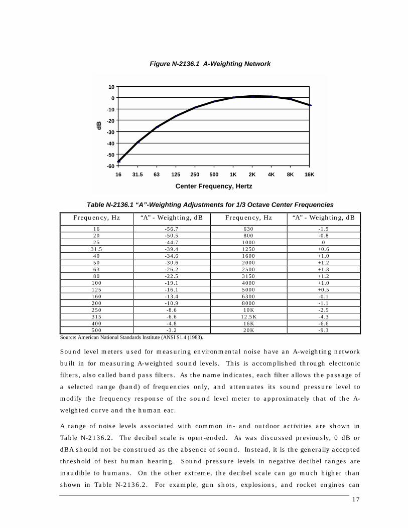
Figure N-2136.1 shows the A-scale weighting network that is normally used to approximate
human response. The zero dB line represents a reference line; the curve represents
frequency-dependent attenuations provided by the ear’s response. Table N-2136.1 shows
the standardized values (ANSI S1.4, 1983). The use of this weighting network is signified
by appending an "A" to the sound pressure level as dBA, or dB(A).
The A-weighted curve was developed from averaging the statistics of many psycho-acoustic
tests involving large groups of people with normal hearing in the age group of 18-25 years.
The internationally standardized curve is used world wide to address environmental noise
and is incorporated in virtually all environmental noise descriptors and standards. Section
N-2200 covers the most common of these, applicable to transportation noise.
17
Figure N-2136.1 A-Weighting Network
-60
-50
-40
-30
-20
-10
0
10
16 31.5 63 125 250 500 1K 2K 4K 8K 16K
Center Frequency, Hertz
Table N-2136.1 “A”-Weighting Adjustments for 1/3 Octave Center Frequencies
Frequency, Hz “A” - Weighting, dB Frequency, Hz “A” - Weighting, dB
16 -56.7 630 -1.920 -50.5 800 -0.825 -44.7 1000 0
31.5 -39.4 1250 +0.640 -34.6 1600 +1.050 -30.6 2000 +1.263 -26.2 2500 +1.380 -22.5 3150 +1.2100 -19.1 4000 +1.0125 -16.1 5000 +0.5160 -13.4 6300 -0.1200 -10.9 8000 -1.1250 -8.6 10K -2.5315 -6.6 12.5K -4.3400 -4.8 16K -6.6500 -3.2 20K -9.3
Source: American National Standards Institute (ANSI S1.4 (1983).
Sound level meters used for measuring environmental noise have an A-weighting network
built in for measuring A-weighted sound levels. This is accomplished through electronic
filters, also called band pass filters. As the name indicates, each filter allows the passage of
a selected range (band) of frequencies only, and attenuates its sound pressure level to
modify the frequency response of the sound level meter to approximately that of the A-
weighted curve and the human ear.
A range of noise levels associated with common in- and outdoor activities are shown in
Table N-2136.2. The decibel scale is open-ended. As was discussed previously, 0 dB or
dBA should not be construed as the absence of sound. Instead, it is the generally accepted
threshold of best human hearing. Sound pressure levels in negative decibel ranges are
inaudible to humans. On the other extreme, the decibel scale can go much higher than
shown in Table N-2136.2. For example, gun shots, explosions, and rocket engines can

18
reach 140 dBA or higher at close range. Noise levels approaching 140 dBA are nearing the
threshold of pain. Higher levels can inflict physical damage on such things as structural
members of air and spacecraft and related parts. Section N-2301 discusses the human
response to changes in noise levels.
Table N-2136.2 - Typical Noise Levels
COMMON OUTDOOR
ACTIVITIES
NOISE LEVEL
dBA
COMMON INDOOR
ACTIVITIES---110--- Rock Band
Jet Fly-over at 300 m (1000 ft)---100---
Gas Lawn Mower at 1 m (3 ft)---90---
Diesel Truck at 15 m (50 ft), Food Blender at 1 m (3 ft) at 80 km/hr (50 mph) ---80--- Garbage Disposal at 1 m (3 ft)Noisy Urban Area, DaytimeGas Lawn Mower, 30 m (100 ft) ---70--- Vacuum Cleaner at 3 m (10 ft)Commercial Area Normal Speech at 1 m (3 ft)Heavy Traffic at 90 m (300 ft) ---60---
Large Business OfficeQuiet Urban Daytime ---50--- Dishwasher Next Room
Quiet Urban Nighttime ---40--- Theater, Large ConferenceQuiet Suburban Nighttime Room (Background)
---30--- LibraryQuiet Rural Nighttime Bedroom at Night, Concert
---20--- Hall (Background)Broadcast/Recording Studio
---10---
Lowest Threshold of HumanHearing
---0--- Lowest Threshold of HumanHearing
N-2137 Octave and Third Octave Bands, Frequency Spectra
Very few sounds are pure tones (consisting of a single frequency). To represent the
complete characteristics of a sound properly, it is necessary to break the total sound down
into its frequency components; that is, determine how much sound (sound pressure level)
comes from each of the multiple frequencies that make up the sound. This representation
of frequency vs sound pressure level is called a frequency spectrum. Spectrums (spectra)
usually consist of 8 to 10 octave bands, more or less spanning the frequency range of
human hearing (20-20,000 Hz) . Just as with a piano keyboard, an octave represents the
frequency interval between a given frequency and twice that frequency. Octave bands are
internationally standardized and identified by their "center frequencies" (actually geometric
means).
19
Because octave bands are rather broad, they are frequently subdivided into thirds to create
1/3-octave bands. These are also standardized. For convenience, 1/3-octave bands are
sometimes numbered from band No. 1 (1.25 Hz third-octave center frequency, which
cannot be heard by humans) to band No. 43 (20000 Hz third-octave center frequency).
Within the extreme range of human hearing there are 30 third-octave bands ranging from
No. 13 (20 Hz third-octave center frequency), to No. 42 (16,000 Hz third-octave center
frequency).
Table N-2137.1 shows the ranges of the standardized octave and 1/3-octave bands, and
band No’s.
Frequency spectra are used in many aspects of sound analyses, from studying sound
propagation to designing effective noise control measures. Sound is affected by many
different frequency-dependent physical and environmental factors. Atmospheric
conditions, site characteristics, and materials and their dimensions used for sound
reduction are some of the more important examples.
Sound propagating through the air is affected by air temperature, humidity, wind and
temperature gradients, vicinity and type of ground surface, obstacles and terrain features.
These factors are all frequency dependent.
The ability of a material to transmit noise depends on the type of material (concrete, wood,
glass, etc.), and its thickness. Different materials will be more or less effective at
transmitting noise depending on the frequency of the noise. See section N-6110 for a
discussion of Transmission Loss (TL) and Sound Transmission Class (STC).
Wavelengths serve to determine the effectiveness of noise barriers. Low frequency noise,
with its long wavelengths, passes easily around and over a noise barrier with little loss in
intensity. For example, a 16 Hz noise with a wavelength of 21 m (70 ft) will tend to pass
right over a 5 m (16 ft) high noise barrier. Fortunately, A-weighted traffic noise tends to
dominate in the 250 to 2000 Hz range with wavelengths in the order of 0.2 - 1.4 m (0.6 -
4.5 ft). As will be discussed later, noise barriers are less effective at lower frequencies, and
more effective at higher ones.

20
Table N-2137.1 Standardized Band No’s, Center Frequencies, 1/3 Octave and OctaveBands, and Octave Band Ranges
Band No. Center Frequency,
Hz
1/3-Octave Band
Range, Hz
Octave Band
Range, Hz
12 16 14.1 - 17.8 11.2 - 22.4
13 20 17.8 - 22.4
14 25 22.4 - 28.2
15 31.5 28.2 - 35.5 22.4 - 44.7
16 40 35.5 - 44.7
17 50 44.7 - 56.2
18 63 56.2 - 70.8 44.7 - 89.1
19 80 70.8 - 89.1
20 100 89.1 - 112
21 125 112 - 141 89.1 - 178
22 160 141 - 178
23 200 178 - 224
24 250 224 - 282 178 - 355
25 315 282 - 355
26 400 355 - 447
27 500 447 - 562 355 - 708
28 630 562 - 708
29 800 708 - 891
30 1000 891 - 1120 708 - 1410
31 1250 1120 - 1410
32 1600 1410 - 1780
33 2000 1780 - 2240 1410 - 2820
34 2500 2240 - 2820
35 3150 2820 - 3550
36 4000 3550 - 4470 2820 - 5620
37 5000 4470 - 5620
38 6300 5620 - 7080
39 8000 7080 -8910 5620 - 11200
40 10K 8910 - 11200
41 12.5K 11.2K - 14.1K
42 16K 14.1K - 17.8K 11.2K - 22.4K
43 20K 17.8 - 22.4
Source: Bruel & Kjaer Pocket Handbook - Noise, Vibration, Light, Thermal Comfort; September 1986
Figure N-2137.1 shows a conventional graphic representation of a typical octave-band
frequency spectrum. The octave bands are depicted as having the same width, even though
each successive band should increase by a factor of two when expressed linearly in terms of
one Hertz increments.

21
Figure N-2137.1 - Typical Octave Band Frequency Spectrum
FREQUENCY SPECTRUM
0
10
20
30
40
50
60
70
80
90
100
31.5 63 125 250 500 1K 2K 4K 8K 16KCenter Frequency, Hertz
Soun
d Pr
essu
re L
evel
, dB
A frequency spectrum can also be presented in tabular form. For example, the data used to
generate Figure N-2137.1 is illustrated in tabular form in Table N-2137.2.
Table N-2137.2 Tabular Form ofOctave Band Spectrum
Octave Band
Center Frequency, Hz
Sound Pressure
Level, dB
31.5 7563 77125 84250 85500 80
1000 (1K) 752000 (2K) 704000 (4K) 618000 (8K) 54
16000 (16K) 32Total Sound Pressure Level = 89 dB
Often, we are interested in the total noise level, or the summation of all octave bands.
Using the data shown in Table N-2137.2 we may simply add all the sound pressure levels,
as was explained in section N-2135 (Adding and Subtracting Decibels). The total noise level
for the above octave band frequency spectrum is 89 dB.
The same sort of charts and tables can be compiled from 1/3-octave band information. For
instance, if we had more detailed 1/3-octave information for the above spectrum, we could
construct a third octave band spectrum as shown in Figure N-2137.2 and Table 2137.2.
22
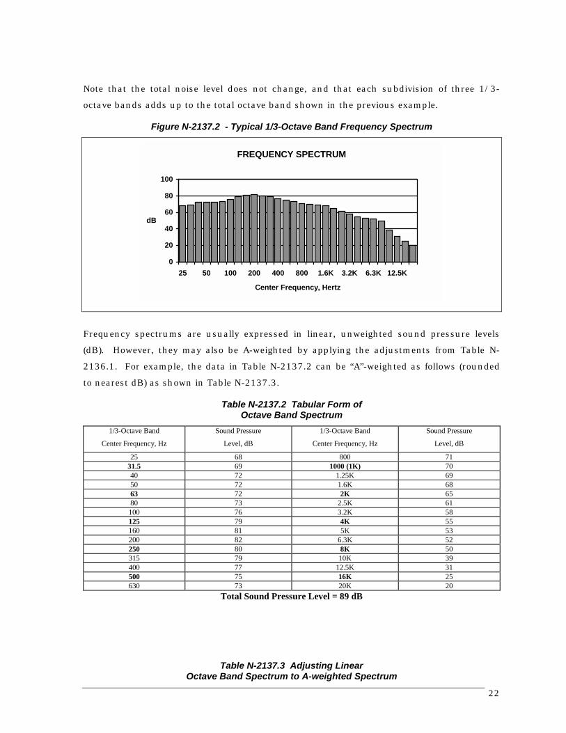
Note that the total noise level does not change, and that each subdivision of three 1/3-
octave bands adds up to the total octave band shown in the previous example.
Figure N-2137.2 - Typical 1/3-Octave Band Frequency Spectrum
FREQUENCY SPECTRUM
0
20
40
60
80
100
25 50 100 200 400 800 1.6K 3.2K 6.3K 12.5K
Center Frequency, Hertz
dB
Frequency spectrums are usually expressed in linear, unweighted sound pressure levels
(dB). However, they may also be A-weighted by applying the adjustments from Table N-
2136.1. For example, the data in Table N-2137.2 can be “A”-weighted as follows (rounded
to nearest dB) as shown in Table N-2137.3.
Table N-2137.2 Tabular Form ofOctave Band Spectrum
1/3-Octave Band
Center Frequency, Hz
Sound Pressure
Level, dB
1/3-Octave Band
Center Frequency, Hz
Sound Pressure
Level, dB
25 68 800 7131.5 69 1000 (1K) 7040 72 1.25K 6950 72 1.6K 6863 72 2K 6580 73 2.5K 61100 76 3.2K 58125 79 4K 55160 81 5K 53200 82 6.3K 52250 80 8K 50315 79 10K 39400 77 12.5K 31500 75 16K 25630 73 20K 20
Total Sound Pressure Level = 89 dB
Table N-2137.3 Adjusting LinearOctave Band Spectrum to A-weighted Spectrum

23
Octave Band
Center Frequency, Hz
Sound Pressure
Level, dBA
31.5 75 - 39 = 36
63 77 - 26 = 51
125 84 - 16 = 68
250 85 - 9 = 76
500 80 - 3 = 77
1000 (1K) 75 - 0 = 75
2000 (2K) 70 + 1 = 71
4000 (4K) 61 + 1 = 62
8000 (8K) 54 - 1 = 53
16000 (16K) 32 -7 = 25
Total Sound Pressure Level = 89 dB(Lin), and 81.5 dBA
The total A-weighted noise level now becomes 81.5 dBA, compared with the linear noise
level of 89 dB. In other words, the original linear frequency spectrum with a total noise
level of 89 dB sounded to the human ear as having a total noise level of 81.5 dBA.
However, a linear noise level of 89 dB with a different frequency spectrum, could have
produced a different A-weighted noise level, either higher or lower. The reverse may also be
true. Actually, there are theoretically an infinite amount of frequency spectrums that could
produce either the same total linear noise level or the same A-weighted spectrum. This is
an important concept, because it can help explain a variety of phenomena dealing with
noise perception. For instance, some evidence suggests that changes in frequencies are
sometimes perceived as changes in noise levels, even though the total A-weighted noise
levels do not change significantly. Sec. N-8000 (Special Problems) deals with some of these
phenomena.
N-2138 White Noise, Pink Noise
White noise is noise with a special frequency spectrum that has the same amplitude (level)
for each frequency interval over the entire audible frequency spectrum. It is often
generated in laboratories for calibrating sound level measuring equipment, specifically its
frequency response. One might expect that the octave or third-octave band spectrum of
white noise would be a straight line. This is, however, not true. Beginning with the lowest
audible octave, each subsequent octave spans twice as many frequencies than the previous
ones, and therefore contains twice the energy. This corresponds with a 3 dB step increase
for each octave band, and 1 dB for each third octave band.

24
Pink noise, in contrast, is defined as having the same amplitude for each octave band (or
third-octave band), rather than for each frequency interval. Its octave or third-octave band
spectrum is truly a straight, “level” line over the entire audible spectrum. Pink noise
generators are therefore conveniently used to calibrate octave or third-octave band
analyzers.
Both white and pink noise sound somewhat like the static heard from a radio that is not
tuned to a particular station.
N-2140 Sound PropagationFrom the source to the receiver noise changes both in level and frequency spectrum. The
most obvious is the decrease in noise as the distance from the source increases. The
manner in which noise reduces with distance depends on the following important factors:
• Geometric Spreading from Point and Line Sources
• Ground Absorption
• Atmospheric Effects and Refraction
• Shielding by Natural and Manmade Features, Noise Barriers, Diffraction, and
Reflection
N-2141 Geometric Spreading from Point and Line Sources
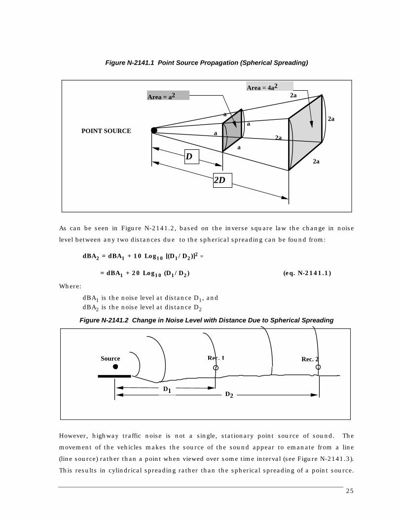
Sound from a small localized source (approximating a "point" source) radiates uniformly
outward as it travels away from the source in a spherical pattern. The sound level
attenuates or drops-off at a rate of 6 dBA for each doubling of the distance (6 dBA/DD).
This decrease, due to the geometric spreading of the energy over an ever increasing area, is
referred to as the inverse square law. Doubling the distance increases each unit area,
represented by squares with sides “a” in Figure N-2141.1, from a2 to 4a2.
Since the same amount of energy passes through both squares, the energy per unit area at
2D is reduced 4 times from that at distance D. Thus, for a point source the energy per unit
area is inversely proportional to the square of the distance. Taking 10 log10 (1/4) results in
a 6 dBA reduction (for each doubling of distance). This is the point source attenuation rate
for geometric spreading.
25
Figure N-2141.1 Point Source Propagation (Spherical Spreading)
As can be seen in Figure N-2141.2, based on the inverse square law the change in noise
level between any two distances due to the spherical spreading can be found from:
dBA2 = dBA1 + 10 Log10 [(D1/D2)]2 =
= dBA1 + 20 Log10 (D1/D2) (eq. N-2141.1)
Where:
dBA1 is the noise level at distance D1, anddBA2 is the noise level at distance D2
Figure N-2141.2 Change in Noise Level with Distance Due to Spherical Spreading
However, highway traffic noise is not a single, stationary point source of sound. The
movement of the vehicles makes the source of the sound appear to emanate from a line
(line source) rather than a point when viewed over some time interval (see Figure N-2141.3).
This results in cylindrical spreading rather than the spherical spreading of a point source.
a
aa
a
2a
2a
2a
2a
Area = a2Area = 4a2
D
2D
POINT SOURCE
Source Rec. 2
D1 D2
Rec. 1

26
Since the change in surface area of a cylinder only increases by two times for each doubling
of the radius instead of the four times associated with spheres, the change in sound level is
3 dBA per doubling of distance. The change in noise levels for a line source at any two
different distances due to the cylindrical spreading becomes:
dBA2 = dBA1 + 10 Log10 (D1/D2) (eq. N-2141.2)
Where:
dBA1 is the noise level at distance D1, and conventionally the known noise level
dBA2 is the noise level at distance D2 , and conventionally the unknown noise
level
Note: the expression 10 Log10 (D1/D2) is negative when D2 is greater than D1, positive
when D1 is greater than D2, and the equation therefore automatically accounts for the
receiver being farther out or closer in with respect to the source (Log10 of a number less
than 1 gives a negative result; Log10 of a number greater than 1 is positive, and Log10 (1) =
0).
Figure N-2141.3 Line Source Propagation (Cylindrical Spreading)
N-2142 Ground Absorption
Most often, the noise path between the highway and the observer is very close to the
ground. Noise attenuation from ground absorption and reflective wave canceling adds to
the attenuation due to geometric spreading. Traditionally, the access attenuation has also
been expressed in terms of attenuation per doubling of distance. This approximation is
done for simplification only, and for distances of less than 60 m (200 feet) prediction results
based on this scheme are sufficiently accurate. The sum of the geometric spreading
attenuation and the excess ground attenuation (if any) is referred to as the attenuation rate,
aa
b 2b
Area = ab
Area = 2ab
D
2D
Line Source

27
or drop-off rate. For distances of 60 m (200 feet) or greater the approximation causes
excessive inaccuracies in predictions. The amount of excess ground attenuation depends
on the height of the noise path and the characteristics of the intervening ground or site. In
practice this excess ground attenuation may vary from nothing to 8-10 dBA or more per
doubling of distance. In fact, it varies as the noise path height changes from the source to
the receiver and also changes with vehicle type since the source heights are different. The
complexity of terrain is another factor that influences the propagation of sound by
potentially increasing the number of ground reflections. Only the most sophisticated
computer model(s) can properly account for the interaction of soundwaves near the ground.
In the mean time, for the sake of simplicity two site types are currently used in traffic noise
models:
1. HARD SITES - These are sites with a reflective surface between the source and the
receiver such as parking lots or smooth bodies of water. No excess ground
attenuation is assumed for these sites and the changes in noise levels with distance
(drop-off rate) is simply the geometric spreading of the line source or 3 dBA/DD
(6dBA/DD for a point source).
2. SOFT SITES - These sites have an absorptive ground surface such as soft dirt,
grass or scattered bushes and trees. An excess ground attenuation value of 1.5
dBA/DD is normally assumed. When added to the geometric spreading results in
an overall drop-off rate of 4.5 dBA/DD for a line source (7.5 dBA/DD for a point
source).
The combined distance attenuation of noise due to geometric spreading and ground
absorption in the above simplistic scheme can be generalized with the following formulae:
dBA2 = dBA1 + 10 Log10 (D1/D2)1 + αααα ((((Line Source) (eq. N-2142.1)
dBA2 = dBA1 + 10 Log10 (D1/D2)2 + αααα (Point Source) (eq. N-2141.2)
where: αααα is a site parameter which takes on the value of 0 for a hard site and 0.5
for a soft site.
The above formulae may be used to calculate the noise level at one distance if the noise
level at another distance is known. The “αααα scheme” is just an approximation. It is used in
older versions of the FHWA Highway Traffic Noise Prediction Model. Caltrans research has
shown that for average traffic and “soft site” characteristics, the αααα scheme is fairly accurate
within 30 m (100 ft) from a typical highway. Between 30 - 60 m (100 - 200 ft) form a
28
highway, the algorithm results in average over predictions (model predicted noise levels
higher than actual) of 2 dBA. At 60 - 150 m (200 - 500 ft) over predictions average about 4
dBA.
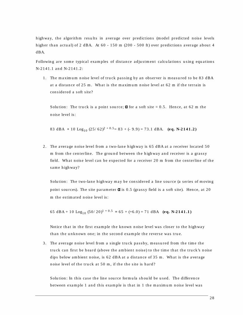
Following are some typical examples of distance adjustment calculations using equations
N-2141.1 and N-2141.2:
1. The maximum noise level of truck passing by an observer is measured to be 83 dBA
at a distance of 25 m. What is the maximum noise level at 62 m if the terrain is
considered a soft site?
Solution: The truck is a point source; αααα for a soft site = 0.5. Hence, at 62 m the
noise level is:
83 dBA + 10 Log10 (25/62)2 + 0.5= 83 + (- 9.9) = 73.1 dBA. (eq. N-2141.2)
2. The average noise level from a two-lane highway is 65 dBA at a receiver located 50
m from the centerline. The ground between the highway and receiver is a grassy
field. What noise level can be expected for a receiver 20 m from the centerline of the
same highway?
Solution: The two-lane highway may be considered a line source (a series of moving
point sources). The site parameter αααα is 0.5 (grassy field is a soft site). Hence, at 20
m the estimated noise level is:
65 dBA + 10 Log10 (50/20)1 + 0.5 = 65 + (+6.0) = 71 dBA (eq. N-2141.1)
Notice that in the first example the known noise level was closer to the highway
than the unknown one; in the second example the reverse was true.
3. The average noise level from a single truck passby, measured from the time the
truck can first be heard (above the ambient noise) to the time that the truck’s noise
dips below ambient noise, is 62 dBA at a distance of 35 m. What is the average
noise level of the truck at 50 m, if the the site is hard?
Solution: In this case the line source formula should be used. The difference
between example 1 and this example is that in 1 the maximum noise level was

29
measured. The maximum noise level is an instantaneous noise level, occurring at
one location only: presumably the closest point to the observer. In this example the
noise was an average noise level, i.e. the truck noise was measured at many
different locations representing the entire passby and therefore a series of point
sources that may be represented by a line source. Hence, eq. N-2141.1 should be
used with α α α α = 0. The answer is 60.5 dBA at 50 m.
Table N-2142.1 shows a simple generalization regarding the use of point or line source
distance attenuation equations for various source types, instantaneous noise and time-
averaged noise levels.
Sec. N-5500 contains additional discussions on how to use the appropriate drop-off rate in
the noise prediction models.
Table N-2142.1 Use of Point and Line Source Distance Attenuation Equations.
NOISE LEVEL AT STATIONARY RECEIVERS
SOURCE TYPE INSTANTANEOUS(Usually maximum)
TIME-AVERAGED
Single, Stationary PointSource (e.g. idling truck,pump, machinery)
Use Point Source Equation(eq. N-2142.2)
Use Point SourceEquation
(eq. N-2142.2)Single, Moving PointSource (e.g. movingtruck):
Use Point Source Equation(eq. - N 2142.2)
Use Line Source Equation(eq. N-2142.1)
Series of Point Souces ona Line, Stationary orMoving: (e.g. highwaytraffic)
Use Line Source Equation(eq. N-2142.1)
Use Line Source Equation(eq. N-2142.1)
N-2143 Atmospheric Effects and Refraction
Research by Caltrans and others has shown that atmospheric conditions can have a
profound effect on noise levels within 60 m (200 ft) from a highway. Wind has shown to be
the single most important meteorological factor within approximately 150 m (500 ft), while
vertical air temperature gradients are more important over longer distances. Other factors
such as air temperature and humidity, and turbulence, also have significant effects.
Wind. The effects of wind on noise are mostly confined to noise paths close to the ground.
The reason for this is the wind shear phenomenon. Wind shear is caused by the slowing
down of wind in the vicinity of a ground plane due to friction. As the surface roughness of

30
the ground increases, so does the friction between the ground and the air moving over it.
As the wind slows down with decreasing heights it creates a sound velocity gradient (due to
differential movement of the medium) with respect to the ground. This velocity gradient
tends to bend sound waves downward in the same direction of the wind and upward in the
opposite direction. The process, called refraction, creates a noise "shadow" (reduction)
upwind from the source and a noise "concentration" (increase) downwind from the
source. Figure N-2143.1 shows the effects of wind on noise. Wind effects on noise levels
along a highway are very much dependent on wind angle, receiver distance and site
characteristics. A 10 km/hr (6 mph) cross wind can increase noise levels at 75 m (250 ft)
by about 3 dBA downwind, and reduce noise by about the same amount upwind. Present
policies and standards ignore the effects of wind on noise levels. Unless winds are
specifically mentioned, noise levels are always assumed to be for zero winds. Noise
analyses are also always made for zero wind conditions.
Wind also has another effect on noise measurements. Wind "rumble" caused by friction
between air and a microphone of a sound level meter can contaminate noise measurements
even if a windscreen is placed over the microphone.
Limited measurements performed by Caltrans in 1987 showed that wind speeds of about 5
m/s produce noise levels of about 45 dBA, using a 1/2 inch microphone with a wind
screen. This means that noise measurements of less than 55 dBA are contaminated by
wind speeds of 5 m/s. A noise level of 55 dBA is about at the low end of the range of noise
levels routinely measured near highways for noise analyses. FHWA document No. FHWA-
DP-45-1R, titled “Sound Procedures for Measuring Highway Noise: Final Report”, August
1981, recommends that highway noise measurements should not be made at wind speeds
above 12 mph (5.4 m/s). A 5 m/s criterion for maximum allowable wind speed for routine
highway noise measurements seems reasonable and is therefore recommended. More
information concerning wind/microphone contamination will be covered in the noise
measurement section N-3000 of this Appendix.

31
Figure N-2143.1 - Wind Effects on Noise Levels
Wind turbulence. - Turbulence also has a scattering effect on noise levels, which is
difficult to predict at this time. It appears, however, that turbulence has the greatest effect
on noise levels in the vicinity of the source.
Temperature gradients - Figure N-2143.2 shows the effects of temperature gradients on
noise levels. Normally, air temperature decreases with height above the ground. This is
called the normal lapse rate, which for dry air is about - 1o C/100 m. Since the speed of
sound decreases as air temperature decreases, the resulting temperature gradient creates a
sound velocity gradient with height. Slower speeds of sound higher above the ground tend
to refract sound waves upward in the same manner as wind shear does upwind from the
source. The result is a decrease in noise. Under certain stable atmospheric conditions,
however, temperature profiles are inverted, or temperatures increase with height either
from the ground up, or at some altitude above the ground. This inversion results in
speeds of sound that temporarily increase with altitude, causing noise refraction similar to
that caused by wind shear downwind from a noise source. Or, once trapped within an
elevated inversion layer, noise may be carried over long distances in a channelized fashion.
Both ground and elevated temperature inversions have the effect of propagating noise with
less than the usual attenuation rates, and therefore increase noise. The effects of vertical
temperature gradients are more important over longer distances.
Wind Velocity
UpwindNoiseDecrease
DownwindNoiseIncrease

32
Figure N-2143.2 - Effects of Temperature Gradients on Noise
a. No Temperature Gradient - Reference(Speed of sound stays same with altitude)
b. Normal Lapse Rate - Noise Decrease(Speed of sound decreases with altitude)
c. Temperature Inversion - Noise Increase(Speed of sound increases with altitude)
Speed of Sound Speed of Sound
Speed of Sound
Speed of Sound Speed of Sound
Speed of Sound
Source
Ground
Source
Ground
Source
Ground

33
Temperature and humidity - Molecular absorption in air also reduces noise levels with
distance. Although this process only accounts for about 1 dBA per 300 m (1000 ft) under
average conditions of traffic noise in California, the process can cause significant longer
range effects. Air temperature, and humidity affect molecular absorption differently
depending on the frequency spectrum, and can vary significantly over long distances, in a
complex manner.
Rain. - Wet pavement results in an increase in tire noise and a corresponding increase in
frequencies of noise at the source. Since the propagation of noise is frequency dependent,
rain may also affect distance attenuation rates. On the other hand, traffic generally slows
down during rain, decreasing noise levels and lowering frequencies. When wet, different
pavement types interact differently with tires than when they are dry. These factors make
it very difficult to predict noise levels during rain. Hence, no noise measurements or
predictions are made for rainy conditions. Noise abatement criteria and standards do not
address rain.
N-2144 Shielding by Natural and Man-made Features, Noise Barriers,Diffraction, and ReflectionA large object in the path between a noise source and a receiver can significantly attenuate
noise levels at that receiver. The amount of attenuation provided by this “shielding”
depends on the size of the object, and frequencies of the noise levels. Natural terrain
features, such as hills and dense woods, as well as manmade features, such as buildings
and walls can significantly alter noise levels. Walls are often specifically used to reduce
noise.
Trees and Vegetation - For a vegetative strip to have a noticeable effect on noise levels it
must be dense and wide. A stand of trees with a height that extends at least 5 m (16 ft)
abve the line of sight between source and receiver, must be at least 30 m (100 ft) wide and
dense enough to completely obstruct a visual path to the source to attenuate traffic noise
by 5 dBA. The effects appear to be cumulative, i.e. a 60 m (200 ft) wide stand of trees
would reduce noise by an additional 5 dBA. However, the limit is generally a total
reduction of 10 dBA. The reason for the 10 dBA limit for any type of vegetation is that
sound waves passing over the tree tops (“sky waves”) are frequently refracted back to the
surface, due to downward atmospheric refraction caused by wind, temperature gradients,
and turbulence.
Landscaping - Caltrans research has shown that ordinary landscaping along a highway
accounts for less than 1 dBA reduction. Claims of increases in noise due to removal of
vegetation along highways are mostly spurred by the sudden visibility of the traffic source.
34
There is evidence of the psychological "out of sight, out of mind" effect of vegetation on
noise.
Buildings - Depending on the site geometry, the first row of houses or buildings next to a
highway may shield the second and successive rows. This is often the case where the
facility is at-grade or depressed. The amount of noise reduction varies with house or
buildig sizes, spacing of houses or buildings, and site geometry. Generally, for an at-grade
facility in an average residential area where the first row houses cover at least 40% of total
area (i.e. no more than 60% spacing) , the reduction provided by the first row is reasonably
assumed at 3 dBA, and 1.5 dBA for each additional row. For example, behind the first row
we may expect a 3 dBA noise reduction, behind the second row 4.5 dBA, third row 6 dBA,
etc. For houses or buildings “packed” tightly, (covering about 65-90% of the area, with 10-
35% open space), the first row provides about 5 dBA reduction. Successive rows still
reduce 1.5 dBA per row. Once again, and for the reason mentioned in the above vegetation
discussion, the limit is 10 dBA. For these assumptions to be true, the first row of houses
or buidings must be equal to or higher than the second row, which should be equal to or
higher than the third row, etc.
Noise Barriers - Although technically any natural or man-made feature between source
and receiver that reduces noise is a noise barrier, the term is generally reserved for either a
wall or a berm that is specifically constructed for that purpose. The acoustical design of
noise barriers is covered in sections N-4000 (Traffic Noise Model) and N-6000 (Acoustical
Barrier Design Considerations). However, it is appropriate at this time to introduce the
acoustical concepts associated with noise barriers. These principles loosely apply to any
obstacle between source and receiver.
Referring to Figure N-2144.1, when a noise barrier is inserted between a noise source and
receiver, the direct noise path along the line of sight between the two is interrupted. Some
of the acoustical energy will be transmitted through the barrier material and continue to the
source, albeit at a reduced level. The amount of this reduction depends on the material’s
mass and rigidity, and is called the Transmission Loss.
The Transmission Loss (TL) is expressed in dB and its mathematical expression is:
TL = 10log10(Ef/Eb) (eq. N-2144.1)
where: Ef = the relative noise energy immediately in front (source side) of the barrier
Eb = The relative noise energy immediately behind the barrier (receiver side)

35
Figure N-2144.1 - Alteration of Sound Paths After Inserting a Noise Barrier Between Sourceand Receiver.
Note that Ef and Eb are relative energies, i.e. energies with reference to the energy of 0 dB
(see section N-2134). As relative energies they may be expressed as any ratio (fractional or
percentage) that represents their relationship. For instance if 1 percent of the noise energy
striking the barrier is transmitted, TL = 10log10(100/1)= 20 dBA. Most noise barriers have
TL’s of 30 dBA or more. This means that only 0.1 percent of the noise energy is
transmitted.
The remaining direct noise (usually close to 100 percent) is either partially or entirely
absorbed by the noise barrier material (if sound absorptive), and/or partially or entirely
reflected (if the barrier material is sound reflective). Whether the barrier is reflective or
absorptive depends on its ability to absorb sound energy. A smooth hard barrier surface
such as masonry or concrete is considered to be almost perfectly reflective, i.e.almost all
the sound striking the barrier is reflected back toward the source and beyond. A barrier
surface material that is porous with many voids is said to be absorptive, i.e. little or no
sound is reflected back. The amount of energy absorbed by a barrier surface material is
expressed as an absorption coefficient α, which has a value ranging from 0 (100%
reflective) to 1 (100% absorptive). A perfect reflective barrier (α=0) will reflect back virtually
all the noise energy (assuming a transmission loss of 30 dBA or greater) towards the
opposite side of a highway. If we ignore the difference in path length between the direct
and reflected noise paths to the opposite (unprotected) side of a highway, the maximum
expected increase in noise will be 3 dBA.
If we wish to calculate the noise increase due to a partially absorptive wall we may use eq.
N-2144.1. Ef in this case is still the noise energy striking the barrier, but Eb now becomes
DIRECT TRANSMITTED
DIFFRACTED
REFLECTED
SOURCE
NOISEBARRIER
RECEIVER
ABSORBED
A
SHADOWZONE

36
the energy reflected back. For example, a barrier material with an α of 0.6 absorbs 60% of
the direct noise energy and reflects back 40%. To calculate the increase in noise on the
opposite side of the highway in this situation the energy loss from the transformation of the
total noise striking the barrier to the reflected noise energy component is 10log10(100/40)=
4 dBA. In other words, the energy loss of the reflection is 4 dBA. If the direct noise level of
the source at a receiver on the opposite side of the highway is 65 dBA, the reflective
component (ignoring the difference in distances traveled) will be 61 dBA. The total noise
level at the receiver is the sum of 65 and 61 dBA, or slightly less than 66.5 dBA. The
reflected noise caused an increase of 1.5 dBA at the receiver.
Referring back to Figure N-2144.1, we have discussed the direct, transmitted, absorbed,
and reflected noise paths. These represent all the variations of the direct noise path due to
the insertion of the barrier. Of those, only the transmitted noise reaches the receiver behind
the barrier. There is, however, one more path, which turns out to be the most imported
one, that reaches the receiver. The noise path that before the barrier insertion was directed
towards “A” is diffracted downward towards the receiver after the barrier insertion.
In general, diffraction is characteristic of all wave phenomena (including light, water, and
sound waves). It can best be described as the “bending” of waves around objects . The
amount of diffraction depends on the wavelength and the size of the object. Low frequency
waves with long wavelengths approaching the size of the object, are easily diffracted.
Higher frequencies with short wavelengths in relation to the size of the object, are not as
easily diffracted. This explains why light, with its very short wavelengths casts shadows
with fairly sharp, well defined edges between light and dark. Sound waves also “cast a
shadow” when they strike an object. However, because of their much longer wavelengths
(by at least a half dozen or so orders of magnitude) the “noise shadows” are not very well
defined and amount to a noise reduction, rather than an absence of noise.
Because noise consists of many different frequencies that diffract by different amounts, it
seems reasonable to expect that the greater the angle of diffraction is, the more frequencies
will be attenuated. In Figure N-2144.1, beginning with the top of the shadow zone and
going down to the ground surface, the higher frequencies will be attenuated first, then the
middle frequencies and finally the lower ones. Notice that the top of the shadow zone is
defined by the extension of a straight line from the noise source (in this case represented at
the noise centroid as a point source) to the top fo the barrier. The diffraction angle is
defined by the top of the shadow zone and the line from the top of the barrier to the
receiver. Thus, the position of the source relative to the top of the barrier determines the
extent of the shadow zone and the diffraction angle to the receiver. Similarly, the receiver

37
location relative to the top of the barrier is also important in determinig the diffraction
angle.
From the previous discussion, three conclusions are clear. First, the diffraction
phenomenon depends on three critical locations, that of the source, the top of barrier, and
the reciver. Second, for a given source, top of barrier and receiver configuration, a barrier
is more effective in attenuating higher frequencies than lower frequencies (see Figure N-
2144.2). Third, the greater the angle of diffraction, the greater the noise attenuation is.
Figure N-2144.2 - Diffraction of Sound Waves
The angle of diffraction is also related to the path length difference (δ) between the direct
noise and the diffracted noise. Figure N-2144.3 illustrates the concept of path length
difference. A closer examination of this illustration reveals that as the diffraction angle
becomes greater, so does δ. The path length difference is defined as δ = a+b-c. If the
horizontal distances from source to receiver and source to barrier, and also the differences
in elevation between source, top barrier and receiver are known, a,b, and c can readily be
calculated. Assuming that the source in Figure N-2144.3 is a point source, a, b, and c are
calculated as follows:
a = [d ( ) ]12
2 12+ −h h
b = ( )d h22
22+
c = ( )d h212+
Source
Barrier
High Frequencies
Low Frequencies
38
Figure N-2144.3 - Path Length Difference Between Direct and Diffracted Noise Paths.
Highway noise prediction models use δ in the barrier attenuation calculations. Section N-
5500 covers the subject in greater detail. However, it is appropriate to include the most
basic relationship between δ and barrier attenuation by way of the so-called Fresnel
Number (N0). If the source is a line source (such as highway traffic) and the barrier is
infinitely long, there are an infinite amount of path length differences. The path length
difference (δ0)at the perpendicular line to the barrier is then of interest.
Mathematically, N0 is defined as:
N0 = 2(δδδδ0/λλλλ) (eq. N-2144.2)
where: N0 = Fresnel Number determined along the perpendicular linebetween source and receiver (i.e. barrier must be perpendicular to the direct noise path)
δ0 = δ measured along the perpendicular line to the barrier
λ = wavelength of the sound radiated by the source.
According to eq. N-2131.1, λ = c/f , and we may rewrite eq. N-2144.2:
N0 = 2(fδδδδ0/c) (eq. N-2144.3)
where: f = the frequency of the sound radiated by the sourcec = the speed of sound
c
ab
h1
h2d1
d
d2
SOURCE
RECEIVER
TOPBARRIER
PATH LENGTH DIFFERENCE (δ)δ)δ)δ) = a+b-c
Diffraction Angle

39
Note that the above equations relate δ0 to N0. If one increases, so does the other, and
barrier attenuation increases as well. Similarly, if the frequency increases, so will N0, and
barrier attenuation. Figure N-2144.4 shows the barrier attenuation ∆B for an infinitely long
barrier, as a function of 550 Hz (typical “average” for traffic).
Figure N-2144.4 - Barrier Attenuation (∆∆∆∆B) vs Fresnel Number (N0), for Infinitely Long Barriers
There are several “rules of thumb” for noise barriers and their capability of attenuating
traffic noise. Figure N-2144.5 illustrates a special case where the top of the barrier is just
high enough to “graze” the direct noise path, or line of sight between source and receiver.
In such an instance the noise barrier provides 5 dBA attenuation.
Figure N-2144.5 - Direct Noise Path “Grazing” Top Barrier Results in 5 dBA Attenuation
Another situation, where the direct noise path is not interrupted but still close to the
barrier, will provide some noise attenuation. Such “negative diffraction” (with an associated
-25
-20
-15
-10
−5
.01 .1 1 10 100
N0
∆∆∆∆ΒΒΒΒ,,,,
dB
SOURCE
NOISEBARRIER
RECEIVERDIRECT, “GRAZING”
ATTENUATION: 5 dBA

40
“negative path length difference and “negative Fresnel Number”) generally occurs when the
direct noise path is within 1.5 m (5 ft) above the top of barrier for the average traffic source
and receiver distances encountered in near highway noise environments. The noise
attenuation provided by this situation is between 0 - 5 dBA: 5 dBA when the noise path
approaches the grazing point and near 0 dBA when it clears the top of barrier by
approximately 1.5 m (5 ft) or more.
Figure N-2144.6 - “Negative Diffraction” Provides Some Noise Attenuation
The aforementioned principles of barriers loosely apply to terrain features (such as berms,
low ridges, as well as other significant manmade features). The principles will be discussed
in greater detail in sections N-5500 and N-6000.
N-2200 EFFECTS OF NOISE; NOISE DESCRIPTORS
N-2210 Human Reaction to Sound
People react to sound in a variety of ways. For example, rock music may be pleasant to
some people while for others it may be annoying, constitute a health hazard and/or disrupt
activities. Human tolerance to noise depends on a variety of acoustical characteristics of
the source, as well as environmental characteristcs. These factors are briefly discussed
below:
1. Level, variability in level (dynamic range), duration, frequency spectrums and time
patterns of noise. Exposures to very high noise levels can damage hearing. A high
level is more objectionable than a low level noise, and intermittent truck peak noise
levels are more objectionable than the continuous level of fan noise. Humans have
better hearing sensitivities in the high frequency region than in the low. This is
reflected in the A-scale (section N-2136) which de-emphasizes the low frequency
SOURCE
NOISEBARRIER
RECEIVERNEGATIVE DIFFRACTION
ATTENUATION: < 5 dBA
41
sounds. Studies indicate that the annoyance or disturbance correlates with the A-
scale.
2. The amount of background noise present before the intruding noise. People tend to
compare an intruding noise with the existing background noise. If the new noise is
readily identifiable or considerably louder than the background or ambient, it
usually becomes objectionable. An aircraft flying over a residential area is an
example.
3. The nature of the work or living activity that is exposed to the noise source. Highway
traffic noise might not be disturbing to workers in a factory or office, but the same
noise might be annoying or objectionable to people sleeping at home or studying in
a library. An automobile horn at 2:00 a.m. is more disturbing than the same noise
in traffic at 5:00 p.m.
N-2211 Human Response to Changes in Noise Levels
Under controlled conditions in an acoustics laboratory, the trained healthy human ear is
able to discern changes in sound levels of 1 dBA, when exposed to steady, single frequency
(“pure tone”) signals in the mid-frequency range. Outside of such controlled conditions, the
trained ear can detect changes of 2 dBA in normal environmental noise. It is widely
accepted that the average healthy ear, however, can barely perceive noise level changes of 3
dBA.
Earlier, we discussed the concept of "A" - weighting and the reasons for describing noise in
terms of dBA. The human response curve of frequencies in the audible range is simply not
linear, i.e. humans do not hear all frequencies equally well.
It appears that the human perception of loudness is also not linear, neither in terms of
decibels, nor in terms of acoustical energy. We have already seen that there is a
mathematical relationship between decibels and relative energy. For instance, if one source
produces a noise level of 70 dBA, two of the same sources produce 73 dBA, three will
produce about 75 dBA, and ten will produce 80 dBA.
Human perception is complicated by the fact that it has no simple correlation with
acoustical energy. Two noise sources do not "sound twice as loud" as one noise source.
Based on the opinions of thousands of subjects tested by experts in the field, however,
some approximate relationships between changes in acoustical energy and corresponding
human reaction have been charted. The results have been summarized in Table N-2211.1,
which shows the relationship between changes in acoustical energy, dBA and human
perception. The table shows the relationship between changes in dBA (∆dBA), relative

42
energy with respect to a reference of a ∆dBA of 0 (no change), and average human
perception. The factor change in relative energy relates to the change in acoustic energy.
Figure N-2211.1Relationship Between Noise Level Change, Factor Change in Relative Energy,and Perceived Change
Perceived Change
Noise Level
Change,
∆∆∆∆dBA
Change in
Relative
Energy,
10±±±±∆∆∆∆dBA/10
Perceived Change in
Percentage,
(2±±±±∆∆∆∆dBA/10-1) x 100%
Descriptive Change in Perception
+ 40 dBA 10,000 x Sixteen Times as Loud
+ 30 dBA 1,000 x Eight Times as Loud
+20 dBA 100 x + 300 % Four Times as Loud
+ 15 dBA 31.6 x + 183 %
+ 10 dBA 10 x + 100 % Twice as Loud
+ 9 dBA 7.9 x + 87 %
+ 8 dBA 6.3 x + 74 %
+ 7 dBA 5.0 x + 62 %
+ 6 dBA 4.0 x + 52 %
+5 dBA 3.16 x + 41 % Readily Perceptible Increase
+4 dBA 2.5 x + 32 %
+ 3 dBA 2.0 x + 23 % Barely Perceptible Increase
0 dBA 1 0 % REFERENCE (No change)
- 3 dBA 0.5 x - 19 % Barely Perceptible Reduction
- 4 dBA 0.4 x - 24 %
- 5 dBA 0.316 x - 29 % Readily Perceptible Reduction
- 6 dBA .25 x - 34 %
- 7 dBA 0.20 x - 38 %
- 8 dBA 0.16 x - 43 %
- 9 dBA 0.13 x -46 %
- 10 dBA 0.10 x - 50 % Half as Loud
- 15dBA 0.0316 x - 65 %
- 20 dBA 0.01 x - 75 % One Quarter as Loud
- 30 dBA 0.001 x One Eighth as Loud
- 40 dBA 0.0001 x One Sixteenth as Loud
Section N-2133 mentioned that the r.m.s. value of the sound pressure ratio squared (P1/ P2
is proportional to the energy content of sound waves (acoustic energy).
Human perception is displayed in two columns (percentage and descriptive). The

43
percentage of perceived change is based on the mathematical approximation that the factor
change of human perception relates to ∆dBA by the following:
Factor Change in Perceived Noise Levels = 2±±±±∆∆∆∆dBA/10 (eq. N-2211.1)
According to the above approximation, the average human ear perceives a 10 dBA decrease
in noise levels as half of the original level (2±∆dBA/10 = 2 -10/10 = 0.5). By subtracting 1 andmultiplying by 100 the result will be in terms of a percentage change in perception, where apositive (+) change represents an increase, and a negative (-) change a decrease. Thedescriptive perception column puts into words how the percentage change is perceived.
N-2220 Describing NoiseNoise in our daily environment fluctuates over time. Some of the fluctuations are minor,
some are substantial; some occur in regular patterns, others are random. Some noise
levels fluctuate rapidly, others slowly. Some noise levels vary widely, others are relatively
constant. In order to describe noise levels, we need to choose the proper noise descriptor or
statistic.
N-2221 Time PatternsFigure N-2221.1 is a graphic representation of how noise can have different time patterns
depending on the source. Shown are noise level vs. time patterns of four different sources:
a fan (a), a pile driver (b), a single vehicle passby (c), and highway traffic (d).
Figure N-2221.1 - Different Noise Level Vs. Time Patterns
The simplest noise level time pattern is that of constant noise (a), which is essentially a
straight and level line. Such a pattern is characteristic of stationary fans, compressors,
pumps, air conditioners, etc. At each instant the noise level is about the same for a fixed
observer. A single measurement taken at random, would suffice to describe the noise level
a. Constant (e.g. fan) b. Impacts (e.g. pile driver)
c. Single Vehicle Pass by d. Traffic
T I M E
dBA

44
at a specific distance. The minimum and maximum noise level would be nearly the same
as the average noise level.
Other noise level vs. time patterns are more complicated. For instance, to describe the pile
driving noise (b), noise samples need to include the instantaneous “peaks” or maximum
noise levels. In our environment, there are a whole range of noises of many different
patterns in addition to the ones shown in Figure 2220.1. The levels may be extremely short
in duration such as a single gun shot (transient noise), or intermittent such as the pile
driver, or continuous as was the case with the fan. Traffic noise along major highways
tends to lie somewhere between intermittent and continuous (d). It is characterized by the
somewhat random distribution of vehicles, each of which emits a pattern such as shown in
(c).
N-2222 Noise Descriptors
To choose the proper noise descriptor, we have to know the nature of the noise source and
also how we want to describe it. Are we interested only in the maximum levels, the average
noise levels, the percentage of time above a certain level, or the levels that are exceeded
10%, 50% or 90% of the time? How can we compare the noise of a fast flying jet aircraft -
loud but short in duration - with a slower but quieter propeller airplane? It is easy to see that
the proper descriptor depends on the spatial distribution of noise source(s), duration,
amount of fluctuation, and time patterns.
There are dozens of descriptors and scales which have been devised over the years to
quantify community noise, aircraft fly-overs, traffic noise, industrial noise, speech
interference, etc. The descriptors shown in Table N-2222.1 are the ones most often
encountered in traffic, community, and environmental noise. There are many more
descriptors, but they are not mentioned here. The word "LEVEL", abbreviated L, is
frequently used whenever sound is expressed in decibels relative to the reference pressure.
Thus, all of the descriptors shown in Table N-2222.1 have "L" as part of the term.
All Caltrans highway traffic noise analysis should be done in terms of worst noise hour
Leq(h). If a noise analysis requires other descriptors (to satisfy city or county requirements)
then see section N-2230 for a discussion of descriptor conversions.
Table N- 2222.1. Common Noise Descriptors.

45
NOISE DESCRIPTOR DEFINITION
LMAX (Maximum Noise Level) The highest instantaneous noise level during a
specified time period. This descriptor is sometimes
referred to as “peak (noise) level”. The use of “peak”
level should be discouraged because it may be
interpreted as a non-r.m.s. noise signal (see sec. N-
2133 for difference between peak and r.m.s.)
LX (A Statistical Descriptor) The noise level exceeded X percent of a specified time period.
The value of X is commonly 10. Other values of 50 and 90 are
sometimes also used. Examples: L10, L50, L90.
Leq (Equivalent Noise Level. Routinely used by Caltrans and
FHWA to address the worst noise hour (Leq(h)).
The equivalent steady state noise level in a stated period of time
that would contain the same acoustic energy as the time varying
noise level during the same period.
Ldn (Day - Night Noise Level. Used commonly for describing
community noise levels).
A 24-hour Leq with a "penalty"of 10 dBA added during the night
hours (2200 - 0700). The penalty is added because this time is
normally sleeping time.
CNEL (Community Noise Equivalent Level. A common
community noise descriptor; also used for airport noise).
Same as the Ldn with an additional penalty of 4.77 dBA, (or 10
Log 3), for the hours 1900 to 2200, usually reserved for relaxation,
TV, reading, and conversation.
SEL (Single Event Level. Used mainly for aircraft noise; it
enables comparing noise created by a loud, but fast overflight,
with that of a quieter, but slow overflight).
The acoustical energy during a single noise event, such as an
aircraft overflight, compressed into a period of one second,
expressed in decibels.
N-2223 Calculating Noise Descriptors
The following formulae and examples may be used to calculate various noise descriptors
from instantaneous noise vs time data.
Lx - The Lx, a statistical descriptor, signifies the noise level that is exceeded x% of the time.
This descriptor was formerly used in highway noise (before the Leq). The most common
value of x was 10, denoting the level that was exceeded 10% of the time. Hence, the L10
descriptor will be used as an example to represent the Lx family of calculations. The
following instantaneous noise samples (Table 2223.1) shown as a frequency distribution
(dBA vs number of occurrences), will serve to illustrate the L10 calculation.
The total No. of samples taken at 10 second intervals was 50. For the L10 we therefore
need to find the 5 highest values (10% of 50). These are exceeding the L10. In the above

46
data set, we can simply count down from the top. The “boundary” of the top 10 % lies at 76
dBA. Therefore the L10 lies at 76 dBA. The L50 would be 66 dBA (25 occurrences from the
top), etc.
Table N-2223.1 Noise Samples for L10 CalculationNoise Level, dBA Occurrences (Sampling Interval 10 seconds)
(Each X is one occurrence)
Total No. of
Occurrences
80 0
79 0
78 X 1
77 X 1
76 X X X 3
75 X X 2
74 X X 2
73 X X 2
72 0
71 X X X 3
70 X 1
69 X X 2
68 X X X X X 5
67 X X 2
66 X X X X 4
65 X X X X X X X 7
64 X X X X X 5
63 X X X 3
62 X X X 3
61 X X 2
60 X X 2
Total No. of Samples 50
Leq - The Leq descriptor is a special sort of average noise level. Instead of averaging decibel
levels, the energy levels are averaged. The Leq is also called an energy-mean noise level.
The instant noise levels over a certain time period are energy-averaged by first converting
all dBA values to relative energy values. Next, these values are added up and the total is
divided by the number of values. The result is average (relative) energy. The final step then
is to convert the average energy value back to a decibel level. Section N-2135, equation N-
2135.3 showed the method of adding the energy values. This equation can be expanded to
yield an Leq:
Leq = 10log10[(10SPL(1)/10+10SPL(2)/10 + ... 10SPL(n)/10)/N] (eq. N-2223.1)
Where: SPL(1), SPL(2), SPL(n) = the 1st, 2nd, and nth noise level
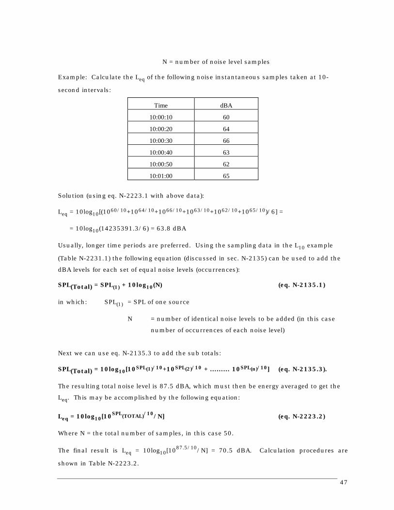
47
N = number of noise level samples
Example: Calculate the Leq of the following noise instantaneous samples taken at 10-
second intervals:
Time dBA
10:00:10 60
10:00:20 64
10:00:30 66
10:00:40 63
10:00:50 62
10:01:00 65
Solution (using eq. N-2223.1 with above data):
Leq = 10log10[(1060/10+1064/10+1066/10+1063/10+1062/10+1065/10)/6] =
= 10log10(14235391.3/6) = 63.8 dBA
Usually, longer time periods are preferred. Using the sampling data in the L10 example
(Table N-2231.1) the following equation (discussed in sec. N-2135) can be used to add the
dBA levels for each set of equal noise levels (occurrences):
SPL(Total) = SPL(1) + 10log10(N) (eq. N-2135.1)
in which: SPL(1) = SPL of one source
N = number of identical noise levels to be added (in this case
number of occurrences of each noise level)
Next we can use eq. N-2135.3 to add the sub totals:
SPL(Total) = 10log10[10SPL(1)/10+10SPL(2)/10 + ......... 10SPL(n)/10] (eq. N-2135.3).
The resulting total noise level is 87.5 dBA, which must then be energy averaged to get the
Leq. This may be accomplished by the following equation:
Leq = 10log10[10SPL(TOTAL)/10/N] (eq. N-2223.2)
Where N = the total number of samples, in this case 50.
The final result is Leq = 10log10[1087.5/10/N] = 70.5 dBA. Calculation procedures are
shown in Table N-2223.2.

48
Table N-2223.2 - Noise Samples for Leq CalculationNoise Level,
dBA
Occurrences (Sampling Interval 10 seconds)
(Each X is one occurrence)
No. of
Occurrences
(N)
Total Noise Levels
dBA + 10log10(N)
80 0
79 0
78 X 1 78
77 X 1 77
76 X X X 3 80.8
75 X X 2 78
74 X X 2 77
73 X X 2 76
72 0
71 X X X 3 75.8
70 X 1 70
69 X X 2 72
68 X X X X X 5 75
67 X X 2 70
66 X X X X 4 72
65 X X X X X X X 7 73.5
64 X X X X X 5 71
63 X X X 3 67.8
62 X X X 3 66.8
61 X X 2 64
60 X X 2 63
Totals 50 87.5
Leq = 10 Log10 [(108.75)/50] = 70.5 dBA
Ldn - The Ldn descriptor is actually a 24 hour Leq, or the energy-averaged result of 24 1-
hour Leq‘s, with the exception that the night-time hours (defined as 2200 - 0600 hours) are
assessed a 10 dBA “penalty”. This attempts to account for the fact that nighttime noise
levels are potentially more disturbing than equal daytime noise levels.
Mathematically this “day-night” descriptor is expressed as:
Ldn = 10 Log10[( 1
24) 10
1
24
i =�
Leq(h)i + Wi/10] (eq.N-2223.3)
where: Wi = 0 for day hours (0700 - 2200)
Wi = 10 for night hours (2200 - 0700)
Leq(h)i = Leq(for the ith hour)

49
To calculate an Ldn accurately, we must have 24 successive hourly Leq‘s, representing one
typical day. The hourly values between 2200-0700 (9 hourly values) must first be weighted
by adding 10 dBA. An example is shown in Table N-2223.3.
The energy average calculated from the 9 weighted and 15 unweighted hourly Leq‘s is the
Ldn. Once the hourly data is properly weighted, the Ldn can be calculated as an Leq (in this
case a weighted 24 hour Leq). We may use eq. N-2223.1 with the weighted data. The
resulting Ldn is 65 dBA.
Table N-2223.3 Noise Samples for Ldn CalculationsBeginHour
Leq(h),
dBA
Weight,dBA
WeightedNoise,dBA
BeginHour
Leq(h),
dBA
Weight,dBA
WeightedNoise,dBA
00:00 54 +10 64 12:00 65 0 65
01:00 52 +10 62 13:00 65 0 65
02:00 52 +10 62 14:00 63 0 63
03:00 50 +10 60 15:00 65 0 65
04:00 53 +10 63 16:00 65 0 65
05:00 57 +10 67 17:00 63 0 63
06:00 62 +10 72 18:00 64 0 64
07:00 65 0 65 19:00 62 0 62
08:00 63 0 63 20:00 60 0 60
09:00 64 0 64 21:00 58 0 58
10:00 66 0 66 22:00 57 +10 67
11:00 66 0 66 23:00 55 +10 65
CNEL - The CNEL is the same as the Ldn EXCEPT for an additional weighting of almost 5
dBA for the evening hours of 1900 - 2200. The equation is essentially the same as eq. N-
2223.3, with an additional definition of Wi= 10Log10(3), which is 4.77. Calculations for
CNEL are done similarly to those for Ldn. The result is normally about 0.5 dBA higher
than that of an Ldn using the same 24-hour data. Following is the equation for the CNEL.:
CNEL = 10 Log10[( 1
24) 10
1
24
i =�
Leq(h)i + Wi/10] (eq.N-2223.4)
Where: Wi = 0 for day hours (0700 - 1900)
Wi = 10log10(3) = 4.77 for evening hours (1900 - 2200)

50
Wi = 10 for night hours (2200 - 0700)
Leq(h)i = Leq(for the ith hour)
The above 24-hour data used in the Ldn example, yields a CNEL of 65.4 dBA, as compared
to 65.0 dBA for the Ldn.
SEL - The SEL is useful in comparing the acoustical energy of different events involving
different source characteristics. For instance, the over flight of a slow propeller driven
plane may not be as loud as a jet aircraft, but the former is slower and therefore lasts
longer than the jet noise. The SEL makes a noise comparison of both events possible,
because it combines the effects of time and level. For instance, the Leq of a steady noise
level will remain unchanged over time. It will be the same when calculated for a time
period of 1 second or 1000 seconds. The SEL of a steady noise level, however, will keep
increasing, because all the acoustical energy within a given time period is included in the
reference time period of one second. Since both values are energy-weighted they are
directly related to each other by time as shown in the following equations:
SEL = Leq(T)+10log10(T) (eq. N-2223.5)
Leq(T) = SEL+10log10(1/T) = SEL-10log10(T) (eq. N-2223.6)
where: T = the duration of the noise level in seconds.
Example: The Leq of a 65-second aircraft over flight is 70 dBA. What is the SEL?
Solution (using eq. N-2223.2): SEL = Leq(65 sec)+10log10(65) = 70+18.1 = 88.1 dBA.
N-2230 Conversion Between Noise Descriptors
Although Caltrans exclusively uses the Leq descriptor, there are some times that
comparisons need to be made with local noise standards, most of which are in terms of Ldn
or CNEL. Twenty-four hour noise data are often not available. Following is a methodology
that allows a reasonably accurate conversion of the worst hourly noise level to a Ldn or
CNEL.
N-2231 Leq To Ldn/CNEL, and Vice Versa.
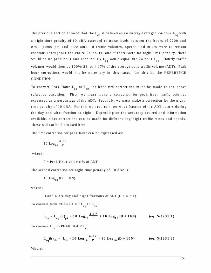
51
The previous section showed that the Ldn is defined as an energy-averaged 24-hour Leq with
a night-time penalty of 10 dBA assessed to noise levels between the hours of 2200 and
0700 (10:00 pm and 7:00 am). If traffic volumes, speeds and mixes were to remain
constant throughout the entire 24 hours, and if there were no night time penalty, there
would be no peak hour and each hourly Leq would equal the 24-hour Leq. Hourly traffic
volumes would then be 100%/24, or 4.17% of the average daily traffic volume (ADT). Peak
hour corrections would not be necessary in this case. Let this be the REFERENCE
CONDITION.
To convert Peak Hour Leq to Ldn, at least two corrections must be made to the above
reference condition. First, we must make a correction for peak hour traffic volumes
expressed as a percentage of the ADT. Secondly, we must make a correction for the night-
time penalty of 10 dBA. For this we need to know what fraction of the ADT occurs during
the day and what fraction at night. Depending on the accuracy desired and information
available, other corrections can be made for different day/night traffic mixes and speeds.
These will not be discussed here.
The first correction for peak hour can be expressed as:
10 Log10 4.17
P
where :
P = Peak Hour volume % of ADT
The second correction for night time penalty of 10 dBA is:
10 Log10 (D + 10N)
where :
D and N are day and night fractions of ADT (D + N = 1)
To convert from PEAK HOUR Leq to Ldn :
Ldn = Leq (h)pk + 10 Log10 4.17
P + 10 Log10 (D + 10N) (eq. N-2231.1)
To convert Ldn to PEAK HOUR Leq:
Leq(h)pk = Ldn - 10 Log10 4.17
P - 10 Log10 (D + 10N) (eq. N-2231.2)
Where:

52
Leq(h)pk = Peak Hour Leq
P = Peak Hour volume % of ADT
D = Day-time fraction of ADT
N = Night-time fraction of ADT
Note: (D + N) must equal 1
Example: The peak hour Leqat a receiver near a freeway is 65.0 dBA; the peak hour traffic
is 10% of the ADT; the day-time traffic volume is .85 of the ADT; the night-time
traffic volume is .15 of the ADT. Assume that the day and night-time heavy
truck percentages are equal and traffic speeds do not vary significantly. What is
the estimated Ldn at the receiver?
Solution:
Ldn = 65.0 + 10 Log10 4.1710 + 10 Log10 (0.85 + 1.50)
= 65.0 + (-3.8) + 3.70
= 64.9 dBA
Note that in the above example, which is a fairly typical case, the Ldn is approximately
equal to the Leq(h)pk. The rule of thumb is that Ldnis within +/- 2 dBA of the Leq(h)pk under
normal traffic conditions.
The values in the following Table N-2231.1 can also be used in equations N-2231.2 and N-
2231.3. Notice that the “peak hour %” term of the equation always yields a negative value,
while the weighted “day/night split” always yields a positive value. The difference between
the two is the difference between the Leq(h)pk and the Ldn.
Table N-2231.1 - Leq/Ldn Conversion Factors

53
P, % 10Log10(4.17/P) D N 10 Log10(D+10N)
5 -0.8 0.98 0.02 +0.76 -1.6 0.95 0.05 +1.67 -2.3 0.93 0.07 +2.18 -2.8 0.90 0.10 +2.89 -3.3 0.88 0.12 +3.210 -3.8 0.85 0.15 +3.711 -4.2 0.83 0.17 +4.012 -4.6 0.80 0.20 +4.513 -4.9 0.78 0.22 +4.714 -5.3 0.75 0.25 +5.115 -5.6 0.73 0.27 +5.417 -6.1 0.70 0.30 +5.720 -6.8 0.68 0.32 +5.9
0.65 0.35 +6.20.63 0.37 +6.40.60 0.40 +6.6
Figure N-2231.1 shows the difference between Leq(h)pk and Ldn graphically. For example if
P is 10% and D/N = 0.85/0.15, the Ldn ≈ Leq(h)pk.
Figure N-2231.1 - Relationship Between Ldn and Leq(h)pk
If CNEL is desired, the Ldn to CNEL corrections (∆) in Table N-2231.2 may be used.
1.00 0.95 0.90 0.85 0.80 0.75 0.70 0.65 0.60 D0.00 0.05 0.10 0.15 0.20 0.25 0.30 0.35 0.40 N
40
35
30
25
20
15
10
5
0
0 dBA
-1 dBA
-2 dBA
-3 dBA
+1 dBA+2 dBA+3 dBA
P %
D/N SPLIT
Ldn = Leq(h)pk +

54
Table N-2231.2 - Ldn/CNEL Corrections (∆∆∆∆); must be added to Ldn to obtain CNEL.
d E(CNEL = Ldn + ∆∆∆∆)
∆∆∆∆
0.80 0.05 0.3
0.79 0.06 0.4
0.78 0.07 0.5
0.77 0.08 0.5
0.76 0.09 0.6
0.75 0.10 0.7
0.74 0.11 0.7
0.73 0.12 0.8
0.72 0.13 0.8
0.71 0.14 0.9
0.70 0.15 0.9
The values shown assume a fixed night time fractional traffic contribution of 0.15 (D/N
split of .85/.15 for Ldn). The remaining day time traffic contribution of .85 is further
subdivided into day (d) and evening (E) hours. In each instance, d+E = 0.85.
N-2240 Negative Effects on HumansThe most obvious negative effects of noise are physical damage to hearing. Other obvious
effects are the interference of noise with certain activities, such as sleeping, conversation,
etc. Less obvious, but nevertheless very real, are the stress effects of noise. A brief
discussion of each of the topics follows.
N-2241 Hearing Damage.
A person exposed to high noise levels can suffer hearing damage. The damage may be
gradual or traumatic. These are described as follows:
1. Gradual. Sustained exposure to moderately high noise levels over a period of timecan cause gradual hearing loss. It starts out as a temporary hearing loss, such asimmediately after a loud rock concert. The hearing usually restores itself within afew hours after exposure, although not quite to its pre-exposure level. This is alsocalled a temporary threshold shift. Although the permanent deterioration may benegligible, it will become significant after many repetitions of the exposure. At thattime, it is labeled permanent hearing damage. The main causes of permanentdamage are daily exposure to industrial noise. Transportation noise levelsexperienced by communities and the general public are normally not high enough toproduce hearing damage.
2. Traumatic. Short and sudden exposure to an extremely high noise level, such as agun shot or explosion at very close range can cause a traumatic hearing loss. Sucha loss is very sudden and can be permanent.
Hearing damage is preventable by reducing the exposure to loud noise. This can be done
by quieting the source, shield the receiver by a barrier, or having the receiver wear proper

55
ear protection. Occupational exposure to noise is controlled by the Occupational Safety
and Health Agency (OSHA), and is based on a maximum allowable noise exposure level of
90 dBA for 8 hours. For each halving of the exposure time, the maximum noise level is
allowed to increase 5 dBA. Thus, the maximum allowable noise exposure (100 %) is 90
dBA for 8 hours, 95 dBA for 4 hours, 100 dBA for 2 hours, 105 dBA for 1 hour, 110 dBA
for 30 minutes, and 115 dBA for 15 minutes. Dosimeters, worn by workers in noisy
environments, can measure noise during the workday in percentages of the maximum daily
exposure.
N-2242 Interference with Activities.
Activities most affected by noise include rest, relaxation, recreation, study and
communications. Although most interruptions by noise can be considered annoying, some
may be considered dangerous. An example would be the inability to hear warning signals
or verbal warnings in noisy industrial situations, or in situations involving workers next to
a noisy freeway. Figure N-2242.1 gives an estimate of the speech communication that is
possible at various noise levels and distances.
Figure N-2242.1 - Interference of Conversation due to Background NoisedBA
BACKGROUND
NOISE
120
110
100
90
80
70
60
50
40
0 1.5 3 4.5 6 7.5 9 10.5TALKER TO LISTENER DISTANCE, m
CONVERSATIONIMPOSSIBLE
CONVERSATIONDIFFICULT
CONVERSATIONPOSSIBLE
NEAR - NORMALCONVERSATION (Normal Voice)
(Shout)
(Maximum Vocal Effort)
56
For instance, if the talker to listener distance is 6 m, normal conversation can be conducted
with the background level at about 50 dBA. If the background level is increased to 60 dBA,
the talker must either raise his/her voice, or decrease the distance to the listener to 3 m.
N-2243 Stress Related Diseases
There is ample evidence that noise can cause stress in humans, and thus may be
responsible for a host of stress-related diseases, such as hypertension, anxiety, heart
disease, etc. Although noise is probably not the sole culprit in these diseases, it can be a
contributor. The degree of how much noise contributes to stress related diseases, depends
on noise frequencies, their band widths, noise levels, and time patterns. In general, higher
frequency, pure tone, and fluctuating noise tend to be more stressful than lower frequency,
broad band, and constant-level noise.

TECHNICAL NOISE SUPPLEMENTOctober 1998
N-57
N-3000 MEASUREMENTS & INSTRUMENTATIONNoise measurements play an important role in noise analysis and acoustical design of noise
attenuation for transportation projects. This section covers recommendations on why,
where, when, and how noise measurements should be taken. A brief discussion on
available instrumentation is also included. Because of the variety of sound
instrumentation, coverage of equipment setup and operational procedures has been kept at
a general level. For greater detail, manufacturers' manuals should be consulted.
The noise analyst should be aware of the importance as well as the limitations of noise
measurements. As is the case with all field work, quality noise measurements are relatively
expensive. They take time, personnel and equipment. The noise analyst should therefore
carefully plan the locations, times, duration, and number of repetitions of noise
measurements before actually taking the measurements. A conscientious effort should be
made during the measurements to document site, traffic and meteorology and other
pertinent factors discussed in this section.
The contents of this section are consistent with methods described in the Federal Highway
Administration (FHWA) document FHWA-DP-45-1R, “Sound Procedures for Measuring
Highway Noise: Final Report”, August 1981, and FHWA-PD-96-046, “Measurement of
Highway -Related Noise”, May 1996.
N-3100 PURPOSES OF NOISE MEASUREMENTSThere are five major purposes for measuring transportation noise. These purposes are to:
1. Determine existing ambient and background noise levels
2. Calibrate noise prediction models
3. Monitor construction noise levels for compliance with Standard Specifications,
Special Provisions, and Local Ordinances
4. Evaluate the effectiveness of abatement measures such as noise barriers
5. Perform special studies and research
Ambient and background noise and model calibration measurements are routinely
performed by the Districts. Construction noise monitoring is also frequently done by the
Districts. Some Districts conduct before-and-after noise abatement measurements.
Special studies and noise research measurements, however, are done rarely by the Districts
and are often contracted out to consultants with Caltrans oversight.

TECHNICAL NOISE SUPPLEMENTOctober 1998
N-58
Where, when, and how noise measurements are performed depends on the purpose of the
measurements. The following sections discuss the reasons for the above measurements,
what they include, and how the results are used.
N-3110 Ambient and Background Noise Levels
Ambient noise levels are all-encompassing noise levels at a given place and time, usually a
composite of sounds from all sources near and far, including specific sources of interest.
Typically, ambient noise levels include highway plus community noise levels. Ambient noise
levels are measured for the following reasons:
• To assess highway traffic noise impacts for new highway construction or
reconstruction projects. Existing ambient noise levels provide a baseline for
comparison to predicted future noise levels. The measurements are also used to
describe the current noise environment in the area of the proposed project. This
information is reported in appropriate environmental documents. Generally, the
noise resulting from the natural and mechanical sources and human activity,
considered to be usually present, should be included in the measurements.
• To prioritize retrofit noise barrier sites along existing freeways. The measured noise
levels are part of a formula used to calculate a priority index. Prioritization is
required by Section 215.5 of the Streets and Highways Code. The measured noise
levels are also used to design retrofit noise barriers.
• To investigate citizens' traffic or construction noise complaints. Noise
measurements are usually reported in a memo to the interested party or parties,
with recommendations for further actions or reasons why further actions are not
justified.
Background noise is the total of all noise in a specific region without the presence of noise
sources of interest. Typically, this would be the noise generated within the community,
without the highway, and is usually measured at locations away from the highway where
highway noise does not contribute to the total noise level. Background noise levels are
typically measured to determine the feasibility of noise abatement and to insure that noise
reduction goals can be achieved. Noise abatement cannot reduce noise levels below
background. Section N-6160 discusses the importance of background noise levels.
Depending on the situation, the noise sources to be measured may typically include
highway traffic, community noise, surface street traffic, train noise, and sometimes airplane
noise (when project is near an airport).

TECHNICAL NOISE SUPPLEMENTOctober 1998
N-59
N-3120 Model Calibration
Noise measurements near highways or other transportation corridors are routinely used to
calibrate the computer models by comparing calculated noise levels with actual (measured)
noise levels. The calculated levels are modeled results obtained from traffic counts and
other parameters recorded during the noise measurements. The difference between
calculated and measured noise levels may then be applied to calculated future noise levels
assuming site conditions will not change significantly, or modeled existing noise levels (see
sections N-5400 and N-5330). Obviously, model calibration can only be performed on
projects involving existing highways.
N-3130 Construction Noise Levels
These measurements are frequently done by Districts to check for the contractor's
compliance with the standard specifications and special provisions of a transportation
construction project, and with local ordinances.
N-3140 Performance of Abatement Measures
Before-and-after abatement measurements can be used to evaluate the performance of
noise barriers, building insulation, or other abatement options. The measurements provide
a "systems check" on the design and construction procedures of the abatement. Although
these measurements are done occasionally by some Districts, they are not part of a routine
program.
N-3150 Special Studies and Research
These measurements are usually done by the NT,M&R. They may involve District
assistance and generally involve noise research projects. Setups are usually complex and
include a substantial amount of equipment and personnel positioned at many locations for
simultaneous noise measurement. The studies generally require more sophisticated
equipment than that used for routine noise studies.
N-3200 MEASUREMENT LOCATIONSThe selection of measurement locations requires a considerable amount of planning and
foresight by the noise analyst. A fine balance must be achieved between a sufficient
amount of quality locations on one side, and the cost in person hours on the other. Good
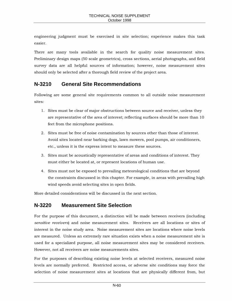
TECHNICAL NOISE SUPPLEMENTOctober 1998
N-60
engineering judgment must be exercised in site selection; experience makes this task
easier.
There are many tools available in the search for quality noise measurement sites.
Preliminary design maps (50 scale geometrics), cross sections, aerial photographs, and field
survey data are all helpful sources of information; however, noise measurement sites
should only be selected after a thorough field review of the project area.
N-3210 General Site Recommendations
Following are some general site requirements common to all outside noise measurement
sites:
1. Sites must be clear of major obstructions between source and receiver, unless they
are representative of the area of interest; reflecting surfaces should be more than 10
feet from the microphone positions.
2. Sites must be free of noise contamination by sources other than those of interest.
Avoid sites located near barking dogs, lawn mowers, pool pumps, air conditioners,
etc., unless it is the express intent to measure these sources.
3. Sites must be acoustically representative of areas and conditions of interest. They
must either be located at, or represent locations of human use.
4. Sites must not be exposed to prevailing meteorological conditions that are beyond
the constraints discussed in this chapter. For example, in areas with prevailing high
wind speeds avoid selecting sites in open fields.
More detailed considerations will be discussed in the next section.
N-3220 Measurement Site Selection
For the purpose of this document, a distinction will be made between receivers (including
sensitive receivers) and noise measurement sites. Receivers are all locations or sites of
interest in the noise study area. Noise measurement sites are locations where noise levels
are measured. Unless an extremely rare situation exists when a noise measurement site is
used for a specialized purpose, all noise measurement sites may be considered receivers.
However, not all receivers are noise measurements sites.
For the purposes of describing existing noise levels at selected receivers, measured noise
levels are normally preferred. Restricted access, or adverse site conditions may force the
selection of noise measurement sites at locations that are physically different from, but

TECHNICAL NOISE SUPPLEMENTOctober 1998
N-61
acoustically equivalent to the intended receivers. In some cases measurements are not
feasible at all. In such cases the existing noise levels must be modeled. This can only be
accomplished along an existing facility.
Generally, there are more modeled receivers than noise measurement sites. It is far less
expensive to take noise measurements at selected, representative receivers and model
results for the rest. Nevertheless, there needs to be an adequate overlap of measurement
sites and modeled receivers for model calibration and verification.
The following factors should be considered when selecting noise measurement sites.
N-3221 Site Selection By Purpose of Measurement
Noise measurement sites should be selected according to the purpose of the measurement.
For example, if the objective is to determine noise impacts of a highway project, sites
should be selected in regions that will be exposed to the highest noise levels generated by
the highway after completion of the project. The sites should also represent areas of human
use.
Conversely, if the objective is to measure background community noise levels, the sites
should be located in areas that represent the community, without influence from the
highway. These measurements are often necessary for acoustical noise barrier design (see
section 6150) and to document before project noise levels at distant recievers. Past
controversies concerning unsubstantiated increases in noise levels at distant receivers,
attributed to noise barriers could have readily been resolved if sufficient background noise
receivers would have been selected (see Section N-8200) after the project has been built.
Classroom noise measurements (Street and Highways Code Section 216), or receivers
lacking outside human use, require inside - as well as outside - noise measurements in
rooms with worst noise exposures from the highway. Measurements should generally be
made at a point in a room, hall or auditorium where people would be impacted by
infiltrating noise from the sources of interest. These are typically desks, chairs, or beds
near windows. Several sensitive points may have to be tested and results averaged. No
measurements should be made within 3-4 feet of a wall. It is also important to take
measurements in the room in its typical furnished condition. If windows are normally
open, take measurements with windows open and closed. Fans, ventilation, clocks,
appliances, telephones, etc. should be turned off. People should preferably vacate the room
or be extremely quiet.

TECHNICAL NOISE SUPPLEMENTOctober 1998
N-62
Model calibration measurements usually require sites to be near the highway, preferably at
receivers or acoustical equivalents to the receivers. (See Model Calibration Section N-5400
for additional details).
Sites for construction noise monitoring are dictated by standard specifications, special
provisions, and local ordinances, which detail maximum allowable noise levels at a
reference distance: e.g. Lmax 86 dBA at 15 m (50 ft), or other requirements.
Before-and-after measurements for evaluations of noise barriers and other abatement
options, and measurements for special studies or research are non-routine and require a
detailed experimental design. Coordination with the NT,M&R is advisable.
N-3222 Site Selection By Acoustical Equivalence
Noise measurement sites should be representative of the areas of interest.
Representativeness in this case means acoustical equivalence. The concept of acoustical
equivalence incorporates equivalences in noise sources, distances from these sources,
topography, and other pertinent parameters.
The region under study may need to be subdivided into subregions in which acoustical
equivalence can generally be maintained. Boundaries of each subregion must be estimated
by one or more of the previously mentioned acoustical parameters. Also, in cases where
measurements are being taken for more than one purpose, separate sub-regions may be
defined by each purpose. The size of regions or subregions may vary from small to large.
For example, noise abatement for a school may cover one small region (the school), while a
noise study for a large freeway project may range from one large region to many subregions.
The number of measurement sites selected within each region or subregion under study
depends on its size, number of receivers, and remaining variations in acoustical
parameters. Obviously, the more conscientiously an effort is made to define acoustical
subregions, the less sites are needed within each subregion. The minimum number of sites
recommended for each region or subregion is two.
Figure N-3222.1 shows an example of receiver and noise measurement site selections for
an at-grade freeway widening and noise barrier project. Also shown are alternate noise
measurement sites to be used if the selected receivers are not accessible, or otherwise not
suitable for noise measurement locations. Only sites near the freeway are shown.
Background noise measurement sites would typically be off the map, further away from the
freeway. Actual site selection would depend on field reviews and more information not
shown on the map.
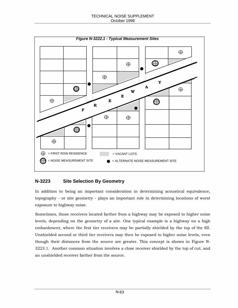
TECHNICAL NOISE SUPPLEMENTOctober 1998
N-63
N-3223 Site Selection By Geometry
In addition to being an important consideration in determining acoustical equivalence,
topography - or site geometry - plays an important role in determining locations of worst
exposure to highway noise.
Sometimes, those receivers located farther from a highway may be exposed to higher noise
levels, depending on the geometry of a site. One typical example is a highway on a high
embankment, where the first tier receivers may be partially shielded by the top of the fill.
Unshielded second or third tier receivers may then be exposed to higher noise levels, even
though their distances from the source are greater. This concept is shown in Figure N-
3223.1. Another common situation involves a close receiver shielded by the top of cut, and
an unshielded receiver farther from the source.
Y A W E E R F
= FIRST ROW RESIDENCE
= NOISE MEASUREMENT SITE = ALTERNATE NOISE MEASUREMENT SITE
= VACANT LOTS
Figure N-3222.1 - Typical Measurement Sites
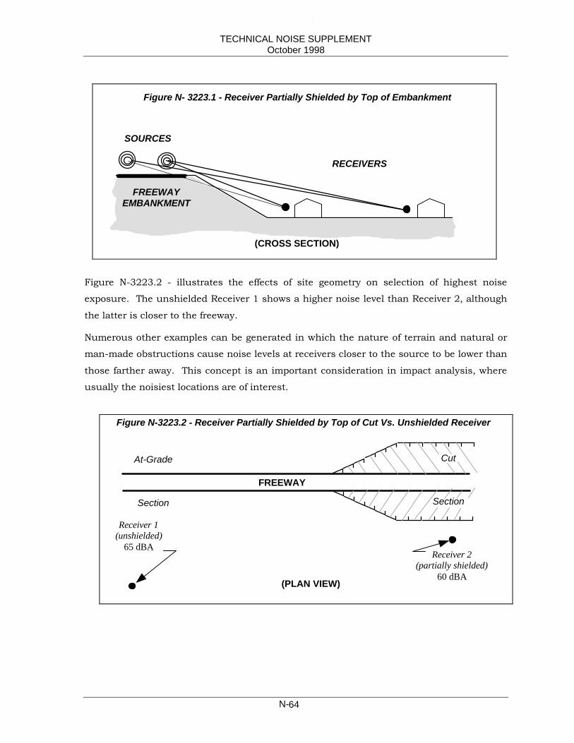
TECHNICAL NOISE SUPPLEMENTOctober 1998
N-64
Figure N-3223.2 - illustrates the effects of site geometry on selection of highest noise
exposure. The unshielded Receiver 1 shows a higher noise level than Receiver 2, although
the latter is closer to the freeway.
Numerous other examples can be generated in which the nature of terrain and natural or
man-made obstructions cause noise levels at receivers closer to the source to be lower than
those farther away. This concept is an important consideration in impact analysis, where
usually the noisiest locations are of interest.
(PLAN VIEW)
Receiver 1(unshielded)
65 dBAReceiver 2
(partially shielded)60 dBA
FREEWAY
At-Grade
Section
Cut
Section
Figure N-3223.2 - Receiver Partially Shielded by Top of Cut Vs. Unshielded Receiver
Figure N- 3223.1 - Receiver Partially Shielded by Top of Embankment
FREEWAYEMBANKMENT
SOURCES
RECEIVERS
(CROSS SECTION)
1
TECHNICAL NOISE SUPPLEMENTOctober 1998
N-65
N-3300 MEASURING TIMES, DURATION, AND NUMBEROF REPETITIONS
N-3310 Measuring Times
FHWA 23 CFR Part 772 requires that traffic characteristics which yield the worst hourly
traffic noise impact on a regular basis be used for predicting noise levels and assessing
noise impacts. Therefore, if the purpose of the noise measurements is to determine a future
noise impact by comparing predicted noise with measured, the measurements must reflect
the highest existing hourly noise level that occurs regularly. In some cases, weekly and/or
seasonal variations need to be taken into consideration. In recreational areas, weekend
traffic may be greater than on week days and, depending on the type of recreation, may be
heavily influenced by season.
Measurements made for retrofit noise barrier projects also require noise measurements
during the highest traffic noise hour.
The noise impact analysis for classrooms, under the provisions of the Streets and Highways
Code Section 216, requires noise measurements to be made "at appropriate times during
regular school hours ...." and sets an indoor noise limit of 52 dBA, Leq
(h), from freeway
sources. Therefore, noise measurements for schools qualifying for school noise abatement
under Section 216 need to be made during the noisiest-traffic hour during school hours.
Noise from school children often exceeds traffic noise levels. In order to avoid contaminated
measurements it is often necessary to evacuate class rooms for the duration of the
measurements, or take measurements during vacation breaks.
Noise measurements for model calibration do not have to be made during the highest noise
hour, but it is desirable to have about the same estimated traffic mix (heavy truck
percentages of the total volume) and traffic speeds as during the noisiest hour. Accurate
traffic counts and meteorological observations (see Section N-3600) must be made during
these measurements.
Noise monitoring for background community noise levels should preferably be done during
the expected time of the highest noise level from the highway, even though the
measurements are taken at sites that are far enough removed from an existing highway to
not be contaminated by it. The reason for this is that the background levels will later be
added to predicted near-highway noise levels.

TECHNICAL NOISE SUPPLEMENTOctober 1998
N-66
Noise monitoring for investigating citizen's complaints may have to be done at a mutually-
agreed-on time. Frequently, these measurements are taken before or after normal working
hours, as dictated by the nature of the complaint.
Construction monitoring is performed during operation of the equipment to be monitored.
This may require night work on some construction projects.
Unless other times are of specific interest, before and after noise abatement (e.g. noise
barrier) measurements to verify noise barrier performance should preferably be done during
the noisiest hour. There are several reasons for this. First, noise barriers are designed for
noisiest hour traffic characteristics, which probably include highest truck percentages, and
second, to minimize contamination by background noise. Traffic should be counted during
these measurements. If before and after traffic conditions are different, measurements
should be normalized or adjusted to the same conditions of traffic (see section N-3312).
The nature of special studies and research projects dictate the appropriate times for those
measurements.
N-3311 Noisiest Hour For Highway Traffic
The peak traffic hour is generally NOT the noisiest hour. During rush hour traffic, vehicle
speeds and heavy truck volumes are often low. Free flowing traffic conditions just before or
after the rush hours often yield higher noise levels. Preliminary noise measurements at
various times of the day are sometimes necessary to determine the noisiest hour.
If accurate traffic counts and speeds for various time periods are available, the noisiest
hour may be determined by using the prediction model.
Experience based on previous studies may also be of value in determining the noisiest hour
for a particular facility.
N-3312 Adjusting Other-Than-Noisiest Hour
For the sake of efficiency, highway traffic noise measurements are often not made when the
highest hourly traffic noise levels occur. These measurements may be adjusted upward to
noisiest hour levels by using the prediction model. To make the adjustments, traffic must
be counted and speeds determined simultaneously with the noise measurements. The
following procedure must be followed:
1. Take noise measurements and count traffic simultaneously during each
measurement. Although lane-by-lane traffic counts yield the most accurate results
it is usually sufficient to count traffic by direction (e.g. east bound and west bound).

TECHNICAL NOISE SUPPLEMENTOctober 1998
N-67
Separate vehicles in the three vehicle groups used by the model (autos, medium
trucks, and heavy trucks). Obtain average traffic speeds (both directions). These
may be obtained by radar or by driving a test vehicle through the project area at the
prevailing traffic speed.
2. Expand vehicle counts for the measurement period to hourly values: i.e., if the
measurement period was 15 minutes, multiply the vehicles counted in each group
by 4. (Section N-3320 discusses duration of measurement as a function of hourly
vehicle volumes).
3. Input the hourly traffic volumes and speeds (from steps 1 and 2) in the Highway
Traffic Noise Prediction Model. Also include the proper roadway/receiver geometry
and site parameters. Run model.
4. Input the traffic volumes and speeds associated with the noisiest hour and the same
roadway/receiver geometry and site parameters as used in step 3. Run model.
5. Subtract results of step 3 from those of step 4. (Step 4 results should always be
larger than step 3).
6. Add the differences obtained in step 5 to the noise measurements of step 1.
7. Example:
8. Measured noise level in step 1, Leq
= 66 dBA
9. Calculated for step 1 conditions (step 3) = 67 dBA
10. Calculated for noisiest hour (step 4) = 69 dBA
11. Difference (step 5) = 2 dBA
12. Measured noise level adjusted to noisiest hour (step 6)
= 66 dBA + 2 dBA = 68 dBA
If 24-hour monitoring equipment is available, a histogram of 24 hourly noise
measurements may be developed for an existing freeway. This information may then be
used to adjust an off-peak-hour noise level at any location along the freeway to a noisiest-
hour-noise level. However, steps must be taken to reduce the chance of undetected noise
contaminations, should they occur. Then, if hourly noise relationships are in agreement
between the two monitors, there is reasonable assurance that neither were contaminated.
There is, however, no assurance that regional contamination such as frequent aircraft fly-
overs did not take place., Hence, measurements with remote noise monitoring equipment

TECHNICAL NOISE SUPPLEMENTOctober 1998
N-68
must be approached with extreme caution and only with at least some familiarity of nearby
noise sources.
N-3320 Measurement Duration
A noise measurement representing an hourly Leq
does not need to last the entire hour. As
long as noise levels do not change significantly, a shorter time period will usually be
sufficient to represent the entire hour of interest. The recommended length of
measurements depends on how much the noise levels fluctuate. The greater the
fluctuations, the longer the measurement needs to be. Vehicle spacing and differences in
vehicle types are responsible for fluctuating noise levels. These fluctuations become less as
traffic densities increase. Highway noise also becomes more constant as the distance from
the highway increases because the rate of distance change between a moving vehicle and a
receiver diminishes.
The following durations are recommended for highway traffic noise measurements as a
function of number of vehicles per hour (vph) per lane (Table N-3320.1):
Table N-3320.1 - Suggested Measurement Durations
TrafficVolume
Veh./Hour/Lane Duration
High > 1000 10 MinutesMedium 500 - 1000 15-20 “Low < 500 20-30 “
Most sound level meters automatically integrate and digitally display cumulative Leq’s.
Near the beginning of each measurement period, the displays fluctuate considerably.
However, after more data is collected they tend to stabilize. The time it takes to stabilize
depends on the amount of noise fluctuations. A measurement may be terminated when the
range of the fluctuations in displayed Leq is less than 0.5 dBA. When in doubt, measure a
little longer.
N-3330 Number of Measurement Repetitions
Noise measurements taken at a specific site tend to vary from measurement to
measurement. The most common causes of these variations are:
1. Changes in traffic volumes, speeds, and/or mixes.
2. Contamination from other noise sources, such as barking dogs, aircraft, nearbyconstruction, etc.
3. Change in meteorology (wind speed, wind direction, temperature, humidity, etc.)
TECHNICAL NOISE SUPPLEMENTOctober 1998
N-69
4. Changes in site conditions
5. Instrument error
6. Operator error
7. Calibration error
8. Malfunctioning instruments
Because of these potential variables and errors that may occur during a measurement, it is
strongly recommended that a time averaged measurement (such as the Leq
descriptor) be
repeated AT LEAST once at each site. This procedure will reduce the chances of undetected
errors. There are exceptions to this recommendation. Whenever three or more noise
measurements are made in the same general area, either simultaneously or in relatively
rapid succession, one measurement at each site may be sufficient, if the sites are
acoustically equivalent (see Section N-3222). However, to determine if a measurement at
any particular site is acceptable, the measurement should be compared with those at the
other sites and subjected to the same criteria for repeat measurements discussed later in
this section.
The recommended minimum of two measurements should be taken independently (using
two different setups and separate calibrations). That, of course, does not preclude the
operator from taking more than one measurement per setup and calibration. As a matter of
fact, if time permits, multiple measurements during each setup are encouraged in order to
improve accuracy. The two setups may be made consecutively, at different times of day, or
on different days.
If done consecutively, the setup should be broken: power must be turned off and on and
instruments must be calibrated again. If a recording device - such as a graphic level
recorder (GLR) - is connected to a sound level meter (SLM), the device should also be turned
off and on and recalibrated. It is further recommended that equipment be disassembled
and reassembled to avoid undetected errors through bad connections in the cables or
microphone.
Repeat measurements should be compared with the original(s) under the same conditions
of traffic, meteorology and site. Noise contamination, instrument malfunction, operator
error, or any other anomalies in the measurements can then readily be detected. To insure
that conditions are the same for all measurements, traffic counts and some basic
meteorological measurements should be made during the noise measurements (see sections
N-3340 and N-3600).

TECHNICAL NOISE SUPPLEMENTOctober 1998
N-70
If the repeat measurements do not agree with the original(s), further repetitions will be
necessary. How close the measurements should agree depends on the purpose of the
measurements.
For routine measurements, such as determining ambient noise levels or calibrating noise
prediction models, the above recommended minimum of two measurements normalized for
differences in traffic mix and volumes should agree within 2 dBA. If more than one
measurement is taken per setup, the mean noise levels for the two setups should agree
within 2 dB. Repetitive measurements for each setup should then be within +/- 1 dBA of
the mean noise level of the setup.
The above criteria have been set empirically from many years of field experience with a
variety of sound level meters approved for transportation noise measurements (ANSI S1.4
1983, Types 1 and 2).
Following are some examples illustrating these criteria. They were purposely selected to
show the extreme allowable limits. Usually, better agreement between setups and within
setups can be expected. The examples assume that all meteorological conditions, traffic
conditions and site conditions are the same throughout all measurements.
Example 1 data:
Meas’ment No.Leq (dBA)
Setup 1 Setup 2(Example 1 measurements are acceptablebecause they agree by 2 dBA.)
1 74.5 76.5Mean 75.5 Use the mean of 2 measurements = 75.5 dBA
Example 2 data:
Meas’ment No.Leq (dBA)
Setup 1 Setup 2(Example 2 measurements are acceptablebecause the means of setups 1 and 2 agree
1 69 71 by 2 dBA, AND measurements within each2 67 69 setup are within ± 1 dBA of the setup’s mean.
Mean ofSetups
68 70
Mean of All 69 Use mean of all measurements = 69 dBA
Example 3 data:
Meas’ment No.Leq (dBA)
Setup 1 Setup 2(Example 3 measurements are acceptable)
1 61.6 58.62 59.6 -
Mean ofSetups
60.6 58.6
Mean of All 59.9 (round off to 60) Use mean of all measurements = 60 dBA

TECHNICAL NOISE SUPPLEMENTOctober 1998
N-71
The above examples indicate that as long as the agreement criteria between the two setups
and within each setup are met, all measurements can be averaged together.
Following are examples of what to do if the setups do not agree by 2 dBA:
Example 4 data:
Measurement Leq
(dBA) (Example 4 measurements are NOT
No. Setup 1 Setup 2 acceptable: )1 65.3 68.0
After the second measurement, a decision should be made to either take another
measurement during setup 2, or break the setup and take a measurement for a new setup
3. Either method will be acceptable. If the choice is to take another measurement during
setup 2, however, and the agreement criteria can still not be met, it is then recommended
to break setup 2 and perform additional measurement(s) with setup 3. If agreement is
reached between setups 2 and 3, then eliminate setup 1, as illustrated in example 5:
Example 5 data:
Measurement Leq
(dBA) (Setup 2 & 3 measurements areacceptable.)
No. Setup 1 Setup 2 Setup 31 65.3 68.0 69.02 - 68.5 - Mean of setup 2 and 3 = 68.5 dBA
If setup 3 measurement would have agreed with both setup 1 and 2 (say with 67.0, instead
of 69.0) then another decision would have to be made: a) use setups 1 and 3, b) use setups
2 and 3, or c) use the average of all three setups (all measurements). The safest approach
would then be to use the average of all measurements, unless there would be a good reason
to eliminate one setup.
The above examples illustrate some extreme cases. Obviously, many other combinations
are possible. Most measurements will show better agreement. The examples are intended
to show how the recommended criteria may be applied in general. Individual judgment and
experience may have to be relied on in more complicated situations.
In some cases greater accuracy is required than the criteria allow. These cases mostly
apply to special studies or research. However, they may also be applied to a few key noise
measurement sites on a large project for the purpose of accurate model calibration. In these
cases 95% confidence interval for the mean of several measurements (using a minimum of
two setups) can be calculated. The 95% confidence interval should be specified to be no
more than ± 1 dBA. Table N-3330.1 shows the maximum allowable standard deviations as
a function of number of samples (measurements). Although the table is calculated for up
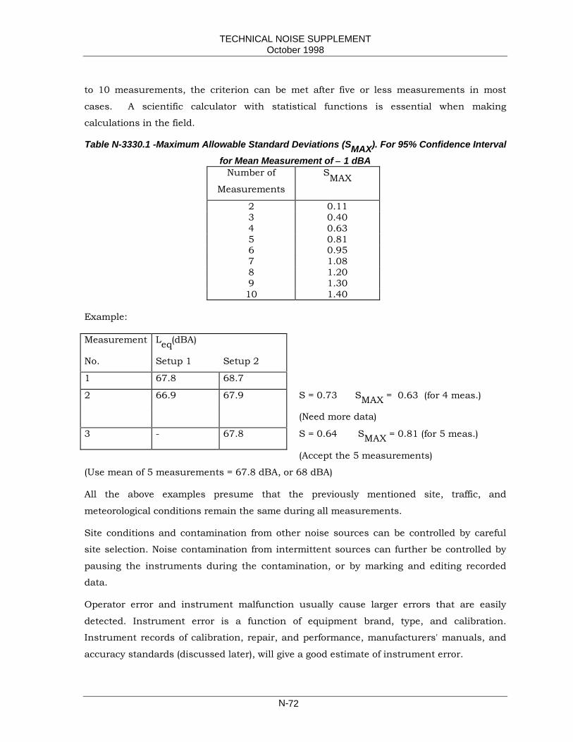
TECHNICAL NOISE SUPPLEMENTOctober 1998
N-72
to 10 measurements, the criterion can be met after five or less measurements in most
cases. A scientific calculator with statistical functions is essential when making
calculations in the field.
Table N-3330.1 -Maximum Allowable Standard Deviations (SMAX). For 95% Confidence Intervalfor Mean Measurement of ± 1 dBA
Number of
Measurements
SMAX
2 0.113 0.404 0.635 0.816 0.957 1.088 1.209 1.30
10 1.40
Example:
Measurement Leq(dBA)
No. Setup 1 Setup 2
1 67.8 68.7
2 66.9 67.9 S = 0.73 SMAX = 0.63 (for 4 meas.)
(Need more data)
3 - 67.8 S = 0.64 SMAX = 0.81 (for 5 meas.)
(Accept the 5 measurements)
(Use mean of 5 measurements = 67.8 dBA, or 68 dBA)
All the above examples presume that the previously mentioned site, traffic, and
meteorological conditions remain the same during all measurements.
Site conditions and contamination from other noise sources can be controlled by careful
site selection. Noise contamination from intermittent sources can further be controlled by
pausing the instruments during the contamination, or by marking and editing recorded
data.
Operator error and instrument malfunction usually cause larger errors that are easily
detected. Instrument error is a function of equipment brand, type, and calibration.
Instrument records of calibration, repair, and performance, manufacturers' manuals, and
accuracy standards (discussed later), will give a good estimate of instrument error.
TECHNICAL NOISE SUPPLEMENTOctober 1998
N-73
Meteorological limits for comparisons of noise measurements will be discussed in section N-
3600, "Environmental Constraints".
The remaining factor to be discussed is traffic. The next topic covers a method of
normalizing noise measurements made under different traffic conditions.
N-3340 Normalizing Measurements for Differences in Traffic Mixes and Volumes
Before applying the criteria discussed in section N-3330, repeated measurements must be
adjusted for differences in traffic mix and volume. The effects of traffic differences can be
calculated by the noise prediction models and compared with the actual differences in the
measurements. However, a simple method to normalize measurements for differences in
traffic mixes and volumes has been developed for optional use in the field.
The method involves field calculations that, with practice, can be carried out in a few
minutes with a log function calculator. The repeated measurements are field adjusted for
the same traffic conditions as the first measurement. The adjusted (normalized)
measurements may then be compared directly according to the criteria in section N-3330.
The obvious advantage of using the field method is that it may eliminate the need for
coming back to the same site at a later date, if repetition criteria are not met.
As is the case with most simplified methods, there are certain limitations to the use of this
field normalization procedure. The method should NOT be used when:
1. Average traffic speeds are not the same for each measurement. (This is difficult toverify, but under free flow conditions at a specific location speeds will generally beconstant within a few mph).
2. Truck speeds are significantly different (more than 5 mph) from auto speeds.
3. Speeds cannot be determined within 5 mph.
4. Ratio of distances from receiver to the center line of far (directional) lane group, andreceiver to center line of near (directional) lane group is greater than 2:1. For most8-lane urban freeways, this means that the receiver should not be closer than 45feet from the edge of the traveled way.
5. Directional split of traffic is different by more than 20% for each vehicle groupbetween measurements. For example, if during the first measurement thedirectional split between heavy trucks is 60/40 and during the next measurement80/20 or 40/60, the method would still be valid. However, if the second split wouldbe 85/15 or 35/65 the method would be inaccurate. This criterion is usually met.
The method uses the concept of Equivalent Vehicles (VE), which equates medium and heavy
trucks to an acoustically equivalent number of autos. Based on California Vehicle Noise
Reference Energy Mean Emission Levels (Calveno REMELs, see Section N-5510) one heavy

TECHNICAL NOISE SUPPLEMENTOctober 1998
N-74
truck traveling at 55 mph makes as much noise as approximately 13 autos cruising at the
same speed. A medium truck at 55 mph is acoustically equivalent to approximately 5
autos passing at the same speed. These heavy truck, medium truck and auto relationships
are speed dependent and are the same for the maximum noise level (LMAX) and time
averaged noise levels (Leq
).
The relationships do not take into consideration source heights and may not be used if the
source to measurement site is intercepted by a barrier or natural terrain feature. Table N-
3340.1 shows Equivalent Vehicles for speeds from 56 km/h (35mph) to 105 km/h (65 mph)
in 5 mph increments, based on Calveno REMELS. Table N-3340.2 shows the same table
based on the new TNM REMELs for baseline conditions. The latter should be used when
the TNM noise prediction model (Section N-5520) is officially implemented.
Table N-3340.1 - Equivalent Vehicles Based on Calveno REMELs*NUMBER OF EQUIVALENT VEHICLES
Speed, km/h (Mph) 1 Heavy Truck = 1 Medium Truck = 1 Automobile =56 (35) 30.9 9.4 164 (40) 24.1 7.8 172 (45) 19.0 6.7 180 (50) 15.3 5.8 1
88.5 (55) 12.8 5.1 197 (60) 10.9 4.7 1
105 (65) 9.5 4.3 1*Based on California Vehicle Noise Reference Energy Mean Emission Levels andvehicle definitions in FHWA-RD-77-108 (Also see sections N-4400 and N-5510)
Table N-3340.2 - Equivalent Vehicles Based on TNM REMELs**NUMBER OF EQUIVALENT VEHICLES
Speed, km/h (mph) 1 Heavy Truck = 1 Medium Truck 1 Automobile =56 (35) 19.1 7.1 164 (40) 15.1 5.8 172 (45) 12.9 5.0 180 (50) 11.5 4.5 188.5 (55) 10.4 4.1 197 (60) 9.6 3.7 1105 (65) 8.9 3.5 1113 (70) 8.3 3.2 1
**Based on FHWA Traffic Noise Model (TNM) Reference Energy Mean EmissionLevels and vehicle definitions in FHWA-PD-96-008, DOT-VNTSC-FHWA-96-2 (Alsosee sections N-4400 and N-5520)
Example of calculating equivalent vehicles using Table N-3340.1:
Given: In 15 minutes the following traffic was counted: 76 heavy trucks, 34 medium trucks,and 789 autos Average traffic speed was 55 mph.
Assignment: Convert traffic counts to Equivalent Vehicles.
Solution: (using Table N-3340.1)
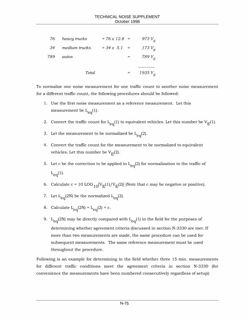
TECHNICAL NOISE SUPPLEMENTOctober 1998
N-75
76 heavy trucks = 76 x 12.8 = 973 VE
34 medium trucks = 34 x 5.1 = 173 VE
789 autos = 789 VE
________
Total = 1935 VE
To normalize one noise measurement for one traffic count to another noise measurement
for a different traffic count, the following procedures should be followed:
1. Use the first noise measurement as a reference measurement. Let this
measurement be Leq(1).
2. Convert the traffic count for Leq(1) to equivalent vehicles. Let this number be VE(1).
3. Let the measurement to be normalized be Leq(2).
4. Convert the traffic count for the measurement to be normalized to equivalent
vehicles. Let this number be VE(2).
5. Let c be the correction to be applied to Leq(2) for normalization to the traffic of
Leq(1).
6. Calculate c = 10 LOG10[VE(1)/VE(2)] (Note that c may be negative or positive).
7. Let Leq(2N) be the normalized Leq(2).
8. Calculate Leq(2N) = Leq(2) + c.
9. Leq(2N) may be directly compared with Leq(1) in the field for the purposes of
determining whether agreement criteria discussed in section N-3330 are met. If
more than two measurements are made, the same procedure can be used for
subsequent measurements. The same reference measurement must be used
throughout the procedure.
Following is an example for determining in the field whether three 15 min. measurements
for different traffic conditions meet the agreement criteria in section N-3330 (for
convenience the measurements have been numbered consecutively regardless of setup):

TECHNICAL NOISE SUPPLEMENTOctober 1998
N-76
15 min Leq
Meas.No.
SetupNo. (dBA)
HeavyTrucks
MediumTrucks Autos Speed
(mph)
EquivalentVehicles
(VE)
1 1 74.4 100 50 1275 55 2810
2 1 75.5 150 100 850 55 3280
3 2 74.0 60 30 1700 55 2621
Correction c for Leq
2 = 10 LOG10 V 1V 2
E
E
= 10 LOG10
28103280
= - 0.7
Leq
2N = Leq
2 + c = 75.5 - 0.7= 74.8 dBA
Correction c for Leq
3 = 10 LOG10 28102621
= + 0.3
Leq
3N = 74.0 + 0.3 = 74.3
Normalized Data, Leq, dBA:
Norm.Meas. Setup L
eq
No.: No.: (dBA)1 1 74.42 1 74.83 2 74.3
Further examination indicates that the agreement criteria of section N-3330 were met, and
no further measurements are necessary.
The actual measurements and traffic counts may now be used back at the office as follows:
Average the energy of the measurements = 74.5 dBA (Report as 75 dBA)
Average the 15-minute traffic counts:
Mean HT's (15 min.) =
100 + 150 + 60
3 = 103.3
Mean MT's (15 min.) =
50 + 100 + 30
3 = 60.0
Mean Autos (15 min.) =
1275 + 850 + 1700
3 = 1275.0
Expand the average 15 minute traffic counts to 1-hour:

TECHNICAL NOISE SUPPLEMENTOctober 1998
N-77
Mean HT's (1-hour) =103.3x 4 = 413
Mean MT's (1-hour) =60.0x 4 = 240
Mean Autos (1-hour) =1275.0x 4 = 5100
The expanded average traffic count may be used in the prediction model to calculate the
noise level. The result may be compared to the energy-averaged measurement. Section N-
5400 explains how this comparison may be used for “calibrating” the prediction model.
Although Tables N-3340.1 and N-3340.2 are based on different REMELS, the results of the
normalization process will not be significantly different using either table. For example,
using the data in the previous example with Table N-3340.2, instead of Table N-3340.1
would yield only slight differences (0.2 dBA) in normalized measurements No.2 and 3, and
the same energy-averaged noise level.
Normalized Data, Leq, dBA:
Norm.Meas. Setup L
eq
No.: No.: (dBA)1 1 74.42 1 75.03 2 74.1
Average the energy of the measurements = 74.5 dBA (Report as 75 dBA).
N-3350 Classroom Noise Measurements
Determining a project’s traffic noise impacts on school classroom interiors (see Section 4.3)
requires taking simultaneous noise measurements inside and outside the classroom to
measure the attenuation provided by the building. While outside noise levels can be
predicted, there are no reliable modeling techniques available for interior noise levels. To
predict an interior noise level, the measured building attenuation may be applied to the
predicted outside level.
If the project involves a reconstruction of an existing freeway, simultaneous traffic noise
measurements may be taken inside and outside the classroom. Microphones should be
placed as shown in Figure N-3350.1 (a) and (b).
Figure N-3350.1(a) shows the preferred setup. Microphone 1 (Mic.1) should be placed
outside the classroom at approximately the same distance from the freeway as the center of
the classroom. Care must be taken to place the microphone far enough away from the
building to a avoid significant shielding by the corner of the building. This can be
accomplished by maintaining at least a 70o angle between a perpendicular line to the

TECHNICAL NOISE SUPPLEMENTOctober 1998
N-78
freeway and a line to the corner of the building (see Figure N-3350.1(a)). Mic. 2 should be
placed in the center of the classroom.
Figure N-3350.1(b) shows an alternate setup, to be used if (a) is not possible. Mic. 1 should
be positioned at least 3 m from the building to avoid noise reflections from the building.
The disadvantage of this setup is that Mic.1 and Mic.2 are not equal in distance from the
freeway. If Mic. 1 is 60 m or more from the freeway, the effects of unequal distances can
usually be ignored. Assuming a 10 m x 10 m classroom the error would be 0.5 dBA or less.
Between 20 and 60 m a distance adjustment of -1 dBA would have to be applied to Mic.1 in
order to normalize Mic. 1 to Mic. 2. If the distance from Mic.1 to the freeway is less than 20
m, a greater adjustment will be necessary. The model (Section 2.4) may be used to
calculate the adjustments.
If the classrooms are not air-conditioned and rely on open windows/doors for ventilation,
the simultaneous measurements should be made both with doors and windows open and
closed conditions. The noise attenuation provided by the building under these conditions is
useful for predicting inside classroom noise levels as well as choosing noise abatement
options if needed. For instance, if a classroom interior is not expected to meet the inside
classroom noise criterion with the windows/doors open, but will meet the criterion with
windows/doors closed, noise abatement considered may include sealing windows, and
adding air-conditioning.
If the project is on a new alignment, there is no existing traffic source that can be used to
measure building attenuation. In that case it is appropriate to use an artificial noise
source (Figure N-3350.2). Acceptable choices would be traffic noise tape recordings or an
electronically generated noise spectrum that approximates typical traffic noise. This
spectrum should be linear, from 31.5 Hz to 500 Hz, and decrease at six decibels per octave
from 500 Hz to 4000 Hz. Amplification should be sufficient to produce A-weighted sound
levels at least 10 dBA above background noise levels at exterior as well as interior locations.
A commercial quality loudspeaker should be used with directional characteristics such that
a 2000 Hz signal measured at 45 degrees from a perpendicular to the face of the speaker is
no more than six decibels below the level measured at the same distance on the
perpendicular axis. The sound level output must be kept constant for inside and outside
measurements.

TECHNICAL NOISE SUPPLEMENTOctober 1998
N-79
Figure N-3350.1 - Classroom Noise Measurements (Reconstruction of Existing Freeway)
Figure N-3350.2 - Classroom Noise Measurements (Project on New Alignment, Using ArtificialSound Source)
F R E E W A Y
70omin.
3 m min.
CLASSROOMS
Mic.1 Mic.2 Mic.2
Mic.1
a) Preferred Setup b) Alternate Setup
D1
D2
45o
Microphone(Center of
Room)
CLASSROOMNOTE: Ratio of D2/D1must be equal to or lessthan 2:1
Loudspeaker

TECHNICAL NOISE SUPPLEMENTOctober 1998
N-80
The loudspeaker is a point source. To account for all the possible angles of incidence
provided by a line source and to avoid reflections from the building face, the speaker should
be positioned as shown in Figure N-3350.2 for the indoor noise measurements.
Avoid placing the speaker and the microphone so that there is a direct line of sight between
the two through an open door or window. If possible, take additional measurements at 15,
30, and 60 degrees and average the results. If only one angle is used, it should be 45
degrees.
For the outdoor noise measurements, the distance from speaker to the outdoor microphone
should be equal to the distance from the speaker to the indoor microphone. Since indoor
and outdoor measurements can not be taken simultaneously, the sound level output of the
artificial source must be the same for inside and outside measurements.
N-3400 INSTRUMENTATIONThe instruments used for measuring or recording noise are available from a wide variety of
manufacturers, models, types, accessories, degrees of accuracy, prices, and levels of
sophistication. It is not the intent of these Technical Analysis Notes to delve into all the
details of noise instruments, nor to endorse certain manufacturers. There are informative
catalogs available from all major manufacturers to help decide which equipment to
purchase, and sales representatives are usually very helpful in demonstrating the
equipment. Once purchased, user's manuals will be useful, ready references for specific
operating procedures.
It is, however, strongly recommended that the NT,M&R be consulted before purchasing
noise instrumentation. NT,M&R calibrates all district noise equipment; compatibility with
its calibration system is essential.
This section will cover general features common to most instruments. The following
categories will be discussed:
1. Sound Level Meters
2. Recording Devices
3. Frequency Analyzers
4. Acoustical Calibrators
5. Meteorological and Other Non-Noise-Related Equipment.

TECHNICAL NOISE SUPPLEMENTOctober 1998
N-81
N-3410 Sound Level Meters (SLM)
The American National Institute of Standards (ANSI) has established requirements for SLM
accuracy in standard ANSI S1.4-1983 (Revision of S1.4-1973) and ANSI S1.4N-1985
Amendment To ANSI S1.4-1983. The standard defines three basic types of SLM:
1. Type 0 - Laboratory Standard (primarily designed for laboratory use)
2. Type 1 - Precision (field use)
3. Type 2 - General Purpose (field use)
The expected total allowable error for a type 1 SLM in the field is +/-1.5 dB; for a type 2
SLM in the field the allowable error is +/- 2.3 dB. These expected values of total allowable
errors apply to an instrument selected at random. These errors may be reduced for a
specific instrument through careful calibration and adjustment.
For each type, the standard requires three frequency weightings, A, B, and C, and two
response settings: slow and fast. In addition, the standard permits other optional features
in an SLM, such as impulse and peak measuring capabilities, wide ranges for the display of
sound level on an analog indicator, digital displays, etc.
Because an SLM may be needed for special purposes that require only part of the basic
type requirements, a meter may be designated type S, followed by the type, and the
available frequency weighting, and/or response setting. Example: type "S2A, fast" is a type
2 SLM with only an "A" weighting network and a "fast" response setting.
The standard also requires the manufacturer to mark the SLM with the type number and
the special purpose (if any).
All SLM used by Caltrans or its contractors shall be of any type described above (types 0, 1,
2 or S with A weighting). The type must be marked on the SLM by the manufacturer.
An older type 3 SLM defined in ANSI S1.4-1971 and S1.4-1971 (R1976) or SLM not marked
with the type shall not be used. Type 3 was discontinued with S1.4-1983.
Although SLM come in many levels of sophistication they all have the following general
components:
1. Microphone System (Microphone and Preamplifier) - The microphone converts air
pressure fluctuations into an electrical signal that is in turn measured by
instrumentation such as the SLM, or a third -octave band spectrum analyzer. Most
microphones can be detached from the SLM body and connected to an extension

TECHNICAL NOISE SUPPLEMENTOctober 1998
N-82
cable. (In order to satisfy a type 0 or 1 requirement the microphone may need to be
separated from the SLM body.)
Microphones come in various diameters. The 1/2 inch diameter microphone is most
commonly used. The air condenser microphone (most common) consists of a
membrane and a back plate, separated by an air gap. The width of the air gap
fluctuates as the membrane vibrates in a sound field, thereby changing the
capacitance. Microphones of SLM complying with the type standards are omni-
directional, have a flat frequency response and are sensitive over a wide range of
frequencies.
A compatible preamplifier, usually manufactured as part of the microphone system
should always be used. A preamplifier provides high-input impedance and constant
low-noise amplification over a wide frequency range. Depending on the type of
microphone, a preamplifier may also provide a polarization voltage to the
microphone.
2. Wind screen - a spherically or cylindrically shaped screen, generally made of open-
celled polyurethane. When placed over the microphone it reduces wind noise (see
section 3600, "Meteorological Constraints" ). The wind screen should always be used
- even in absence of wind - as it helps protect the microphone against dust and/or
mishaps.
3. RMS Detector - converts peak-to-peak signals to an RMS (root mean square) signal.
The RMS measure is derived by first squaring the signal at each instant, obtaining
the average (mean) of the squared values, and taking the square root of this average.
4. Amplifier - amplifies the electrical signal.
5. Frequency weighting filters (A, B, C), as required by ANSI S1.4-1983 and S1.4-1985.
The "A-weighting" is used internationally for environmental noise measurements
(including transportation noise).
6. Slow and/or Fast Response Switch - refers to time averaging characteristics of the
SLM. On the slow setting, the averaging of sound levels takes place over 1 second
increments; on the fast setting the averaging time is 0.125 second. On a real time
display (digital or analog) the sound level fluctuations are easier to read on the slow
setting than in the fast position. The latter, however, gives a better resolution of
instantaneous sound levels.
7. Range Setting - allows setting of the correct range of sound levels to be measured.
TECHNICAL NOISE SUPPLEMENTOctober 1998
N-83
8. Analog or Digital Display - displays instantaneous noise levels and/or integrated
averages. Digital displays often have multi-function switches that allow the user to
view various noise descriptors such as Leq, LMAX etc.
9. Battery Check Switch - allows user to check battery voltage.
10. Output for various recording devices.
11. Power On/Off Switch
Many SLM also have pause switches to interrupt data sampling; preset time switches
allowing sampling over a predesignated time period; reset switches for starting a new
sampling period and other features.
More sophisticated SLM can be mated to external filter sets to allow 1 or 1/3 octave
frequency analysis in the field.
N-3420 Recording Devices
Three main types of recording devices can be connected to most SLM outputs: Graphic
Level Recorders, Audio Tape Recorders, and Microprocessors.
N-3421 Graphic Level Recorder (GLR)
The GLR records sound levels graphically by instantaneous dB vs. time. GLR's provide a
permanent record of fluctuating noise levels over time. Such a record is useful in several
ways:
• The GLR trace provides additional information for time averaged noise levels with
respect to constancy or fluctuation of sound levels. Noise intrusion is a function of
the number and dynamic range of these fluctuations.
• The traces can be effectively used in litigation involving noise. A third, independent
party can analyze the trace and derive various noise descriptors from it.
• The traces can also be used as a backup for noise levels obtained from a visual
display. This guards against errors.
The GLR traces can either be manually or electronically (with a digitizer) reduced to various
noise descriptors at a later date.

TECHNICAL NOISE SUPPLEMENTOctober 1998
N-84
N-3422 Audio Tape Recorders
Audio recording of sound levels for lab analysis at a later time are especially suited for
special studies and research. Tape recordings give the noise analyst a great amount of
freedom to do different types of analysis, using any noise descriptor desired, and various
frequency analyses.
Tape recorders need to be high quality scientific recorders, with flat frequency response and
high signal-to-noise ratios.
N-3423 Microprocessors
Microprocessors can analyze the signals from one or more SLM's simultaneously. The
signals are converted into various noise descriptors, designated by the noise analyst.
Depending on the available software, frequency analysis can also be performed. The
microprocessor is an invaluable tool in research as it enables the researcher to take many
noise measurements simultaneously at different locations.
Microprocessors are usually connected to a printer or plotter for a hard copy of the data
results.
N-3430 Frequency Analyzers
Frequency analyzers are used to study frequency spectrums of sound levels. They are used
more for research than for routine noise analysis. There are two basic types of frequency
analyzers: Real Time Analyzers and Fast Fourier Transform (FFT) Analyzers.
N-3431 Real Time Analyzers
The output of an SLM or tape recorder is fed through a set of filters and decomposed into
frequency ranges of 1 or 1/3 octaves. The term real time refers to the processing and
display of ever changing instantaneous sound spectra. When a tape recorder is used to feed
in the audio signal, frequency spectra at various instants can easily be analyzed by freezing
the spectrum at the exact moments of interest. A typical example might be the frequency
spectra of vehicles passing by an observer, coinciding with the maximum noise levels.
N-3432 Fast Fourier Transform (FFT) Analyzers
The sound signal is processed by using mathematical equations to construct a continuous
frequency power spectrum. The FFT does not produce a 1 or 1/3 octave band analysis. The

TECHNICAL NOISE SUPPLEMENTOctober 1998
N-85
FFT analyzer is a useful tool in sound intensity measurements, requiring specialized
equipment. This is not a tool for routine environmental noise measurements.
N-3440 Acoustical Calibrators
Acoustical calibrators are used to calibrate the SLM/Recorder system in the field. They are
manufactured to fit specific SLM only. The calibrator fits over the top of the microphone
(wind screen removed). Care must be taken that the microphone is properly seated in the
calibrator cavity. When activated the calibrator emits an audio signal at a reference
frequency and decibel level. Most calibrators have a reference level of 94 dB at 1000 Hertz.
The SLM/Recorder system can than be adjusted to this level.
N-3450 Meteorological and Other Non-Noise-Related Equipment
Basic meteorological instruments are necessary to perform measurements for section N-
3600, "Meteorological Constraints".
It is recommended that, at the minimum, the following meteorological equipment be used
simultaneously with noise measurements:
1. Hand-held anemometer which measures wind speed to the nearest mile per hour or
knot up to at least 15 mph, and direction to the nearest 22 1/2 degrees (16 point
compass). Hand held anemometers may be adapted to fit on a tripod for easier use.
2. The anemometer must be oriented to true north with an accurate pocket compass,
adjusted for magnetic declination.
3. Thermometer.
4. Relative Humidity Meter.
Non-essential, but helpful equipment includes a radar gun to measure traffic speeds.
Other recommended items include tape measures, survey levels (or hand levels), and rods
to survey the site and document microphone positions with reference to landmarks, and
watches or stopwatches to time the measurements. Portable radios may be helpful to
maintain contact with traffic counting personnel. Traffic counters are also very useful.

TECHNICAL NOISE SUPPLEMENTOctober 1998
N-86
N-3500 NOISE MEASUREMENT PROCEDURESThis section covers general procedures for routine noise measurements. Manufacturers'
user's manuals should be consulted for operating each specific instrument. The following
procedures are common to all routine Caltrans noise measurements.
N-3510 Instrumentation Setup
The SLM microphone should be placed 5 feet above the ground, and at least 10 feet from
reflecting surfaces, such as buildings, walls, parked vehicles, bill boards, etc. Operators
should be careful not to shield the microphone with their bodies during the measurements.
Other obstructions between microphone and noise source should be avoided, unless they
are representative of the region of interest.
If the microphone is not separated from the SLM body, the SLM should be used with a
tripod. If the microphone is separated from the SLM body, the microphone should be placed
on a tripod or other stand. Test tube clamps are useful for this purpose.
Set up meteorological equipment. Thermometers should be in the shade. Anemometer
should have good exposure to representative winds.
N-3520 Field Calibration
Acoustical calibrators are used to calibrate the SLM/Recorder system in the field. They are
manufactured to fit specific SLM only. The calibrator fits over the top of the microphone
(wind screen removed). Care should be taken that the microphone is properly seated in the
calibrator cavity. When activated the calibrator emits an audio signal at a reference
frequency and decibel level. Most calibrators have a reference level of 94 dB at 1000 Hertz.
Some have a choice of several frequency settings. If the calibrator offers these choices,
1000 Hertz should be used for calibration. The SLM/Recorder system can then be adjusted
to this level. Follow procedures in manufacturers' user's manuals.
SLMs/Recorder system should be calibrated before and after each setup. If several
measurements are made during the same setup, calibration may also be checked between
measurements. For routine measurements, if the SLM reading differs by less than 0.5 dB
from the reference level indicated on the calibrator, the SLM/Recorder system need not be
adjusted. If the SLM reading deviates by 0.5 dB or greater, or if measurements are part of a
special study where extreme accuracy is required, the SLM/Recorder system should be
adjusted within 0.1 dB of the reference level.
TECHNICAL NOISE SUPPLEMENTOctober 1998
N-87
For all measurements, if the final calibration of the acoustic instrumentation differs from
the initial calibration by 1 dB or more, all the data measured with the system between the
calibrations should be discarded and repeated. The instrumentation and connections
should be thoroughly checked before repeating the measurements.
If the final calibration is less than 1 dB from the initial calibration, all data measured with
that system between the initial and final calibration should be adjusted as follows:
Data Adjustment = Calibrator Reference Level - [(CALINITIAL + CALFINAL) / 2].
An example for routine measurements follows:
• Calibrator Reference Level = 94.2 dB
• CALINITIAL = 94.4 dB
• CALFINAL = 94.6 dB
Then: Data Adjustment = 94.2 - [(94.4 + 94.6) / 2] = -0.3 dB.
All data measured in between the two calibrations should be adjusted by -0.3 dB; i.e. a
measurement of 66.7 dBA would become 66.4 dBA. NOTE: For routine measurements it is
customary to round off and report the final adjusted value to the nearest dB. 66.4 dBA
would be reported as 66 dBA, 66.5 dBA as 67 dBA.
The field calibration procedure follows:
1. Allow adequate warm-up of instruments before calibration (at least 1 minute or asspecified in manufacturer's manual). Be sure that all proper connections have beenmade, and batteries are fresh or adequately charged.
2. Calibrator should be carefully placed over the microphone and properly seated. Avoidtouching calibrator during calibration.
3. Use proper screwdriver to make calibration adjustments to the SLM. If a GLR, or otherdevice is used as part of a system the calibration should include the GLR also. TheSLM should be calibrated first, then the GLR.
4. See manufacturer’s user’s manual for particular instructions.
N-3530 Measurements
Following calibration of equipment a wind screen should be placed over the microphone.
Frequency weighting should be set on "A". Set proper response setting at fast or slow.
Whenever possible use fast.
TECHNICAL NOISE SUPPLEMENTOctober 1998
N-88
On more sophisticated SLMs, preset the sampling time, sampling interval, and proper noise
descriptor (Leq
, or in some cases LMAX
).
Set the proper range of noise levels. If unsure, take a short preliminary measurement.
During the noise measurements, note any noise contaminations, such as barking dogs,
local traffic, lawn mowers, aircraft overflights, etc. If SLM is equipped with a Pause or
Standby switch or button, the measurement should be temporarily interrupted until
contamination ceases. Mark contaminated section of GLR trace with pre-assigned codes,
such as "D" for barking dog, "AC" for aircraft, etc.
Avoid talking during measurements. Curious bystanders will often ask the operator what
is going on. A good way to avoid talking near the microphone is to stand 25 to 50 feet from
the microphone, far enough not to contaminate measurement, but close enough to watch
the set up.
If highway noise measurements are taken, traffic should be counted simultaneously with
the noise measurements. As a minimum, directional traffic should be counted separately.
Lane-by-lane traffic counts are best, but often not practical as they are too labor-intensive.
Traffic should be segregated into three vehicle groups: heavy trucks, medium trucks, and
autos. Definitions of these are covered in FHWA-RD-77-108 and in Chapter 4000 Noise
Analysis Procedures. Average speeds for each vehicle group and each direction should be
estimated from either a radar gun (if available) or test runs with a vehicle in the flow of
traffic during the noise measurements.
Wind speed, wind direction, temperature, humidity, and sky conditions (clear, partly
cloudy, overcast, fog, or haze) should be observed and documented.
After the last measurement of the setup, equipment should be recalibrated before turning
power off. Also, any time the power is accidentally or otherwise interrupted during or in
between measurements, instruments need to be recalibrated before taking additional
measurements.
After the last measurement of the setup, equipment should be recalibrated before turning
power off. The procedure for calibration and necessary data adjustment was discussed in
the preceding section N-3520 Field Calibration.
TECHNICAL NOISE SUPPLEMENTOctober 1998
N-89
N-3540 Documentation
Measurement data should be carefully recorded. If the data is read from a display and
hand copied on a form, double-check the readings and, if possible, have another confirm
your record.
It is recommended that blank forms be printed in advance for noise data, meteorological
data, traffic counts, and site data. With the advent of personal computers, the forms can
easily be designed for various types of measurements or specific studies.
The following items should be documented:
1. Noise measurement sites. A sketch showing microphone location in relationship to
natural or artificial land marks. Show distances to the nearest foot to building
corners, trees, street signs, curbs, fences, etc. Include enough detail on the sketch
to enable anyone to reoccupy, at a later date, the three dimensional (including
height above ground) position of the microphone within one foot horizontally and
0.5 foot vertically. Show accurate three dimensional relationships between source
and site. Cross sections should be obtained, either from accurate maps or field
surveys. Sites should also be located on maps showing all receivers used in the
noise analysis. Also include District, County, Route No. And Kilometer Post of site.
2. Noise Measurements. Record all instruments used for the noise measurements,
manufacturers, model numbers, serial numbers. Also important are the calibrator
make, model, serial number, reference level, frequency, and last calibration date.
Show names of instrument operators and persons recording the data. Show before
and after calibration data. Record site number, date, time, length of measurement,
noise descriptor, pertinent settings on SLM/Recorder system, and noise data.
Include remarks, notes of contamination, or anything that might have a possible
effect on the measurement results.
3. Meteorological Conditions. Include prevailing wind direction and speed during the
noise measurements, as well as temperature, relative humidity, and sky conditions.
Indicate approximate height, and location of measurements. Show date, time, site
no., name of observer.
4. Traffic Counts. Show the number of vehicles broken down by classification. It is
important to indicate the location of the traffic counts, no. of lanes or lane groups
counted, direction, length of time, time, District, County, Route, Post Mile, names of
personnel, along with the counts and speeds.

TECHNICAL NOISE SUPPLEMENTOctober 1998
N-90
Usually, four different forms need to be used to accommodate all of the above
documentation. Care must be taken that each form contains enough information to make
necessary cross references between noise measurements, traffic counts, meteorology and
site information.
N-3600 METEOROLOGICAL CONSTRAINTS ON NOISE MEASUREMENTS
There are several ways meteorological conditions can affect noise measurements. Wind
speeds over 5 m/s (11 mph) may at an ambient noise level of 40-45 dBA begin to
contaminate noise measurements with a rumbling noise due to frictional forces on a
microphone covered with a wind screen. Without the screen, the effect would be present at
a much lower wind speed.
Extremes in temperature and relative humidity will affect critical components of sound level
meters. For instance, during conditions of high humidity water condensation can form on
the vibrating microphone membrane causing a “popping” sound which can contaminate
noise measurements.
Rain or snow on highway pavement alter the levels and the frequencies of tire/pavement
noise, causing it to vary in unpredictable ways from noise levels on dry pavements, on
which vehicle noise source characteristics are based.
Refraction caused by wind shear and/or temperature gradients near the ground surface,
will also alter noise levels. The effects of refraction were discussed in section N-2143.
When noise levels are compared to determine the effect(s) of a transportation project on the
noise environment, or to evaluate the effectiveness of a noise abatement measure, the
“before” and “after” noise levels must be for equivalent meteorological conditions.
The following sections include listings of meteorological constraints on noise measurements
and equivalent meteorological conditions.
N-3610 Meteorological Criteria
Noise measurements should NOT be made when one or more of the following meteorological
conditions exist(s):
1. Wind speeds of more than 5 m/s (11 mph) for routine highway noise measurements.
2. Manufacturers' recommendations for acceptable temperature and humidity ranges
for instrument operation are exceeded. Typically, these ranges are from -10oC to

TECHNICAL NOISE SUPPLEMENTOctober 1998
N-91
50oC (14oF to 122oF) for temperature, and 5% to 90% for relative humidity. Heavy
fog conditions usually exceed the 90% relative humidity range.
3. During rain, snow, or wet pavement conditions.
N-3620 Equivalent Meteorological Conditions
Wind effects on noise levels are caused by refraction (or bending) of the noise rays due to
wind shear near the ground. Noise rays are bent upward upwind, and downward downwind
from the source. The result is the decrease of noise upwind and increase of noise
downwind from a source.
Recent studies by Caltrans N.T.M.&R. and others have shown that this wind effect can
affect noise measurements significantly even at relatively close distances to noise sources.
Section N-3330 indicates that, in order to compare noise measurements for agreement, all
site, traffic, and meteorological conditions must be the same.
Noise measurement comparisons can therefore only be made for similar meteorological
conditions. ANSI S12.8 - 1987 "Methods for Determination of Insertion Loss of Outdoor
Noise Barriers" recommends that meteorological equivalence be based on wind,
temperature and cloud cover. The latest revison of the 1987 standard will (as of this writing
in 1998) be published in the near future. The revision recommends the following criteria
for atmospheric equivalence average wind velocities from the source position to the receiver
position. In the case of highway noise, the wind component of interest is perpendicular to
the highway. The standards recommended by the ANSI may be used to define
meteorological equivalency for the purposes of section N-3330, or any time BEFORE and
AFTER noise measurements are performed on noise barriers.
Equivalent Wind Conditions - Wind conditions are equivalent for noise measurements if the
wind class (defined in Table N-3600.1) remains unchanged AND the vector components of
the average wind velocity from the source to receiver (perpendicular to the highway) do not
differ by more than a certain limit. This limit depends on the accuracy desired and the
distance from sound source to receiver. To keep the measurement accuracy due to
atmospheric wind conditions to within ± 1dB, for distances less than 70 m (230 ft), this
limit should be 1 m/s (2.2 mph). If it is desired to keep this accuracy within ± 0.5 dB for
the same distance, the measurements to be compared should each be repeated at least four
times. The 1 m/s limit does not apply to the Calm condition. By convention, the
perpendicular wind component blowing from highway to receiver (microphone position) is
positive (+) while the same component blowing from receiver to the highway is negative (-).

TECHNICAL NOISE SUPPLEMENTOctober 1998
N-92
Table N-3600.1 - Classes of Wind Conditions
WIND CLASS VECTOR COMPONENT OF WIND
VELOCITY, m/s (mph)
Upwind -1 to -5 (-2.2 to -11)
Calm -1 to +1 (-2.2 to +2.2)
Downwind +1 to +5 (+2.2 to +11)
For example, two measurements may be compared when their respective wind components
are 0 m/s and -1 m/s, -1 m/s and -2 m/s, -2.5 m/s and -3.5 m/s, etc, but not when their
respective components are 0.5 m/s and 1.5 m/s (due to the change in wind class).
For purposes of comparison with the Traffic Noise Model, which has no provisions for wind
inputs and therefore predicts noise levels for calm (zero wind) conditions, the perpendicular
wind component needs to be between -1 m/s and +1 m/s (-2.2 mph and +2.2 mph.
Note that the actual wind velocity (direction and speed) needs to be resolved into two
components with directions parallel and perpendicular to the highway. Then, only the
perpendicular component is considered (as long as the actual wind speed does not exceed 5
m/s (11 mph), any wind velocity may be resolved in this manner).
The component of wind velocity for a given set of acoustical measurements should be
determined by:
1. monitoring wind velocity (speed and direction) throughout any period of acoustical
measurements;
2. noting the average speed and direction; and
3. computing from these averages the vector component of wind velocity from the
source to receiver (perpendicular to the highway)
Equivalent Temperature and Cloud Cover - Measurements to be compared (such as before
and after noise barrier measurements, or repeat measurements) should be made for the
same class of cloud cover, as determined from Table N-3600.2, and with the average air
temperatures within 14o C (25o F) of each other.
Equivalent Humidity - Although there are no strict guidelines for equivalence of humidity,
an attempt should be made to pair measurements for similar conditions of humidity, i.e.
avoid comparisons of measurements made under extremely dry conditions (e.g. < 25%) with
those made during humid conditions (e.g. >75%).

TECHNICAL NOISE SUPPLEMENTOctober 1998
N-93
Table N-3600.2 - Cloud Cover Classes
CLASS DESCRIPTION
1 Heavily overcast
2 Lightly overcast (either with continuoussun or the sun obscured intermittentlyby clouds 20% to 80% of the time)
3 Sunny (sun essentially unobscured byclouds at least 80% of the time)
4 Clear night (less than 50% cloud cover)
5 Overcast night (50% or more cloud)cover)
N-3700 QUALITY ASSURANCEAll SLM should be calibrated by, and at the interval recommended by the manufacture, or
by a laboratory accredited to perform calibrations on specified instruments. All calibrations
should be traceable to the National Institute of Standards and Technology (NIST) in
Washington, DC.


TECHNICAL NOISE SUPPLEMENTOctober 1998
N-95
N-4000 TRAFFIC NOISE IMPACT SCREENINGPROCEDURE
This procedure has been developed to aid in determining whether or not a potential for
a traffic noise impact will exist with a proposed Type I highway project defined in the
Traffic Noise Analysis Protocol Section 2.1. If the project passes the screening
procedure, prudent engineering judgment should still be exercised to determine
whether a detailed noise analysis is warranted. If the project is controversial,
sensitive, or when net results of the effects of topography and shielding are complex
and ambiguous, a detailed analysis is recommended (See Sections N-5000 and N-
6000). If the project fails the screening procedure, a detailed noise analysis should be
performed.
A “Noise Analysis Screening Procedure Checklist”, shown in section N-4500 (Figure N-
4500-1), is included for the user’s convenience.
N-4100 SCREENING PROCEDURE STEPS
Following are the steps of the procedure (refer to definitions of italicized words and
phrases in section N-4200 “Definitions for Screening Procedure”).
1) If there are no potentially impacted receivers in the vicinity of the project, thisscreening procedure will be considered passed. If there are potentially impactedreceivers in the vicinity of the project, the conditions in the following stepsshould be satisfied. Failure of one condition constitutes failure of thisscreening procedure, and the detailed analyses in Sections N-5000 and N-6000are recommended.
2) The proposed project should be along an alignment or a realignment of anexisting facility. Potential noise impacts along new alignments are bestinvestigated by a detailed analysis.
3) Shielding conditions, if any, should be equal or improved for the after projectcritical receiver(s) in comparison with those for the same receiver(s) before theproject.
4) Measure existing worst hour noise level(s) at the critical receiver(s).
5) If the existing worst hourly noise is above a level that is 5 dBA below the NAC(e.g. Leq(h) above 62 dBA for land use category B), stop this screeningprocedure; a noise analysis should be performed according to the procedurescovered in Appendix B. If the existing noise level(s) at the most criticalreceiver(s) is (are) 5 dBA or more below the NAC, continue with step (6).
6) The following equation in terms of existing and future hourly equivalent vehiclesand equivalent lane distances should yield a value of less than 3.0 dBA:

TECHNICAL NOISE SUPPLEMENTOctober 1998
N-96
10 1510 10Log
VV
LogDD
E FUTURE
E EXISTING
E EXISTING
E F U TU R E[ ] [ ]( )
( )
( )
( )+ < 3.0 dBA
Where: VE(FUTURE) = Number of Equivalent Vehicles per hour after the
project.VE(EXISTING) = Number of Equivalent Vehicles per hour before the
project.DE(EXISTING) = Equivalent Lane Distance before project.
DE(FUTURE) = Equivalent Lane Distance after project.
7) If the above value is less than 3.0 dBA the project passes the screeningprocedure.
8) If the above value is equal to or greater than 3.0 dBA the project does notpass the screening procedure.
(See section N-4300 “Method of Calculating Equivalent Lane Distance” todetermine DE, and section N-4400 “Method of Calculating Equivalent Vehicles”to determine VE).
Note: Due to the approximation of the coefficient “15” in the above equation,the ratio DE(EXISTING)/DE(FUTURE) should not exceed 4. If it does, it isrecommended that a detailed technical noise analysis be performed.
N-4200 DEFINITIONS FOR SCREENING PROCEDUREFor the purpose of the screening procedure, the following definitions (in alphabetical
order) apply:
Critical Receiver(s) - Potentially impacted receiver(s) where the worst noise impacts (ifany) would occur. Critical receivers are potentially impacted receivers where theafter project noise level or increase is expected to be the greatest.
Equivalent Lane - (See “Method of Calculating Equivalent Lane Distances”, Sec. N-4300) - An imaginary single lane that acoustically represents a multi-lane highway.An Equivalent Lane contains the total traffic volumes present on the highway.
Equivalent Lane Distance - (“See “Method of Calculating Equivalent Lane Distances”,Sec. N-4300) - Distance from the receiver to an Equivalent Lane.
Equivalent Vehicle - (See Method of Calculating Equivalent Vehicles, Sec. N-4400) - Abasic noise source unit that expresses the noise level emitted by heavy trucks andmedium trucks in terms of the equivalent noise level emitted by a certain numberof automobiles. This number is speed-dependent. For example, at 88.5 km/h 1heavy truck produces the same noise level as 13 automobiles; at 56 km/h thenoise level is that of 31 automobiles. The term equivalent vehicle (VE) issynonymous with automobile, but should be used when a vehicle mix normalizedto automobiles is implied. Definitions of heavy trucks, medium trucks andautomobiles are the same as those used in the FHWA Highway Traffic NoisePrediction Model (Report No. FHWA-RD-77-108).
Noise Sources - The existing or future traffic along the before or after projectalignment.
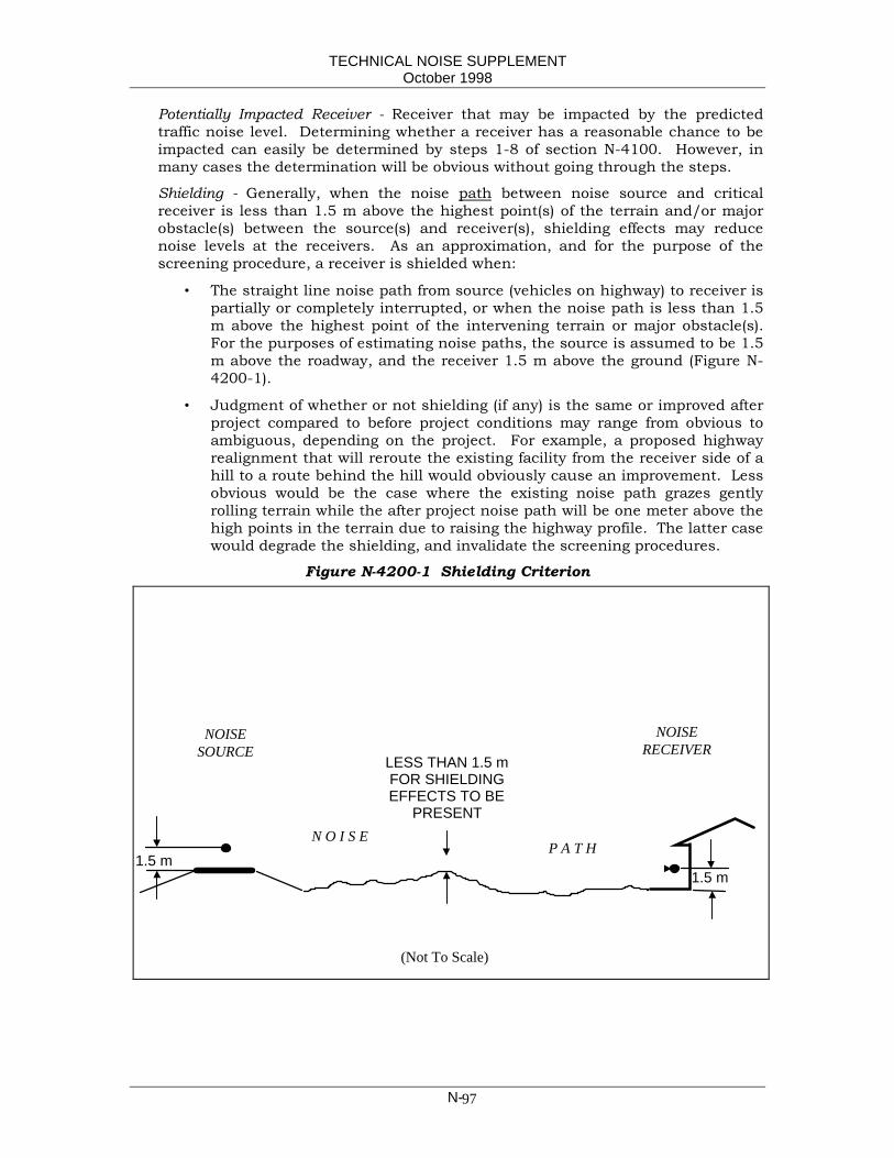
TECHNICAL NOISE SUPPLEMENTOctober 1998
N-97
Potentially Impacted Receiver - Receiver that may be impacted by the predictedtraffic noise level. Determining whether a receiver has a reasonable chance to beimpacted can easily be determined by steps 1-8 of section N-4100. However, inmany cases the determination will be obvious without going through the steps.
Shielding - Generally, when the noise path between noise source and criticalreceiver is less than 1.5 m above the highest point(s) of the terrain and/or majorobstacle(s) between the source(s) and receiver(s), shielding effects may reducenoise levels at the receivers. As an approximation, and for the purpose of thescreening procedure, a receiver is shielded when:
• The straight line noise path from source (vehicles on highway) to receiver ispartially or completely interrupted, or when the noise path is less than 1.5m above the highest point of the intervening terrain or major obstacle(s).For the purposes of estimating noise paths, the source is assumed to be 1.5m above the roadway, and the receiver 1.5 m above the ground (Figure N-4200-1).
• Judgment of whether or not shielding (if any) is the same or improved afterproject compared to before project conditions may range from obvious toambiguous, depending on the project. For example, a proposed highwayrealignment that will reroute the existing facility from the receiver side of ahill to a route behind the hill would obviously cause an improvement. Lessobvious would be the case where the existing noise path grazes gentlyrolling terrain while the after project noise path will be one meter above thehigh points in the terrain due to raising the highway profile. The latter casewould degrade the shielding, and invalidate the screening procedures.
Figure N-4200-1 Shielding Criterion
1.5 m1.5 m
LESS THAN 1.5 mFOR SHIELDINGEFFECTS TO BE
PRESENT
NOISESOURCE
NOISERECEIVER
N O I S EP A T H
(Not To Scale)

TECHNICAL NOISE SUPPLEMENTOctober 1998
N-98
N-4300 METHOD OF CALCULATING EQUIVALENT LANEDISTANCE
The concept of equivalent lane distance is discussed in detail in FHWA-RD-77-108,
“FHWA Highway Traffic Noise Prediction Model”. The FHWA Model allows traffic to be
segregated lane-by-lane, the center line of each lane being associated with a different
source-to-receiver distance. Normally, traffic data is not available lane-by-lane, but
rather by direction, e.g. eastbound (E/B) and westbound (W/B). The normal procedure
is to use the centerline of the directional lanes grouped together, approximating an
acoustical representation of two source locations (e.g. centerline E/B and centerline
W/B). Instead of using the centerline distances however, it is more accurate to use
the equivalent lane distance (DE) as determined by the formula shown in Figure N-
4300-1.
This screening procedure recommends a further simplification by grouping all lanes
(both directions) together and using a single DE , calculated from the source-to-
centerline distances of the nearest and farthest lanes. This method assumes more or
less balanced directional traffic flows and normal medians. If such is not the case, the
method may still be used if traffic flows will have roughly the same (unbalanced)
directional flow ratio with or without the project, and changes in source-to-receiver
distances are not excessive.
Figure N-4300.1 - Equivalent Lane Distance.
DN
DF
CL Far Lane
CL Near Lane
DED
Equivalent Lane Distance, DE
DE = √(DN X DF)
Receiver
Equivalent Lane

TECHNICAL NOISE SUPPLEMENTOctober 1998
N-99
Example of Equivalent Lane Distance Calculation:
Given: an eight-lane freeway with a 6.6 m median. The distance from the receiver to thecenter line of the near lane ( DN ) is 35 m. The distance to the center line of the far lane (DF ) is 66.8 m. What is the Equivalent lane distance ( DE )?
Solution: DE = (DN x DE)0.5 = (35 x 66.8)0.5 = 48.4 m
Notes:• When using one Equivalent Lane Distance for an entire freeway, the total
hourly traffic volumes (in terms of Equivalent Vehicles) of that freeway shouldbe used with the Equivalent Lane Distance.
• Equivalent Lane Distances may be derived from the two centerlines ofdirectional lanes, or from the single nearest lane and farthest lane on theopposite side.
N-4400 METHOD OF CALCULATING NUMBER OFEQUIVALENT VEHICLES
The following method, using either Table N-4400.1 or both Tables N-4400.1 and N-
4400.2 is used to calculate equivalent vehicles (VE). The method essentially
normalizes heavy trucks, medium trucks and autos, to one vehicle group (VE), on the
basis of their acoustical energy. The auto is used as a reference (1 Auto = 1 VE).
Table N-4400.1 may be used by itself if traffic speeds of all vehicles are assumed to
have the same speed, and there is no difference between with and without project
speeds.
Table N-4400.1 - No. of Equivalent Vehicles as a Function of Vehicle Type andSpeed Based on California Vehicle Noise Reference Energy Mean Emission
Levels (Calveno REMELs)*(see Sec. N-5510).
Speed, km/h (mph) 1 Heavy Truck= No. of VE
1 Medium Truck= No. of VE
1 Auto= No. of VE
56 (35) 30.9 9.4 164 (40) 24.1 7.8 172 (45) 19.0 6.7 180 (50) 15.3 5.8 188.5 (55) 12.8 5.1 197 (60) 10.9 4.7 1105 (65) 9.5 4.3 1
Note:

TECHNICAL NOISE SUPPLEMENTOctober 1998
N-100
* This table must only be used while the FHWA-RD-77-108 prediction method isstill in force (see Section N-5510). It must not be used after the predictionmethod is replaced by the new FHWA TNM . (see Table N-4400.3)
Example of Equivalent Vehicle calculation using Table N-4400.1:
Given: an hourly vehicle volume of 5000 autos, 175 medium trucks (MT), and 325 heavytrucks (HT). The traffic speed is 88.5 km/h (55 mph). Convert this volume to number ofVE.Solution: 5000 autos = 5000 x 1 =5000 VE
175 MT = 175 x 5.1 = 893 VE 325 HT = 325 x 12.8 =4160 VE
Total VE = 10053 VE
If speeds of autos, medium trucks and heavy trucks are different, or when with andwithout project noise comparisons are made for different speeds, an additional speedcorrection factor must be applied. The correction for speeds involves multiplying theVE of each of the three vehicle types at the indicated speeds, with a sound energy ratiorelative to the noise level, Leq(h), dBA of a pass by of 1 auto at 15 m (50 ft), traveling at88.5 km/h (55 mph). The number of the VE is thus normalized to a reference speed of88.5 km/h (55 mph), and since the VE is in terms of autos, the energy ratio valueswere derived from Calveno curves for autos. In the following Table N-4400.2 theconversion of instantaneous noise levels to Leq(h) was accounted for in the energyratios by including the traffic flow adjustments per FHWA-RD-77-108.
Table 4400.2 - Speed Corrections For Equivalent Vehicles Based on CaliforniaVehicle Noise Reference Energy Mean Emission Levels (Calveno REMELs)*
(see Sec. N-5510).Speed, km/h (mph) Noise Level of 1
Auto at 15 m (50ft), Leq(h), dBA *
Energy ratio **
56 (35) 34.4 0.2764 (40) 36.1 0.4072 (45) 37.5 0.5580 (50) 38.9 0.7688.5 (55) 40.1 1.0097 (60) 41.1 1.26105 (65) 42.1 1.58
Notes:
* This table must only be used while the FHWA-RD-77-108 prediction method isstill in force (see Section N-5510). It must not be used after the predictionmethod is replaced by the new FHWA TNM (see Table N-4400.4).
** Energy Ratio values were derived from the Calveno Emission Levels for autoswith reference to 88.5 km/h (55 mph) speed and traffic flow adjustment perFHWA-RD-77-108.
Example of using number of equivalent vehicles in Table N-4400.1 and speedcorrections in Table N-4400.2:

TECHNICAL NOISE SUPPLEMENTOctober 1998
N-101
Given: an hourly vehicle volume of 3000 autos at 105 km/h (65 mph), 150 medium trucks(MT) at 97 km/h (60 mph), and 325 heavy trucks (HT) at 80 km/h (50 mph). Convert thisvolume to number of VE.:Solution: 3000 autos = 3000 x 1 x 1.58 = 4740 VE
150 MT = 150 x 4.7 x 1.26 = 888 VE 325 HT = 325 x 15.3 x 0.76 = 3779 VE
Total VE = 9407 VE
When the new FHWA Traffic Noise Model (TNM) is officially mandated for use inCalifornia, Tables N-4400.3 and N-4400.4 will need to be used. These are based onFHWA-PD-96-010; DOT-VNTSC-FHWA 98-2 and FHWA-PD-96-008; DOT-VNTSC-FHWA-96-2.
Table N-4400.3 - No. of Equivalent Vehicles as a Function of Vehicle Type andSpeed Based on TNM Reference Energy Mean Emission Levels (TNM REMELs)*
(see Section N-5520).Speed, km/h (mph) 1 Heavy Truck
= No. of VE1 Medium Truck
= No. of VE1 Auto
= No. of VE56 (35) 19.1 7.1 164 (40) 15.1 5.8 172 (45) 12.9 5.0 180 (50) 11.5 4.5 188.5 (55) 10.4 4.1 197 (60) 9.6 3.7 1105 (65) 8.9 3.5 1113 (70) 8.3 3.2 1
Note:* This table must only be used when the new FHWA TNM noise predictionmodel is in force.
Example of Equivalent Vehicle calculation using Table N-4400.3:
Given: an hourly vehicle volume of 5000 autos, 175 medium trucks (MT), and 325 heavytrucks (HT). The traffic speed is 88.5 km/h (55 mph). Convert this volume to number ofVE.
Solution: 5000 autos = 5000 x 1 =5000 VE 175 MT = 175 x 4.1 = 718 VE 325 HT = 325 x 10.4 =3380 VE
Total VE = 9098 VE
Table N-4400.4 - Speed Corrections For Equivalent Vehicles Speed CorrectionsFor Equivalent Vehicles Based on (TNM REMELs)
(see Section N-5520).Speed, km/h (mph) Noise Level of 1
Auto at 15 m (50ft), Leq(h), dBA *
Energy Ratio**
56 (35) 35.0 0.2564 (40) 36.8 0.37

TECHNICAL NOISE SUPPLEMENTOctober 1998
N-102
72 (45) 38.4 0.5480 (50) 39.8 0.7488.5 (55) 41.1 1.0097 (60) 42.3 1.32105 (65) 43.4 1.70113 (70) 44.5 2.19
Notes:
* This table must only be used when the new FHWA TNM noise predictionmodel is in force.
** Energy Ratio values were derived from the TNM Emission Levels for autos withreference to 88.5 km/h (55 mph) speed and traffic flow adjustment per FHWA-PD-96-010; DOT-VNTSC-FHWA 98-2 and FHWA-PD-96-008; DOT-VNTSC-FHWA-96-2.
Example of using speed corrections:
Given: an hourly vehicle volume of 3000 autos at 105 km/h (65 mph), 150 medium trucks(MT) at 97 km/h (60 mph), and 325 heavy trucks (HT) at 80 km/h (50 mph). Convert thisvolume to number of VE.
Solution: 3000 autos = 3000 x 1 x 1.70 = 5100 VE 150 MT = 150 x 3.7 x 1.32 = 733 VE 325 HT = 325 x 11.5 x 0.74 = 2766 VE
Total VE = 8599 VE
N-4500 NOISE ANALYSIS SCREENING PROCEDURECHECKLIST
The following check list format shown on the next two pages may be used forconvenience of the user of the screening procedure.
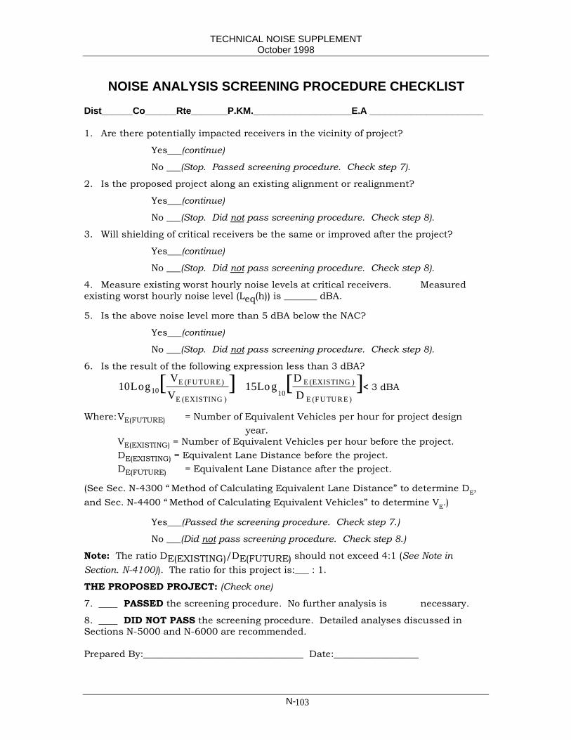
TECHNICAL NOISE SUPPLEMENTOctober 1998
N-103
NOISE ANALYSIS SCREENING PROCEDURE CHECKLIST
Dist______Co______Rte_______P.KM.___________________E.A ______________________
1. Are there potentially impacted receivers in the vicinity of project?
Yes___(continue)
No ___(Stop. Passed screening procedure. Check step 7).
2. Is the proposed project along an existing alignment or realignment?
Yes___(continue)
No ___(Stop. Did not pass screening procedure. Check step 8).
3. Will shielding of critical receivers be the same or improved after the project?
Yes___(continue)
No ___(Stop. Did not pass screening procedure. Check step 8).
4. Measure existing worst hourly noise levels at critical receivers. Measuredexisting worst hourly noise level (Leq(h)) is _______ dBA.
5. Is the above noise level more than 5 dBA below the NAC?
Yes___(continue)
No ___(Stop. Did not pass screening procedure. Check step 8).
6. Is the result of the following expression less than 3 dBA?
10 1510 10Log
VV
LogDD
E FUTURE
E EXISTING
E EXISTING
E F U TU R E[ ] [ ]( )
( )
( )
( )+ < 3 dBA
Where:VE(FUTURE) = Number of Equivalent Vehicles per hour for project designyear.
VE(EXISTING) = Number of Equivalent Vehicles per hour before the project.DE(EXISTING) = Equivalent Lane Distance before the project.DE(FUTURE) = Equivalent Lane Distance after the project.
(See Sec. N-4300 “Method of Calculating Equivalent Lane Distance” to determine DE,and Sec. N-4400 “Method of Calculating Equivalent Vehicles” to determine VE.)
Yes___(Passed the screening procedure. Check step 7.)
No ___(Did not pass screening procedure. Check step 8.)
Note: The ratio DE(EXISTING)/DE(FUTURE) should not exceed 4:1 (See Note inSection. N-4100)). The ratio for this project is:___ : 1.
THE PROPOSED PROJECT: (Check one)
7. ____ PASSED the screening procedure. No further analysis is necessary.
8. ____ DID NOT PASS the screening procedure. Detailed analyses discussed inSections N-5000 and N-6000 are recommended.
Prepared By:__________________________________ Date:__________________

TECHNICAL NOISE SUPPLEMENTOctober 1998
N-104

TECHNICAL NOISE SUPPLEMENTOctober 1998
N- 105
N-5000 DETAILED ANALYSIS - TRAFFIC NOISEIMPACTS
If the project fails the screening procedure discussed in Section 2.2 of the Protocol and
Section N-4000, or if the other conditions discussed in Section 2.2 apply, a detailed traffic
noise impact analysis must be performed. The procedures in this section comply with
analysis requirements of 23 CFR 772, and are consistent with standard acoustical
practices and reasonable engineering judgment.
N-5100 GATHERING INFORMATIONThe first step in a technical noise analysis is to determine how detailed the study needs to
be. This understandably depends on the size and nature of the project. Generally, as the
size of the project, complexity of terrain, and the population density increases, so does the
amount of information and level of effort needed for an adequate noise analysis.
For the analysis, it is necessary to obtain adequate information and mapping showing
project alternates and their spatial relationships to potentially noise sensitive areas. The
“No-Build” alternate should be included. Early in the project, final design details usually
are not yet available and additional analyses may have to be performed as more details are
introduced. Topographical information may also be sketchy in early stages. Field reviews
and recent aerial photographs may be necessary to augment information shown on maps.
Design year traffic information for all project alternates is also necessary.
N-5200 IDENTIFYING EXISTING AND FUTURE LAND-USEAND APPLICABLE NOISE ABATEMENT CRITERIAExisting and reasonably expected future activities on all lands that may be affected by
noise from the highway must be identified (see Section 2.3(a) of the Traffic Noise Analysis
Protocol). Identify existing activities, developed lands, and undeveloped lands for which
development is planned, designed and programmed, which may be affected by noise from
the highway. Development is considered planned, designed and programmed, if a noise
sensitive land-use (subdivisions, residences, schools, churches, hospitals, libraries, etc.)
has received final development approval (generally the issuance of a building permit) from
the local agency with jurisdiction. This information is essential to assess which Noise
Abatement Criteria (NAC) apply for determining traffic noise impacts (see Section 2.4.2 and
Table 2-1 in the Traffic Noise Analysis Protocol). For convenience, the NAC are shown
again in Table N-5200-1.

TECHNICAL NOISE SUPPLEMENTOctober 1998
N- 106
Table N-5200-1. Activity Categories and Noise Abatement Criteria (NAC)
ActivityCategory
NAC,Hourly A-
Weighted NoiseLevel, dBA Leq(h)
Description of Activities
A 57Exterior
Lands on which serenity and quietare of extraordinary significance andserve an important public need andwhere the preservation of thosequalities is essential if the area is tocontinue to serve its intendedpurpose.
B 67Exterior
Picnic areas, recreation areas,playgrounds, active sport areas,parks, residences, motels, hotels,schools, churches, libraries, andhospitals.
C 72Exterior
Developed lands, properties, oractivities not included in Categories Aor B above.
D -- Undeveloped lands.
E 52Interior
Residences, motels, hotels, publicmeeting rooms, schools, churches,libraries, hospitals, and auditoriums.
N-5300 DETERMINING EXISTING NOISE LEVELSExisting noise levels may be determined at discrete locations in the project area, by either
actual noise measurement (see TeNS N-3000), using the traffic noise prediction model
(TeNS N-5510 and N-5520), or a combination of both. The latter is usually the case. This
section discusses how to select these locations, the methods used to determine existing
noise levels, and, where appropriate, to “calibrate” the noise prediction model with
measurements.
N-5310 Selecting Noise Receivers and Noise Measurement Sites
For the purposes of noise analysis a noise receiver is any location included in the noise
analysis. A noise measurement site is a location where noise measurements are taken to
determine existing noise levels, and verify or calibrate the noise prediction model.
Receivers and noise measurement sites may or may not coincide. Normally, there are more
receivers than noise measurement sites, especially when the project involves reconstruction
of existing facilities. In such situations, existing noise levels at receivers are first
determined using the noise prediction model, then verified or calibrated with field

TECHNICAL NOISE SUPPLEMENTOctober 1998
N- 107
measurements at a fewer number of representative sites. It is far less expensive to model
(calculate) noise levels for receivers, than to take noise measurements in the field.
N-5311 ReceiversWithin the identified land-use activity categories adjacent to the project typically lie
numerous noise receivers that need to be examined for future noise impacts. It is not
reasonable, or possible, to examine the impacts at all these receivers. Receivers should
therefore be carefully selected for the noise analysis on the basis of their acoustical
representativeness.
Following are some general recommendations for selecting receivers:
a) Select receivers generally in locations that are now receiving, or are expected to receivethe highest noise levels over the period covered by the analysis. Since, in most cases,impacts will be at receivers closest to the highway, the vast majority of receivers shouldbe in the first row of residences relative to the project alternative. Some commonexceptions include:
1) Projects where realignment would move the noise sources toward receivers otherthan those adjacent to the existing alignment;
2) Projects involving geometry where the first row of homes is partially shielded andthe second row homes may actually receive higher noise levels, for exampleroadways on high embankments;
3) Areas near the ends of proposed barriers where second or third row receptor sitesmay be needed to better define the barrier limits;
4) Projects that involve widening where additional R/W requirements may clear thefirst row of residences and turn the second row into the first.
b) Coincide a noise measurement site with a receiver, whenever possible. However, thismay often not be the case. The selected receiver may not be a good or accessiblelocation for setting up a sound level meter. In that case, a noise measurement siteacoustically representative of the receiver should be selected in a more accessiblelocation.
c) Include other noise-sensitive locations, such as libraries, churches, hospitals, schools,etc.
d) Choose receivers that are acoustically equivalent of the area of concern. The concept ofacoustical equivalence incorporates equivalencies in noise sources (traffic), highwaycross sections, distance from the highway, topography of intervening terrain, shielding,and other pertinent factors. The region under study may need to be subdivided intosubregions in which acoustical equivalence can generally be maintained. One or moreof the previously mentioned acoustical factors should dictate boundaries of eachsubregion. The size of subregions may vary depending on the scope of the project.
e) Select a minimum of two receivers for each acoustically equivalent region or subregion.The actual number necessary to define noise impacts depends not only on the type ofproject but also on such influences as the complexity of highway profile and thevariability of the surrounding terrain. A highway with a straight grade or very shallowvertical curves in a relatively flat area with tract-type residential development thatparallels the highway may need only a couple of receivers to adequately define the noiseimpacts. On the other hand, a project involving a major freeway that includes

TECHNICAL NOISE SUPPLEMENTOctober 1998
N- 108
interchanges, cuts and fills in an area of rolling terrain and non-tract mixed residentialand commercial development will likely need more receivers.
f) Receivers are 1.5 m above the ground elevation, unless dictated by unusualcircumstances, special studies, or other requirements. Exceptions would includeplacing a receiver 1.5 m above a wooden deck of a house situated on a steep slope,instead of 1.5 m above the ground. Similar situations might be encountered withhouses built on top of garages, where second story levels would be more logical receiverlocations. Generally, second story levels are not used as receivers, because exterioruses are negligible and the additional cost of attenuation is high.
g) Select receivers in areas of frequent human use. There is little need to address thenoise impacts of areas where people do not spend much time (for example, parkinglots).
h) To determine the amount of benefited receivers (defined as those predicted to receive atleast 5 dBA noise reduction from noise abatement under consideration), it is oftennecessary to include receivers at the first, second, and third tiers of residences orbeyond in the noise analysis.
N-5312 Noise Measurement SitesThe selection of noise measurement locations requires planning and foresight by the noise
analyst. A fine balance should be achieved between a sufficient number of quality locations
on one side, and the cost and availability of resources on the other.
Preliminary design maps, cross sections, aerial photographs, and field survey data are all
helpful sources of information for selecting noise measurement sites; however, the sites
should be selected only after a thorough field review of the project area.
Following are some recommended site characteristics common to all outside noise
measurement sites:
a) Sites should be clear of major obstructions; reflecting surfaces such as walls ofresidences should be more than 3 m from the microphone positions.
b) Sites should be free of noise contamination by sources other than those of interest.Avoid sites located near barking dogs, lawn mowers, pool pumps, air conditioners, etc.,unless it is the express intent to measure noise from these sources.
c) Sites should be acoustically representative of areas and conditions of interest. Theyshould either be located at, or represent locations of frequent human use.
In addition to the above general site requirements the selection of noise measurement sites
is governed by the same general guidelines as those for selection of receivers in Section N-
5311. Of particular importance is the concept of acoustical equivalence for
representativeness of the area of concern.
More detailed considerations are discussed in the Technical Noise Supplement Section N-
3200.
TECHNICAL NOISE SUPPLEMENTOctober 1998
N- 109
N-5320 Measuring Existing Noise LevelsWhen possible, existing noise levels should be determined by field measurements. As is the
case with all fieldwork, quality noise measurements are relatively expensive. They take
time, personnel and equipment. The noise analyst should therefore carefully plan the
locations, times, duration and number of repetitions of the measurements before taking the
measurements. Meteorological (atmospheric) and other environmental conditions can
significantly affect noise measurements. Particular attention should be given to the
meteorological and environmental constraints described in the Technical Noise Supplement
Section N-3600.
In the noise analysis for a project, the noise measurements are used both to determine
existing ambient and background noise levels, and to calibrate the noise prediction model
when appropriate. Section N-3000 contains details of noise measurements and should be
referred to.
N-5330 Modeling Existing Noise Levels
Noise levels near existing facilities can also be determined by modeling. Although
measurements are preferred, adverse environmental conditions, construction,
unavailability of good measurement sites, or lack of time may make it necessary to
calculate existing noise levels, using the appropriate traffic noise prediction model (s)
described in Section N-5500. However, this can only be done in areas where a defined
highway source exists with minimal surface grid traffic or other contaminating noise
sources.
Often, a combination of measurements and modeling at various receivers is used to
determine existing noise levels. In addition to the measurement sites, additional receivers
are modeled to establish better resolution of existing noise levels. Measurements are used
in a process called “model calibration”, which is discussed in the following section. This
process can be applied to the additional modeled receivers for determining existing noise
levels at a greater resolution. Model calibration insures that existing noise levels at the
measured and modeled receivers are based on the same datum.
N-5400 CALIBRATING THE PREDICTION MODELThe purpose of model calibration is to “fine-tune” the prediction model to actual site
conditions which are not adequately accounted for by the model. In general, model
calibrations are recommended if site conditions, highway alignment, and profile are not
expected to change significantly before and after construction of a project, and until its
design year.

TECHNICAL NOISE SUPPLEMENTOctober 1998
N- 110
N-5410 DefinitionsIn this section, model calibration is defined as the process of adjusting calculated future
noise levels by algebraically adding a calibration constant derived from the difference
between measured and calculated noise levels at representative sites. The difference, called
“calibration constant”, "K-constant", or simply "K", is defined as measured noise level(s) (M)
minus calculated noise level(s) (C), or: K = M - C. Note that the sign of K is positive when M
is greater than C, and the sign of K is negative when M is less than C. In this section, a
distinction will be made between calculated and predicted noise levels as follows:
• Calculated noise levels (existing or future) are the results of the model.• Predicted noise levels are adjusted or calibrated calculated values.
N-5420 LimitationsHighways constructed along new alignments and profiles do not lend themselves to model
calibration. The site before project construction does not include the new highway.
Ambient noise levels are generated by typical community noises, such as surface street
traffic, lawn mowers, air conditioners, barking dogs, etc. These are impossible to model.
Also, the site and source characteristics change substantially after the project, making
model calibration meaningless, even if it were possible.
Similarly, highway reconstruction projects which significantly alter alignments and profiles
of an existing highway are also poor candidates for model calibration.
However, predictions of future noise levels for simple highway widening projects, design of
retrofit noise barriers, or other improvements that do not significantly change highway
alignment or profile, are excellent candidates for model calibration, as long as other site
conditions do not change.
N-5430 Pertinent Site ConditionsTo determine whether the model can be calibrated successfully or not, the site conditions
which are allowed to change between the present and the expected life of the project should
be examined first. For this purpose, site conditions should be divided into two groups:
Group 1 - Site conditions that CAN be accounted for by the model. These include but are
not necessarily limited to:
• Traffic mix, speeds, volumes.
• Noise drop-off rates and distances.
• Opaque barriers (noise transmission through barrier material may be ignored; i.e. hightransmission loss).
• Roadway and barrier segment adjustments.

TECHNICAL NOISE SUPPLEMENTOctober 1998
N- 111
• Receptor locations.
• Grade Corrections.
Group 2 - Site conditions that CANNOT be accounted for by the model, and are therefore
ignored, even though they affect the local noise environment. They include but are not
necessarily limited to:
• Pavement types and conditions. The model has no provisions to deal with these.
• A typical (or nontypical) vehicle noise populations. The California Vehicle NoiseEmission Levels (Calveno) are statewide averages. Individual sites may have vehiclenoise sources that deviate significantly from Calveno.
• Transparent shielding (noise transmission through material is significant: i.e. lowtransmission loss). Examples of this type of shielding are wood fences with shrinkagegaps (noise leaks), areas of heavy brush or trees.
• Reflections off nearby buildings and structures.
• Meteorological conditions.
For the purposes of model calibration of future noise levels, Group 1 site conditions are
allowed to change somewhat. How much becomes a judgment call and is further discussed
in section N-5450.
Group 2 site conditions are NOT allowed to change. These conditions affect noise levels to
some unknown extent, but they are ignored by the model. However, as long as they remain
constant during the entire analysis period, they may be corrected for with the K - constant.
But if they change at some point in the future, K must also change by an unknown amount
and model calibration becomes invalid.
There are some cautions and pitfalls associated with site conditions of both Groups 1 and 2
that will be discussed in section N-5450. First, however, the calibration procedures will be
explained.
N-5440 ProceduresThe actual mechanics of model calibration are fairly straight-forward:
1. Select locations along the existing highway that are representative of the area ofinterest.
2. Take noise measurements at these locations and count traffic, preferably during thepeak noise hour. If this is not possible, select any other time during which traffic mixand speeds (not necessarily volumes) are roughly similar to those of the noisiest time.This may be estimated. Typically, this condition occurs during day time whenevertraffic is free flowing.
3. Calculate the noise levels with the prediction model after having input the traffic counts(expanded to one hour), site geometry, and any other pertinent existing features.

TECHNICAL NOISE SUPPLEMENTOctober 1998
N- 112
4. Compare measured with calculated noise levels. The difference is called the"K-constant" or calibration constant. K is determined as follows:
K = Measured - Calculated
or for short:
K = M - C (eq. N-5450.1)
Add K to the future calculated noise levels to obtain predicted noise levels (P):
P = C + K (eq. N-5450.2)
Following are some simple examples to illustrate the mechanics of the above calibration
procedures with some typical values. Example A is a straight forward noise prediction
problem. Example B includes a barrier design problem. In order to distinguish between the
various C's and P's in the two examples, a sequential number was added.
Example A.
1. Existing Noise Levels 2. Future Noise Levels
Leq
(h), dBA Leq
(h), dBA
73 (C1) 75 (C2)70 (M) ? (P1)
K = M - C1 = 70 - 73 = -3 dBAP1 = C2 + K = 75 + (-3) = 72 dBA
The predicted future noise level is 72 dBA. In essence we are saying that, although the
model calculated the future noise level to be 75 dBA, we are expecting the actual future
noise level to be 72 dBA. This may be due to the inability of the model to account for
existing obstacles or other site features that attenuate noise.
Now suppose it is necessary to construct a noise barrier that will attenuate the noise level
to 65 dBA. The problem has to be turned around. In Example A, the predicted (or expected
actual) noise level was sought. In example B, however, the predicted noise level is known;
thus, the calculated with-barrier-noise level should be:
Example B.
1. Without Barrier: 2. With Barrier:
Leq
(h), dBA Leq
(h), dBA
72 (from Example A) 65 (P2)75 (from Example A) ? (C3)
C3 = P2 - K = 65 - (-3) = 68 dBA (Alternate form of eq. N-5440.2)
TECHNICAL NOISE SUPPLEMENTOctober 1998
N- 113
In order to reduce the noise level to 65 dBA with the barrier, the calculated noise level
should be 68 dBA.
The Caltrans computer model SOUND32 allows input of K - constants, eliminating the need
for manual conversion of calculated to predicted values.
N-5450 Cautions And Pitfalls of Model CalibrationSection N-5430 indicated that Group 1 conditions are allowed to vary somewhat. How
much is somewhat? Experience has shown that significant changes in traffic volumes,
speeds and mix can be adequately accounted for by the model, as can shielding by barriers
over 1.8 m (6 ft) and segment adjustments within the range normally encountered.
The main problem areas in Group 1 site conditions pertaining to model calibrations are
differences in source-to-receiver distances and low barriers.
Consider the distances first. The accuracy of the prediction model appears to decrease as
the distance from the highway increases. This is attributed to the inaccuracies in the drop-
off rates used by the model: either 3 dBA/DD for hard sites or 4.5 dBA/DD for soft sites. In
reality, the drop-off rates may be somewhere between 3 and 4.5, or exceed 4.5 dBA/DD,
depending on ground cover and average height of noise path above the ground.
The K - constant therefore tends to be distance dependent. This has two major implications
for the calibration process:
1. Source-to-receiver distances, their relative heights and the ground cover in betweenshould not change significantly during the analysis period. Slight changes in distances,such as due to widening projects, or even slight changes in profile or receiver height arepermissible. Also, the differences between drop-off rates before and after construction ofa noise barrier appear to be approximately correct in the model.
2. Receivers need to be selected for several representative distances to include the effectsof drop-off inaccuracies in the K - constants. Each receiver may have a different K. It isup to the user to decide on their radius of influence, and whether or not to group someK - constants together (if they are close enough).
The second Group 1 problem area is that of low barriers. Although it is Caltrans' policy to
build barriers that are at least 1.8 m (6 ft) high, it is possible that the before barrier
condition includes a low rise in terrain, a hinge point, etc. Due to noise centroid (vehicle
source height) assumptions in the model, low barrier calculations are usually less accurate.
Model calibrations should be avoided at these sites if the future condition includes a noise
barrier.
Meteorology is one of the major problems in Group 2 site conditions. The effects of wind
speed and direction on noise levels at a receiver can be substantial, even at relatively short

TECHNICAL NOISE SUPPLEMENTOctober 1998
N- 114
distances from a highway. Since the prediction model does not take meteorology into
consideration, noise measurements have to be taken under calm wind conditions. Section
N-3600 discussed the criteria for calm winds. Any attempt to calibrate the model for a
prevailing wind condition is only valid for that wind condition. Noise standards, however,
are not linked to meteorology.
Finally, noise contamination from other sources not considered by the model, CANNOT be
corrected by model calibration. The following hypothetical case illustrates this.
Assume that at a calibration site, the existing noise level is measured to be 68 dBA. This
noise level is contaminated by surface streets and other neighborhood noises, but the
freeway contribution and background noise cannot be separated from the measurement. It
is not known that the freeway traffic and the background noise contribute 65 dBA each (for
a total of 68 dBA). The existing noise level from the freeway was calculated to be 65 dBA.
This happens to agree with the actual freeway contribution. There is no reason to believe
that the background noise will change in the future, thus the model is (incorrectly)
calibrated. The calculated future noise level is 70 dBA. What is the predicted future level?
Following is an outline of the problem:
Existing Noise Levels Future Noise Levels
Freeway 65 dBA (unknown) Freeway 70 dBA (unknown)Background 65 dBA (unknown) Background 65 dBA (unknown)
Total 68 dBA (measured) Total 71 dBA (actual)
Freeway 65 dBA (calculated) Freeway 70 dBA (calc'd)K = M - C = 68 - 65 = +3 Freeway ? dBA (predicted)
Predicted Freeway:P = C + K = 70 + 3 = 73 dBA(Compared to 71 dBA actual).
In the above situation the calibration process caused an over-prediction of 2 dBA, even
though the background remained the same during the analysis period.
Background noise high enough to contaminate the noise measurements can therefore not
be considered a Group 1 or Group 2 site condition. In short, it represents a site condition
that cannot be tolerated in the calibration process in any situation.
Noise measurement sites should be carefully selected to eliminate as many Group 2 site
conditions as possible, and to avoid any contamination. Contamination occurs when an
undesired noise source is less than 10 dBA lower than the noise of interest. A quick check
for contamination can be performed with a simple analog meter, by watching the indicator.

TECHNICAL NOISE SUPPLEMENTOctober 1998
N- 115
If it responds at all to fluctuations of the undesired source the noise level will most likely be
contaminated.
N-5460 TolerancesGiven the inherent uncertainties in the measurements and calibration procedures, model
calibration should definitely not be attempted when calculated and measured noise levels
agree within 1 dBA. If there is great confidence in the accuracy and representativeness of
the measurements, calibration may be attempted when calculated noise levels are within 2
dBA of the measured values. Differences of 3 - 4 dBA may routinely be calibrated unless
the validity of the measurements is in serious doubt. Differences of 5 dBA or greater should
be approached with caution: retake measurements, look for obvious causes for the
differences such as meteorology, pavement conditions, obstructions, reflections, etc. Check
traffic and other model input parameters (remember to expand traffic counted during the
noise measurement to one hour), and confirm that the traffic speeds are accurate.
If differences of 5 dBA or greater still exist after confirming the measurements and input
parameters, the decision to calibrate or not calibrate the model should be made after
determining if any of the responsible Group 2 site conditions will change during the project
life.
N-5470 Common DilemmasThe following hypothetical cases present some common dilemmas the noise analyst may
have to resolve when selecting model calibration sites.
Suppose that a receiver was selected in a back yard abutting a freeway R/W. The only
obstacle between the receiver and the freeway is a 1.8 m (6 ft) high wood tract line fence
running parallel to the freeway. The fence boards are standard 1” x 6” with shrinkage gaps
in between. Should this receiver be used for model calibration measurements?
There is no clear-cut answer. IF the fence is new and expected to remain in good condition
for the next twenty years or so, AND IF no noise barrier is planned, this would probably be
a good representative location to measure existing noise levels and predict model-calibrated
future noise levels for all the backyards bordering the R/W.
Now suppose that the predicted (calibrated) noise level at this receiver is high enough to
qualify for a noise wall. Before the wall is constructed, the existing fence provides
transparent shielding (a Group 2 site condition). After the wall is constructed, however, any
effect from the fence will be eliminated, regardless of whether or not the fence remains (i.e.,

TECHNICAL NOISE SUPPLEMENTOctober 1998
N- 116
the effects of a Group 2 site condition change). In that case the location would be a bad
choice for model calibration.
In many cases it is uncertain whether noise levels are high enough to justify noise barriers
until the noise is measured. Neither are there any assurances of the longevity of wooden
back yard fences. In the above case (and for wooden privacy fences in general) it is good
policy to pick for calibration purposes, locations on the freeway side of the fence, or on a
side street dead-ending at the freeway R/W. Similar situations may exist in areas of heavy
shrubs or dense woods.
Remember, however, that opaque shielding, such as by a block wall of at least six feet in
height, can be adequately handled by the model and therefore does not represent a problem
in calibration.
N-5500 PREDICTING FUTURE NOISE LEVELSAfter determining the existing noise levels future noise levels are predicted for all project
alternatives under study for the analysis period. This information is needed to determine if
any of the alternatives cause traffic noise impacts.
The traffic noise prediction procedures are specified in Title 23, United States Code of
Federal Regulations, Part 772. At the time of this writing, these are as detailed in Section
N-5510. Recently, the FHWA and Volpe National Transportation Systems Center in
Cambridge, MA, contracted the development of a new noise prediction model, named FHWA
Traffic Noise Model (TNM). This model was released on March 30, 1998, and is outlined
and referenced in Section N-5520. Until FHWA mandates the use of TNM, the procedures
described in Section N-5510 are to be used.
N-5510 FHWA-RD-77-108 METHODOLOGY23 CFR 772 is specific about the procedures that should be used in predicting highway
traffic noise and specifies the following two conditions:
1. The methodology used must be consistent with the methodology in the FHWA HighwayTraffic Noise Prediction Model (FHWA-RD-77-108).
2a. The noise emission levels used must be the National Reference Energy Mean EmissionLevels (Remels).
OR2b. The emission levels must be determined as spelled out in "Sound Procedures for
Measuring Highway Noise: Final Report" (DP-45-1R).
Caltrans versions of the FHWA model (approved by FHWA) are LEQV2 and SOUND32.
Both are available in personal computer (PC) versions only, and either model should be

TECHNICAL NOISE SUPPLEMENTOctober 1998
N- 117
used for all Caltrans noise analyses and acoustical barrier design. Either computer
program will hereafter be referred to as the model.
LEQV2 is a simple model that follows the FHWA RD-77-108 report procedures. It can
handle only one receiver at a time, and can take care of only simple site geometries. Noise
barriers are presumed parallel (horizontally as well as vertically) to the roadways. LEQV2
can be run with either California specific (Calveno) REMELS or National REMELS. Three-
dimensional roadway and barrier segments and receiver geometries are expressed as
distances and angles from the observer (receiver), and elevations relative to the roadway.
SOUND32 is the Caltrans version of the two federal programs STAMINA2.0 (also based on
FHWA-RD-77-108 and OPTIMA. The two FHWA programs were modified and combined in
the Caltrans version. Modifications and improvements incorporated into SOUND32
include:
a) the ability to use either Calveno or National REMELS;
b) addition of berm calculations (berms are more effective than walls in attenuatingnoise);
c) correction of inaccuracies that may occur in STAMINA/OPTIMA when more than onebarrier lie between receiver and roadway;
d) correction of a problem that occurs in STAMINA with low barriers, which causes theprogram to skip the calculation of medium truck barrier attenuation when there isno heavy truck barrier attenuation;
e) addition of emission levels for heavy trucks on positive grades from Californiaspecific data (Calgrade); and
f) the ability to easily modify the Calgrade levels by editing of a data file rather thanchanging the program code.
As is the case with STAMINA2.0, SOUND32 uses a x-y-z coordinate system for the roadway
and barrier segments and receivers, instead of distances, angles and elevations used in
LEQV2.
For simple highway-barrier-receiver geometries both LEQV2 and SOUND32 may be used.
For more complex geometries SOUND32 should be used.
For the same conditions under which LEQV2 can be used, SOUND32 yields approximately
the same results. Some negligible differences of generally less than 0.5 dBA could result,
due to rounding.
The accuracy LEQV2 and SOUND32 is distance dependent. Typically, less than 30 m from
the source, accuracies are ± 1 dBA. Farther away from the source the results are less
accurate. At 100 m accuracies are ± 3 dBA or more. Therefore Model results should be
rounded by conventional method, and reported to the nearest dBA.

TECHNICAL NOISE SUPPLEMENTOctober 1998
N- 118
The following sections are a brief overview of the FHWA Highway Traffic Noise Model. The
sections are aimed at providing an introduction to the procedures and to point out some of
the shortcomings. The FHWA-RD-77-108 report forms the basis for the computer
programs and users are encouraged to read it in order to understand what is happening
inside the computer models.
The FHWA-RD-77-108 procedures start with the Remels and apply a series of adjustments
to these emission levels to arrive at the predicted noise levels (Figure N-5510-1):
Figure N-5510.1 Flow Chart of FHWA Highway Traffic Noise Prediction Model
Reference Energy Mean Emission Level|
Traffic Flow Adjustment|
Distance Adjustment|
Roadway Segment Adjustment|
Shielding Adjustment|
Predicted Noise Level (Leq, dBA)
N-5511 Reference Energy Mean Emission Levels (REMELS)
The first step in the prediction procedure is to determine the reference energy mean
emission levels. The emission level, L0, is defined as the speed-dependent energy-averaged
A-weighted maximum pass-by noise level generated by a defined vehicle type, as measured
by a microphone at 15 m (50 ft) from the centerline of travel (traffic lane) at a height of 1.5
m (5 ft). The California Vehicle Noise (Calveno) Reference Energy Mean Emission Levels
(REMELS) are shown in Figure N-5511-1. The Calveno Remels were developed as part of
research performed by the former Office of Transportation Laboratory, and meet the
previously-mentioned 23 CFR 772 requirement 2b.
Vehicles on the highway do not have identical Remels. Emission levels are dependent on a
whole range of characteristics related to vehicles and the highways on which they travel.
Among these are vehicle type, engine size, speed, number of wheels and axles, type of tires,
as well as pavement type, age, texture, and condition.

TECHNICAL NOISE SUPPLEMENTOctober 1998
N- 119
Figure N-5511.1 - California Vehicle Noise Reference Energy Mean Emission Levels
Heavy Trucks:25-31 mph (40-50 km/h): 51.9+19.2Log10(Speed, mph) or 47.9+19.2Log10(Speed, km/h)
35-65 mph: (56-105 km/h): 50.4+19.2Log10(Speed, mph) or 46.4+19.2Log10(Speed, km/h)
31-35 mph: (50-56 km/h): Straight lineMedium Trucks:: 35.3+25.6Log10(Speed, mph) or 30.0+25.6Log10(Speed, km/h)
Autos: 5.2+38.8Log10(Speed, mph) or -2.8+38.8Log10(Speed, km/h)
The FHWA model groups vehicles into three classifications and defines emission levels for
each as a function of speed. In California, these have been replaced with the Calveno
curves. The three vehicle type classifications are:
California Vehicle Noise (Calveno) Reference Energy Mean Emission Levels (Remels), for Level Roads, Constant Speeds, at 15 m (50ft)
50
55
60
65
70
75
80
85
90
25 30 35 40 45 50 55 60 65
SPEED, MPH
REM
ELS,
dB
A
Heavy Trucks
Medium Trucks
Autos

TECHNICAL NOISE SUPPLEMENTOctober 1998
N- 120
1. Automobiles (A) - all vehicles with two axles and four wheels designed primarily fortransportation of nine or fewer passengers (automobiles), or transportation of cargo(light trucks). Generally the gross vehicle weight is less than 4,500 kg (10,000 lbs).
2. Medium Trucks (MT) - all vehicles with two axles and six wheels designed fortransportation of cargo. Generally the gross vehicle weight is greater than 4,500 kg(10,000 lbs) and less than 12,000 kg (26,500 lbs).
3. Heavy Trucks (HT)- all vehicles with three or more axles designed for the transportationof cargo. Generally, the gross weight is greater than 12,000 kg (26,500 lbs).
Calveno curves are only valid for vehicles traveling at a constant speed between 25 and 65
mph (40 - 105 km/h) on level roadways.
N-5512 Traffic Flow AdjustmentThe traffic flow adjustment is really just an expansion of the reference levels to account for
the traffic volumes and to adjust for the vehicle speeds (given the reference level an
observer will hear a car going 60 mph only half as long as one going 30 mph).
Traffic Flow Adjustment = 10 Log10
N DTSi o
i
π
(eq. N-5512.1)
Where :Ni is the number of vehicles in the ith class
D0 is 15 metres
T is the time (normally 1-hour)Si is the speed in kph
The equation can be simplified to:
Traffic Flow Adjustment = 10 Log10
N DS
i 0
i
- 25 (eq. N-5512.2)
Where the - 25 is derived from 10 Log10
π
1000
= - 25, where 1000 is the conversion
from meters to kilometers.
N-5513 Distance AdjustmentThe distance adjustment is generally referred to as either the drop-off rate or the alpha soil
parameter (see Section N-2140 for a discussion of propagation of sound) and is expressed
in the FHWA-RD-77-108 methodology it is expressed in terms of decreasing decibels per
doubling of distance from the line source as:
Distance Adjustment = 10 Log10 )(DD0
1+ α(eq. N-5513.1)

TECHNICAL NOISE SUPPLEMENTOctober 1998
N- 121
Where: D is the perpendicular distance from receiver to centerline of the lane
D0
is the reference distance of 15 metres
α is the excess attenuation due to ground effects
When the ground between the roadway and the receiver is hard the site is considered
reflective and a becomes 0, the distance adjustment reduces to:
Distance Adjustment = 10 Log10 )(DD0 (eq. N-5513.2)
and the drop-off rate becomes 3 dB per doubling of distance (3 dB/DD) (see sec.N-2141).
With the FHWA model the user must decide on the appropriate drop-off rate to use. Table
N-5513-1 may be used for guidance.
Table N-5513.1 - FHWA-RD-77-108 Criteria for Selection of Drop-Off Rates.
SITUATION DROP-OFFRATE α
1. All situations in which the source or receiver arelocated 3 dBA /DD 0
10 ft (3m) above the ground whenever the line-of-sightaverages more than 10 ft (3m) above the ground.
2. All situations involving propagation over the top 3 dBA /DD 0of a barrier 3 m or more in height.
3. Where the height of the line-of-sight is less than 010 ft (3m) and:
(a) There is a clear (unobstructed) view of thehighway, 3 dBA /DD
the ground is hard and there are no interveningstructures.(b) The view of the roadway is interrupted byisolated 4.5 dBA /DD 0.5
buildings, clumps of bushes scattered trees, or the
Intervening ground is soft or covered withvegetation.
Distance adjustments to distances less than 50 ft (15 meters) should always be made using
3 dBA/DD (α = 0).
N-5513.1 Lane-by- Lane
Ideally, distance adjustments are made from each individual lane (line source) of a multi-
lane highway. However, this is often a cumbersome process and often not possible without
making certain assumptions about distribution of traffic volumes over the various lanes.

TECHNICAL NOISE SUPPLEMENTOctober 1998
N- 122
The next two sections show simplifications of the process that can be made in many
instances without compromising too much accuracy.
N-5513.2 Equivalent Lane DistancesThe distance adjustments previously shown assumed one lane of traffic only and involved
the distance from the center of a lane to the receiver. As the number of traffic lanes
increases, computation of the noise levels on a lane-by-lane basis becomes very tedious,
even for a computer. It has become common practice to lump the directional traffic into an
imaginary single lane which will provide approximately the same acoustical results as an
analysis done on a lane-by-lane basis. This imaginary single lane is located at a distance
from the receiver called the equivalent lane distance, DE.
For a free field (no barriers present) the equivalent distance is computed as:
DE = (D )(D ) N F (eq. N-5513.3)
Where:
DN = perpendicular distance from the receiver to the center of the near lane
DF = perpendicular distance from the receiver to the center of the far lane
These distances are shown in Figure 5513-1(a).
When a barrier is present the equivalent distance is computed as:
DE = (D )(D )N F + X (eq. N-5513.4)
Where:D
N= perpendicular distance from the receiver to the center of the near lane
DF
= perpendicular distance from the receiver to the center of the far lane
X = perpendicular distance from receiver to the barrier
These distances are shown in of Figure N-5513.1(b)
Care should be used when using equivalent lane distances when deep cuts or high fill
sections are involved or when the directional traffic varies significantly from 50-50.
Figure N-5513.1 illustrates the use of one equivalent lane distance for both directions of
traffic. A compromise may be made between the accurate (but cumbersome) lane-by-lane
and the simplistic (but less accurate) single equivalent distance may made by using
directional equivalent lane distances, i.e. using the near and far lane for each direction.
This method, yielding two equivalent lane distances (one for each direction) is less
cumbersome than using individual lane distances, and more accurate than the single
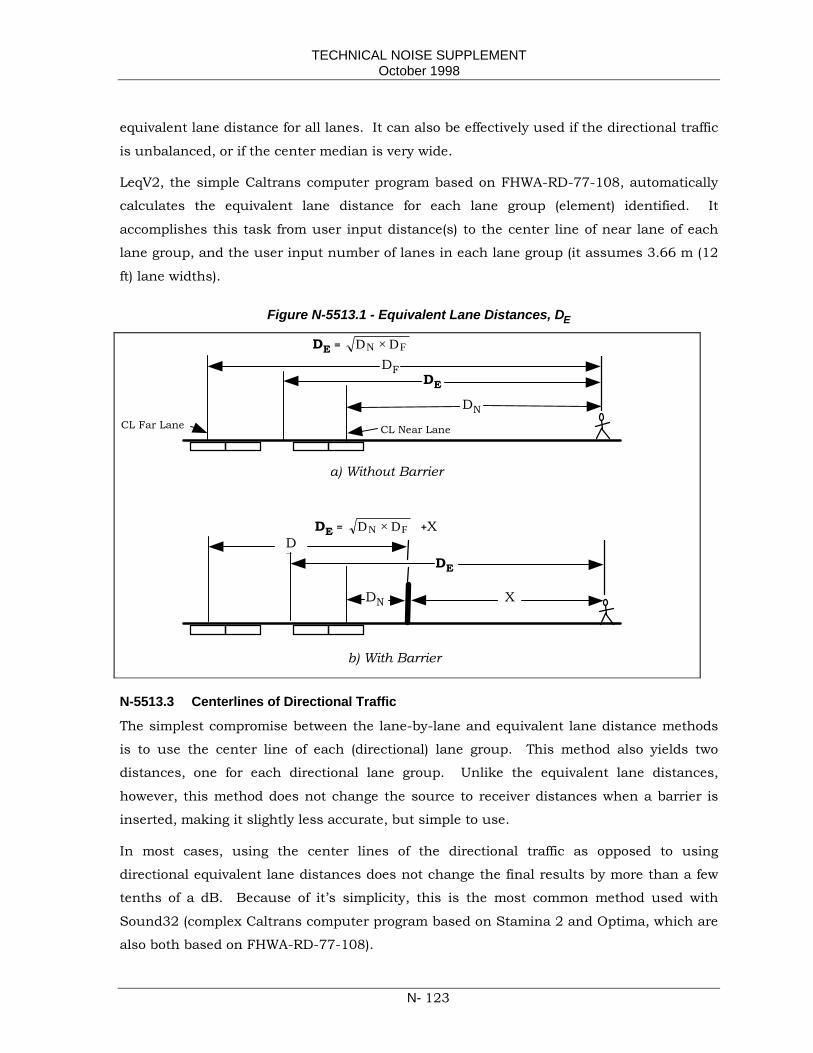
TECHNICAL NOISE SUPPLEMENTOctober 1998
N- 123
equivalent lane distance for all lanes. It can also be effectively used if the directional traffic
is unbalanced, or if the center median is very wide.
LeqV2, the simple Caltrans computer program based on FHWA-RD-77-108, automatically
calculates the equivalent lane distance for each lane group (element) identified. It
accomplishes this task from user input distance(s) to the center line of near lane of each
lane group, and the user input number of lanes in each lane group (it assumes 3.66 m (12
ft) lane widths).
Figure N-5513.1 - Equivalent Lane Distances, DE
N-5513.3 Centerlines of Directional Traffic
The simplest compromise between the lane-by-lane and equivalent lane distance methods
is to use the center line of each (directional) lane group. This method also yields two
distances, one for each directional lane group. Unlike the equivalent lane distances,
however, this method does not change the source to receiver distances when a barrier is
inserted, making it slightly less accurate, but simple to use.
In most cases, using the center lines of the directional traffic as opposed to using
directional equivalent lane distances does not change the final results by more than a few
tenths of a dB. Because of it’s simplicity, this is the most common method used with
Sound32 (complex Caltrans computer program based on Stamina 2 and Optima, which are
also both based on FHWA-RD-77-108).
DN
DE
DF
a) Without Barrier
CL Near LaneCL Far Lane
DE = D DN F×
DN
DE
DF
X
b) With Barrier
DE = D DN F× +X

TECHNICAL NOISE SUPPLEMENTOctober 1998
N- 124
N-5514 Finite Roadway AdjustmentWhen the roadway is not infinitely long in both directions in relationship to the observer, it
becomes necessary to adjust the reference levels to account for only that energy coming
from a portion of the roadway. It is often necessary to separate a roadway into sections to
account for changes in topography, traffic flows, shielding etc.
For hard sites where the drop-off rate is 3 dBA/DD (α= 0) the adjustment is simply:
Finite Roadway Adjustment - Hard Site = 10 Log10
∆φ
180 (eq. N-5514-1)
Where:
∆φ = φ1 − φ2
φ1 and φ2 are angles in degrees as shown in Figure N-5514-1.
Note that in all cases ∆φ will be positive and will be numerically equal to the included angle
subtended by the roadway relative to the receiver.
For soft sites, where the drop-off rate is 4.5 dBA/DD (α = 0.5), the adjustment is more
complex since the excess distance attenuation must also be accounted for:
Finite Roadway Adjustment - Soft Site = 10 Log10 1π φ1
∫φ2
cosφ dφ (eq. N-5514-2)
N-5515 Shielding Adjustments
Shielding is one of the most effective ways of reducing traffic noise. Shielding occurs when
the observer's view of the highway is obstructed or partially obstructed by natural or man-
made features interfering with the propagation of the sound waves. Figure N-5515.1
illustrates the general rules of thumb for various shielding adjustments.
Figure N-5515.1 shows the attenuation credit given by the FHWA model to plantings,
woods and vegetation: 5 dBA for the first 30 m (100 ft), with an additional 5 dBA for the
second 30 m. The height of the trees should extend at least 5 m (16 ft) above the line of
sight, and the woods must be dense enough to completely block the view of the traffic from
the receiver. Obviously, to be effective throughout the year the trees must be mostly
evergreens. Ordinary landscaping along the highway is not effective in actually reducing
traffic noise, although it may provide a psychological “out of sight, out of mind” effect that
tends to reduce the awareness of traffic noise.

TECHNICAL NOISE SUPPLEMENTOctober 1998
N- 125
Figure N-5514.1 - Identification of Angles
Based on this procedure, only three cases are possible:Case A – Ø 1 is negative, Ø 2 is positive.Case B – Ø 1 is negative, Ø 2 is negative.Case C – Ø 1 is positive, Ø 2 is positive.
Ø 1 Ø 2
A BRoadway Segment
Observer(1) Case A
+90°-90°
0 °
Ø 1 Ø 2
A BRoadway Segment
Observer+90°-90°
0°
(2 ) Case B
Ø 1 Ø 2
AB Roadway Segment
Observer+90° -90°
0°
(3) Case C
The amount of attenuation provided by rows of buildings (d) depends on the size of the gaps
between the buildings. 3 dBA attenuation is allowed for the first row of buildings when
they occupy 40 to 65% of the row (35 to 60% gaps). 5 dBA is allowed when the buildings
occupy 65 to 90% of the row (10 to 35% gaps). Rows of buildings behind the first row are
given 1.5 dBA attenuation each.
While attenuation due to temperature gradients, winds and atmospheric absorption also
occur, they are not accounted for in the FHWA model. Since they may vary by time and
location, their effects are not considered permanent, although these factors become very
important when making measurements. Also, the noise abatement criteria to which the
modeled results are compared are set for normal conditions.

TECHNICAL NOISE SUPPLEMENTOctober 1998
N- 126
Figure N-5515.1 - Shielding Adjustments
3dBA for 40-65% Area 5dBA for 65-90% Area 1.5dBA for Each Additional Row 10dBA max.
SITUATION ATTENUATION
3dBA/DD
4.5dBA/DD
5dBA for 1st 30 m 5dBA for 2nd 30m 10dBA max.
1st ROW
WALL 20dBA max. BERM 23 dBA max.
DD = Doubling Distance
N-5515.1 Noise Barriers
Section N-2144 discussed the general characteristics of noise barriers and principles of
diffraction, transmission loss and barrier atttenuation. Noise barriers can be constructed
of any number of materials. The FHWA model works with the assumptions that:
1. The noise transmitted through the barrier will not contribute to the diffracted noise,i.e. is at least 10 dBA less than the noise diffracted over the top of the barrier. Forthis to be true the barriers transmission loss must be at least 10 dBA greater thanthe noise attenuation due to diffraction. For example, if the desired barrierattenuation is 10 dBA, the transmission loss of the barrier material must be at least20 dBA. See Figure N-5515.2 for the effects of insufficient transmission loss)
2. The barrier cannot have cracks that would allow noise leakage. The FHWA modeldoes not consider any noise that passes through a barrier or that may be diffractedaround the ends of a barrier. (See Section N-6230 for a discussion of the effects ofbarrier openings for maintenance purposes on barrier performance.)
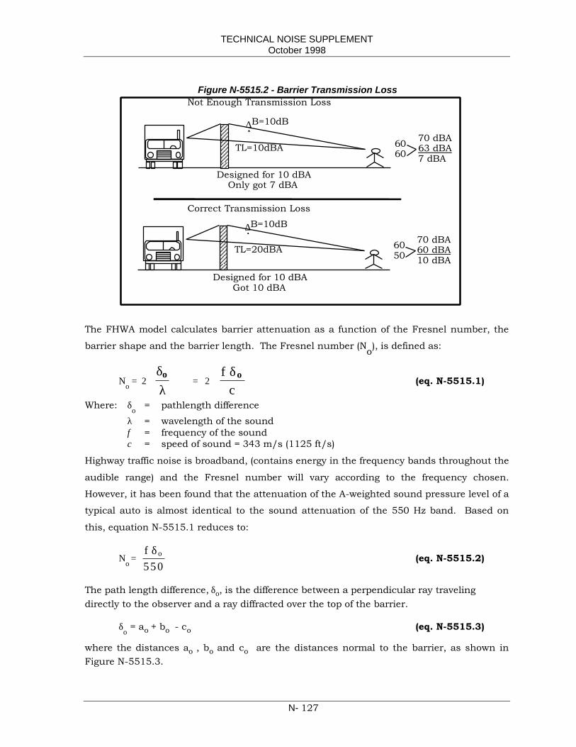
TECHNICAL NOISE SUPPLEMENTOctober 1998
N- 127
Figure N-5515.2 - Barrier Transmission Loss
TL=10dBA
∆B=10dBA
Designed for 10 dBAOnly got 7 dBA
6060
70 dBA63 dBA7 dBA
Not Enough Transmission Loss
TL=20dBA
∆B=10dBA
Designed for 10 dBAGot 10 dBA
6050
70 dBA60 dBA10 dBA
Correct Transmission Loss
The FHWA model calculates barrier attenuation as a function of the Fresnel number, the
barrier shape and the barrier length. The Fresnel number (No), is defined as:
No = 2 δλo
= 2
fc
oδ
(eq. N-5515.1)
Where: δo = pathlength difference
λ = wavelength of the soundf = frequency of the soundc = speed of sound = 343 m/s (1125 ft/s)
Highway traffic noise is broadband, (contains energy in the frequency bands throughout the
audible range) and the Fresnel number will vary according to the frequency chosen.
However, it has been found that the attenuation of the A-weighted sound pressure level of a
typical auto is almost identical to the sound attenuation of the 550 Hz band. Based on
this, equation N-5515.1 reduces to:
No = f 550
oδ(eq. N-5515.2)
The path length difference, δo, is the difference between a perpendicular ray travelingdirectly to the observer and a ray diffracted over the top of the barrier.
δo = ao + bo - co (eq. N-5515.3)
where the distances ao , bo and co
are the distances normal to the barrier, as shown inFigure N-5515.3.

TECHNICAL NOISE SUPPLEMENTOctober 1998
N- 128
Figure N-5515.3 - Path Length Difference and Fresnel Number
For barrier calculation purposes, the vehicle noise sources are also simplified to those
shown in Figure N-5515.4. These heights attempt to take into account and centralize the
locations of the many individual sources of noise radiated from the vehicle types.
ao bo
co
Source
Receiver
“Illuminated” Zone
Shadow Zone
Fresnel Number = 2(Path length Difference / Wave Length)
Path Length Difference = ao + bo - co
ao
bo
co
a
b
c
Source positionyielding max. pathlength difference(normal to barrier)
δ = Path length diff. = a+b-cδo = Max. path length diff. = ao+bo-co
(90o to wall)(skew)
Source positionyielding less thanmax. path lengthdifference (skewedto barrier)

TECHNICAL NOISE SUPPLEMENTOctober 1998
N- 129
Figure N-5515.4 - Vehicle Source Heights Above Pavement
For barriers of finite length, the attenuation provided by a barrier depends on how much of
the roadway is shielded from the observer. As with the finite roadway adjustment for soft
sites, the finite barrier attenuation, ∆Bi, calculations involves the solution of an integral:
∆Bi = 10log10 ( )∫−
R
L
dxLR
φ
φ
φφφ
1, where: (eq. N-5515.4)
X = 1 for Ni < -0.1916 - 0.0635 (eq. N-5515.5)
X = 10 2
10 2
0 3 20
0
−
⋅
. t an coscos
ε ππ φ
φNN
i for (-0.916-0.0635ε)<Ni<0 (eq. N-5515.6)
x = 10 2
10 2
0 3 20
0
−
⋅
. t a n h ( ) cos( ) cos
ε ππ
φφ
NN
i
i for 0<Ni<5.03 Note: tanh(x) = (ex-e-x)/(ex+e-x)
(eq. N-5515.7)
x = 10
10
0 3
0
− . ε for Ni>5.03 (eq. N-5515.8)
Note the ε (epsilon) term in the equations: ε = 0 for a wall, and ε = 3 for a berm. The FHWA
model assumes that earth berms perform about 3 dB better than free standing walls due to
the top of barrier shape. ε accounts for this difference.
ACTUAL HEIGHT
Tires 0 m
Engine 1.5 m (5 ft)Tires 0 m
Exhaust 3.5 m (11.5 ft)Engine 1.5 m (5 ft)Tires 0 m
MODELED HEIGHT
0 m
0.7 m (2.3 ft)
2.4 m (8 ft)
Autos
Medium Trucks
Heavy Trucks

TECHNICAL NOISE SUPPLEMENTOctober 1998
N- 130
N-5515.2 Ground Effects
Consider the situation where the ground between the roadway and the observer is reflective
(the drop-off rate is 3, or α = 0). This situation is illustrated in Figure N-5515.5(a). As was
indicated in Table N-5513.1, under these circumstances the drop-off rate is 3 dBA/DD
[from 3(a)]. When a barrier is constructed between the roadway and the observer, the top of
the barrier appears to be the noise source to the observer and again, the drop-off rate
should be 3 dBA/DD (Figure N-5515.5(b)).
Figure N-5515.5 - Ground Effects
However, when the ground between the roadway and the observer is soft (4.5 dBA/DD, α =0.5) the ground effects can provide an additional 1.5 dBA/DD when both the source and
the receiver are close to the ground (Figure N-5515.5(c)). In this case, when a barrier is
constructed between the observer and the roadway, the top of the barrier again appears to
be the noise source to the observer and the appropriate drop-off rate is 3 dBA/DD (Figure
5515.5(d)). Thus, the 1.5 dBA/DD excess attenuation from the ground effects has been
lost. Constructing a barrier effectively raises the source height and the ground effect is
lost. Consequently, if the barrier attenuation was 9 dBA, an observer at 200 ft would get a
HT.*
MT * A *
*
**
*
**
*
**
a) α = 0
b) α = 0
c) α = 0.5
d) α = 0
Effects of Noise Barrier on α = 0 (a and b) and α = 0.5 (c and d).
TECHNICAL NOISE SUPPLEMENTOctober 1998
N- 131
field insertion loss of only 6 dBA (9 dBA barrier attenuation minus the 3 dBA lost excess
ground effects).
N-5520 FHWA-TRAFFIC NOISE MODEL (FHWA-PD-96-009 &-010; DOT-VNTSC-FHWA-98-1 & -2) OVERVIEW
The FHWA Traffic Noise Model (TNM) was released on March 30, 1998. TNM will replace
the FHWA-RD-77-108 methodology and the computer versions LEQV2 and SOUND32. The
phase in period will be two years from the above date. The model is described in the
“FHWA Traffic Noise Model - Technical Manual “, Report Number: FHWA-PD-96-010;
DOT-VNTSC-FHWA-98-2. The instructions for using the TNM version 1.0 software are
contained in “FHWA Traffic Noise Model - User’s Guide“, Report Number: FHWA-PD-96-
009; DOT-VNTSC-FHWA-98-1.
FHWA TNM is a registered Copyright. The Copyright encompasses the User’s Guide,
Technical Manual, and software source and executable codes. FHWA TNM is also a
registered Trademark. The Trademark encompasses the copyrighted User’s Guide,
Technical Manual, and software source and executable codes. It provides the FHWA with
the exclusive right to use the names “Federal Highway Administration Traffic Noise Model”
and “FHWA TNM”. A TNM package, including the model software, the User’s Guide, the
Technical Manual and a TNM tutorial CD-ROM has been distributed to each Caltrans
District, and Caltrans may make sufficient copies for internal use. All other users must
purchase the TNM package through:
The McTrans Center at the University of Florida, Telephone (904) 392-3225,
Fax: (904) 392-3224, World Wide Web: http://www-mctrans.ce.ufl.edu
Following sections provide a brief overview of TNM. For detailed information the above
referenced TNM Technical Manual and User’s Guide should be consulted.
Limited TNM test runs results have generally agreed within two decibels with Sound 32
results.
N-5521 TNM Reference Energy Mean Emission Levels (REMELs)TNM computes highway traffic noise at nearby receivers and aids in the design of noise
barriers. The noise sources include an entirely new data base of 1994-1995 noise reference
energy mean emission levels (REMELs) that is detailed in “Development of National
Reference Energy Mean Emission Levels for the FHWA Traffic Noise Model (FHWA TNM ),
Version 1.0”, Report Number: FHWA-PD-008; DOT-VNTSC-FHWA-96-2. The database

TECHNICAL NOISE SUPPLEMENTOctober 1998
N- 132
includes speed-dependent emission levels for constant speeds on level roadways from idle
to 80 mph (129 km/h), for the following vehicle types:
• Automobiles: same definition as in FHWA-RD-77-108• Medium Trucks: same definition as in FHWA-RD-77-108• Heavy Trucks: same definition as in FHWA-RD-77-108• Buses: all vehicles designed more than nine passengers; and• Motorcycles: all vehicles with two or three tires and an open-air driver/passenger
compartment
In addition, the database includes data for:
• vehicles on grades• three different pavements (dense-graded asphaltic concrete, open-graded asphaltic
concrete, and Portland cement concrete)• accelerating vehicles• acoustic energy apportioned to two sub-source heights above the pavement: 0 m and
1.5 m (5 ft) for all vehicles, except for heavy trucks where the sub-source heights are 0m and 3.66 m (12 ft)
• data stored in 1/3 octave bands
Figure N-5520.1 compares the new TNM Baseline REMELs with the Calveno REMELs. The
latter were used in SOUND32 and LEQV2 programs (see Section N-5510) and must not be
used with TNM. The TNM Baseline REMEL curves in Figure N-5520.1 were plotted from
the TNM Baseline equations:
Speed 0 km/h (IDLE):L(si) = 10 log10 (10C/10) = (eq.N-5520.1)L(si) = C (eq.N-5520.1a)
Speed > 0 km/h: L(si) = 10 log10 [(0.6214 si)A/10 10B/10 + 10C/10] (eq.N-5520.2)
Where: L(si) = REMEL for vehicle type i, at speed s (km/h)
si = Speed of vehicle type i in km/hA, B, C are constants for each vehicle type, shown below (Table N-5521.1)
Note: For speeds in mph omit 0.6214 in above eq. 2.
Table N-5521.1Constants
Vehicle Type A B CAutos (A) 41.740807 1.148546 50.128316Medium Trucks (MT) (2-axles, dual wheels) 33.918713 20.591046 68.002978Heavy Trucks (HT) (3-axles) 35.879850 21.019665 74.298135
*Baseline REMELs = Reference Energy Mean Emission Levels for the following conditions:• Average Pavement - Average for all pavements in the study, including Concrete (PCC),
Dense-graded Asphalt (DGAC), and Open-graded Asphalt (OGAC)• Level Roadways - Grades of 1.5 % or less• Constant-Flow Traffic• A-weighted, Total Noise Level at 15 m (50 feet)
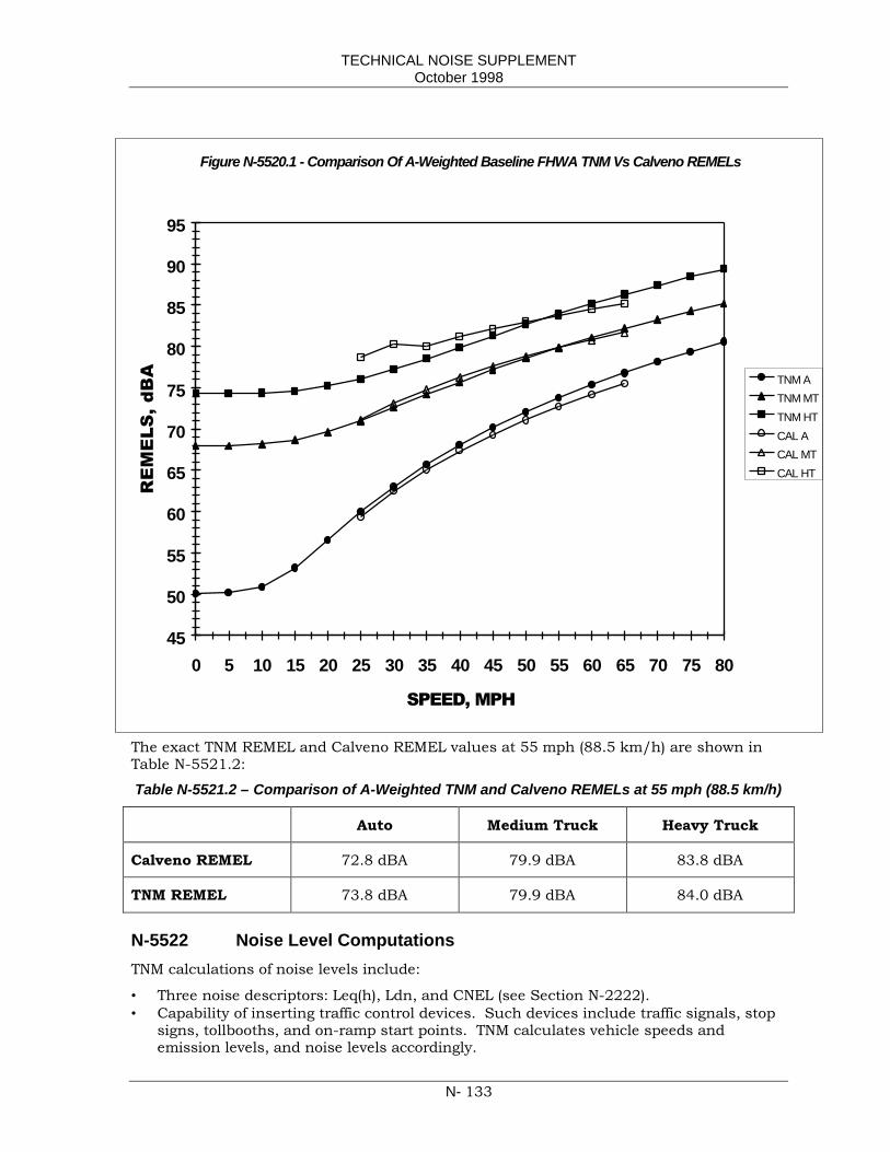
TECHNICAL NOISE SUPPLEMENTOctober 1998
N- 133
The exact TNM REMEL and Calveno REMEL values at 55 mph (88.5 km/h) are shown inTable N-5521.2:
Table N-5521.2 – Comparison of A-Weighted TNM and Calveno REMELs at 55 mph (88.5 km/h)
Auto Medium Truck Heavy Truck
Calveno REMEL 72.8 dBA 79.9 dBA 83.8 dBA
TNM REMEL 73.8 dBA 79.9 dBA 84.0 dBA
N-5522 Noise Level ComputationsTNM calculations of noise levels include:
• Three noise descriptors: Leq(h), Ldn, and CNEL (see Section N-2222).• Capability of inserting traffic control devices. Such devices include traffic signals, stop
signs, tollbooths, and on-ramp start points. TNM calculates vehicle speeds andemission levels, and noise levels accordingly.
Figure N-5520.1 - Comparison Of A-Weighted Baseline FHWA TNM Vs Calveno REMELs
45
50
55
60
65
70
75
80
85
90
95
0 5 10 15 20 25 30 35 40 45 50 55 60 65 70 75 80
SPEED, MPH
REM
ELS,
dBA TNM A
TNM MTTNM HTCAL ACAL MTCAL HT

TECHNICAL NOISE SUPPLEMENTOctober 1998
N- 134
• Computations performed in 1/3 octave bands for greater accuracy (not visible to users).• Noise contours if specified.
Roadways and roadway segments define noise source locations (x-y-z-coordinates). Hourly
traffic volumes determine the noise characteristics of the source.
N-5523 Propagation, Shielding, and Ground EffectsTNM incorporates state-of-the art sound propagation and shielding (e.g. noise barriers)
algorithms, which are based on recent research of sound propagation over different ground
types, atmospheric absorption, and shielding effects of noise barriers (including earth
berms), ground, buildings and trees. However, TNM does not include the effects of
atmospheric refraction, such as varying wind speed and direction or temperature gradients.
TNM propagation algorithms assume neutral atmospheric conditions (zero wind speed,
isothermal atmosphere).
The propagation algorithms can use the following user input information:
• Terrain lines (x-y-z coordinates) define ground location. Height above the ground isimportant in noise propagation.
• Ground zones (x-y-z coordinates) define perimeters of selected ground types. The lattermay be selected from either a ground types menu (e.g., lawn, field grass, pavement,etc.), specified default, or user input flow resistivity (if known).
• Berms may be defined with user-selectable heights, top widths, and side slopes; theyare computed as if they are terrain lines.
• Rows of buildings (x-y-z coordinates) with percentage of area shielded relative to theroadway(s) may be input to calculate additional attenuation.
• Tree zones (x-y-z coordinates) may be included for additional attenuation calculations ifappropriate.
The propagation algorithms also include double diffraction. The net effect from the most
effective pair of barriers, berms, or ground points that intercept the source-receiver line of
sight is computed.
N-5524 Parallel Barrier Analysis
TNM includes a multiple reflection module that computes a degradation of the performance
of one reflective barrier in the presence of another reflective barrier on the opposite side of
the roadway. Unlike other TNM acoustics, which are computed in three dimensions, the
multiple reflection module computes the results from a two dimensional cross-section. The
results of this module are used to modify the TNM noise levels.
N-5600 COMPARING RESULTS WITH APPROPRIATECRITERIA
After the predicted noise levels (including model calibration, if appropriate) have been
determined they should be compared with the appropriate impact criteria in the Traffic

TECHNICAL NOISE SUPPLEMENTOctober 1998
N- 135
Noise Analysis Protocol, Section 2.4. Examination of traffic noise impacts includes
comparing for each project alternative the following:
a) Predicted noise levels with existing noise levels (Section 2.4.1)b) Predicted noise levels with the appropriate Noise Abatement Criterion (Section 2.4.2)c) Predicted noise level of classroom interior with 52 dBA Leq(h) (Section 2.5)
N-5700 EVALUATING NOISE ABATEMENT OPTIONSIf traffic noise impacts have been identified, noise abatement must be considered as
discussed in the Traffic Noise Analysis Protocol, Sections 2.7 (Noise Abatement Feasibility)
and 2.8 (Noise Abatement Reasonableness). Noise abatement measures may include, but
are not necessarily limited to the measures listed in Traffic Noise Analysis Protocol Section
5.3. These potential measures are based on avoiding impacts, interrupting the noise paths,
or protecting selected receivers. If the project alternative locations are flexible, alignments
and profiles can be selected to avoid sensitive receivers or lessen the noise impacts. Most
often highway alignments and profiles are selected on the basis of other overriding factors.
The construction of noise barriers is then usually the most common noise abatement
option available.
The consideration of noise abatement described in the Traffic Noise Analysis Protocol
Sections 2.7 and 2.8 requires at a minimum a preliminary design of the abatement. The
following Section N-6000 gives guidance on the design considerations of noise barriers.

TECHNICAL NOISE SUPPLEMENTOctober 1998
N- 136
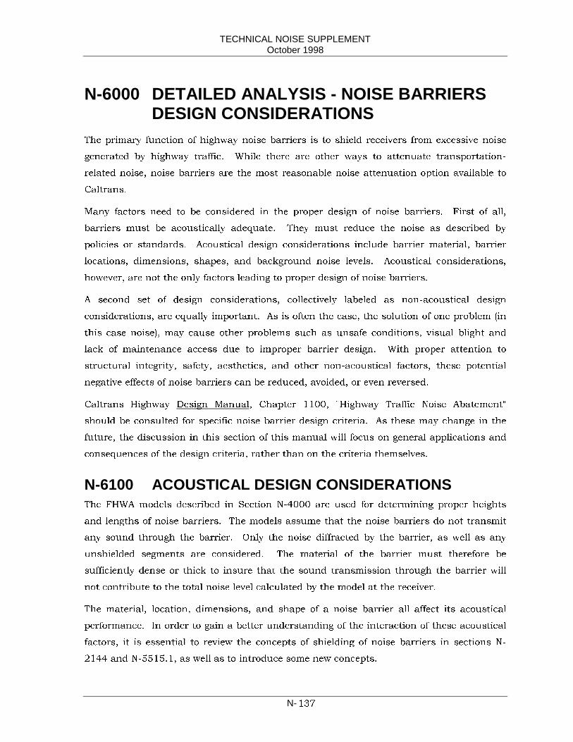
TECHNICAL NOISE SUPPLEMENTOctober 1998
N-���
N-6000 DETAILED ANALYSIS - NOISE BARRIERSDESIGN CONSIDERATIONS
7KH SULPDU\ IXQFWLRQ RI KLJKZD\ QRLVH EDUULHUV LV WR VKLHOG UHFHLYHUV IURP H[FHVVLYH QRLVH
JHQHUDWHG E\ KLJKZD\ WUDIILF� :KLOH WKHUH DUH RWKHU ZD\V WR DWWHQXDWH WUDQVSRUWDWLRQ�
UHODWHG QRLVH� QRLVH EDUULHUV DUH WKH PRVW UHDVRQDEOH QRLVH DWWHQXDWLRQ RSWLRQ DYDLODEOH WR
&DOWUDQV�
0DQ\ IDFWRUV QHHG WR EH FRQVLGHUHG LQ WKH SURSHU GHVLJQ RI QRLVH EDUULHUV� )LUVW RI DOO�
EDUULHUV PXVW EH DFRXVWLFDOO\ DGHTXDWH� 7KH\ PXVW UHGXFH WKH QRLVH DV GHVFULEHG E\
SROLFLHV RU VWDQGDUGV� $FRXVWLFDO GHVLJQ FRQVLGHUDWLRQV LQFOXGH EDUULHU PDWHULDO� EDUULHU
ORFDWLRQV� GLPHQVLRQV� VKDSHV� DQG EDFNJURXQG QRLVH OHYHOV� $FRXVWLFDO FRQVLGHUDWLRQV�
KRZHYHU� DUH QRW WKH RQO\ IDFWRUV OHDGLQJ WR SURSHU GHVLJQ RI QRLVH EDUULHUV�
$ VHFRQG VHW RI GHVLJQ FRQVLGHUDWLRQV� FROOHFWLYHO\ ODEHOHG DV QRQ�DFRXVWLFDO GHVLJQ
FRQVLGHUDWLRQV� DUH HTXDOO\ LPSRUWDQW� $V LV RIWHQ WKH FDVH� WKH VROXWLRQ RI RQH SUREOHP �LQ
WKLV FDVH QRLVH�� PD\ FDXVH RWKHU SUREOHPV VXFK DV XQVDIH FRQGLWLRQV� YLVXDO EOLJKW DQG
ODFN RI PDLQWHQDQFH DFFHVV GXH WR LPSURSHU EDUULHU GHVLJQ� :LWK SURSHU DWWHQWLRQ WR
VWUXFWXUDO LQWHJULW\� VDIHW\� DHVWKHWLFV� DQG RWKHU QRQ�DFRXVWLFDO IDFWRUV� WKHVH SRWHQWLDO
QHJDWLYH HIIHFWV RI QRLVH EDUULHUV FDQ EH UHGXFHG� DYRLGHG� RU HYHQ UHYHUVHG�
&DOWUDQV +LJKZD\ 'HVLJQ 0DQXDO� &KDSWHU ����� �+LJKZD\ 7UDIILF 1RLVH $EDWHPHQW�
VKRXOG EH FRQVXOWHG IRU VSHFLILF QRLVH EDUULHU GHVLJQ FULWHULD� $V WKHVH PD\ FKDQJH LQ WKH
IXWXUH� WKH GLVFXVVLRQ LQ WKLV VHFWLRQ RI WKLV PDQXDO ZLOO IRFXV RQ JHQHUDO DSSOLFDWLRQV DQG
FRQVHTXHQFHV RI WKH GHVLJQ FULWHULD� UDWKHU WKDQ RQ WKH FULWHULD WKHPVHOYHV�
N-6100 ACOUSTICAL DESIGN CONSIDERATIONS7KH )+:$ PRGHOV GHVFULEHG LQ 6HFWLRQ 1����� DUH XVHG IRU GHWHUPLQLQJ SURSHU KHLJKWV
DQG OHQJWKV RI QRLVH EDUULHUV� 7KH PRGHOV DVVXPH WKDW WKH QRLVH EDUULHUV GR QRW WUDQVPLW
DQ\ VRXQG WKURXJK WKH EDUULHU� 2QO\ WKH QRLVH GLIIUDFWHG E\ WKH EDUULHU� DV ZHOO DV DQ\
XQVKLHOGHG VHJPHQWV DUH FRQVLGHUHG� 7KH PDWHULDO RI WKH EDUULHU PXVW WKHUHIRUH EH
VXIILFLHQWO\ GHQVH RU WKLFN WR LQVXUH WKDW WKH VRXQG WUDQVPLVVLRQ WKURXJK WKH EDUULHU ZLOO
QRW FRQWULEXWH WR WKH WRWDO QRLVH OHYHO FDOFXODWHG E\ WKH PRGHO DW WKH UHFHLYHU�
7KH PDWHULDO� ORFDWLRQ� GLPHQVLRQV� DQG VKDSH RI D QRLVH EDUULHU DOO DIIHFW LWV DFRXVWLFDO
SHUIRUPDQFH� ,Q RUGHU WR JDLQ D EHWWHU XQGHUVWDQGLQJ RI WKH LQWHUDFWLRQ RI WKHVH DFRXVWLFDO
IDFWRUV� LW LV HVVHQWLDO WR UHYLHZ WKH FRQFHSWV RI VKLHOGLQJ RI QRLVH EDUULHUV LQ VHFWLRQV 1�
���� DQG 1�������� DV ZHOO DV WR LQWURGXFH VRPH QHZ FRQFHSWV�

TECHNICAL NOISE SUPPLEMENTOctober 1998
N-���
)LJXUH 1������� LV D VLPSOLILHG VNHWFK VKRZLQJ ZKDW KDSSHQV WR YHKLFOH QRLVH ZKHQ D QRLVH
EDUULHU �VRXQG ZDOO� LV SODFHG EHWZHHQ WKH VRXUFH �YHKLFOH� DQG UHFHLYHU� 7KH RULJLQDO
VWUDLJKW OLQH SDWK IURP WKH VRXUFH WR WKH UHFHLYHU LV QRZ LQWHUUXSWHG E\ WKH EDUULHU�
'HSHQGLQJ RQ WKH EDUULHU PDWHULDO DQG VXUIDFH WUHDWPHQW� D SRUWLRQ RI WKH RULJLQDO QRLVH
HQHUJ\ LV UHIOHFWHG RU VFDWWHUHG EDFN WRZDUGV WKH VRXUFH� $QRWKHU SRUWLRQ LV DEVRUEHG E\
WKH PDWHULDO RI WKH EDUULHU� ZKLOH VWLOO DQRWKHU SRUWLRQ LV WUDQVPLWWHG WKURXJK WKH EDUULHU�
1RWLFH WKDW WKH UHIOHFWHG �VFDWWHUHG� DQG DEVRUEHG QRLVH SDWKV QHYHU UHDFK WKH UHFHLYHU�
Figure N-6100.1 Alteration of Noise Paths by a Noise Barrier
7KH WUDQVPLWWHG QRLVH� KRZHYHU� FRQWLQXHV RQ WR WKH UHFHLYHU ZLWK D ´ORVVµ RI DFRXVWLFDO
HQHUJ\ �DFRXVWLFDO HQHUJ\ UHGLUHFWHG DQG VRPH FRQYHUWHG LQWR KHDW�� 7KH FRPPRQ ORJDULWKP
RI HQHUJ\ UDWLRV RI WKH QRLVH LQ IURQW RI WKH EDUULHU DQG EHKLQG WKH EDUULHU� H[SUHVVHG LQ
GHFLEHOV� LV FDOOHG WKH WUDQVPLVVLRQ ORVV �7/�� 7KH 7/ RI D EDUULHU GHSHQGV RQ WKH EDUULHU
PDWHULDO �PDLQO\ LWV ZHLJKW�� DQG WKH IUHTXHQF\ VSHFWUXP RI WKH QRLVH VRXUFH�
7KH WUDQVPLWWHG QRLVH LV QRW WKH RQO\ QRLVH IURP WKH VRXUFH UHDFKLQJ WKH UHFHLYHU� 7KH
VWUDLJKW OLQH QRLVH SDWK IURP WKH VRXUFH WR WKH WRS RI WKH EDUULHU� RULJLQDOO\ GHVWLQHG LQ WKH
GLUHFWLRQ RI $ ZLWKRXW WKH EDUULHU� QRZ LV GLIIUDFWHG GRZQZDUG WRZDUGV WKH UHFHLYHU �)LJXUH
1��������� 7KLV SURFHVV DOVR UHVXOWV LQ D ´ORVVµ RI DFRXVWLFDO HQHUJ\�
7KH UHFHLYHU LV WKXV H[SRVHG WR WKH WUDQVPLWWHG DQG GLIIUDFWHG QRLVH� :KHUHDV WKH
WUDQVPLWWHG QRLVH RQO\ GHSHQGV RQ EDUULHU PDWHULDO SURSHUWLHV� WKH GLIIUDFWHG QRLVH GHSHQGV
RQ WKH ORFDWLRQ� VKDSH� DQG GLPHQVLRQV RI WKH EDUULHU� 7KHVH IDFWRUV ZLOO EH GLVFXVVHG LQ WKH
IROORZLQJ VHFWLRQV�
5HFHLYHU
5HFHLYHU
6RXUFH
1RLVH %DUULHU
7UDQVPLWWHG 3DWK
'LIIUDFWHG 3DWK5HIOHFWHG 3DWK
'LUHFW 3DWK6RXUFH
$
TECHNICAL NOISE SUPPLEMENTOctober 1998
N-���
Figure N-6100.2 Barrier Diffraction
N-6110 Barrier Material, Transmission Loss
)RU DFRXVWLFDO SXUSRVHV� DQ\ PDWHULDO PD\ EH XVHG IRU D EDUULHU EHWZHHQ D QRLVH VRXUFH
DQG D QRLVH UHFHLYHU DV ORQJ DV LW KDV D WUDQVPLVVLRQ ORVV �7/� RI DW OHDVW �� G%$ JUHDWHU
WKDQ WKH GHVLUHG QRLVH UHGXFWLRQ� 7KLV LQVXUHV WKDW WKH RQO\ QRLVH SDWK WR EH FRQVLGHUHG LQ
WKH DFRXVWLFDO GHVLJQ RI D QRLVH EDUULHU LV WKH GLIIUDFWHG QRLVH SDWK�
)RU H[DPSOH� LI D QRLVH EDUULHU LV GHVLJQHG WR UHGXFH WKH QRLVH OHYHO DW D UHFHLYHU E\ � G%$�
WKH 7/ RI WKH EDUULHU PXVW EH DW OHDVW �� G%$� 7KH WUDQVPLWWHG QRLVH PD\ WKHQ EH LJQRUHG�
EHFDXVH WKH GLIIUDFWHG QRLVH LV DW OHDVW �� G%$ JUHDWHU�
$V D UXOH RI WKXPE� DQ\ PDWHULDO ZHLJKLQJ � OEV�VT IW RU PRUH KDV D WUDQVPLVVLRQ ORVV RI DW
OHDVW �� G%$� 6XFK PDWHULDO ZRXOG EH DGHTXDWH IRU D QRLVH UHGXFWLRQ RI DW OHDVW �� G%$
GXH WR GLIIUDFWLRQ� WKLV LV WKH DYHUDJH QRLVH UHGXFWLRQ RI &DOWUDQV QRLVH EDUULHUV� 1RWH WKDW D
ZHLJKW RI � OEV�VT�IW FDQ EH DWWDLQHG E\ OLJKWHU DQG WKLFNHU� RU KHDYLHU DQG WKLQQHU
PDWHULDOV� 7KH JUHDWHU WKH GHQVLW\ RI WKH PDWHULDO� WKH WKLQQHU WKH PDWHULDO PD\ EH� 7/ DOVR
GHSHQGV RQ WKH VWLIIQHVV RI WKH EDUULHU PDWHULDO DQG IUHTXHQF\ RI WKH VRXUFH�
%DUULHU WKHRU\ XVHG LQ WKH )+:$ 0RGHO VWDWHV WKDW WKH PD[LPXP QRLVH UHGXFWLRQ WKDW FDQ
EH DFKLHYHG LV �� G%$ IRU WKLQ VFUHHQV �ZDOOV� DQG �� G%$ IRU EHUPV� $ PDWHULDO WKDW KDV D
7/ RI �� G%$ RU JUHDWHU ZRXOG WKHUHIRUH DOZD\V EH DGHTXDWH IRU D QRLVH EDUULHU LQ DQ\
VLWXDWLRQ�
7DEOH 1������� JLYHV DSSUR[LPDWH 7/ YDOXHV IRU VRPH FRPPRQ PDWHULDOV� WHVWHG IRU W\SLFDO
$�ZHLJKWHG WUDIILF IUHTXHQF\ VSHFWUD� 7KH\ PD\ EH XVHG DV D URXJK JXLGH LQ DFRXVWLFDO
GHVLJQ RI QRLVH EDUULHUV� )RU DFFXUDWH YDOXHV� FRQVXOW PDWHULDO WHVW UHSRUWV E\ DFFUHGLWHG
ODERUDWRULHV� 7KHVH XVXDOO\ DFFRPSDQ\ OLWHUDWXUH SURYLGHG E\ WKH PDQXIDFWXUHU RI WKH
PDWHULDOV�
6RXUFH 5HFHLYHU
'LIIUDFWHG 3DWK
6WUDLJKW 3DWK
6KDGRZ =RQH
$
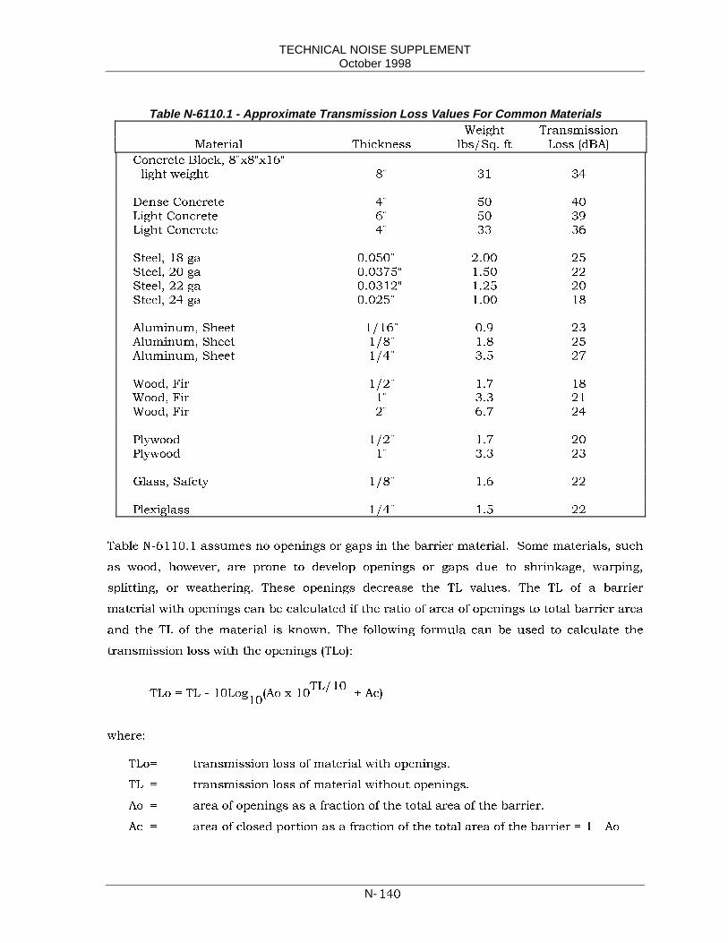
TECHNICAL NOISE SUPPLEMENTOctober 1998
N-���
Table N-6110.1 - Approximate Transmission Loss Values For Common Materials:HLJKW 7UDQVPLVVLRQ
0DWHULDO 7KLFNQHVV OEV�6T� IW /RVV �G%$�
&RQFUHWH %ORFN� ��[��[���
OLJKW ZHLJKW �� �� ��
'HQVH &RQFUHWH �� �� ��
/LJKW &RQFUHWH �� �� ��
/LJKW &RQFUHWH �� �� ��
6WHHO� �� JD ������ ���� ��
6WHHO� �� JD ������� ���� ��
6WHHO� �� JD ������� ���� ��
6WHHO� �� JD ������ ���� ��
$OXPLQXP� 6KHHW ����� ��� ��
$OXPLQXP� 6KHHW ���� ��� ��
$OXPLQXP� 6KHHW ���� ��� ��
:RRG� )LU ���� ��� ��
:RRG� )LU �� ��� ��
:RRG� )LU �� ��� ��
3O\ZRRG ���� ��� ��
3O\ZRRG �� ��� ��
*ODVV� 6DIHW\ ���� ��� ��
3OH[LJODVV ���� ��� ��
7DEOH 1������� DVVXPHV QR RSHQLQJV RU JDSV LQ WKH EDUULHU PDWHULDO� 6RPH PDWHULDOV� VXFK
DV ZRRG� KRZHYHU� DUH SURQH WR GHYHORS RSHQLQJV RU JDSV GXH WR VKULQNDJH� ZDUSLQJ�
VSOLWWLQJ� RU ZHDWKHULQJ� 7KHVH RSHQLQJV GHFUHDVH WKH 7/ YDOXHV� 7KH 7/ RI D EDUULHU
PDWHULDO ZLWK RSHQLQJV FDQ EH FDOFXODWHG LI WKH UDWLR RI DUHD RI RSHQLQJV WR WRWDO EDUULHU DUHD
DQG WKH 7/ RI WKH PDWHULDO LV NQRZQ� 7KH IROORZLQJ IRUPXOD FDQ EH XVHG WR FDOFXODWH WKH
WUDQVPLVVLRQ ORVV ZLWK WKH RSHQLQJV �7/R��
7/R 7/ � ��/RJ��
�$R [ ��7/���
� $F�
ZKHUH�
7/R WUDQVPLVVLRQ ORVV RI PDWHULDO ZLWK RSHQLQJV�
7/ WUDQVPLVVLRQ ORVV RI PDWHULDO ZLWKRXW RSHQLQJV�
$R DUHD RI RSHQLQJV DV D IUDFWLRQ RI WKH WRWDO DUHD RI WKH EDUULHU�
$F DUHD RI FORVHG SRUWLRQ DV D IUDFWLRQ RI WKH WRWDO DUHD RI WKH EDUULHU � � $R

TECHNICAL NOISE SUPPLEMENTOctober 1998
N-���
7KH DERYH PHWKRG RI FDOFXODWLRQ DVVXPHV WKDW WKH RSHQLQJV RU JDSV DUH HTXDOO\ GLVWULEXWHG
RYHU WKH VXUIDFH RI D EDUULHU�
)RU H[DPSOH� D EDUULHU PDGH RI �� WKLFN ILU SODQNV KDV RSHQLQJV WKDW PDNH XS DERXW �� RI
WKH WRWDO DUHD� DQG DUH PRUH RU OHVV HTXDOO\ GLVWULEXWHG� :KDW LV WKH WUDQVPLVVLRQ ORVV RI WKH
PDWHULDO ZLWK WKHVH JDSV"
)URP 7DEOH 1������� LW LV IRXQG WKDW WKH 7/ IRU �� ILU LV �� G%$� 7KH $R LV ��� RU ����� $F
LV ������ �����
7/R �� � ��/RJ��
����� [ �����
� ����� ����� RU DERXW �� G%$
7KH UHGXFHG 7/ FRXOG KDYH DQ HIIHFW RQ WKH EDUULHUV SHUIRUPDQFH� )RU H[DPSOH� DVVXPH
WKDW WKH EHIRUH EDUULHU QRLVH OHYHO ZDV �� G%$ DQG WKH LQWHQWLRQ ZDV WR UHGXFH QRLVH OHYHOV
E\ �� G%$ �L�H�� WKH GLIIUDFWHG QRLVH ZDV WR EH �� G%$ DQG WKH WUDQVPLWWHG QRLVH �� � ��
�� G%$�� 7KH WRWDO QRLVH OHYHO ZRXOG KDYH EHHQ �� G%$ � �� G%$ �� G%$� :LWK WKH JDSV�
KRZHYHU� WKH WUDQVPLWWHG QRLVH LV QRZ �� � �� �� G%$� DQG WKH WRWDO QRLVH OHYHO LV �� G%$
� �� G%$ ���� G%$� 7KH HIIHFWLYHQHVV RI WKH EDUULHU LV UHGXFHG E\ DOPRVW � G%$� ,QVWHDG
RI D GHVLJQHG QRLVH UHGXFWLRQ RI �� G%$� DQ DFWXDO QRLVH UHGXFWLRQ RI RQO\ � G%$ ZLOO EH
UHDOL]HG LQ WKLV FDVH�
3URSHUO\ WUHDWHG PDWHULDOV ZLOO UHGXFH RU HOLPLQDWH QRLVH OHDNDJH� )RU H[DPSOH� OXPEHU
VKRXOG EH WUHDWHG ZLWK SUHVHUYDWLYHV WKDW SURYLGH SURSHU SHQHWUDWLRQ DQG GR QRW LQWHUIHUH
ZLWK DQ\ SURWHFWLYH FRDWLQJV �VXFK DV SDLQW� WR EH DSSOLHG ODWHU� 7KH ZRRG VKRXOG DOVR KDYH
D ORZ PRLVWXUH FRQWHQW� UHTXLULQJ NLOQ GU\LQJ DIWHU ZDWHUERUQH SUHVHUYDWLYHV KDYH EHHQ
XVHG� :RRG SODQNV VKRXOG KDYH WRQJXH DQG JURRYHV GHHS HQRXJK WR DOORZ IRU VKULQNDJH
ZLWKRXW JDSV WR PDLQWDLQ D KLJK 7/� 6XFK WRQJXH DQG JURRYLQJ LV XVXDOO\ QRQ�VWDQGDUG�
7KHUH DUH VHYHUDO RWKHU UDWLQJV XVHG WR H[SUHVV WKH DELOLW\ RI PDWHULDOV LQ VSHFLILF
FRQVWUXFWLRQ FRQILJXUDWLRQV WR UHVLVW VRXQG WUDQVPLVVLRQ� 7ZR RI WKHVH DUH ZRUWK
PHQWLRQLQJ� 7KH\ DUH WKH 6RXQG 7UDQVPLVVLRQ &ODVV �67&�� DQG WKH ([WHULRU :DOO 1RLVH
5DWLQJ �(:15�� %RWK DUH PRVW RIWHQ XVHG LQ FRQMXQFWLRQ ZLWK LQGRRU DFRXVWLFV�
67& LV XQLYHUVDOO\ DFFHSWHG E\ DUFKLWHFWV DQG HQJLQHHUV� 7KH 67& UDWLQJ XVHV D VWDQGDUG
FRQWRXU DJDLQVW ZKLFK WKH 7/ YDOXHV LQ RQH�WKLUG RFWDYH EDQGV DUH FRPSDUHG LQ WKH
IUHTXHQF\ UDQJH EHWZHHQ ��� +] DQG ���� +]� 7KH VWDQGDUG FRQWRXU LV PRYHG XS RU GRZQ
UHODWLYH WR WKH WHVW FXUYH XQWLO WKH VXP RI WKH GLIIHUHQFHV EHWZHHQ WKHP LV �� G% RU OHVV� DQG
WKH PD[LPXP GLIIHUHQFH DW HDFK ��� RFWDYH FHQWHU IUHTXHQF\ LV QR JUHDWHU WKDQ � G%� 7KH
67& LV WKHQ WKH 7/ YDOXH RI WKH VWDQGDUG FRQWRXU DW WKH ��� +] FHQWHU IUHTXHQF\�

TECHNICAL NOISE SUPPLEMENTOctober 1998
N-���
7KH GLVDGYDQWDJH RI WKH 67& UDWLQJ VFKHPH LV WKDW LW LV GHVLJQHG WR UDWH QRLVH UHGXFWLRQV LQ
IUHTXHQFLHV RI QRUPDO RIILFH DQG VSHHFK QRLVHV� DQG QRW IRU WKH ORZHU IUHTXHQFLHV RI
KLJKZD\ WUDIILF QRLVH� 7KH 67&� KRZHYHU� FDQ VWLOO EH XVHG DV D URXJK JXLGH� EXW LW VKRXOG
EH SRLQWHG RXW WKDW IRU IUHTXHQFLHV RI DYHUDJH WUDIILF FRQGLWLRQV� WKH 67& LV � WR �� G%$
JUHDWHU WKDQ WKH 7/� )RU H[DPSOH� PDWHULDO ZLWK DQ 67& UDWLQJ RI �� KDV D 7/ RI DERXW �� �
�� G%$ IRU WUDIILF QRLVH�
7KH (:15 UDWLQJ VFKHPH LV GLIIHUHQW IURP WKH 67&� LQ WKDW LW XVHV D VWDQGDUG FRQWRXU
GHYHORSHG IURP WUDQVSRUWDWLRQ QRLVH IUHTXHQFLHV� ,W WKHUHIRUH DJUHHV FORVHO\ ZLWK WKH $�
ZHLJKWHG 7/ IRU WUDIILF QRLVH�
7KH )HGHUDO +LJKZD\ $GPLQLVWUDWLRQ UHSRUW� ,QVXODWLRQ RI %XLOGLQJV $JDLQVW +LJKZD\ 1RLVH�
)+:$�76������� SURYLGHV IXUWKHU XVHIXO LQIRUPDWLRQ IRU FDOFXODWLQJ RXWGRRU WR LQGRRU
WUDIILF QRLVH UHGXFWLRQV�
N-6120 Barrier Location
7KH SUHYLRXV VHFWLRQ LQGLFDWHG WKDW E\ VHOHFWLQJ PDWHULDOV ZLWK VXIILFLHQW 7/� QRLVH
WUDQVPLWWHG WKURXJK D EDUULHU PD\ EH LJQRUHG VLQFH LWV FRQWULEXWLRQ WR WKH WRWDO QRLVH OHYHO
LV QHJOLJLEOH �OHVV WKDQ ��� G%$��
7KH RQO\ UHPDLQLQJ QRLVH RI FRQFHUQ WKHQ� LV WKH GLIIUDFWHG QRLVH� 6HFWLRQV 1����� DQG 1�
������ GLVFXVVHG WKH EDVLFV RI GLIIUDFWLRQ DQG EDUULHU DWWHQXDWLRQ� 7KH SULQFLSDO IDFWRU
GHWHUPLQLQJ EDUULHU DWWHQXDWLRQ LV WKH )UHVQHO 1XPEHU� ZKLFK LV UHODWHG WR WKH SDWK OHQJWK
GLIIHUHQFH �3/'� EHWZHHQ WKH RULJLQDO� VWUDLJKW OLQH SDWK EHWZHHQ VRXUFH DQG UHFHLYHU� DQG
WKH GLIIUDFWHG SDWK� GHVFULEHG E\ VRXUFH�WRS RI EDUULHU�UHFHLYHU� 7KH JUHDWHU WKLV GLIIHUHQFH�
WKH JUHDWHU WKH EDUULHU DWWHQXDWLRQ �XS WR D OLPLW RI �� G% IRU ZDOOV� DQG �� G% IRU EHUPV��
)LJXUH 1������� VKRZV WKH 3/' FRQFHSW�
Figure N-6120.1 - Path Length Difference
8
✳
DE
F
7RS RI%DUULHU
3DWK /HQJWK 'LIIHUHQFH �3/'� D � E � F
6RXUFH
5HFHLYHU

TECHNICAL NOISE SUPPLEMENTOctober 1998
N-���
,Q OHYHO� DW�JUDGH URDGZD\�UHFHLYHU FURVV VHFWLRQV� D QRLVH EDUULHU RI D JLYHQ KHLJKW SURYLGHV
JUHDWHU EDUULHU DWWHQXDWLRQ ZKHQ LW LV SODFHG HLWKHU FORVH WR WKH VRXUFH� RU FORVH WR WKH
UHFHLYHU� 7KH OHDVW HIIHFWLYH ORFDWLRQ ZRXOG EH DERXW KDOIZD\ LQ EHWZHHQ WKH VRXUFH DQG
UHFHLYHU� )LJXUH 1�������D�� E�� DQG F� VKRZV WKHVH VLWXDWLRQV IRU WZR VRXUFH KHLJKWV �DXWRV
DQG KHDY\ WUXFNV�� /RFDWLRQ E� JLYHV WKH ORZHVW EDUULHU DWWHQXDWLRQV IRU D JLYHQ EDUULHU
KHLJKW�
Figure N-6120.2 - Barrier Attenuation as a Function of Location (at-grade highway). Barrierattenuation is least when barrier is located half way between source and receiver (b). Best
locations are near the source (a), or receiver (c).
�� P
+7
$XWR
��� P��� P
��� P
5HFHLYHU
��� P
�� P
+7
$XWR
��� P��� P
��� P
5HFHLYHU
���� P ���� P
�� P
+7
$XWR
��� P��� P
��� P
5HFHLYHU
��� P
%$55,(5 $77(18$7,21�+HDY\ 7UXFNV �+7� �� G%$
$XWRV �� G%$
%$55,(5 $77(18$7,21�
+7 � G%$
$XWRV �� G%$
%$55,(5 $77(18$7,21�+7 ���� G%$
$XWRV �� G%$
D�
E�
F�

TECHNICAL NOISE SUPPLEMENTOctober 1998
N-���
,Q GHSUHVVHG KLJKZD\ VHFWLRQV� WKH EDUULHU LV REYLRXVO\ PRVW HIIHFWLYH QHDU WKH UHFHLYHU RQ
WRS RI WKH FXW �)LJXUH 1��������� 1RWH WKDW WKH ZLWKRXW EDUULHU SDWK LV JHQHUDOO\ QRW D
VWUDLJKW SDWK EHWZHHQ VRXUFH DQG UHFHLYHU� 7KH WRS RI FXW LV DOUHDG\ D IDLUO\ HIIHFWLYH QRLVH
EDUULHU� 7KH 3/' LQ WKLV FDVH LV WKH GLIIHUHQFH EHWZHHQ WKH SDWKV GHVFULEHG E\ VRXUFH�WRS RI
EDUULHU� UHFHLYHU� DQG VRXUFH�WRS RI FXW�UHFHLYHU� 7KH EDUULHU DWWHQXDWLRQ LV WKHQ FDOFXODWHG
IURP WKH GLIIHUHQFH LQ EDUULHU DWWHQXDWLRQ SURYLGHG E\ WKH WRS RI FXW DQG WKH WRS RI WKH QRLVH
EDUULHU�
Figure N-6120.3 - Typical Barrier Location Depressed Highways
6RXUFH
7RS RI&XW
5HFHLYHU�6KLHOGHG %HIRUH $IWHU %DUULHU�
%DUULHU�DW 5�:�
6LQFH WKH DWWHQXDWLRQ SHU LQFUHPHQWDO LQFUHDVH LQ EDUULHU KHLJKW GLPLQLVKHV ZLWK WKH
HIIHFWLYH KHLJKW RI D EDUULHU �VHH 6HF� 1������� WKLV GLIIHUHQFH PD\ EH VPDOO� QRLVH EDUULHUV LQ
GHSUHVVHG KLJKZD\ VHFWLRQV DUH JHQHUDOO\ QRW YHU\ HIIHFWLYH LQ UHGXFLQJ QRLVH� 7KLV LV PRVWO\
EHFDXVH WKH FXW VHFWLRQ E\ LWVHOI PD\ DOUHDG\ EH DQ HIIHFWLYH EDUULHU �HDUWK EHUP��
7KH PRVW HIIHFWLYH ORFDWLRQ RI QRLVH EDUULHUV DORQJ KLJKZD\V RQ ILOOV LV RQ WRS RI WKH
HPEDQNPHQW� DV VKRZQ LQ )LJXUH 1�������� $Q\ DWWHPSW WR SODFH WKH EDUULHU FORVHU WR WKH
UHFHLYHUV ZLOO UHVXOW LQ D KLJKHU EDUULHU IRU WKH VDPH RU OHVV DWWHQXDWLRQ� 7KH VDPH KROGV
WUXH IRU HOHYDWHG KLJKZD\V RQ VWUXFWXUHV� 7KH PRVW HIIHFWLYH EDUULHU ORFDWLRQ IURP DQ
DFRXVWLFDO VWDQGSRLQW LV RQ WRS RI WKH VWUXFWXUH�
7KH IRUHJRLQJ GLVFXVVLRQV SRLQW RXW WKDW WKH PRVW DFRXVWLFDOO\ HIIHFWLYH ORFDWLRQ IRU D QRLVH
EDUULHU GHSHQGV RQ WKH VRXUFH WR UHFHLYHU JHRPHWU\� ,Q PRVW FDVHV� WKH FKRLFHV DUH IDLUO\
REYLRXV� 7R UHFDS WKH VLPSOHVW VLWXDWLRQV�
�� +LJKZD\ DW�JUDGH� EDUULHU ORFDWLRQ QHDU WKH HGJH RI VKRXOGHU� RU DW WKH ULJKW�RI�ZD\
�5�:��
�� +LJKZD\ LQ GHSUHVVHG VHFWLRQ� EDUULHU DW WKH 5�:�
�� (OHYDWHG KLJKZD\ RQ HPEDQNPHQW RU VWUXFWXUH� EDUULHU QHDU HGJH RI VKRXOGHU�

TECHNICAL NOISE SUPPLEMENTOctober 1998
N-���
Figure N-6120.4 - Typical Barrier Location - Elevated Highways
6RXUFH
5HFHLYHU ��6KLHOGHG %HIRUH $IWHU %DUULHU�
%DUULHU�DW 7RSRI )LOO�
5HFHLYHU ��8QVKLHOGHG %HIRUH�
6KLHOGHG $IWHU %DUULHU�
,Q VRPH FDVHV� KRZHYHU� WKH FKRLFHV DUH QRW VR VLPSOH� ,Q PRUH FRPSOH[ KLJKZD\�UHFHLYHU
JHRPHWULHV� WKH EHVW ORFDWLRQV IURP DQ DFRXVWLFDO VWDQGSRLQW PD\ QRW EH REYLRXV� 7KH\ PD\
KDYH WR EH GHWHUPLQHG E\ XVLQJ WKH )+:$ +LJKZD\ 7UDIILF 1RLVH 3UHGLFWLRQ 0RGHO� IRU
VHYHUDO EDUULHU ORFDWLRQ DOWHUQDWLYHV�
7UDQVLWLRQV EHWZHHQ FXWV DQG ILOOV� UDPSV� DQG LQWHUFKDQJHV DUH VRPH H[DPSOHV RI FDVHV
QHHGLQJ FDUHIXO FRQVLGHUDWLRQ� )LJXUHV 1������� WKURXJK 1������� VKRZ W\SLFDO QRLVH
EDUULHU ORFDWLRQV LQ VRPH RI WKHVH WUDQVLWLRQDO DUHDV� %DUULHU RYHUODSV DUH RIWHQ QHFHVVDU\
LQ WKHVH FDVHV� DV VKRZQ LQ )LJXUHV 1�������� DQG 1��������
Figure N-6120.5 Barriers for Cut and Fill Transitions
%27� :$//
723 ),// %27� :$// 2* 723 &87
),//&87
)UHHZD\
2* 72( ),//
):< 352),/(
723 :$//
723 :$//
PLAN
PROFILE
ZDOOV

TECHNICAL NOISE SUPPLEMENTOctober 1998
N-���
2QH RI WKH PRUH FRPPRQ UHDVRQV IRU EDUULHU RYHUODSV DUH WR SURYLGH PDLQWHQDQFH DFFHVV WR
WKRVH DUHDV ZLWKLQ WKH 5�: WKDW DUH RQ WKH UHFHLYHU VLGH RI QRLVH EDUULHUV �)LJXUH 1���������
7KLV ZLOO EH GLVFXVVHG LQ JUHDWHU GHWDLO LQ WKH PDLQWHQDQFH FRQVLGHUDWLRQ SRUWLRQ RI WKLV
VHFWLRQ�
Figure N-6120.6 - Barriers for Highway on Fill With Off-Ramp
$
$
%DUULHU
%DUULHU
)UHHZD\
):<
2II5DPS
6HFWLRQ $�$
%DUULHUV
2II5DPS
Figure 6120.7 Barriers for Highway in Cut with Off-Ramp
$
$
%DUULHU
)UHHZD\
):<
2II5DPS
6HFWLRQ $�$
%DUULHU
2II5DPS
7RS RI&XW
5HVWULFWLRQV RQ ODWHUDO FOHDUDQFHV� VLJKW GLVWDQFHV DQG RWKHU VDIHW\ FRQVLGHUDWLRQV PD\ DOVR
GLFWDWH ILQDO QRLVH EDUULHU ORFDWLRQV� 7KH &DOWUDQV +LJKZD\ 'HVLJQ 0DQXDO VKRXOG DOZD\V EH
FRQVXOWHG EHIRUH ILQDOL]LQJ DOWHUQDWH QRLVH EDUULHU DOLJQPHQWV�

TECHNICAL NOISE SUPPLEMENTOctober 1998
N-���
N-6130 Barrier Dimensions (Height and Length)
1RLVH EDUULHU GLPHQVLRQV GHSHQG ODUJHO\ RQ IUHHZD\ JHRPHWU\� WRSRJUDSK\ RI WKH
VXUURXQGLQJ WHUUDLQ� WKH ORFDWLRQ RI WKH QRLVH EDUULHU� DQG WKH VL]H RI WKH DUHD WR EH VKLHOGHG
E\ WKH EDUULHU� $FFRUGLQJ WR VHFWLRQV 1����� DQG 1������ EDUULHU DWWHQXDWLRQ GHSHQGV RQ
WKH SDWK OHQJWK GLIIHUHQFH EHWZHHQ WKH GLUHFW �EHIRUH EDUULHU� DQG GLIIUDFWHG �DIWHU EDUULHU�
QRLVH SDWKV� )LJXUH 1������� UHYLHZHG WKH FRQFHSW� 5HJDUGOHVV RI LWV RULHQWDWLRQ� WKH
WULDQJOH IRUPHG E\ WKH VRXUFH� WRS RI QRLVH EDUULHU DQG WKH UHFHLYHU� ZLOO DOZD\V \LHOG WKH
VDPH EDUULHU DWWHQXDWLRQ� 6LQFH WKH ORFDWLRQ RI WKH ERWWRP RI WKH EDUULHU LV QRW SDUW RI WKH
WULDQJOH� WKH KLJKZD\ JHRPHWU\ DQG WHUUDLQ WRSRJUDSK\ GHWHUPLQH KRZ KLJK WKH EDUULHU
VKRXOG EH IRU D JLYHQ EDUULHU DWWHQXDWLRQ� )LJXUH 1������� VKRZV WKLV FRQFHSW�
6LPLODUO\� WKH OHQJWK RI WKH EDUULHU LV JRYHUQHG E\ WKH H[WHQW RI WKH DUHD WR EH VKLHOGHG DQG
DOVR WKH VLWH JHRPHWU\�WRSRJUDSK\ DV VKRZQ LQ )LJXUH 1��������
Figure N-6130.1 - Actual Noise Barrier Height Depends on Site Geometry and TerrainTopography (same barrier attenuation for a), b), c), and d)).
CROSS SECTIONALVIEW
6RXUFH
7RS %DUULHU
5HFHLYHU
D� E�
F� G�
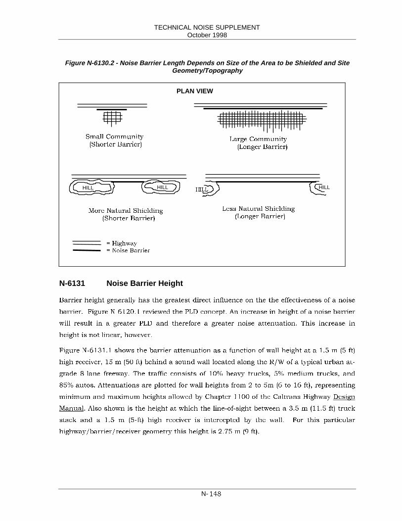
TECHNICAL NOISE SUPPLEMENTOctober 1998
N-���
Figure N-6130.2 - Noise Barrier Length Depends on Size of the Area to be Shielded and SiteGeometry/Topography
N-6131 Noise Barrier Height
%DUULHU KHLJKW JHQHUDOO\ KDV WKH JUHDWHVW GLUHFW LQIOXHQFH RQ WKH WKH HIIHFWLYHQHVV RI D QRLVH
EDUULHU� )LJXUH 1������� UHYLHZHG WKH 3/' FRQFHSW� $Q LQFUHDVH LQ KHLJKW RI D QRLVH EDUULHU
ZLOO UHVXOW LQ D JUHDWHU 3/' DQG WKHUHIRUH D JUHDWHU QRLVH DWWHQXDWLRQ� 7KLV LQFUHDVH LQ
KHLJKW LV QRW OLQHDU� KRZHYHU�
)LJXUH 1������� VKRZV WKH EDUULHU DWWHQXDWLRQ DV D IXQFWLRQ RI ZDOO KHLJKW DW D ��� P �� IW�
KLJK UHFHLYHU� �� P ��� IW� EHKLQG D VRXQG ZDOO ORFDWHG DORQJ WKH 5�: RI D W\SLFDO XUEDQ DW�
JUDGH ��ODQH IUHHZD\� 7KH WUDIILF FRQVLVWV RI ��� KHDY\ WUXFNV� �� PHGLXP WUXFNV� DQG
��� DXWRV� $WWHQXDWLRQV DUH SORWWHG IRU ZDOO KHLJKWV IURP � WR �P �� WR �� IW�� UHSUHVHQWLQJ
PLQLPXP DQG PD[LPXP KHLJKWV DOORZHG E\ &KDSWHU ���� RI WKH &DOWUDQV +LJKZD\ 'HVLJQ
0DQXDO� $OVR VKRZQ LV WKH KHLJKW DW ZKLFK WKH OLQH�RI�VLJKW EHWZHHQ D ��� P ����� IW� WUXFN
VWDFN DQG D ��� P ���IW� KLJK UHFHLYHU LV LQWHUFHSWHG E\ WKH ZDOO� )RU WKLV SDUWLFXODU
KLJKZD\�EDUULHU�UHFHLYHU JHRPHWU\ WKLV KHLJKW LV ���� P �� IW��
HILL HILL +,// HILL
6PDOO &RPPXQLW\
�6KRUWHU %DUULHU�/DUJH &RPPXQLW\
�/RQJHU %DUULHU�
0RUH 1DWXUDO 6KLHOGLQJ
�6KRUWHU %DUULHU�
/HVV 1DWXUDO 6KLHOGLQJ
�/RQJHU %DUULHU�
PLAN VIEW
+LJKZD\
1RLVH %DUULHU

TECHNICAL NOISE SUPPLEMENTOctober 1998
N-���
Figure N-6131.1 Sound Wall Attenuation Vs. Height - At-Grade Freeway
1RWH WKDW LQ WKLV FDVH� WKH FKDQJH LQ DWWHQXDWLRQ SHU LQFUHPHQWDO FKDQJH LQ ZDOO KHLJKW LV
KLJKHVW EHWZHHQ ZDOO KHLJKWV RI ��� DQG ��� P �� � �� IW�� DW ��� G%$ SHU ��� P �� IW�� $ERYH
DQG EHORZ WKLV UDQJH WKH YDOXHV DUH ORZHU� 2QFH WKH RSWLPXP KHLJKW KDV EHHQ UHDFKHG� DQ\
IXUWKHU LQFUHDVHV LQ QRLVH EDUULHU KHLJKW UHVXOW LQ GLPLQLVKLQJ UHWXUQV LQ HIIHFWLYHQHVV�
+RZHYHU� KLJKHU EDUULHUV DUH RIWHQ QHFHVVDU\ WR PHHW GHVLJQ JRDOV�
1RLVH EDUULHUV DORQJ GHSUHVVHG IUHHZD\V DUH OHVV HIIHFWLYH WKDQ WKRVH DORQJ DW�JUDGH
IUHHZD\V� ,Q GHHS FXWV� WKH UHFHLYHU RIWHQ LV DOUHDG\ HIIHFWLYHO\ VKLHOGHG E\ WRSV RI FXWV� ,Q
VRPH FDVHV WKLV VKLHOGLQJ PD\ QRW UHGXFH QRLVH OHYHOV HQRXJK WR VDWLVI\ QRLVH DEDWHPHQW
FULWHULD� DQG DQ DGGLWLRQDO EDUULHU EHKLQG WKH WRS RI FXW PD\ EH QHFHVVDU\ WR DFKLHYH IXUWKHU
QRLVH UHGXFWLRQV�
:KHQ GHVLJQLQJ VXFK D EDUULHU� WKH GHVLJQHU VKRXOG UHFRJQL]H WKDW WKH ZLWKRXW EDUULHU RU
EHIRUH FRQGLWLRQ LQFOXGHV WKH VKLHOGLQJ RI WKH H[LVWLQJ WRS RI FXW� %HFDXVH RI WKH EHIRUH�
PHQWLRQHG GLPLQLVKLQJ UHWXUQV HIIHFW� D EDUULHU RI D JLYHQ KHLJKW DORQJ D GHSUHVVHG IUHHZD\
ZLOO JHQHUDOO\ EH OHVV HIIHFWLYH WKDQ D EDUULHU RI WKH VDPH KHLJKW DW�JUDGH� 7KH GLPLQLVKLQJ
UHWXUQ HIIHFW� KRZHYHU� LV QRW WKH RQO\ WKLQJ WR WDNH LQWR FRQVLGHUDWLRQ�
,W KDV EHHQ PHQWLRQHG WKDW D EHUP LV PRUH HIIHFWLYH WKDQ D ZDOO� &RPSXWHU QRLVH SUHGLFWLRQ
PRGHOV JHQHUDOO\ JLYH EHUPV � G%$ PRUH DWWHQXDWLRQ WKDQ D ZDOO RI WKH VDPH KHLJKW� $ ZDOO
WALL HEIGHT, (m)
1.5 3 4.5 60
0
5
10
15ATTENUATION
(dBA)
• ��/DQH 8UEDQ )UHHZD\� $W�
*UDGH
• 5HFHLYHU �� P %HKLQG WKH
:DOO
• :DOO DW 5�: /LQH
• ��� +HDY\ 7UXFNV
• �� 0HGLXP 7UXFNV
• ��� $XWRV

TECHNICAL NOISE SUPPLEMENTOctober 1998
N-���
EXLOW DW RU QHDU WKH WRS RI FXW HVVHQWLDOO\ HOLPLQDWHV WKH � G%$ H[WUD DWWHQXDWLRQ DIIRUGHG E\
WKH RULJLQDO WRS RI FXW� WKHUHE\ IXUWKHU UHGXFLQJ WKH HIIHFWLYHQHVV RI WKH ZDOO�
)LJXUH 1������� VKRZV WKH EDUULHU DWWHQXDWLRQ YV� KHLJKW SORWV IRU D UHFHLYHU �� P ��� IW�
EHKLQG D EDUULHU ORFDWHG RQ WKH 5�: RI D W\SLFDO XUEDQ ��ODQH IUHHZD\� LQ D ��� P ��� IW�
GHHS GHSUHVVHG VHFWLRQ� 7KH WUDIILF PL[ LV WKH VDPH DV WKDW IRU )LJXUH 1�������� GHVFULEHG
DERYH� 7ZR DWWHQXDWLRQ FXUYHV DUH VKRZQ�
7KH XSSHU FXUYH UHSUHVHQWV DWWHQXDWLRQ GLIIHUHQFHV EHWZHHQ D ZDOO �DIWHU FRQVWUXFWLRQ
FRQGLWLRQ�� DQG WKH WRS RI FXW �EHIRUH FRQVWUXFWLRQ FRQGLWLRQ�� LQ ZKLFK WKH ODWWHU LV WUHDWHG
DV DQ H[LVWLQJ ZDOO� 6XFK D FRQGLWLRQ ZRXOG H[LVW LI D VRXQG ZDOO ZHUH EXLOW RQ WRS RI DQ
H[LVWLQJ UHWDLQLQJ ZDOO� L�H�� WKH WRS RI FXW ZRXOG EH WKH WRS RI UHWDLQLQJ ZDOO�
Figure N-6131.2 - Sound Wall Attenuation vs Height, 7.5m (25 ft) Depressed Freeway
%RWK WKH EHIRUH DQG DIWHU FRQGLWLRQV ZRXOG WKHQ LQYROYH D ZDOO� /LNHZLVH� LI WKH EHIRUH DQG
DIWHU FRQGLWLRQV FRQVLVW RI EHUPV �EXLOW DW RU QHDU D WRS RI FXW�� WKH XSSHU FXUYH ZRXOG DOVR
EH D FRUUHFW UHSUHVHQWDWLRQ�
WALL HEIGHT, (m)
1.5 3 4.5 60
0
5
10
15ATTENUATION
(dBA)
• ��/DQH 8UEDQ )UHHZD\� $W�
*UDGH
• 5HFHLYHU �� P %HKLQG WKH
:DOO
• :DOO DW 5�: /LQH
• ��� +HDY\ 7UXFNV
• �� 0HGLXP 7UXFNV
• ��� $XWRV
7RS RI FXW DV ZDOO
7RS RI FXW DV EHUP

TECHNICAL NOISE SUPPLEMENTOctober 1998
N-���
7KH ORZHU FXUYH FRQVLVWV RI DWWHQXDWLRQ GLIIHUHQFHV EHWZHHQ D VRXQG ZDOO DQG WKH H[LVWLQJ
WRS RI FXW� ZLWK WKH ODWWHU WUHDWHG DV D EHUP� 7KH DGGLWLRQDO � G%$ DWWHQXDWLRQ SURYLGHG E\
WKH EHIRUH FRQGLWLRQ LV HOLPLQDWHG E\ WKH ZDOO� PDNLQJ LW OHVV HIIHFWLYH�
$ VLPLODU SKHQRPHQRQ PD\ DOVR EH HQFRXQWHUHG ZKHQ IUHHZD\V DUH EXLOW RQ HPEDQNPHQWV�
5HFHLYHUV ORFDWHG QHDU WKH WRH RI WKH ILOO PD\ EH IXOO\ RU SDUWLDOO\ VKLHOGHG IURP WKH WUDIILF E\
WKH WRS RI WKH ILOO RU KLQJH SRLQW� )RU WKHVH UHFHLYHUV D ZDOO EXLOW RQ WRS RI WKH HPEDQNPHQW
PD\ EH OHVV HIIHFWLYH WKDQ IRU UHFHLYHUV ORFDWHG IDUWKHU IURP WKH IUHHZD\�
7KH DERYH GLVFXVVLRQV LOOXVWUDWH WKH LPSRUWDQFH RI QRLVH VRXUFH� EDUULHU� DQG UHFHLYHU
UHODWLRQVKLSV LQ GHVLJQLQJ HIIHFWLYH QRLVH EDUULHUV� 7KHVH JHRPHWULHV QRW RQO\ DIIHFW WKH
EDUULHU DWWHQXDWLRQ� EXW DOVR QRLVH SURSDJDWLRQ LQ PDQ\ FDVHV�
6HFWLRQV 1����� DQG 1����� GLVFXVVHG KDUG VLWH DQG VRIW VLWH FKDUDFWHULVWLFV� 7KH H[FHVV
QRLVH DWWHQXDWLRQ SURYLGHG E\ D VRIW VLWH LV FDXVHG E\ WKH QRLVH SDWKV SUR[LPLW\ WR D QRLVH
DEVRUELQJ JURXQG VXUIDFH� ,I D QRLVH EDUULHU LV FRQVWUXFWHG EHWZHHQ D VRXUFH DQG D UHFHLYHU�
WKH GLIIUDFWHG QRLVH SDWK LV OLIWHG KLJKHU RII WKH JURXQG� 7KLV FDXVHV OHVV QRLVH DEVRUSWLRQ E\
WKH JURXQG� DQG D OHVVHU UDWH RI QRLVH DWWHQXDWLRQ ZLWK GLVWDQFH� )LJXUH 1�������
LOOXVWUDWHV WKLV FRQFHSW�
Figure N-6131.3 - Loss of "Soft" Site Characteristics Due to Constructing aNoise Barrier
���� G%$�''
´6RIWµ 6LWH5HFHLYHU6RXUFH
�D� %HIRUH %DUULHU� *URXQG $EVRUSWLRQ �([FHVV $WWHQXDWLRQ�
�� G%$�''
´6RIWµ 6LWH5HFHLYHU6RXUFH
�E� $IWHU %DUULHU� %DUULHU $WWHQXDWLRQ � 1R ([FHVV $WWHQXDWLRQ�
1RLVH %DUULHU
,Q �D�� WKH EHIRUH EDUULHU VLWXDWLRQ VKRZV D QRLVH DWWHQXDWLRQ UDWH RI ��� G%$ SHU GRXEOLQJ RI
GLVWDQFH ��''�� LQ �E�� WKH DIWHU EDUULHU DWWHQXDWLRQ LV � G%$�''� 7KH OHVVHU DWWHQXDWLRQ
UDWH UHGXFHV WKH EDUULHUV HIIHFWLYHQHVV�

TECHNICAL NOISE SUPPLEMENTOctober 1998
N-���
7KH SRWHQWLDO RI D EDUULHU WR EH OHVV HIIHFWLYH WKDQ LQGLFDWHG E\ EDUULHU DWWHQXDWLRQ DORQH�
JDYH ULVH WR WKH WHUP LQVHUWLRQ ORVV� 7KH LQVHUWLRQ ORVV RI D EDUULHU LV WKH QHW QRLVH UHGXFWLRQ
SURYLGHG E\ D EDUULHU DW D UHFHLYHU� ,W LQFOXGHV EDUULHU DWWHQXDWLRQ DQG EHIRUH DQG DIWHU
EDUULHU GLIIHUHQFHV LQ QRLVH SURSDJDWLRQ FKDUDFWHULVWLFV� L�H�� LW LV WKH DFWXDO QRLVH UHGXFWLRQ
FDXVHG E\ LQVHUWLQJ D QRLVH EDUULHU EHWZHHQ VRXUFH DQG UHFHLYHU� $ PHDVXUHG LQVHUWLRQ ORVV
LV XVXDOO\ UHIHUUHG WR DV ILHOG LQVHUWLRQ ORVV�
)LQDOO\� DQRWKHU YHU\ LPSRUWDQW KHLJKW FRQVLGHUDWLRQ LQ WKH DFRXVWLFDO GHVLJQ RI QRLVH
EDUULHUV LV D &DOWUDQV UHTXLUHPHQW WR EUHDN WKH OLQH RI VLJKW �/�2�6�� EHWZHHQ D ��� P �����
IW� KLJK WUXFN H[KDXVW VWDFN DQG D ��� P �� IW� KLJK UHFHLYHU LQ WKH ILUVW WLHU RI KRXVHV� 7KLV
UHTXLUHPHQW� GHWDLOHG LQ &KDSWHU ���� RI WKH +LJKZD\ 'HVLJQ 0DQXDO� ZDV LQWHQGHG WR
OHVVHQ WKH YLVXDO DQG QRLVH LQWUXVLYHQHVV RI WUXFN H[KDXVW VWDFNV DW WKH ILUVW OLQH UHFHLYHU�V��
%DUULHU KHLJKWV GHWHUPLQHG E\ WKH QRLVH SUHGLFWLRQ PRGHO RIWHQ VDWLVI\ WKH DFRXVWLFDO
UHTXLUHPHQWV ZLWKRXW VKLHOGLQJ KLJK WUXFN H[KDXVW VWDFNV� (YHQ WKRXJK VXFK EDUULHUV PD\
UHGXFH QRLVH OHYHOV VXIILFLHQWO\ LQ WHUPV RI QRLVH DEDWHPHQW FULWHULD� WKH\ ZLOO VWLOO JHQHUDWH
FRPSODLQWV IURP WKH SXEOLF 7KH /�2�6� EUHDN FULWHULRQ IUHTXHQWO\ JRYHUQV WKH KHLJKW RI D
QRLVH EDUULHU�
7KH ��� P ����� IW� KHLJKW XVHG IRU WUXFN VWDFNV ZDV GHWHUPLQHG WR EH WKH DYHUDJH KHLJKW RI
WUXFN VWDFNV LQ D ���� 'LVWULFW � VWXG\� LQFOXGLQJ ���� KHDY\ WUXFNV PHDVXUHG DW D WUXFN
LQVSHFWLRQ VWDWLRQ DORQJ ,��� 7KLV PHDQV WKDW WKH /�2�6� EUHDN ZLOO VKLHOG ILUVW OLQH UHFHLYHUV
IURP WKH H[KDXVW VWDFNV RI DERXW KDOI RI WKH WKH WUXFNV RQ WKH KLJKZD\V�
7KH ��� P ����� IW� GLPHQVLRQ LV LQ QR ZD\ UHODWHG WR WKH ���� P �� IW� KLJK QRLVH FHQWURLG
XVHG IRU KHDY\ WUXFNV LQ WKH WUDIILF QRLVH SUHGLFWLRQ PRGHO� DQG VKRXOG WKHUHIRUH QRW EH
XVHG IRU QRLVH SUHGLFWLRQV� 7KH QRLVH FHQWURLGV LQGLFDWHG LQ )+:$�5'������� DUH WKH
UHVXOWDQW ORFDWLRQ RI WKH QRLVH VRXUFHV FRPLQJ IURP D WUXFN� QRW MXVW WKH QRLVH IURP WKH
H[KDXVW RXWOHW�
'HWHUPLQLQJ WKH /�2�6� EUHDN LV D VHSDUDWH SURFHVV IURP SUHGLFWLQJ QRLVH� *HQHUDOO\� LW LV
GHVLUDEOH WR FDOFXODWH DQG SORW WKH /�2�6� EUHDN SURILOH DORQJ WKH EDUULHU DOLJQPHQW EHIRUH
WKH DFRXVWLFDO GHVLJQ RI WKH QRLVH EDUULHU� $ &DOWUDQV FRPSXWHU SURJUDP QDPHG /26 LV
DYDLODEOH IRU WKLV SXUSRVH� ,I PRUH WKDQ RQH EDUULHU DOLJQPHQW LV XQGHU FRQVLGHUDWLRQ� WKH
/�2�6� EUHDN PXVW EH FDOFXODWHG IRU HDFK DOLJQPHQW DOWHUQDWLYH�
7KH /�2�6� EUHDN KHLJKW GHSHQGV RQ WKH WKUHH GLPHQVLRQDO ORFDWLRQ RI WKH ��� P ����� IW�
WUXFN VWDFN� WKH WKUHH GLPHQVLRQDO ORFDWLRQ RI WKH UHFHLYHU� DQG WKH WKUHH GLPHQVLRQDO
ORFDWLRQ RI ERWWRP RI WKH EDUULHU �LQWHUIDFH EHWZHHQ EDUULHU DQG JURXQG��
7R FDOFXODWH WKH /�2�6� EUHDN KHLJKW IRU D FHUWDLQ VRXUFH� EDUULHU� DQG UHFHLYHU FRPELQDWLRQ
WKH GHVLJQHU QHHGV WR GHWHUPLQH WKH FULWLFDO WUXFN VWDFN ODQH� 7KLV LV WKH ODQH LQ ZKLFK WKH

TECHNICAL NOISE SUPPLEMENTOctober 1998
N-���
��� P ����� IW� WUXFN VWDFN FUHDWHV WKH KLJKHVW /�2�6� EUHDN� )LJXUH 1������� VKRZV D TXLFN
PHWKRG RI GHWHUPLQLQJ ZKLFK ODQH LV FULWLFDO� ,I WKH UHFHLYHU LV ORFDWHG DERYH D EDVH OLQH
GUDZQ WKURXJK IDU DQG QHDU ODQH WUXFN VWDFNV� WKH IDU ODQH LV FULWLFDO� ,I WKH UHFHLYHU LV
ORFDWHG EHORZ WKLV OLQH� WKH QHDU ODQH LV FULWLFDO� DQG ZKHQ WKH UHFHLYHU LV RQ WKH OLQH� HLWKHU
ODQH LV FULWLFDO� 1RWH WKDW WKH OLQH QHHG QRW EH KRUL]RQWDO RU OHYHO�
&KDSWHU ���� RI WKH +LJKZD\ 'HVLJQ 0DQXDO GRHV QRW JLYH JXLGDQFH RQ ZKHWKHU WKH HQWLUH
EDUULHU RU MXVW D SRUWLRQ RI WKH EDUULHU VKRXOG EUHDN WKH /�2�6� IRU D FHUWDLQ UHFHLYHU� 2Q RQH
H[WUHPH� D VHULHV RI /�2�6� LQWHUFHSWV FDQ EH FDOFXODWHG IURP RQH UHFHLYHU� FRYHULQJ WKH
HQWLUH EDUULHU� RQ WKH RWKHU H[WUHPH RQO\ RQH LQWHUFHSW FDQ EH FDOFXODWHG XVLQJ D
SHUSHQGLFXODU OLQH IURP WKH UHFHLYHU WR WKH EDUULHU RU KLJKZD\� ,Q DEVHQFH RI RIILFLDO SROLF\�
LW LV UHFRPPHQGHG WKDW D GLVWDQFH RI �' OHIW DQG ULJKW DORQJ WKH FHQWHUOLQH RI WKH FULWLFDO
ODQH� PHDVXUHG IURP D SHUSHQGLFXODU OLQH IURP WKH UHFHLYHU WR WKH ODQH� EH XVHG� ZKHUH ' LV
WKH GLVWDQFH IURP UHFHLYHU WR WKH ODQH� $OVR� LW LV UHFRPPHQGHG WKDW WKH DERYH EH IXUWKHU
FRQVWUDLQHG E\ D PD[LPXP GLVWDQFH IURP UHFHLYHU WR WUXFN VWDFN �'W� RI ��� IHHW� )LJXUH 1�
������ VKRZV WKH UHFRPPHQGHG FRQVWUDLQWV�
Figure N-6131.4 - Determination of Critical Lane for L.O.S. Height
/�2�6� %UHDNV�
5(&�� ² $ERYH %DVHOLQH
)DU /DQH &ULWLFDO
5(&�� ² 2Q %DVHOLQH
%RWK /DQHV &ULWLFDO
5(&�� ² %HORZ %DVHOLQH
1HDU /DQH &ULWLFDO7UXFN
([KDXVW
6WDFNV
)DU /DQH 1HDU /DQH
&/
%DVHOLQH
5(&��
5(&��
5(&���
%DUULHU
/�2�/�
✳✳
&/
�
�
����
����
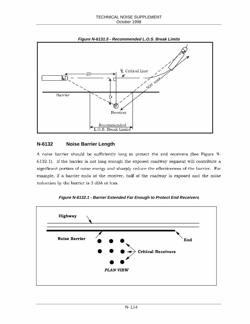
TECHNICAL NOISE SUPPLEMENTOctober 1998
N-���
Figure N-6131.5 - Recommended L.O.S. Break Limits
&/
%DUULHU
5HFHLYHU
&ULWLFDO /LQH
5HFRPPHQGHG
/�2�6� %UHDN /LPLWV
�'
8
'
���PD[�
N-6132 Noise Barrier Length
$ QRLVH EDUULHU VKRXOG EH VXIILFLHQWO\ ORQJ WR SURWHFW WKH HQG UHFHLYHUV �6HH )LJXUH 1�
�������� ,I WKH EDUULHU LV QRW ORQJ HQRXJK WKH H[SRVHG URDGZD\ VHJPHQW ZLOO FRQWULEXWH D
VLJQLILFDQW SRUWLRQ RI QRLVH HQHUJ\ DQG VKDUSO\ UHGXFH WKH HIIHFWLYHQHVV RI WKH EDUULHU� )RU
H[DPSOH� LI D EDUULHU HQGV DW WKH UHFHLYHU� KDOI RI WKH URDGZD\ LV H[SRVHG DQG WKH QRLVH
UHGXFWLRQ E\ WKH EDUULHU LV � G%$ RU OHVV�
Figure N-6132.1 - Barrier Extended Far Enough to Protect End Receivers
+LJKZD\
1RLVH %DUULHU
&ULWLFDO 5HFHLYHUV
(QG
3/$1 9,(:

TECHNICAL NOISE SUPPLEMENTOctober 1998
N-���
$V D UXOH RI WKXPE� D QRLVH EDUULHU VKRXOG H[WHQG DW OHDVW �' EH\RQG WKH ODVW UHFHLYHU�
ZKHUH ´'µ LV WKH SHUSHQGLFXODU GLVWDQFH IURP EDUULHU WR UHFHLYHU �VHH )LJXUH 1��������� 7KH
´�' UXOHµ� KRZHYHU� VKRXOG EH FRQVLGHUHG D VWDUWLQJ SRLQW DQG WKH )+:$ 0RGHO VKRXOG EH
XVHG WR H[DFWO\ ORFDWH WKH HQG RI WKH EDUULHU� 2IWHQ WKH FULWLFDO HQG UHFHLYHUV DUH QRW LQ WKH
ILUVW URZ RI KRPHV� EXW SHUKDSV VHYHUDO URZV IDUWKHU IURP WKH KLJKZD\ DV LV DOVR VKRZQ ,Q
)LJXUH 1�������� $V WKH EDUULHU WR UHFHLYHU GLVWDQFH LQFUHDVHV� WKH KLJKZD\ QRLVH EHFRPHV
OHVV� EXW WKH EDUULHU VHJPHQW DQJOH DOVR UHGXFHV� ZKLFK PDNHV D SRWHQWLDO QRLVH EDUULHU OHVV
HIIHFWLYH� 7KH )+:$ 0RGHO LV QHHGHG WR UHVROYH WKHVH RSSRVLQJ IDFWRUV�
Figure N-6132.2 - The “4D Rule”
$QRWKHU ZD\ RI GHDOLQJ ZLWK HQG UHFHLYHUV LV VKRZQ LQ )LJXUH 1�������� 7KH EDUULHU LV
´KRRNHGµ DURXQG WKH FULWLFDO UHFHLYHUV� 7KH REYLRXV DGYDQWDJH RI WKLV GHVLJQ LV WKH VKRUWHU
EDUULHU OHQJWK FRPSDUHG ZLWK WKH QRUPDO EDUULHU H[WHQVLRQ� 7KH GLVDGYDQWDJH LV WKH OHJDO
DJUHHPHQWV EHWZHHQ &DOWUDQV DQG WKH SULYDWH SURSHUW\ RZQHUV� FRQFHUQLQJ WKH FRQVWUXFWLRQ
HDVHPHQWV� EDUULHU PDLQWHQDQFH DQG UHVSRQVLELOLWLHV�
Figure N-6132.3 - Barrier Wrapped Around End Receivers, An Effective Alternative
'
� '
1RLVH %DUULHU
+LJKZD\
5HFHLYHU
(QG
PLAN VIEW
&ULWLFDO 5HFHLYHUV
1RLVH %DUULHU+LJKZD\
(QG
PLAN VIEW

TECHNICAL NOISE SUPPLEMENTOctober 1998
N-���
N-6140 Barrier Shape
6HFWLRQ 1����� LQGLFDWHG WKDW )+:$ 0RGHO GLVWLQJXLVKHV EHWZHHQ WZR QRLVH EDUULHU
VKDSHV� WKH WKLQ VFUHHQ �ZHGJH� VKDSH� DQG WKH HDUWK EHUP� )LJXUH 1����� VKRZV
UHSUHVHQWDWLRQV RI WKH WZR EDUULHU VKDSHV�
Figure N-6140.1 - Thin Screen Vs. Berm; a Berm Gives More Barrier Attenuation.
*LYHQ WKH VDPH VLWH FURVV VHFWLRQ� GLVWDQFH EHWZHHQ VRXUFH DQG UHFHLYHU� DQG EDUULHU
KHLJKW� D EHUP DOORZV D JUHDWHU EDUULHU DWWHQXDWLRQ WKDQ WKH WKLQ VFUHHQ �ZHGJH�� VXFK DV D
VRXQG ZDOO� $OWKRXJK WKH )+:$ DVVXPHV � G%$ PRUH DWWHQXDWLRQ IRU WKH EHUP WKDQ WKH
WKLQ VFUHHQ� WKH DFWXDO H[WUD DWWHQXDWLRQ PD\ EH VRPHZKHUH EHWZHHQ � DQG � G%$�
7KHUH DUH VHYHUDO SUREDEOH FDXVHV IRU WKH H[WUD � G%$ DWWHQXDWLRQ IRU D EHUP� 2QH UHDVRQ
LV WKH VKDSH RI WKH EHUP� 7KH IODW WRS DOORZV D GRXEOH GLIIUDFWLRQ� UHVXOWLQJ LQ D ORQJHU SDWK
OHQJWK GLIIHUHQFH� $QRWKHU FDXVH PD\ EH WKDW WKH QRLVH SDWK LV FORVHU WR WKH JURXQG �EHUP
VXUIDFH� WKDQ WKDW IRU D WKLQ VFUHHQ� WKXV DOORZLQJ PRUH JURXQG DEVRUSWLRQ E\ UHWDLQLQJ VRIW
VLWH FKDUDFWHULVWLFV�
2WKHU EDUULHU VKDSHV KDYH EHHQ UHVHDUFKHG� 7KHVH LQFOXGH ´7�WRSVµ� ´<�WRSV� SHDU VKDSHG
WRSV� FXUYHG ZDOOV� DQG RWKHUV� *LYHQ WKH VDPH WRWDO KHLJKW RI ZDOO� WKHVH GR OLWWOH WR
LPSURYH EDUULHU DWWHQXDWLRQ� XVXDOO\ RQO\ DERXW � RU � G%$ PD[LPXP� �)LJXUH 1�������
VKRZV VRPH GLIIHUHQW VKDSHV� 7KH H[WUD FRVW RI FRQVWUXFWLQJ WKHVH VKDSHV XVXDOO\ GRHV QRW
ZDUUDQW WKLV VPDOO EHQHILW�
7KLQ 6FUHHQ RU :HGJH
�6RXQG :DOO�
(DUWK %HUP
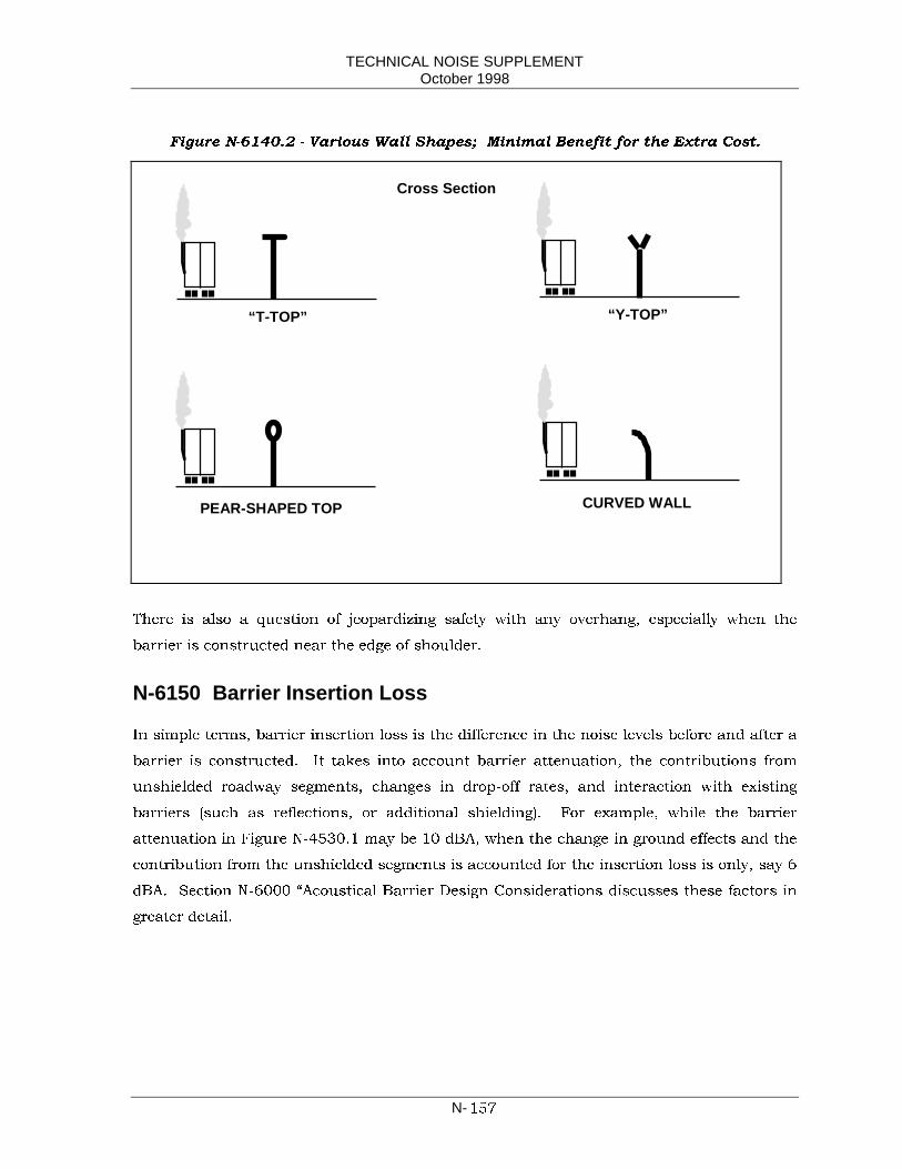
TECHNICAL NOISE SUPPLEMENTOctober 1998
N-���
)LJXUH 1������� � 9DULRXV :DOO 6KDSHV� 0LQLPDO %HQHILW IRU WKH ([WUD &RVW�
7KHUH LV DOVR D TXHVWLRQ RI MHRSDUGL]LQJ VDIHW\ ZLWK DQ\ RYHUKDQJ� HVSHFLDOO\ ZKHQ WKH
EDUULHU LV FRQVWUXFWHG QHDU WKH HGJH RI VKRXOGHU�
N-6150 Barrier Insertion Loss
,Q VLPSOH WHUPV� EDUULHU LQVHUWLRQ ORVV LV WKH GLIIHUHQFH LQ WKH QRLVH OHYHOV EHIRUH DQG DIWHU D
EDUULHU LV FRQVWUXFWHG� ,W WDNHV LQWR DFFRXQW EDUULHU DWWHQXDWLRQ� WKH FRQWULEXWLRQV IURP
XQVKLHOGHG URDGZD\ VHJPHQWV� FKDQJHV LQ GURS�RII UDWHV� DQG LQWHUDFWLRQ ZLWK H[LVWLQJ
EDUULHUV �VXFK DV UHIOHFWLRQV� RU DGGLWLRQDO VKLHOGLQJ�� )RU H[DPSOH� ZKLOH WKH EDUULHU
DWWHQXDWLRQ LQ )LJXUH 1������� PD\ EH �� G%$� ZKHQ WKH FKDQJH LQ JURXQG HIIHFWV DQG WKH
FRQWULEXWLRQ IURP WKH XQVKLHOGHG VHJPHQWV LV DFFRXQWHG IRU WKH LQVHUWLRQ ORVV LV RQO\� VD\ �
G%$� 6HFWLRQ 1����� ´$FRXVWLFDO %DUULHU 'HVLJQ &RQVLGHUDWLRQV GLVFXVVHV WKHVH IDFWRUV LQ
JUHDWHU GHWDLO�
“T-TOP” “Y-TOP”
PEAR-SHAPED TOP CURVED WALL
Cross Section

TECHNICAL NOISE SUPPLEMENTOctober 1998
N-���
Figure 6150.1 - Barrier Insertion Loss Vs. Barrier Attenuation
N-6160 Background Noise Levels2QH LPSRUWDQW IDFWRU WR EH FRQVLGHUHG �DQG RIWHQ RYHUORRNHG� LQ QRLVH EDUULHU GHVLJQ LV WKH
EDFNJURXQG QRLVH OHYHO ZLWKLQ D FRPPXQLW\� $ QRLVH EDUULHU FDQQRW UHGXFH QRLVH OHYHOV
EHORZ WKH QRLVH OHYHO JHQHUDWHG E\ ORFDO WUDIILF RQ VXUIDFH VWUHHWV ZLWKLQ D FRPPXQLW\� )RU
LQVWDQFH� LI WKH EDFNJURXQG OHYHO �ZLWKRXW WKH KLJKZD\� LV �� G%$ �DW WKH WDUJHW UHFHLYHUV��
DQG D SURSRVHG SURMHFW ZLOO UDLVH WKLV OHYHO WR �� G%$ DW WKH VDPH UHFHLYHUV� D QRLVH EDUULHU
ZLOO QRW EH DEOH WR ORZHU WKH QRLVH OHYHO GRZQ WR EHORZ �� G%$� 7KHUHIRUH� WKH FRPPXQLW\
´EDFNJURXQGµ QRLVH OHYHO VKRXOG DOZD\V EH DGGHG LQWR WKH SUHGLFWHG QRLVH OHYHOV DQG
FRQVLGHUHG LQ WKH QRLVH DWWHQXDWLRQ GHVLJQ SURFHVV� 2QO\ LI LW LV REYLRXV WKDW WKH
EDFNJURXQG QRLVH IURP ORFDO VRXUFHV ZLOO QRW LQIOXHQFH WKH QRLVH EDUULHU·V LQVHUWLRQ ORVV �L�H�
LV DW OHDVW �� G%$ EHORZ WKH SUHGLFWHG QRLVH OHYHO ZLWK WKH QRLVH EDUULHU�� FDQ WKH
EDFNJURXQG QRLVH EH LJQRUHG�
7KH IROORZLQJ WZR H[DPSOHV LOOXVWUDWHV D PHWKRG RI LQFOXGLQJ H[LVWLQJ EDFNJURXQG QRLVH
OHYHOV� 7KH ILUVW H[DPSOH LQYROYHV D QHZ IDFLOLW\ LQ D UHVLGHQWLDO DUHD� 7KH VHFRQG LQYROYHV D
SURMHFW DORQJ DQ H[LVWLQJ IDFLOLW\�
([DPSOH �� 1HZ )DFLOLW\
%DFNJURXQG QRLVH OHYHO� �� G%$ DW 5HFHLYHU�V�
1HZ IDFLOLW\ �Z�R EDFNJURXQG� �� G%$ DW 5HFHLYHU�V�
7RWDO SUHGLFWHG� �� G%$ DW 5HFHLYHU�V�
RECEIVER
NOISE BARRIER
�&KDQJH LQ *URXQG (IIHFW
GXH WR %DUULHU�
�1RLVH &RQWULEXWLRQ IURP
8QVKLHOGHG $UHD�
�1RLVH &RQWULEXWLRQ IURP
8QVKLHOGHG $UHD�
%DUULHU $WWHQXDWLRQ 1RLVH DWWHQXDWLRQ GXH WR %DUULHU �GLIIUDFWLRQ� RQO\�
%DUULHU ,QVHUWLRQ /RVV 1HW HIIHFW RI %DUULHU $WWHQXDWLRQ� FKDQJH LQ *URXQG (IIHFW�
DQG 1RLVH &RQWULEXWLRQ IURP XQVKLHOGHG DUHDV� L�H� %HIRUH � $IWHU %DUULHU 1RLVH /HYHO�
TECHNICAL NOISE SUPPLEMENTOctober 1998
N-���
)URP WKH DERYH GDWD ZH GHFLGH WR GHVLJQ D QRLVH EDUULHU WKDW ZLOO UHGXFH WKH WRWDO
QRLVH OHYHO E\ � G%$� 7KH PRGHO SUHGLFWV QRLVH OHYHOV ZLWKRXW WKH EDFNJURXQG QRLVH
OHYHO� <HW� WKH ODWWHU VKRXOG EH DFFRXQWHG IRU LQ WKH WRWDO QRLVH DWWHQXDWLRQ� 7KXV
ZH PXVW FDOFXODWH ZKDW ZKDW SUHGLFWHG QRLVH OHYHO LV QHHGHG WR UHGXFH WKH WRWDO
SUHGLFWHG QRLVH OHYHO WR �� G%$�
%DFNJURXQG QRLVH OHYHO� �� G%$ DW 5HFHLYHU�V�
3UHGLFWHG QRLVH OHYHO� "" G%$ DW 5HFHLYHU�V�
7RWDO GHVLUHG QRLVH OHYHO� �� G%$ DW 5HFHLYHU�V�
3UHGLFWHG QRLVH OHYHO �� G%$ � �� G%$ ��/RJ�� ������
������
� ����� VD\ �� G%$�
7KH FDOFXODWHG LQVHUWLRQ ORVV VKRXOG WKHQ EH �� � �� � G%$ WR UHGXFH WKH WRWDO
QRLVH OHYHO E\ � G%$�
7KH QH[W H[DPSOH� LQYROYLQJ DQ H[LVWLQJ IDFLOLW\� LV PRUH FRPSOLFDWHG� EHFDXVH WKH
EDFNJURXQG QRLVH OHYHOV DW WKH UHFHLYHUV ORFDWHG QHDU WKH H[LVWLQJ KLJKZD\ DUH
FRQWDPLQDWHG E\ QRLVH RULJLQDWLQJ IURP WKH KLJKZD\� DQG WKHUHIRUH QRW NQRZQ�
%DFNJURXQG QRLVH OHYHOV FDQ� KRZHYHU� EH HVWLPDWHG IURP PHDVXUHPHQWV WDNHQ WKURXJKRXW
WKH FRPPXQLW\ DW VLWHV IDU HQRXJK IURP WKH KLJKZD\ WR QRW EH LQIOXHQFHG E\ LW� �VHH VHFWLRQ
1������� 2QFH WKLV LV DFFRPSOLVKHG� WKH SUREOHP LV HVVHQWLDOO\ WKH VDPH DV H[DPSOH ��
([DPSOH �� ([LVWLQJ )DFLOLW\
%DFNJURXQG QRLVH OHYHO� �� G%$ DW 5HFHLYHU�V� �HVWLPDWHG�
([LVWLQJ QRLVH OHYHO� �� G%$ DW 5HFHLYHU�V� �PHDVXUHG�
([LVWLQJ QRLVH OHYHO� �� G%$ DW 5HFHLYHU�V� �FDOFXODWHG� XVLQJ WKH PRGHO��
:LWK SURMHFW QRLVH OHYHO �� G%$ DW 5HFHLYHU�V� �SUHGLFWHG� ZLWKRXW
EDFNJURXQG�
,W LV REYLRXV WKDW WKH H[LVWLQJ QRLVH OHYHO LV FRQWDPLQDWHG E\ WKH EDFNJURXQG QRLVH OHYHO�
EHFDXVH WKH GLIIHUHQFH EHWZHHQ WKH WZR LV OHVV WKDQ �� G%$ � 7KHUHIRUH� PRGHO FDOLEUDWLRQ
LV QRW DOORZHG� DQG WKH SUHGLFWHG ZLWK SURMHFW QRLVH OHYHO LV XVHG ZLWKRXW DGMXVWPHQW� DV
H[SODLQHG LQ VHFWLRQ 1����� �0RGHO &DOLEUDWLRQ� ´&DXWLRQV DQG 3LWIDOOVµ�� 7KH SUREOHP LV
WKHQ VROYHG DV VKRZQ LQ H[DPSOH ��
TECHNICAL NOISE SUPPLEMENTOctober 1998
N-���
N-6200 NON-ACOUSTICAL CONSIDERATIONS
)LQDO VHOHFWLRQV RI PDWHULDOV� ORFDWLRQV� KHLJKWV� OHQJWKV� DQG VKDSHV RI QRLVH EDUULHUV
LQFOXGH QRQ�DFRXVWLFDO FRQVLGHUDWLRQV VXFK DV VDIHW\� DHVWKHWLFV� DQG PDLQWHQDQFH�
N-6210 Safety6DIHW\ FRQVLGHUDWLRQV LQFOXGH ODWHUDO FOHDUDQFHV� VLJKW GLVWDQFH UHTXLUHPHQWV� DQG JXDUG
UDLO RU VDIHW\ VKDSH EDUULHU UHTXLUHPHQWV� 7KHVH VDIHW\ FRQVLGHUDWLRQV DUH FRYHUHG LQ
&KDSWHU ���� RI WKH +LJKZD\ 'HVLJQ 0DQXDO�
7KH 2IILFH RI 6WUXFWXUH 'HVLJQ KDV GHYHORSHG VWDQGDUG VKHHWV IRU QRLVH EDUULHUV �VRXQG
ZDOOV�� 7KHVH KDYH EHHQ GLVWULEXWHG WR WKH 'LVWULFWV� 7KH VWDQGDUG GHVLJQV LQFOXGH WKH
IROORZLQJ PDWHULDOV�
• 0DVRQU\ EORFN�
• 3UHFDVW FRQFUHWH SDQHO �ZLWK SRVW RU PRXQWHG RQ VDIHW\ VKDSHG EDUULHU��
• :RRG �SRVW DQG SODQN RU IUDPHG SO\ZRRG�
• 0HWDO �ULEEHG VWHHO��
• &RPSRVLWH EHDP �6W\URIRDP DQG ZLUH PHVK FRUH ZLWK VWXFFR H[WHULRU�
2WKHU GHVLJQV� UHWURILW WUHDWPHQWV VXFK DV QRLVH DEVRUSWLYH SDQHOLQJ� DQG DOWHUDWLRQV WR
QRLVH EDUULHUV VKRXOG EH DSSURYHG E\ WKH 2IILFH RI 6WUXFWXUH 'HVLJQ�
7KH VWDQGDUG VKHHWV DOVR LQFOXGH GHVLJQV IRU JDWHV SURYLGLQJ HPHUJHQF\ DFFHVV WR
FRPPXQLW\ ILUH K\GUDQWV� HPHUJHQF\ DFFHVV IRU VWUDQGHG PRWRULVWV� UDSLG DFFHVV WR
DFFLGHQWV� HWF�
$ PLQLPXP KHLJKW UHTXLUHPHQW RI ��� P �� IW� IRU VRXQG ZDOOV LQ &KDSWHU ���� RI WKH
+LJKZD\ 'HVLJQ 0DQXDO ZDV SDUWLDOO\ GHVLJQHG WR FRQWURO SHGHVWULDQ DFFHVV WR WKH IUHHZD\�
N-6220 Aesthetics
7KH YLVXDO LPSDFW RI QRLVH EDUULHUV RQ DGMRLQLQJ FRPPXQLWLHV� DV ZHOO DV RQ WKH PRWRULVWV LV
D PDMRU FRQVLGHUDWLRQ LQ WKH GHVLJQ RI QRLVH EDUULHUV� $ KLJK QRLVH EDUULHU SODFHG FORVH WR
VLQJOH VWRU\ UHVLGHQFHV FRXOG KDYH D VHYHUH YLVXDO HIIHFW� $ KLJK EDUULHU FDQ DOVR FUHDWH
XQZDQWHG VKDGRZV� LPSHGH QDWXUDO DLU IORZV� RU EORFN SDQRUDPLF YLHZV� &KDSWHU ���� RI
WKH +LJKZD\ 'HVLJQ 0DQXDO RXWOLQHV PD[LPXP KHLJKWV IRU QRLVH EDUULHUV ORFDWHG DW
GLVWDQFHV RI ��� P ��� IW� RU OHVV DQG PRUH WKDQ ��� P IURP WKH WUDYHOHG ZD\�
TECHNICAL NOISE SUPPLEMENTOctober 1998
N-���
,Q JHQHUDO� YLVXDO GRPLQDQFH RI KLJK ZDOOV QHDU UHVLGHQFHV LV UHGXFHG ZKHQ WKH VRXQG ZDOO
LV ORFDWHG DW OHDVW � � � WLPHV LWV KHLJKW IURP WKH QHDUHVW UHFHLYHU� 7KH YLVXDO LPSDFW LV
IXUWKHU VRIWHQHG ZLWK EHUPV DQG ODQGVFDSLQJ �VHH )LJXUH 1��������� /DQGVFDSHG HDUWK
EHUPV DUH DFRXVWLFDOO\ DQG DHVWKHWLFDOO\ VXSHULRU WR VRXQG ZDOOV� +RZHYHU� LQ PDQ\
ORFDWLRQV WKH\ DUH QRW VXLWDEOH EHFDXVH RI VSDFH OLPLWDWLRQV�
6RXQG ZDOOV VKRXOG QRW KDYH DEUXSW EHJLQQLQJV RU HQGLQJV� ,QVWHDG WKH\ VKRXOG EH WDSHUHG
RU VWHSSHG� 2QO\ VWDQGDUG DHVWKHWLF WUHDWPHQWV GHYHORSHG E\ WKH 2IILFH RI 6WUXFWXUH 'HVLJQ
VKRXOG EH XVHG� ,I ODQGVFDSLQJ LV WR EH SODFHG DGMDFHQW WR WKH VRXQG ZDOO ZKHUH LW ZLOO
HYHQWXDOO\ VFUHHQ D VXEVWDQWLDO SRUWLRQ RI WKH ZDOO� RQO\ PLQLPDO DHVWKHWLF WUHDWPHQW LV
MXVWLILHG�
:DOOV VKRXOG DV PXFK DV SRVVLEOH UHIOHFW WKH FKDUDFWHU RI WKH VXUURXQGLQJV� ,Q FDVHV ZKHUH
WKH JHQHUDO DUFKLWHFWXUH RI D FRPPXQLW\ KDV D FHUWDLQ FKDUDFWHU� VRXQG ZDOO PDWHULDO�
WH[WXUH DQG FRORU VKRXOG SUHIHUDEO\ ILW WKLV FKDUDFWHU DW WKH FRPPXQLW\ VLGH RI WKH ZDOO�
,GHDOO\� WKH FRPPXQLW\ VKRXOG KDYH VRPH LQSXW LQ WKH DHVWKHWLF GHVLJQ RI QRLVH EDUULHUV�
2Q WKH PRWRULVW VLGH RI WKH ZDOO WKH HPSKDVLV VKRXOG EH RQ WKH RYHUDOO IRUP RI WKH ZDOO� LWV
FRORU DQG WH[WXUH� 6PDOO GHWDLOV ZLOO QRW EH QRWLFHG DW QRUPDO KLJKZD\ VSHHGV� ,QVWHDG� WKH
HPSKDVLV VKRXOG EH RQ DYRLGLQJ D WXQQHO HIIHFW WKURXJK YDULRXV IRUPV� DQG YLVXDO
WUHDWPHQWV� /DQGVFDSLQJ FDQ EH XVHG HIIHFWLYHO\ WR DFFRPSOLVK WKLV�
)XUWKHU JXLGDQFH RQ DHVWKHWLFV FDQ EH IRXQG LQ &KDSWHU ���� LQ WKH +LJKZD\ 'HVLJQ
0DQXDO� DQG �,QVWUXFWLRQV IRU XVLQJ WKH 6WDQGDUG $HVWKHWLFV )HDWXUHV 6KHHWV�� 7KH ODWWHU LV
DYDLODEOH IURP WKH $HVWKHWLFV DQG 0RGHOV XQLW RI WKH 2IILFH RI 6WUXFWXUH 'HVLJQ�

TECHNICAL NOISE SUPPLEMENTOctober 1998
N-���
Figure N-6220.1 - Spatial Relationship of Barrier to Adjoining Land Use
/HVV WKDQ ��� +
+
8QGHVLUDEOH %DUULHU 5HODWLRQVKLS
%DUULHU %HFRPHV 9LVXDOO\ 'RPLQDWLQJ�3RWHQWLDO 6KDGRZ 3UREOHPV�9LHZV 2EVFXUHG
9LVXDO 'RPLQDQFH 5HGXFHG�/DQGVFDSLQJ )XUWKHU 5HGXFHV%DUULHU ,PSDFW
+
$FFHSWDEOH %DUULHU 5HODWLRQVKLS
� ² � +
+
'HVLUDEOH %DUULHU 5HODWLRQVKLS
� RU PRUH +� WR � :DOO LQ 6FDOH
:LWK %XLOGLQJ
%HUP� /DQGVFDSLQJ6RIWHQ %DUULHU ,PSDFW
N-6230 Maintenance$FFHVV WR WKH EDFN VLGH RI QRLVH EDUULHUV PXVW EH SURYLGHG LI WKH DUHD LV PDLQWDLQHG E\
&DOWUDQV� ,I DFFHVV LV QRW DYDLODEOH IURP ORFDO VWUHHWV DFFHVV JDWHV RU RSHQLQJV IURP WKH
KLJKZD\ PXVW EH SURYLGHG DORQJ WKH QRLVH EDUULHU� 2SHQLQJV FUHDWHG E\ RYHUODSSLQJ
EDUULHUV PXVW KDYH DQ RYHUODS GLVWDQFH RI DW OHDVW ��� WR � WLPHV WKH ZLGWK RI WKH RSHQLQJ
�GLVWDQFH EHWZHHQ RYHUODSSLQJ EDUULHUV� �VHH )LJXUH 1���������
Figure N-6230.1 - Barrier Overlap 2.5 to 3 times the Width of the Access Opening.
a
2.5 to 3 a
FREEWAY
Noise Barrier @ R/WNoise Barrier @ Shoulder
TECHNICAL NOISE SUPPLEMENTOctober 1998
N-���
7KH DOWHUQDWH PDWHULDOV VHOHFWHG IRU QRLVH EDUULHUV VKRXOG EH DSSURSULDWH IRU WKH
HQYLURQPHQW LQ ZKLFK WKH\ DUH SODFHG� )RU LQVWDQFH� IRU ZDOOV WKDW DUH ORFDWHG QHDU WKH HGJH
RI VKRXOGHU� WKH PDWHULDO DERYH WKH VDIHW\�VKDSH FRQFUHWH EDUULHU VKRXOG EH DEOH WR
ZLWKVWDQG WKH LPSDFW RI DQ RFFDVLRQDO YHKLFOH ULGLQJ XS DERYH WKH WRS RI WKH VDIHW\ EDUULHU�
&RQFUHWH EORFN� FDVW�LQ�SODFH FRQFUHWH� RU SUHFDVW FRQFUHWH SDQHOV DUH UHFRPPHQGHG LQ
WKHVH ORFDWLRQV� ,Q DUHDV RI JUHDW ILUH GDQJHU� ZRRG EDUULHUV VKRXOG EH DYRLGHG� 6HH &KDSWHU
���� RI WKH +LJKZD\ 'HVLJQ 0DQXDO IRU IXUWKHU LQIRUPDWLRQ�

TECHNICAL NOISE SUPPLEMENTOctober 1998
N-���

TECHNICAL NOISE SUPPLEMENTOctober 1998
N-165
N-7000 NOISE STUDY REPORTSThe primary function of a noise study report is to present the methods and results of a
traffic noise analysis and the data supporting the conclusions to a target audience that
includes both lay persons and technical noise analysts. One way to satisfy both
audiences is to provide a summary for lay persons and decision makers, and a technical
report for experienced noise analysts, or lay persons desiring more detail than that
provided by the summary.
The summary, also called the Executive Summary, should briefly describe existing
landuse and noise environment, the project alternatives, future noise environment, traffic
noise impacts (if any) and noise abatement/mitgation considered.
The technical report needs to fully support the conclusions that are incorporated into the
environmental document and should satisfy technical reviewers who wish to assess the
validity of the noise study, including the methods used as well as any assumptions that
have been made. Sufficient information should be presented to allow any trained noise
analyst to come to the same conclusions.
As is the case with all technical environmental studies, the level of effort to be spend on
the noise study report needs to be matched with the size and complexity of the project,
and degree of controversy (if any) surrounding it.
N-7100 OUTLINETable N-7100-1 shows an outline for a typical noise study report. Not all reports will need
this level of effort. On the other hand, some reports may require more information due to
special circumstances.
Table N-7100-1 Noise Study Report Outline
I. SUMMARY (OR EXECUTIVE SUMMARY)• Purpose of noise report• Brief description of the project• Brief description of the land use and terrain• Existing noise levels (ambient and background)• Future predicted noise levels• Traffic noise impacts (if any)• Noise abatement/mitigation considered (range of heights, lengths, insertion
losses, and no. of benefited receivers• Reasonable monetary allowances per benefited receiver for abatement
considered• Areas where abatement/mitigation are not feasible

TECHNICAL NOISE SUPPLEMENTOctober 1998
N-166
• Construction noise
Table N-7100-1 Noise Study Report Outline (continued)
II. NOISE IMPACT TECHNICAL REPORTA. Introduction
1. Purpose of report2. Background
B. Project Description1. Detailed description of all project alternatives2. Maps showing alignment and profiles
C. Fundamentals of Traffic Noise1. Decibels and frequency2. Noise source characteristics (vehicles & roadways)3. Noise propagation4. Perception at the receiver, A-weighting, noise descriptors5. Decibel scale
D. Federal & State Policies and Procedures1. Traffic Noise Analysis Protocol2. Technical Noise Supplement
E. Study Methods and Procedures1. Selection of receivers and measurement sites2. Field measurement procedures: (Note: field data in appendices)
a. instrumentation and setupsb. noise measurementsc. traffic counts and speedsd. meteorologye. data reduction
3. Noise prediction method used:a. LEQV2 or SOUND32 based on FHWA RD-77-108 Report and Calveno
(FHWA/CA/TL-87/03) Report, orb. TNM, based on FHWA-PD-96-009 and – 010 (when mandated)
F. Existing Noise Environment1. Detailed description of noise sensitive land use2. Maps showing receivers and noise measurement sites3. Table showing existing noise levels at receivers:
a) Field measured results (ambient and background)b) Modeled results
4. Discussion on model calibration (if appropriate) for adjusting modeled noiselevels (existing or future)
G. Future Noise Environment, Impacts, and Cosidered Abatement/Mitigation1. Discuss future traffic data assumptions and site geometry2. Table showing predicted noise levels, and identification of traffic noise
impacts, if any3. Discussion of noise abatement options

TECHNICAL NOISE SUPPLEMENTOctober 1998
N-167
4. Table showing future noise levels and insertion losses (noise reduction) forvarious noise barrier heights, lengths and locations
5. Table summarizing data necessary for “Reasonableness” determination6. Discussion of areas where abatement/mitigation is not feasible
Table N-7100-1 Noise Study Report Outline (continued)H. Construction NoiseI. ReferencesJ. Appendices
1. Instrumentation, manufacturer(s),model, type, serial numbers, calibration2. Measurement site details, instrument setups3. Measurement procedures, duration, number of repetitions4. Measured noise data, dates, times5. Meteorological conditions6. Traffic counts7. Data reduction, measurement results8. Details of computer modeling assumptions, inputs and outputs
N-7200 SUMMARY (OR EXECUTIVE SUMMARY)The noise study conclusions should be presented near the front of the Noise Study Report
in the form of a summary, also called Executive Summary. The summary of findings and
conclusions of the study should be extracted from the technical portion of the noise study
report. This requires the technical portion to be written first. The executive summary
should target the layperson who is interested in the noise impacts, if any, but does not
want to read all of the technical details. Because the author of the Noise Study Report is
usually not the same author of the project’s environmental document, the executive
summary should be written in such a manner, that it can be “cut and pasted” into the
environmental document. This will help reduce misinterpretations or loss in translations.
The Executive Summary should be short, usually only a few pages. Briefly describe the
elements mentioned in the outline (Table N-7100-1). A table listing receivers, existing
noise levels, future noise levels without noise barriers, future noise levels with noise
barriers (various heights), and insertion loss should be sufficient to summarize the results
of the noise study.
N-7300 NOISE IMPACT TECHNICAL REPORTThe noise impact technical portion is the main body of the Noise Study Report. It contains
detailed descriptions of why and how the noise study was performed and how the
conclusions were reached. Sufficient detail is needed for someone to be able to duplicate
the study from the information included in report.

TECHNICAL NOISE SUPPLEMENTOctober 1998
N-168
Depending on the size, location and type of project, it may be beneficial to combine the
noise report with some of the other technical reports, such as air quality, in order to avoid
repetition.
Following are suggested sections of the report with brief descriptions of their contents.
N-7310 IntroductionThe introduction should include the purpose of the Noise Study Report, study objectives,
and background information such as need for project and need for the study, or any other
general information useful to the understanding of the Noise Study Report.
N-7320 Project DescriptionThe project description should include a detailed description of all of the project
alternatives. There should be enough information for the reader to understand the project
and how it fits into the transportation system of the area. An appropriate location map
showing alternative alignments studied and and their spatial relationship with noise
sensitive receivers such as residences, schools, hospitals, churches and parks should be
included.
N-7330 Fundamentals of Traffic NoiseA short review of the physical principles of traffic noise at the source and its propagation,
and subjective human perception will provide a link for lay persons to understand the
technical information. The contents of this section may be of standard format or tailored
to specific studies.
Briefly describe sound pressure level, the logarithmic nature of decibel units, and
frequency (pitch), and the noise characteristics of vehicles. Vehicle noise emissions
increase with speed. Increased traffic volumes also increase traffic noise. However it
takes a doubling of traffic to increase noise levels by only 3 dB.
Discuss the noise propagation (line source vs point source) over acoustically “hard” and
“soft” ground, effects by meteorolgical factors such as wind and temperature gradients,
shielding by terrain or noise barriers.
Human perception of noise is also frequency dependent, which leads to a discussion on
“A-weighting”, its purpose and its use. Changes in noise levels are perceived as follows: 3
dBA barely perceptible, 5 dBA readily perceptible, and 10dBA perceived as a doubling or
halving of noise. Follow this with a discussion on commonly used noise descriptors, such
as Leq(h).

TECHNICAL NOISE SUPPLEMENTOctober 1998
N-169
Finally, the inclusion of a decibel scale showing a link between everyday activities and
associated noise levels will provide the reader with a “yard stick” to evaluate the severity
of traffic noise.
The fundamentals of traffic noise discussion need not be restricted to the above items.
Other topics may be included as appropriate, some of which may be specifically tailored to
the nature of the noise study. The information presented in this TeNS may be beneficial
in explaining various phenomena. For instance, where parallel or single noise barrier
noise reflections are an issue, it may prove to be beneficial to include selected text of
section N-8000, Special Considerations.
N-7340 Federal & State Standards and PoliciesThis section covers the applicable Federal and State standards and policies. Caltrans
noise analysis policies are in the Traffic Noise Analysis Protocol and the Highway Design
Manual Federal requirements include NEPA and 23CFR772. State requirements and
policies are contained in CEQA, California Streets and Highways Code Section 216, and.
Terms used in the policies and standards should be mentioned in this section along with
the Noise Abatement Criteria (NAC) and their significance, definitions of appropriate noise
descriptors, and traffic noise impact criteria.
If the project involves local noise ordinances written in terms of a noise descriptor other
than Leq(h) an attempt should be made to equate the noise descriptors rather than
duplicating most of the noise report using another descriptor (see Section N-2230 for a
discussion of equating worst-hour Leq's to Ldn's, etc.).
N-7350 Study Methods and ProceduresStudy methods and procedures followed should be identified in the Noise Study Report.
This section should describe selecting receivers and noise measurement sites, field
measurement procedures, and noise prediction methods (Sections N-3000 and N-5000).
The discussion of selecting the receivers and noise measurement sites should focus on
why they were selected. Selections are based on expectations of worst noise impacts,
geometry of the project, representativeness, acoustical equivalence, and human use
(Sections N-3200 and N-5310). The importance of selecting receivers outside the area of
project influence must not be overlooked. These receivers are extremely useful for
documenting background noise levels and – later, after the project is built - guard against
unsubstantiated public claims that noise barriers constructed as part of the project
increased noise levels at distant receivers (Section N-8200).

TECHNICAL NOISE SUPPLEMENTOctober 1998
N-170
The discussion on field measurement procedures (Section N-3000) should include
descriptions of instrumentation, set-ups, noise measurement procedures, traffic counts
and speeds, meteorological observations and data reduction methods. Also discuss model
calibration procedures (Section N-5400).
Include in the appendices to the noise report the measurement equipment used,
calibration information and dates and times of measurements, and measured noise data,
traffic counts and speeds, meteorological conditions, site topography, and detailed
measurement locations (as a rule of thumb, the microphone locations should be
retraceable within one meter horizontally, and 0.3 meter vertically). If measurements were
taken at a time different from the worst noise hour, show the adjustment and procedure
used (Section N-3312), any receivers modeled and calibrated, and the inputs for these.
Noise level predictions must be based on the methodology in the FHWA Highway Traffic
Noise Prediction Model (FHWA-RD-77-108) with California reference energy mean
emission (Calveno) levels, or when implemented for use by Caltrans the FHWA Traffic
Noise Model (FHWA-PD-96-009 & -010; DOT-VNTSC-FHWA-98-1 & -2),. These, and other
documents pertinent to the noise study should be referenced, as appropriate.
N-7360 Existing Noise EnvironmentBefore traffic noise impacts can be evaluated, a detailed knowledge of the existing noise
environment is required. A description of the project’s surrounding land use (residential,
commercial zones, undeveloped land, farm land etc.) should be included in this section.
The number and type of receivers involved should be reported so that the reader
understands the size and charcteristics of the area under study (e.g. “… .approximately 75
first tier single family residences; 5 two-story apartments; 2 grammar schools and 3
parks… ” etc. Mention any particularly sensitive land uses. For undeveloped land include
future uses if known. Also note the presence of any ather stationary or mobile noise
sources, e.g. arterials, airports, etc.
The general topography surrounding the project and any problems in noise measurements
or modeling should be pointed out in this section, especially in complicated or unusual
situations. A discussion on background noise levels, noise levels unaffected by the
existing highway, is also appropriate. The importance of selecting measurement sites to
document background noise levels is mentioned in the previous section N-7350.
For each receiver selected for the noise impact analysis, show:
• location or address• type of development

TECHNICAL NOISE SUPPLEMENTOctober 1998
N-171
• the number of units represented by the receiver• landuse activity category and Noise Abatement Criterion• existing noise level results (“raw” data should go into appendices)• whether existing noise level was measured or modeled (predicted); if measured, also
indicate if measurement was adjusted to worst hour noise (see Section N-3312); whenpredicted, indicate if prediction included model calibration (see Section 5400; thedetails

TECHNICAL NOISE SUPPLEMENTOctober 1998
N-172
of the calibration, such as the calibration constant and any explanations of why theywere excessiveley large, should be in the appendices).
Table N-7360.1 suggests how the information might be displayed in tabular form. The format
shown is only an example. The information may be presented in many other ways, as long as
the result is clear, concise and effective.
This section should only show a summary of the results. It is important to mention whether
the existing noise levels reflect the worst noise hour, or other time periods. The text should
include brief discussions on meteorological conditions during measurements, and
meteorological criteria. “Raw” data of noise measurements, traffic counts, speeds,
meteorological, site locations and topography should be included in the appendices.
N-7370 Future Noise Environment, Impacts, and ConsideredAbatement/ Mitigation
This section of the Noise Study Report deals with the future noise environment. A discussion
of the assumptions and inputs used for the predicted noise levels is appropriate. Include the
source of predicted future traffic volumes (such as: from traffic models, assumed level of
service C or D, design hour traffic, etc.), vehicle mix, and speeds. The actual input/output
data should be presented in the appendices.
The predicted results for future noise levels, traffic noise impacts, and considered abatement,
if any, should be presented in a clear and concise manner. As was shown in Section N-7360,
the summary information is most often best displayed in tables. An example of presenting
predicted noise levels and impacts is shown in Table N-7370.1. The table shows receivers,
receiver type, location, and or address, existing noise levels, predicted noise levels, noise
increase or decrease, activity category, NAC, and impact type. Include a project map showing
receivers and approximate locations of noise barrier locations considered.
The predicted noise and impact results table covers information for discrete receivers. The
information must be expanded to include the entire study area. Table N-7360.1 in the
previous section showed how many units were represented by each of the selected receivers.
This information can be used to identify areas of traffic noise impacts and the acoustical
design of noise barriers, (e.g. length, height, insertion loss). For projects where traffic noise
impacts have been identified, show heights and lengths of all feasible noise barriers or other
abatement measures, and enough information to determine the reasonable noise abatement
allowance per benefitted residence for each noise barrier and height considered. The latter is
necessary to determine whether abatement measures are reasonable. Although noise barriers
are normally considered for abatement/mitigation, other measures may also be considered
(see Protocol, Sec. 5.2), and in some instances a better option.
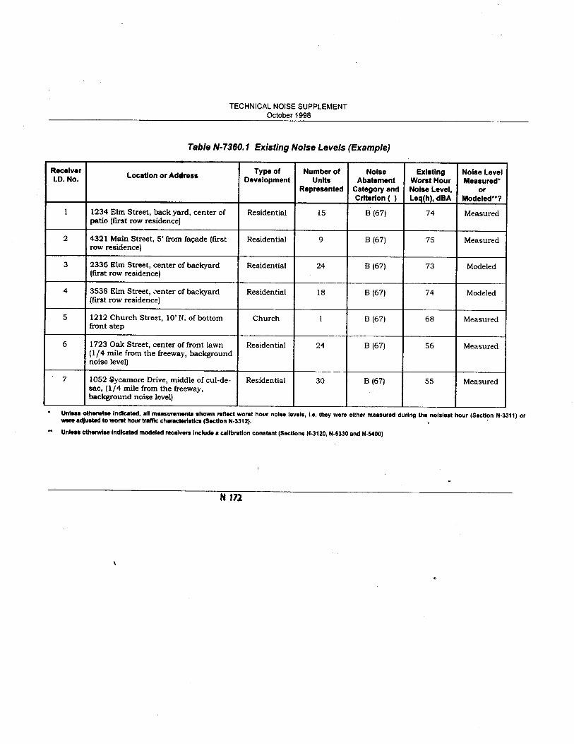

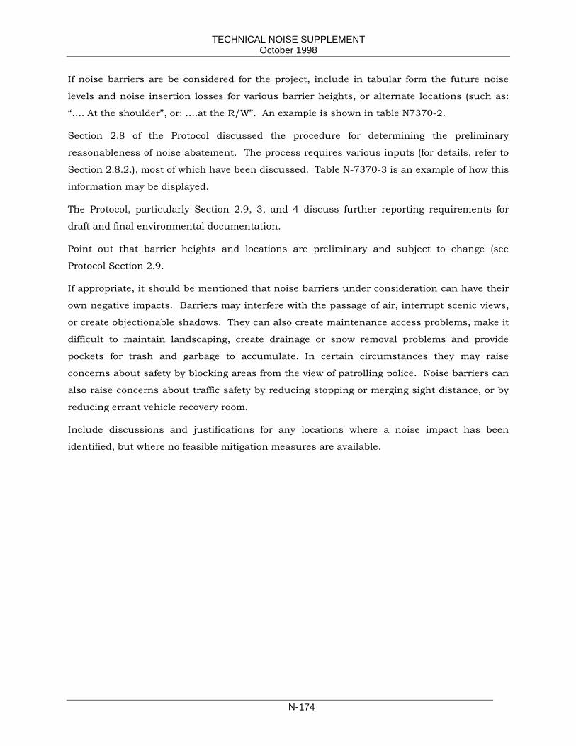
TECHNICAL NOISE SUPPLEMENTOctober 1998
N-174
If noise barriers are be considered for the project, include in tabular form the future noise
levels and noise insertion losses for various barrier heights, or alternate locations (such as:
“… . At the shoulder”, or: … .at the R/W”. An example is shown in table N7370-2.
Section 2.8 of the Protocol discussed the procedure for determining the preliminary
reasonableness of noise abatement. The process requires various inputs (for details, refer to
Section 2.8.2.), most of which have been discussed. Table N-7370-3 is an example of how this
information may be displayed.
The Protocol, particularly Section 2.9, 3, and 4 discuss further reporting requirements for
draft and final environmental documentation.
Point out that barrier heights and locations are preliminary and subject to change (see
Protocol Section 2.9.
If appropriate, it should be mentioned that noise barriers under consideration can have their
own negative impacts. Barriers may interfere with the passage of air, interrupt scenic views,
or create objectionable shadows. They can also create maintenance access problems, make it
difficult to maintain landscaping, create drainage or snow removal problems and provide
pockets for trash and garbage to accumulate. In certain circumstances they may raise
concerns about safety by blocking areas from the view of patrolling police. Noise barriers can
also raise concerns about traffic safety by reducing stopping or merging sight distance, or by
reducing errant vehicle recovery room.
Include discussions and justifications for any locations where a noise impact has been
identified, but where no feasible mitigation measures are available.

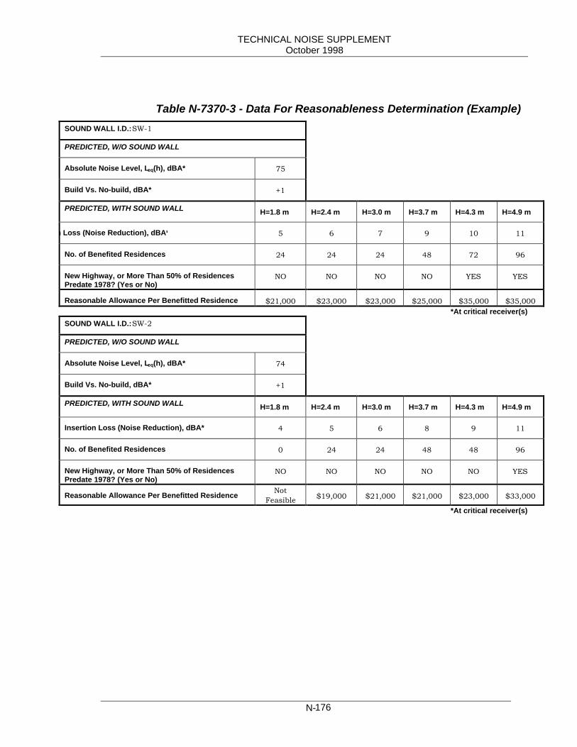
TECHNICAL NOISE SUPPLEMENTOctober 1998
N-176
Table N-7370-3 - Data For Reasonableness Determination (Example)SOUND WALL I.D.: SW-1
PREDICTED, W/O SOUND WALL
Absolute Noise Level, Leq(h), dBA* 75
Build Vs. No-build, dBA* +1
PREDICTED, WITH SOUND WALL H=1.8 m H=2.4 m H=3.0 m H=3.7 m H=4.3 m H=4.9 m
n Loss (Noise Reduction), dBA* 5 6 7 9 10 11
No. of Benefited Residences 24 24 24 48 72 96
New Highway, or More Than 50% of ResidencesPredate 1978? (Yes or No)
NO NO NO NO YES YES
Reasonable Allowance Per Benefitted Residence $21,000 $23,000 $23,000 $25,000 $35,000 $35,000*At critical receiver(s)
SOUND WALL I.D.: SW-2
PREDICTED, W/O SOUND WALL
Absolute Noise Level, Leq(h), dBA* 74
Build Vs. No-build, dBA* +1
PREDICTED, WITH SOUND WALL H=1.8 m H=2.4 m H=3.0 m H=3.7 m H=4.3 m H=4.9 m
Insertion Loss (Noise Reduction), dBA* 4 5 6 8 9 11
No. of Benefited Residences 0 24 24 48 48 96
New Highway, or More Than 50% of ResidencesPredate 1978? (Yes or No)
NO NO NO NO NO YES
Reasonable Allowance Per Benefitted Residence NotFeasible $19,000 $21,000 $21,000 $23,000 $33,000
*At critical receiver(s)

TECHNICAL NOISE SUPPLEMENTOctober 1998
N-177
N-7380 Construction Noise
Construction noise impacts and likely abatement measures thereof (if necessary) should
be discussed briefly. Unless the project involves construction activities that are likely to
generate unusually high noise levels such as pile driving or pavement breaking, the
discussion should be brief and concise. Detailed discussions of typical construction
equipment noise levels are probably not necessary unless there are unusually sensitive
receptors involved, or if the project is controversial.
N-7390 References
Typical references may include NEPA, CEQA, 23 CFR 772, Traffic Noise Analysis Protocol
Highway Design Manual Chapter 1100, FHWA-RD-77-108 or (when TNM is mandated)
FHWA-PD-96-009 & -010, DOT-VNTSC-FHWA-98-1 & -2, and other appropriate
documents.
N-7400 APPENDICESInclude in the appendices any details that would support the conclusions of the Noise
Study Report. Examples are instrumentation used, calibration data, field measurement
data, site details and computer modeling input assumptions and results. If the analysis
includes model calibrations (Section N-5400) these should be shown in simple table form
(see Table 7340.1) Ideally the appendicies should fill in all of the details that are not in
the main report such that the analysis could be repeated.
Table N-7340.1 Model Calibration (Example)Receiver
I.D.Measured
NoiseLevel,Leq(h),
dBA
PredictedNoiseLevel,Leq(h),
dBA
Calibration
Constant,K
(Meas-Pred), dBA
1 68 70 -2
2 66 69 -3
3 70 71 -1
4 69 72 -3

TECHNICAL NOISE SUPPLEMENTOctober 1998
N-178
If measurements were taken at a time different from the worst noise hour, show the
adjustment and procedure used (Section N-3312), any receivers modeled and calibrated,
and the inputs for these.

TECHNICAL NOISE SUPPLEMENTOctober 1998
N-179
N-8000 SPECIAL CONSIDERATIONSThis chapter is devoted to special considerations arising from certain site geometries, noise
barrier configurations, intervening terrain, distant receivers, interactions with meteorology,
and abnormal traffic conditions. Any one or more of these factors can affect noise
measurements, analysis, and barrier design, with results that are predicted with more than
routine methods.
Continuing research by Caltrans and others have provided some answers to these
problems. However, there is a continued need for field research to verify prediction
algorithms in new prediction models, alter those in existing ones, and investigate
conditions which lead to newly identified problems.
The "special considerations" covered in this chapter include reflected noise and noise
barriers, distant receivers, multiple barriers, and dealing with stop-and-go traffic.
N-8100 REFLECTED NOISE AND NOISE BARRIERS
Section N-6100 "Acoustical Design Considerations" briefly discussed the possibility of noise
reflections by a single noise barrier causing noise problems at the opposite side of the
highway. This is just one of the issues raised in recent years concerning negative effects of
noise barriers. As is often the case, the solution of one problem gives rise to the possibility
of creating other problems. In the case of noise barriers, reducing noise at receivers on one
side of the highway could potentially increase the noise at receivers on the other side. The
complex nature of noise barrier reflections, the difficulties in measuring them, and the
controversy surrounding the significance of their impacts deserve a detailed discussion.
More noise barriers have been constructed in California than in any other state, in many
different configurations of alignment, profile, and height. These barriers are located along
one or both sides of highways of different widths, along ramps, connectors and
interchanges, in urban, suburban, and sometimes rural regions under varying traffic
conditions. The receivers for which they were designed are located in many different types
of terrain, topography, and climatic conditions. The combinations and permutations
associated with the vast variety of conditions inevitably increase the possibilities of creating
controversies over the extent of noise reflections by barriers. Hence, it is only natural that
noise reflection issues are on the rise in California, especially since almost all California
barriers are made of noise reflective material with hard, relatively smooth surfaces
(masonry, concrete). In most cases, the alleged noise increases due to reflections turn out
to be so small that most people do not notice them. The people that do perceive increases

TECHNICAL NOISE SUPPLEMENTOctober 1998
N-180
in noise are usually suddenly made aware of freeway noise by some event that triggers the
awareness, such as the construction of the noise barrier. Measured increases due to noise
reflections of more than 2 dBA have never been measured by Caltrans, however, claims of
10 and even 20 dBA increases have occasionally been made.
Many of the alleged increases in noise were actually due to changes in meteorology.
Atmospheric refraction due to wind shear and temperature gradients can account for 10 to
15 dBA variations when the same sources are measured from distances of 1.5 to 3 km
(approximately 1 to 2 miles). In order to measure the effects of noise reflections, before and
after barrier noise measurements have to be carefully matched by wind speed, wind
direction, temperature gradients, air temperature, humidity, and sky cover. Likewise, if a
person perceives a noticeable increase in noise levels due to a reflective noise barrier,
he/she must be able to compare it mentally with a before condition that included the same
meteorology. Needless to say, this process is very unreliable.
Section 8100 covers various aspects of noise reflection concerns in detail. The following
classifications of reflective noise with respect to noise barriers and other structures will be
discussed:
1. Single barrier (on one side of a highway)
2. Parallel barriers (on both sides of the highway)
3. Structures and canyon effects
When compared to reflections measured under similar conditions, results of theoretically
modeled noise reflections normally show higher values. This over prediction of reflection
models has been attributed to the inability of models to accurately account for all the
variables, such as interactions with atmospheric effects and the unknown degree to which
traffic streams interfere with reflections.
Reflective noise is not peculiar to noise barriers. Retaining walls and other structures
reflect noise in the same manner as noise barriers do. The principles discussed in this
section can be applied to reflective barriers, reflective retaining walls, or any other smooth,
continuous and hard surface.

TECHNICAL NOISE SUPPLEMENTOctober 1998
N-181
N-8110 Single Barrier Reflections
N-8111 Simple Terrain
Figure N-8111.1 is the simplest, two-dimensional representation of single barrier
reflections. The presence of a reflective barrier on the opposite side of an at-grade highway
essentially doubles the acoustic energy at the receiver. In addition to the direct noise "ray"
"d", the barrier reflects a noise ray "r" of roughly the same acoustic energy (actually ”r” is
longer than “d” and will result in slightly less acoustical energy). Theoretically, only one
reflective ray reaches the receiver, because the angle of incidence equals the angle of
reflection (both are depicted as ? in Figure N-8111.1). Thus, even if they are equal, “r” and
“d” cause a doubling of energy increases the noise level by 3 dB at the receiver.
Figure N-8111.1 - Single Barrier Reflection (Simplest Representation)
Figure N-8111.2 shows that for an infinite line source and noise barrier the reflections are
also an infinite line source. At each point along the highway there is only one reflection ray
that reaches the receiver and for which the angle of incidence equals the angle of reflection.
Figure N-8111.2 – Single Barrier Reflections – Infinite Line Source and Noise Barrier
Cross Sectional View
Noise Barrier
Source(Highway)
r
d
?
?
Receiver
Plan View
Noise Barrier
Sources (Highway)
Receiver

TECHNICAL NOISE SUPPLEMENTOctober 1998
N-182
Figure N-8111.3 is a more realistic depiction, which includes pavement reflections. Note,
however, that a noise barrier on the opposite side still increases the noise level by 3 dB,
although the before and after noise levels are 3 dB higher (due to the pavement reflections)
than in Figures N-8111.1 and N-8111.2. In plan view, the pavement reflections would also
shown to be a line source.
The reflection point R1, shown on the pavement (Figure N-8111.3) may actually fall off the
pavement on absorptive ground, reducing the before barrier noise levels at the receiver.
The pavement reflection point R2, however, significant only after building the barrier, will
usually be on the pavement. The difference between before and after barrier noise levels
could therefore slightly exceed 3 dBA.
Figure N-8111.3 - Single Barrier Reflection (More Accurate Representation)
The effects of single noise barrier reflections are distance dependent. At distant receivers,
the ratios of direct/reflected noise path lengths as well as those for near/far lane distances
approach 1. When this is the case, contributions of direct and reflected noise from each
lane contributes roughly the same energy (of course there will always remain a slight loss of
acoustical energy due to imperfect reflections), with the result that the increase approaches
3 dBA for distant receivers. For receivers close to the highway, however, the distance ratios
become less than 1 and the noise at the receiver is dominated by direct noise from the near
lanes. The result is less contribution from reflected noise.
Figure N-8111.4 shows the distance dependency of the noise increases due to the barrier
reflections, for a typical 8-lane at-grade freeway. At 15 m (50 ft) from the edge of the
traveled way (ETW) the increase is only 1.3 dBA; at 60 m (200 ft) the increase is 2.0 dBA,
and at 120 m (400 ft) from the ETW the increase is 2.4 dBA. The increases were calculated
Cross Sectional View
Noise Barrier
Source(Highway)
R1R2

TECHNICAL NOISE SUPPLEMENTOctober 1998
N-183
assuming equal noise source distributions in the near and far (E/B and W/B) lanes, and
hard site propagation.
Figure N-8111.4 - Noise Increases due to Single Barrier Reflections.
Actually, the "real world" is far more complicated than shown in figures N-8111.1 through
N-8111.4. Consider that the noise sources are distributed over the width of the highway;
that the paths of the barrier noise reflections are always longer than the direct noise paths;
that reflective barriers are not perfect reflectors, and that the traffic stream most likely
interfere with the reflections. Because of these factors, reflected noise contributions are
less than those of direct noise, and seldom increase noise levels by more than 1 or 2 dB.
The human ear cannot perceive such small increases.
N-8112 Complex TerrainIn more complex terrain there are, however, instances when single barrier reflected noise
could increase noise levels perceptibly (3 or more dBA) at a receiver. One such case is
shown in Figure N-8112.1, which depicts a receiver that is effectively shielded by terrain or
top of a depressed highway cut. If a noise barrier or retaining wall were constructed on the
opposite side of the highway, unshielded reflected noise ray “r” could contain significantly
more acoustical energy than the shielded direct ray “d”, causing a noticeable increase in
noise at the receiver. Once again, "real world" situations are far more complex than
illustrated. Some of the noise sources may be shielded, while others may not. Similarly,
some of the reflected noise paths may be shielded and others not.
8-Lane Freeway
60 m
15 m
120 m
+ 1.3 dBA
+ 2.0 dBA
+2.4 dBA
NOISE BARRIER

TECHNICAL NOISE SUPPLEMENTOctober 1998
N-184
In general, if most of the traffic cannot be seen from the receiver while most of the noise
barrier is visible, there is a possibility that the barrier noticeably increased noise levels at
the receiver.
Figure N-8112.1 - Single Barrier Reflection. Direct Noise Shielded,Reflected Noise Not Shielded.
Reflections off single barriers located at the top of cut (Figure N-8112.2) generally are
directed over a 5 foot high receiver on the opposite side and therefore usually not a problem
for low receivers. However, higher receivers, such as the second floor of a residence, or
receivers located on a higher hill behind the front receivers may still be affected by the
reflections, if the direct noise is shielded.
Situations depicted in Figures N-8112.1 and N-8112.2 (high receivers only) usually increase
noise levels by a maximum of 3 to 5 dBA, depending on the angle of reflections and the
height and length of reflective barrier. Since noise barrier heights are normally restricted to
16 feet by Caltrans policy, the maximum noise increases due to reflections are usually
caused by retaining walls, which are not constrained in height.
Single barriers on top of fills (Figure N-8112.3) generally do not present any reflection
problems. The reflected noise “ray” is usually well above the receiver.
Noise Barrier orRetaining Wall
Source(Highway)
Receiver
Cross Sectional View
r
d
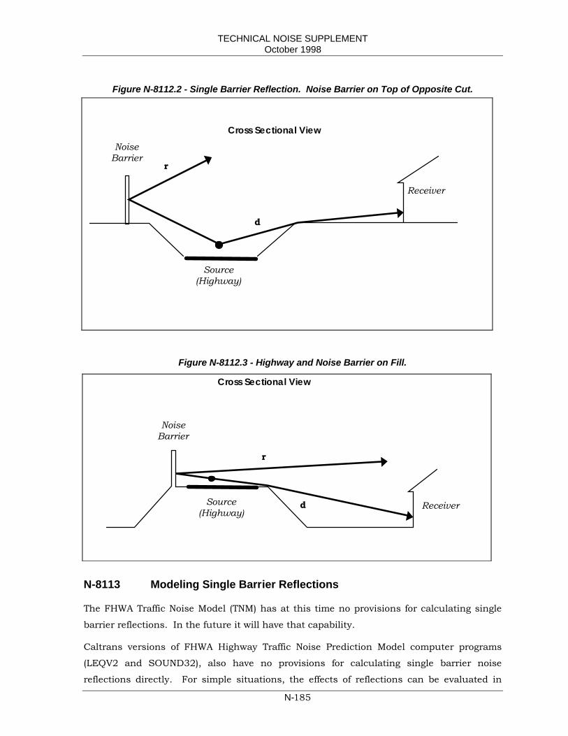
TECHNICAL NOISE SUPPLEMENTOctober 1998
N-185
Figure N-8112.2 - Single Barrier Reflection. Noise Barrier on Top of Opposite Cut.
Figure N-8112.3 - Highway and Noise Barrier on Fill.
N-8113 Modeling Single Barrier Reflections
The FHWA Traffic Noise Model (TNM) has at this time no provisions for calculating single
barrier reflections. In the future it will have that capability.
Caltrans versions of FHWA Highway Traffic Noise Prediction Model computer programs
(LEQV2 and SOUND32), also have no provisions for calculating single barrier noise
reflections directly. For simple situations, the effects of reflections can be evaluated in
Source(Highway)
Receiver
Receiver
Cross Sectional View
Source(Highway)
r
d
NoiseBarrier
NoiseBarrier
Cross Sectional View
d
r
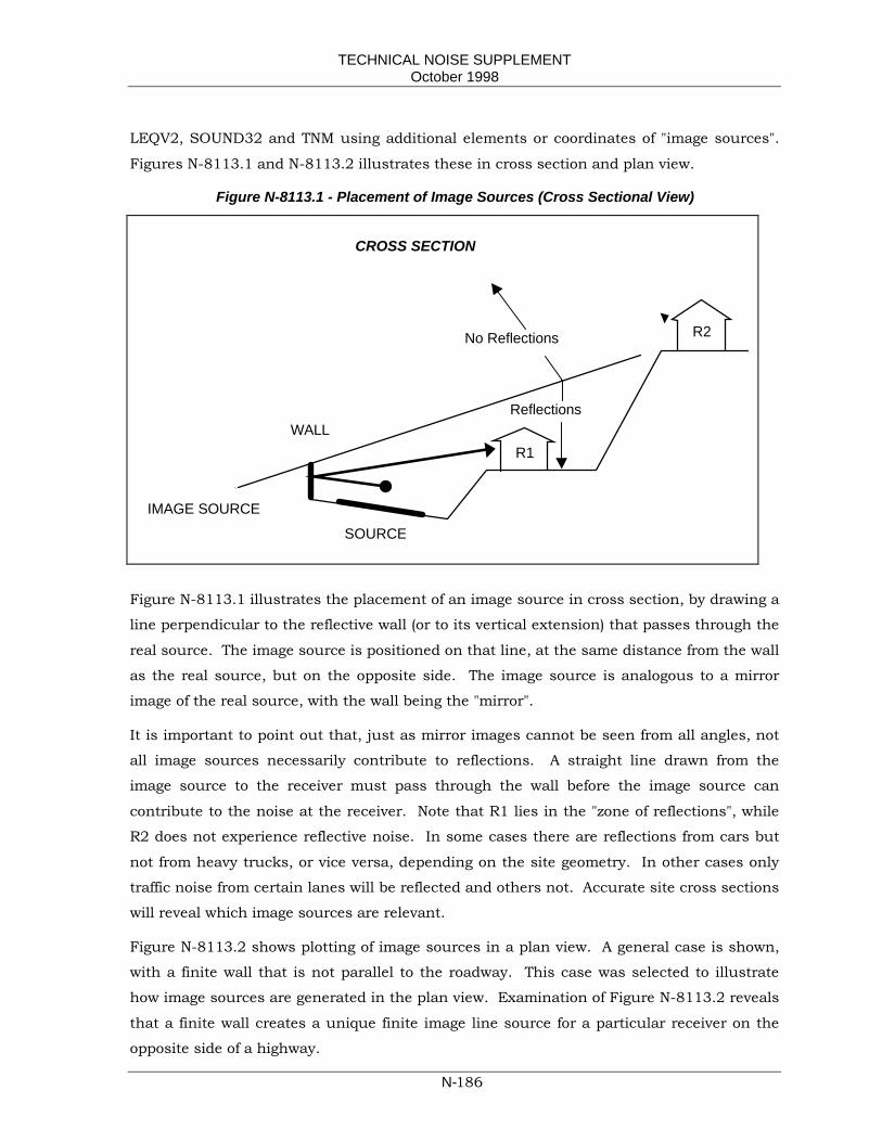
TECHNICAL NOISE SUPPLEMENTOctober 1998
N-186
LEQV2, SOUND32 and TNM using additional elements or coordinates of "image sources".
Figures N-8113.1 and N-8113.2 illustrates these in cross section and plan view.
Figure N-8113.1 - Placement of Image Sources (Cross Sectional View)
Figure N-8113.1 illustrates the placement of an image source in cross section, by drawing a
line perpendicular to the reflective wall (or to its vertical extension) that passes through the
real source. The image source is positioned on that line, at the same distance from the wall
as the real source, but on the opposite side. The image source is analogous to a mirror
image of the real source, with the wall being the "mirror".
It is important to point out that, just as mirror images cannot be seen from all angles, not
all image sources necessarily contribute to reflections. A straight line drawn from the
image source to the receiver must pass through the wall before the image source can
contribute to the noise at the receiver. Note that R1 lies in the "zone of reflections", while
R2 does not experience reflective noise. In some cases there are reflections from cars but
not from heavy trucks, or vice versa, depending on the site geometry. In other cases only
traffic noise from certain lanes will be reflected and others not. Accurate site cross sections
will reveal which image sources are relevant.
Figure N-8113.2 shows plotting of image sources in a plan view. A general case is shown,
with a finite wall that is not parallel to the roadway. This case was selected to illustrate
how image sources are generated in the plan view. Examination of Figure N-8113.2 reveals
that a finite wall creates a unique finite image line source for a particular receiver on the
opposite side of a highway.
IMAGE SOURCE
SOURCE
R1
R2
WALLReflections
No Reflections
CROSS SECTION

TECHNICAL NOISE SUPPLEMENTOctober 1998
N-187
Figure N-8113.2 - Placement of Image Sources (Plan View)
To "construct" the finite image line source, lines perpendicular to the wall (or its extensions)
at two different locations (say P and Q) can be drawn. Along these lines, distances "p" and
"q" from the wall to the roadway line l, at P and Q respectively, can be drawn on the image
side of the wall (p = p' and q = q'). A line l' connecting the two points defined by distances
p' and q' establishes the direction of the image line source. Next, the termini of the infinite
image line source can be determined by the intersections of line l' with two lines from the
receiver R through both end points of the wall. S1' and S2' are now the end points of the
finite image line source.
When using LEQV2 program the wall has to be parallel to the roadway. The above process
can be used for this special case. The finite image line source will then run parallel to the
roadway, and can be defined as an additional element(s), with a segment angle φ. A cross
sectional drawing is needed to reveal if all image traffic (and image roadways) should be
included. If, for instance the heavy trucks do not produce reflections, the heavy truck
volume for the image source can be coded as 0.
Needless to say, only primary reflections should be considered when employing the above
methods. And since each receiver is affected by a different set of reflections, the number of
receivers modeled should be kept to a minimum. Even then, modeling of reflective noise
can be a very cumbersome process. FHWA Traffic Noise Model (TNM), presently being
phased in, does not have, at this time, provisions for reflection calculations other than the
parallel barrier analysis mentioned in the next section. However, it is anticipated that in
P Q
p
p’
q
q’
x2
x’2
x1
x’1
S1
S’1
S2
S’2
Sx
S’x
Infinite Line Source
Finite Image Line Source
Reflective Wall
RPLAN VIEW
l
l’
φ

TECHNICAL NOISE SUPPLEMENTOctober 1998
N-188
the near future single barrier reflections will be included in routine calculations in TNM,
eliminating the need for manipulating the input source data.
N-8120 Parallel Barrier ReflectionsMultiple reflections between reflective parallel noise barriers (noise barriers on each side of
the highway) can potentially reduce the acoustical performance of each individual barrier.
Figure N-8120.1 shows a simple illustration of only five of the many possible reflective
paths in addition to the direct path to the top of the barrier. Theoretically, there are an
infinite number of possible reflective noise paths. Each reflection essentially becomes a
new source, which may add to the noise diffracted by the barrier nearest to the receiver.
This in turn may reduce the barrier's effectiveness.
Figure N-8120.1 clearly shows, however, that as the number of reflections for each possible
path increases, the path length becomes significantly longer. However, in all instances the
barrier to receiver distance is the same. Only that portion of the path length from source to
receiver that lies between the barriers changes. For the direct path this distance is W - S,
where W is the separation distance between the two barriers and S is the distance between
the far barrier to the source. For the first reflective path the distance is approximately (W +
S), and for the second reflective path approximately 3W - S. Further examination of Figure
N-8120.1 shows that the path length difference between the first reflective path and the
direct path is 2S. The difference between the second and first reflective paths is 2(W - S).
The pattern repeats itself for subsequent reflections. These increases in path length
distances for each subsequent reflection soon make their contribution to the total diffracted
noise insignificant, i.e. only the first few reflections are important.
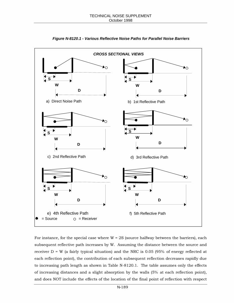
TECHNICAL NOISE SUPPLEMENTOctober 1998
N-189
Figure N-8120.1 - Various Reflective Noise Paths for Parallel Noise Barriers
For instance, for the special case where W = 2S (source halfway between the barriers), each
subsequent reflective path increases by W. Assuming the distance between the source and
receiver D = W (a fairly typical situation) and the NRC is 0.05 (95% of energy reflected at
each reflection point), the contribution of each subsequent reflection decreases rapidly due
to increasing path length as shown in Table N-8120.1. The table assumes only the effects
of increasing distances and a slight absorption by the walls (5% at each reflection point),
and does NOT include the effects of the location of the final point of reflection with respect
WS
DW
S
D
WS
D
WS
D
WS
DW
S
D
a) Direct Noise Path b) 1st Reflective Path
c) 2nd Reflective Path d) 3rd Reflective Path
e) 4th Reflective Path f) 5th Reflective Path
CROSS SECTIONAL VIEWS
= Source = Receiver

TECHNICAL NOISE SUPPLEMENTOctober 1998
N-190
to the source location. This affects the amount of diffraction by the wall on the receiver
side, which will be different for each of the reflective paths. Also ignored are pavement
reflections, constructive and destructive interference of the sound waves, frequency shifts
and the effects of the traffic mix, traffic stream, and lane distribution.
Table N-8120.1 - Contribution of Reflections for the Special Case where W=2S, D=W, and NRC=0.05.
NOISE PATH DISTANCE,(RE: W)
(Source toReceiver)
DISTANCEADJUSTMENT,(
Direct toReflective Path)
10Log(W/XW)(X=2,3, ,11)
dBA(1)
ABSORBED,(NRC=0.05),
dBA
(2)
CONTRIBUTION,(RE: Direct),
dBA
(1+2)
CUMULATIVETOTAL NOISE
LEVEL(RE: Direct),
dBA(Direct +
1st Refl. + 2ndRefl., etc.)
Direct W 0 (Ref.) 0 0 (Ref.) 0 (Ref.)
1st Reflective 2W -3.0 -0.2 -3.2 +1.7
2nd Reflective 3W -4.8 -0.45 -5.25 +2.5
3rd Reflective 4W -6.0 -0.7 -6.7 +3.0
4th Reflective 5W -7.0 -0.9 -7.9 +3.3
5th Reflective 6W -7.8 -1.1 -8.9 +3.6
6th Reflective 7W -8.5 -1.3 -9.8 +3.8
7th Reflective 8W -9.0 -1.6 -10.6 +3.9
8th Reflective 9W -9.5 -1.8 -11.3 +4.1
9th Reflective 10W -10.0 -2.0 -12.0 +4.2
10th Reflective 11W -10.4 -2.2 -12.6 +4.3
Noise contributions from parallel barrier reflections are obviously depended on the source
to receiver distance. For a fixed W, the relative distance attenuation for each reflective path
decreases as the D increases. The contribution of each reflection also increases as W
decreases in relation to D (Figure N-8120.1).
Noise contributions of reflections between parallel barrier degrade the performance
(insertion loss) of each noise barrier. How much degradation takes place depends of course
on the site geometry and barrier configurations. In addition to the factors shown in Figure
N-8120.1 and Table N-8120.1, there is another important relationship between the ratio of
the separation between two parallel barriers (W) and their average height (HAVG), and the
amount of insertion loss degradation. As a rule, if the W/HAVG ratio is 10:1 or greater, the
insertion loss degradation is less than 3 dBA, and not noticeable to the human ear. This
has been supported by Caltrans research and research done by others. Because of noise

TECHNICAL NOISE SUPPLEMENTOctober 1998
N-191
barrier height restrictions of 5 m (16 ft), parallel noise barriers in California have a W/H of
10:1 or greater. Although there have been claims to this effect, there are no known
instances where reflective parallel noise barriers in any configuration, anywhere, have ever
measurably increased noise levels over those without noise barriers. The W/HAVG guideline
applies not only to noise barriers but also to retaining walls or combinations of both.
Figure N-8120.2 shows these concepts.
Figure N-8120.2 - W/HAVG
Ratio Should be 10:1 or Greater
N-8130 REFLECTIONS OFF STRUCTURES AND CANYONEFFECTS
Generally, the same rules that apply to reflections off noise barriers apply to those off
retaining walls. Since the height limitations to noise barriers do not pertain to retaining
walls, there is a greater potential for noise reflections, especially when the retaining walls
are along stretches of depressed freeways. However, no noise barriers in this configuration
have ever been shown objectively and conclusively to result in higher noise levels than
those of a similar, at-grade freeway because of reflective noise.
Complex multi-level highway interchanges can present some challenging problems in noise
abatement design. The widespread spatial distributions of traffic noise sources and
receivers make it difficult to design noise barriers that interrupt all direct noise paths
between the many source-to-receiver combinations. Additionally, reflective surfaces of
concrete structural components create many opportunities for noise reflections to
HAVG
W
W
HAVG
ROADWAY
ROADWAY
NOISE BARRIERS
RETAINING WALLS
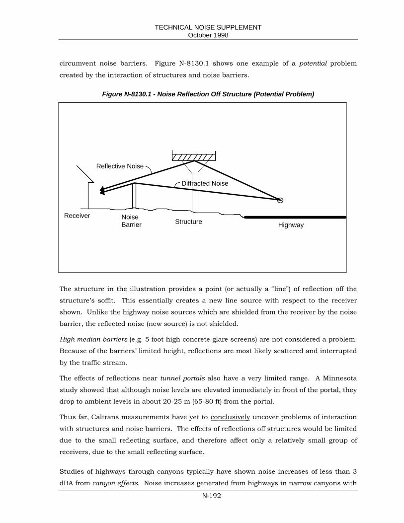
TECHNICAL NOISE SUPPLEMENTOctober 1998
N-192
circumvent noise barriers. Figure N-8130.1 shows one example of a potential problem
created by the interaction of structures and noise barriers.
Figure N-8130.1 - Noise Reflection Off Structure (Potential Problem)
The structure in the illustration provides a point (or actually a “line”) of reflection off the
structure’s soffit. This essentially creates a new line source with respect to the receiver
shown. Unlike the highway noise sources which are shielded from the receiver by the noise
barrier, the reflected noise (new source) is not shielded.
High median barriers (e.g. 5 foot high concrete glare screens) are not considered a problem.
Because of the barriers’ limited height, reflections are most likely scattered and interrupted
by the traffic stream.
The effects of reflections near tunnel portals also have a very limited range. A Minnesota
study showed that although noise levels are elevated immediately in front of the portal, they
drop to ambient levels in about 20-25 m (65-80 ft) from the portal.
Thus far, Caltrans measurements have yet to conclusively uncover problems of interaction
with structures and noise barriers. The effects of reflections off structures would be limited
due to the small reflecting surface, and therefore affect only a relatively small group of
receivers, due to the small reflecting surface.
Studies of highways through canyons typically have shown noise increases of less than 3
dBA from canyon effects. Noise increases generated from highways in narrow canyons with
HighwayReceiver Noise
Barrier Structure
Reflective Noise
Diffracted Noise

TECHNICAL NOISE SUPPLEMENTOctober 1998
N-193
steep side slopes theoretically could be greater than 3 dBA, depending on ground cover and
the steepness and smoothness of side slopes. The canyon walls, to some extent, act as
parallel sound walls with respect to multiple reflections. However, unless the slopes are
perfectly vertical, build up of reflections will be more limited due to the slope angles.
Highways on hill sides with near vertical rock cuts are somewhat similar to the single
barrier situation discussed before. No perceptible noise increases are expected. Due to the
angle of the cut slope, reflections are directed skyward, while receivers would most likely be
below the highway.
N-8140 MINIMIZING REFLECTIONS
When designing reflective parallel noise barriers it is recommended that a minimum 10:1.
W/HAVG is maintained between the two barriers, in order to avoid the possibility of
perceivable barrier performance degradations. Earth berm noise barriers are not reflective
and are therefore not affected by W/HAVG ratios of less than 10:1.
Sound absorption has been promoted as a solution for noise reflection where actual
problems would be identified. As part of an on-going program Caltrans considers a variety
of proprietary noise barrier products and systems, some of which have sound absorptive
characteristics. For reasons of structural integrity, safety, cost, or other factors, no
absorptive material has been approved yet. For more information on barrier materials and
new products, the designer should check with HQ Design and Local Programs for
availability of approved materials, and the Office of Structures Design to determine which
materials have been approved for use on noise barriers. Sound-absorptive materials can
either be an inherent property of the barrier, or it can be added on to an existing barrier
(retrofit). Either way, the cost of the barrier will likely increase substantially.
The amount of noise absorption of the materials is rated by a noise absorption coefficient α.
The coefficient is defined as the ratio of the acoustical energy absorbed by the material to
the total energy incident upon that material. For any particular material, α is frequency-
dependent, and its value for each specific frequency ranges from 0 (perfect reflector) to 1
(perfect absorber). In order to rate the overall absorptive characteristics of the material, a
measure of the average α over the frequency range of interest is useful. For traffic noise
frequencies, an appropriate measure is the Noise Reduction Coefficient (NRC), which is the
arithmetic average of a in four octave bands with center frequencies of 250, 500, 1000, and
2000 Hz, calculated by:
NRC =(α250 + α500 + α1000 + α2000)/4

TECHNICAL NOISE SUPPLEMENTOctober 1998
N-194
If approved absorptive materials are considered, a minimum NRC of 0.85 should be used as
a criterion. This value means that 85% of the incident noise energy is absorbed and only
15% reflected. For a single reflection this can only add a maximum of 0.6 dBA to the direct
noise level, instead of the theoretical 3 dBA for a perfect reflector (NRC = 0).
N-8200 EFFECTS OF NOISE BARRIERS ON DISTANTRECEIVERS
N-8210 BACKGROUND
With the proliferation of noise barriers in California, some recent public concern has
emerged that under certain conditions of topography and meteorology noise barriers
increase noise levels at receivers between 1/2 km to 3 km (more than 1/4 mile to 2 miles)
from freeways. The concerns are based on subjective perception only. No objective
evidence based on noise measurements has ever been advanced that noise barriers
increase noise levels at any distance, other than under the limited conditions described in
section N-8100.
The concerns raised by various homeowner groups in the San Francisco Bay Area and the
Los Angeles Area include all three possible categories of source/ barrier/ receiver
configurations:
1. Reflective noise barriers on the sides of highways opposite from that of the receivers
(i.e. highways between barriers and receivers)
2. Parallel reflective noise barriers on each side of highways
3. Noise barriers between highways and receivers
The first two issues involve reflective noise of single and parallel barriers, discussed in
previous section N-8100. The third issue, however, deals with diffracted noise. All of the
issues involve long noise propagation distances, which are difficult to study due to the
numerous variables in topography and meteorology. Caltrans experience has been that
atmospheric conditions can fluctuate noise levels at those distances by more than 10 dBA,
with or without noise barriers.
Refraction is the principle atmospheric process responsible for the fluctuations. A vertical
gradient of either temperature or wind velocity produces a corresponding vertical gradient
of sound velocity. This causes sound waves to refract (bend) either upwards or downwards.
Upward refraction occurs during sound propagation in upwind direction or normal
temperature lapse conditions (air temperatures decreasing with height). This tends to send
TECHNICAL NOISE SUPPLEMENTOctober 1998
N-195
noise skyward, leaving a noise “shadow” near the ground and thereby reducing noise levels.
This occurs with or without noise barriers. Downward refraction occurs during sound
propagation in downwind direction, or in temperature inversions (temperature increasing
with height above the ground). Downward refraction tends to send skyward noise down,
concentrating noise near the ground, thereby increasing noise levels, both with and without
a barrier. Atmospheric refraction of sound waves was discussed in section N-2143.
N-8220 COMPLETED STUDIES
N-8221 Caltrans Reflective Noise Studies
On the issue of reflective noise, Caltrans has done two very detailed studies, one along 07-
LA-405 in the Los Angeles community of Brentwood, and another along 03-Sac-99 in south
Sacramento. These studies dealt with the acoustical performance of parallel noise barriers
and the possibility of noise reflection problems. The studies are described in the following
reports:
1. Hendriks, R., J.Hecker, “Parallel Noise Barrier Report: A Noise Absorptive
Demonstration Project - San Diego Freeway, Interstate Route 405 in the City of Los
Angeles, Community of Brentwood”, California Department of Transportation,
District 7 Environmental Investigations Section (With Assistance of Transportation
Laboratory), Los Angeles, CA., July 1989.
2. Hendriks, R., “Field Evaluation of Acoustical Performance of Parallel Noise Barriers
Along Route 99 in Sacramento, California”, Report No. FHWA/CA/TL-91/01,
California Department of Transportation, Division of New Technology, Materials and
Research, Sacramento, CA., January 1991.
The L.A. study (1) was part of a demonstration project to test acoustically absorptive
treatment on one of two parallel masonry sound walls. The project was initiated by District
7 (Los Angeles) in response to concerned home owners living in Brentwood at distances of
0.3 - 0.6 km (0.2 to 0.4 miles) away from the freeway. The terrain between the residences
and the freeway ranged in height from -6 to +15m (-20 to +50 ft) relative to the freeway and
was occupied by single and multi-story residential units. Some homeowners perceived an
increase in noise when the opposite sound wall was constructed about seven years after the
near sound wall had been completed. Legal action was initiated to have Caltrans remove
the wall or have it treated with a noise absorptive material. No noise level increase had
been perceived when the first (near) barrier was constructed.

TECHNICAL NOISE SUPPLEMENTOctober 1998
N-196
In 1987 the Division of New Technology, Materials and Research (NT,M&R), also known as
TransLab - was contacted to perform the before and after treatment noise study. NT,M&R’s
approach was to take simultaneous noise measurements at 14 different locations, of which
11 were in the vicinity of the freeway sound walls, at distances up to 61 m (200 ft) from the
near wall and at heights of up to 7m (23 ft) above the ground, and the remaining 3 near the
residences. Concurrent meteorological observations (wind speed, direction, temperature
and humidity) and lane-by-lane traffic counts on the Route 405 freeway, on/off ramps, and
Sunset Boulevard were also taken. Fifteen “before” and ten “after” measurements were
taken at the freeway sites; twenty-seven before and twenty-two after at the 3 distant sites.
Each measurement lasted 15 minutes. About thirty District 7 and NT,M&R personnel
participated in the study. At Caltrans’ request an expert in the discipline of transportation
noise, Dr. William Bowlby from Vanderbilt University, also participated in the study by
analyzing the data independently. His results and method of analysis were reported the
following document:
3. Bowlby, W., “Parallel Noise Barrier Study, 07-LN-405, Prediction and Analysis of
Data Before and After Acoustical Treatment”, Submitted to California Department of
Transportation, District 7, Los Angeles, CA, Contract 07D527, Department of Civil
and Environmental Engineering, Vanderbilt University, Nashville, Tennessee, June
2, 1989.
The before and after data were carefully matched by wind speed and direction, and
normalized for traffic variations.
Analyses in (1) and (3) showed that the acoustical material reduced the noise by an average
of 1 dBA. Human ears cannot perceive a change of 1 dBA. Since the acoustic material was
an almost perfect noise absorber of the reflective noise, the after treatment condition, in
essence, simulated a no wall condition on the opposite side of the freeway. From the
results NT,M&R concluded that there was no reflection problem to begin with.
However, fluctuations in noise levels at 0.3 km (0.2 miles) and greater were as large as 8
dBA with relatively minor changes in wind speed and direction. Even at 61 m (200 ft)
behind the barrier minor wind shifts were responsible for noise fluctuations of about 4 dBA.
Wind was the single most important factor in changing noise levels at distances beyond 61
m (200 ft) from the barrier, even greater than differences in traffic volumes.
In 1991 NT,M&R completed the Sac-99 study (2), which represented one of the first
systematic attempts to quantify the effects of multiple reflections between parallel masonry
sound walls for configurations representative of many barrier locations in California. The

TECHNICAL NOISE SUPPLEMENTOctober 1998
N-197
research consisted of extensive noise, traffic, and meteorological measurements and
analyses during three stages: 1) without any sound walls, 2) after construction of the near
sound wall, and 3) after completion of the far sound wall. More than one-hundred 15-
minute measurements were taken at 11 locations, simultaneously, ranging from 0 to 61 m
(200 ft) behind the near barrier and at heights of 1.5 to 7 m (5 to 23 ft) above the ground.
The objective was to determine how much the performance of the near barrier would be
decreased by the reflections off the far barrier. Once again, the staged data were carefully
matched by meteorology. The results indicated that the average reduction in near sound
wall performance ranged from 0 to 1.4 dBA, well below the generally recognized 3 dBA
human perception threshold of changes in noise levels. As was the case with the L.A.
study, the data showed large fluctuations in noise that occurred during all three stages (i.e.
with or without noise barriers) as a result of meteorological conditions. Under all measured
conditions, however, the barrier provided adequate insertion loss.
The above studies were performed under carefully documented “real world” conditions and
showed no evidence of reflection problems. However, the studies did clearly demonstrate
the profound effect of meteorological conditions on traffic noise levels. Any before and after
comparisons of noise data should therefore be matched as carefully as possible by
meteorological conditions to be meaningful. Given the number of variables involved, the
level of effort and cost that must go into a noise study involving long distances is
substantial.
N-8222 Reflective Noise Studies by Others
The U.S. Department of Transportation, Volpe National Transportation Systems Center
completed two parallel barrier studies during the period of October 1986 through April
1994. The studies were funded by the highway agencies of seventeen states, including
Caltrans. The findings of the two studies are reported in:
4. Fleming, G.G., E. Rickley, “Performance Evaluation of Experimental Highway Barriers”,
Report Number DOT-VNTSC-FHWA-94-16, U.S. Department of Transportation,
Research and Special Programs Administration, John A. Volpe National Transportation
Systems Center, Cambridge, MA 02142, April 1994.
The first study examined the performance of two parallel experimental highway noise
barriers constructed on opposite sides of a two-lane asphalt service road at Dulles
International Airport near Washington, D.C. The barriers were constructed in such a way
that they could be configured to have absorptive and/or reflective roadside facades, or be
independently tilted outward, away from the roadway, at angles of 7, 15, and 90 degrees. A

TECHNICAL NOISE SUPPLEMENTOctober 1998
N-198
90-degree tilt angle simulated effective removal of the barrrier. The barrier behind which
noise measurements were made was 152 m (500 ft) in length; the barrier on the opposite
side was 76 m (250 ft) long and centered on the 152 m barrier. For each of 12 individual
barrier configurations, noise and meteorological measurements were made at 10 locations
behind the 152 m barrier and 10 locations in an adjacent open field site, using the same
distances from the noise sources and heights above the ground. The noise sources were
four individual test trucks and an artificial fixed point source (speaker system) used to
simulate a pass by of each test truck.
The Dulles site was not representative of the typical parallel barrier sites along California
highways. Although the 4.3 m height of the barriers was typical, the 26 m (86 ft)
separation (width) between the two barriers was much narrower than typical highway
widths. This translates into a width/height (w/h) ratio of 6:1 for the Dulles barriers, while
almost all parallel barrier sites in the U.S. have at least a 10:1 ratio. The Dulles study
concluded that the worst insertion loss degradation reached as high as 6 dBA due to
multiple reflections between the parallel reflective barrier facades.
A second site along I-495 in Montgomery County, Maryland, was used to measure parallel
barrier degradation under more realistic yet still severe conditions of free-flowing traffic but
a w/h ratio of 9:1 (still less than typical). The degradations were measured using 10
microphone locations behind a parallel barrier section and simultaneously at 10 locations
behind a single wall adjacent to the parallel barriers. In this configuration the maximum
degradation reached 2.8 dBA.
Together with the Caltrans studies (1 and 2) the report (4) concluded that parallel barrier
sites with w/h ratios of 10 or more would have a degradation of less than 3 dBA, an
imperceptible noise increase over a single barrier.
N-8223 Noise Levels Behind A Single Noise Barrier
The third issue, that of perceived increases in noise levels behind a single noise barrier on
the same side of a freeway, relates in part to the above mentioned studies. The noise level
fluctuations at distant receivers are far more influenced by varying meteorological
conditions than the presence or lack of a noise barrier. Therefore, any study designed to
examine with and without barrier conditions will certainly have to include detailed
meteorological documentation. Atmospheric equivalency must first be established, before
any comparisons of before and after barrier noise data should be made.
There is no question that noise barriers are effective in the vicinity of highways, say within
100 m (330 ft). Caltrans has collected enough data over the years to substantiate this. The

TECHNICAL NOISE SUPPLEMENTOctober 1998
N-199
following report compared before and after noise measurements at eleven noise barrier sites
with those predicted by noise barrier acoustical design procedures:
5. Hendriks, R.W., “Evaluation of Noise Barriers”, Report No. FHWA/CA/TL-81/07,
California Department of Transportation, Office of Transportation Laboratory,
Sacramento, California, June 1981.
The measurements were part of an overall evaluation of noise barriers’ performances, noise
barrier acoustical design procedures, and community acceptance.
Caltrans has also experienced, in the course of many measurements, that beyond 100 m or
so, noise levels often approach ambient levels (the noise levels associated with normal day-
to-day activities in the community). For obvious reasons, a sound wall cannot attenuate
noise below these levels. However, Caltrans has never experienced noise increases (over
no-barrier noise levels) at any distance behind noise barriers. Yet, some persist that noise
barriers will increase noise levels at distant receivers.
Explanations have sometimes centered on noise waves “going over the wall and coming
back to the ground”. This is “diffraction” and is actually responsible for noise attenuation,
rather than an increase in noise, when compared with the direct noise received without a
noise barrier. (See sections N-2144, N-4510, and N-6100).
Another popular “explanation” for perceived increase in noise due to sound walls is that the
sound wall “lifts” the noise over tiers of homes that normally would shield the receiver. Yet,
a sound wall will no more elevate the noise source over tiers of homes than the intervening
homes will. Sound walls in California are generally restricted in height to 16 feet, an
amount approximately equal to the average height of residential development.
There is, however, a loss of “ground effect” behind a noise barrier (see sections N-4520 and
N-6131). Without a noise barrier the direct path of the traffic noise to the receiver travels
closer to the ground than after a noise barrier is built. Noise waves close to the ground are
subject to excess attenuation due to absorption by the ground. Therefore, when a noise
barrier is built there is a trade-off between barrier attenuation (a decrease in noise) and a
loss of excess attenuation.
The net reduction of noise due to the barrier attenuation and loss of excess attenuation is
called “barrier insertion loss”(Section N-6131). Close to a barrier, there is no question that
the barrier attenuation benefit far outweighs the loss of excess attenuation. At further
distances, however, barrier attenuation diminishes while the cumulative effects of the loss
of excess attenuation increase. Our acoustical design procedures for noise barriers take
these factors into consideration by applying different noise drop-off rates to with and

TECHNICAL NOISE SUPPLEMENTOctober 1998
N-200
without noise barrier cases. If we were to keep these drop-off rates constant and apply
them to long distances, there would indeed be a distance at which the loss in ground effect
would eventually exceed the barrier attenuation.
Extensive amounts of field data gathered during a Caltrans noise propagation research
project shows that differences between excess attenuation rates of elevated sources (e.g.
truck stacks, noise diffracted over a noise barrier) and those close to the ground (e.g. tire
noise) diminish after a hundred meters (few hundred feet) or so. The findings can be
applied to noise barriers which in essence “elevate” the source. The cumulative effect of
decreasing differences in elevated and near-ground excess attenuation rates with distance
appear to cause a “bulge” at about 60 - 90 m (200 - 300 ft) behind the barrier where the
effect of the differences is the greatest. At greater distances the differences in elevated and
near-ground noise levels appear to become smaller again until they disappear at some
distance beyond 120m (400 ft). The research was documented in the following report:
6. Hendriks, R.W., “Traffic Noise Attenuation as a Function of Ground and Vegetation
(Final Report)”, Report No. FHWA/CA/TL-95/23, California Department of
Transportation, Engineering Service Center, Office of Materials Engineering and Testing
Services, Testing and Technology Services Branch, Sacramento, CA, June 1995.
Questions have also been raised at times about whether noise “redirected” by noise barriers
“bounces off” temperature inversion layers. Although NT,M&R did not have
instrumentation to measure inversion layers in the L.A. study, the probability of the
presence of one was very high during the early morning measurements under calm
conditions. At any rate, “redirections” on the scale being discussed, involves a maximum of
5m (16 ft) high noise barriers and a distance of 400 m (1/4 mile) or more, are less than one
degree and therefore negligible.
In July 1994, Caltrans contracted with a consulting firm to do a detailed before and after
noise barrier study along I-680 near Walnut Creek. Caltrans had previously received
complaints from residents in nearby Danville who claimed that recently constructed noise
barriers increased noise levels more than 0.4 km (1/4 mile) from the freeway. The study
was part of an on-going effort by Caltrans to find out if noise barriers do indeed increase
noise levels at some distance from a freeway. The study concentrated on receivers from 0.4
to 1 km (1/4 to 2/3 mile) behind a 3.6 m (12 ft) high noise barrier, 1.2 km (3/4 mile) long.
The study included before and after noise barrier noise measurements of traffic noise,
traffic volumes and speeds, traffic mix, and meteorological conditions. All before and after
noise measurements were carefully matched by meteorology and normalized for different

TECHNICAL NOISE SUPPLEMENTOctober 1998
N-201
traffic conditions. Although the noise barrier actually decreased noise levels the amounts
were insignificant and the conclusion was that the noise barrier did not affect the noise
levels at the distant receivers. The results and methodology of the study are described in:
7. “Interstate 680 Livorna - Stonecastle Soundwall Study”, Woodward-Clyde Consultants,
Oakland, California, and Illingworth and Rodkin, Inc., Fairfax, California, Submitted to
California Department of Transportation, Oakland, California, July 1994.
The study also included measurements on the opposite side of the freeway to measure
reflections off the noise barrier. As expected, there was a noise level increase of 0-2.4 dBA,
with an average of 1.5 dBA. Such a small increase is not noticeable by the human ear.
After years of research, Caltrans has found no objective evidence that noise levels increase
perceptibly due to noise barriers. It is widely accepted by acousticians that changes in
traffic noise levels need to be 3 dBA before they can be perceived by human ears. Such
increases in noise levels due to noise barriers have never been measured.
N-8230 STUDYING THE EFFECTS OF NOISE BARRIERS ONDISTANT RECEIVERS
Allegations of noise barriers increasing noise levels at distant receivers based on perception
only are at best unreliable. With possible noise fluctuations of more than 10 dBA due to
meteorological factors alone, person(s) making such claims must remember not only the
before barrier noise levels, but also have knowledge of the meteorological conditions
associated with those noise levels. In order to confirm whether noise barriers indeed do
increase noise levels in some instances, a complex before and after barrier field study must
be undertaken.
Before and after noise barrier(s) noise measurements do not adequately address the
previous issues unless the measurements are carefully matched by before and after
conditions of meteorology, traffic, and topography. Such studies are not at this time
considered routine. Technical Advisory TAN-97-01-R9301 “General Guidelines for the
Effects of Noise Barriers on Distant Receivers”, issued in 1997, gives guidelines and criteria
to cover these studies. This Technical Advisory can be obtained from the Caltrans
Environmental Program, Environmental Engineering – Noise, Air Quality,, and Hazardous
Waste Management Office, in Sacramento, CA.
TECHNICAL NOISE SUPPLEMENTOctober 1998
N-202
N-8300 STOP AND GO TRAFFICSection N-5510 covered the California version of the FHWA traffic noise prediction model
per FHWA-RD-77-108. The computer programs SOUND32 and LEQV2 predict the hourly
Leq for constant-speed traffic. The model is not equipped to deal with “stop and go” driving
conditions typical of ramps, arterials and city streets.
A model suitable for use with STAMINA 2.0 (Federal computerized version of the FHWA
Model) has been developed by Dr. William Bowlby of Vanderbilt University under contract
to the National Cooperative Highway Research Program (NCHRP). The former Division of
New Technology Transportation Materials and Research further revised this model for use
with SOUND32 (California version of the STAMINA 2.0). The full report in which the model
and its use with STAMINA 2.0 is described is:
8. Bowlby, W., R.L.Wayson, and R.E. Stammer, Jr., “Predicting Stop-and-Go Traffic Noise
Levels”, NCHRP Report 311, Transportation Research Board, National Research
Council, Washington, D.C., November 1989.
The report, excerpts from the report, and revisions for use with SOUND32 are available
from Caltrans Environmental Program, Environmental Engineering – Noise, Air Quality,
and Hazardous Waste Management Office, in Sacramento, CA.
When TNM (see Section N-5520) is mandated, the above method will be obsolete. TNM has
provisions for dealing with interrupted-flow traffic.

TECHNICAL NOISE SUPPLEMENTOctober 1998
N-203

TECHNICAL NOISE SUPPLEMENTOctober 1998
N-203
N-9000 GLOSSARY
The terms and definitions in this glossary are either used in this Supplement, or are
commonly found in environmental noise literature. To make this glossary more useful to
the highway traffic noise analyst, the definitions herein are generally biased towards
highway traffic noise and the abatement thereof, instead of general acoustics.
Absorption (of Sound) - The attenuation of sound (noise) caused by conversion of soundenergy into other forms of energy (usually heat) within a medium. Absorption is a propertyof the medium (material). In noise barrier material, absorption can be thought of as thecomplement of reflection. A perfectly absorptive material does not reflect any sound energy;a non-absorptive (reflective) material reflects almost all of the sound energy. In either case,a small portion of sound energy is transmitted through the barrier and continues inroughly the same direction as the incident noise propagation. (See Transmission Loss). Intypical highway traffic noise barriers, the sound energy passing through is less than 1% ofthe incident noise energy.
Absorption Coefficient - A term that approximately equals the ratio of sound energyabsorbed by a material to the energy incident upon the material. Absorption coefficientsrange from 0 (no absorption) to 1 (perfect absorption). In highway noise barriers, materialwith an absorption coefficient of 0 will reflect back almost all the incident noise energy;material with a coefficient of 1 will not reflect back any sound energy. The absorptioncoefficient is dependent on material, the sound frequency and angle of incidence.
Absorptive Grounds - Types of ground (such as normal earth and most grounds withvegetation) that are absorptive to sound energy, and that reverse the phase of reflectedenergy at grazing angles of incidence. (See also soft sites and ground effects).
Acoustics - The broad field of science that deals with the production, propagation, reception,effects, and control of sound, audible and inaudible to the human ear, and occurring in allmedia.
Airborne Sound - Sound that reaches the point of interest primarily by propagation throughthe air.
Ambient Noise (Level) - All-encompassing noise (level) at a given place and time, usually acomposite of sounds from all sources near and far, including any specific source(s) ofinterest.
Amplitude - The strength or magnitude of the pressure of a sound wave.
Anechoic Chamber (Room) - A room whose boundaries have been designed to absorb nearlyall of the sound incident on them, thereby affording a test room essentially free fromreflected sound, simulating a free field conditions for the limited space defined by theroom’s boundaries.
Angle of Diffraction - The angle through which sound energy is diffracted (bent) as it passesover the top of a noise barrier and then proceeds towards the receiver. Receivers deeperinto the shadow zone have larger angles of diffraction, and therefore greater barrierattenuation. (See Diffraction, Shadow Zone.)
TECHNICAL NOISE SUPPLEMENTOctober 1998
N-204
Angle of Incidence - The angle formed by the radial line of sound waves striking a surface ata specific location and the plane of that surface. (See angle of reflection).
Angle of Reflection - The angle formed by the radial line of sound waves reflecting off asurface at a specific location and the plane of that surface. (See angle of incidence).
Atmospheric Effects - Sound absorption by air molecules and water vapor, sound refractioncaused by temperature and near-ground wind gradients, and air turbulence are collectivelycalled atmospheric effects. Although atmospheric effects are mostly responsible forsubstantial noise fluctuations at distant receivers, they also can have a significant effect atdistances within a 100 m (330 feet).
Audible (Frequency) Spectrum - The frequency range normally associated with humanhearing, usually considered between 16 - 20,000 Hz. For noise control purposes, theaudible spectrum of interest usually lies between 20 - 10,000 Hz.
Audiogram - A graph showing hearing loss as a function of frequency.
Audiometer - An instrument for measuring hearing sensitivity or hearing loss.
Automobile - A vehicle classification for the purpose of noise prediction modeling, defined asall vehicles with two axles and four wheels designed primarily for transportation of nine orfewer passengers (automobiles), or transportation of cargo (light trucks). Generally thegross weight is less than 10,000 lbs (4,500 kg).
Average (Noise) Level - Typically the “energy-averaged” noise level in dB, wherein thecontributing levels are first converted to “relative energies” or “energy ratios”, and addedand divided by the number of contributing levels. The result is then converted back to dB.
A-Weighted Sound Level (abbreviated dBA or dB(A)) - Frequency weighted Sound PressureLevel approximating the frequency response of the human ear. It is defined as the soundlevel, in decibels, measured with a sound level meter having the metering characteristicsand a frequency weighting specified in the American National Standards InstituteSpecification for Sound Level Meters, ANSI S 1.4 - 1983. The A-weighting de-emphasizeslower frequency sound sounds below 1000 Hz (1kHz) and higher frequency sounds above 4kHz. It emphasizes sounds between 1kHz and 4 kHz. A-weighting is the most generallyused measure for traffic and environmental noise throughout the world.
Background Noise - The total of all noise in a system or situation, independent of thepresence of the noise source of interest (i.e without the noise of interest).
Baffle - A shielding structure or series of partitions used to increase the effective externaltransmission path length between two points in an acoustic system.
Band - (See Frequency Band)
Band Center Frequency - The designated (geometric) mean frequency of a band of noise.
Band Pressure Level - The sound pressure level contained within a specified band.
(Noise ) Barrier Attenuation - The noise reduction due to barrier diffraction only.
Broadband Noise - Noise with components over a wide range of frequencies.
TECHNICAL NOISE SUPPLEMENTOctober 1998
N-205
Calibrator - A device used to calibrate -or properly adjust for valid measurement results- asound level meter and microphone system. Calibration must be performed before and aftersound level measurement sequence.
Community Noise Equivalent Level (CNEL) - A noise level that takes into account all the A-weighted noise energy from a source during 24 hours and weights the evening (7 to 10p.m.) noise by adding 5 dBA, and night (10 p.m. to 7 a.m.) noise by adding 10 dBA,respectively, during these periods.
Compression (of Sound Wave) - The portion of a sound wave in which the air molecules areslightly compressed with respect to the barometric air pressure (opposite of rarefaction).
Cylindrical Divergence ( - Spreading) - Sound waves generated by a line source, such asapproximated by a highway, tend to form cylindrical wave fronts that propagate byradiating outward from their original line source in cylindrical pressure waves of everincreasing areas. This process is referred to as cylindrical divergence or spreading. Thesame sound energy distributed over an ever increasing cylindrical area is reponsible ofreducing the sound’s energy per unit area (intensity) by one half for each doubling ofdistance. This corresponds with a noise level decrease of 3 dB per doubling of distance.
Cycles Per Second - (See Hertz)
Day-Night Level - (See Ldn)
Decibel (Abbreviated dB) - A decibel is one-tenth of a Bel. It is a measure on a logarithmicscale which indicates the squared ratio of sound pressure to a reference sound pressure(unit for sound pressure level), or the ratio of sound power to a reference sound power (unitfor sound power level). (See sound pressure level, and sound power level).
(Noise) Descriptor - A generic term for a noise indicator such as Leq, Lmax, Ldn, etc.
Diffuse Sound Field - A sound field in which the time average of the mean-square soundpressure is everywhere the same and the flow of acoustic energy in all directions is equallyprobable. For example, a sound source in a reverberation room, where many reflectedsound waves are present and the sound level is equal at any location in the room.
Diffraction - The bending of sound pressure waves around an obstacle. The ease with whichthe pressure waves diffract around an obstacle depends on the ratio of wavelength to thesize of the obstacle. Pressure waves with a given wavelength diffract more readily around asmall object than a large object. Pressure waves with a longer wavelengths diffract moreeasily around an object of a given size than pressure waves with a shorter wavelength. Dueto the above principles, highway traffic noise barriers provide a more defined noise“shadow” behind the barrier (and more noise attenuation) for higher frequency noise thanfor lower frequency noise. (See Angle of Diffraction, Shadow Zone)
Doppler Effect - The change in observed frequency of a sound wave caused by a time rate ofchange in the effective path length between sound source and receiver. If the path lengthrate of change causes the source and receiver to approach each other, the observedfrequency shifts upward. If the source and receiver recede relative to each other, thefrequency shifts downward. The frequency shift is called the Doppler Shift, and the unit isHertz.
Dosimeter - An instrument measuring noise exposure for compliance with OSHA standards.
TECHNICAL NOISE SUPPLEMENTOctober 1998
N-206
Dynamic Range - The range in sound levels (in dB) through which a source or receiver canemit or receive sound. For example, the dynamic range of a sound level meter typicallyranges from 20 - 140 dB.
Emission Level - A measure of the noise output of a single vehicle. It is the maximum noiselevel, in dBA, observed during a passby of the vehicle at 15 m (50 ft). (See also ReferenceEnergy Mean Emission Level).
Energy Average ( - Mean) - The (noise level) result of energy averaging, or a method ofaveraging various sound pressure levels on the basis of their squared pressures (energy).This method involves the conversion of decibels to equivalent relative energy or energyratios, averaging and changing the values back to decibels.
Energy Ratio - (See Relative Energy)
Equivalent (Lane) Distance (DE) - The distance to a specific receiver from an imaginary singlelane which acoustically represents a multi-lane highway or a group of lanes, such asdirectional lanes.
Equivalent Level - (See Leq).
Excess Attenuation - Sound attenuation in addition to that caused by geometric spreading(see geometric spreading). Usually meant to be the attenuation due to ground effects andsometimes also the atmospheric effects (see ground effects, atmospheric effects).
Existing Noise Levels - The noise, resulting from the natural and mechanical sources andhuman activity, considered to be usually present in a particular area.
Far (Sound) Field - The region beyond the near field, where the effects of source dimensionsare less important and where the noise propagates with a simple relationship betweensound level and distance.
Filter - A device for separating components of a signal on the basis of their frequency. Itallows components in one or more frequency bands to pass relatively unattenuated, and itattenuates components in other frequency bands.
Flanking Noise - Refers to noise energy that arrives at an observer by some unexpected orunexamined pathway. For example, in the design of noise barriers, the calculations predictthe energy that diffracts over the top of the barrier. If significant amounts of noise energyreach the observer by passing around its ends far up and down the roadway, this energyhas flanked the barrier along unexpected “flanking paths”.
Free (Sound) Field - A sound field that is free from enclosures or boundaries, and in whichthere are no reflections and accompanying interference and reverberation effects such asfound in auditoriums.
Frequency - The number of oscillations per second (a) of a periodic wave sound, and (b) of avibrating solid; expressed in units of Hertz (abbreviated Hz), formerly cycles per second(cps). 1 Hz = 1cps = 1 oscillation per second. The value is the reciprocal (1/x) of the periodof oscillations in seconds. The symbol for frequency is f.
Frequency Band - An interval of the frequency spectrum defined between an upper andlower cut-off frequency. The band may be described in terms of these two frequencies, or,
TECHNICAL NOISE SUPPLEMENTOctober 1998
N-207
preferably, by the width of the band and the geometric mean frequency of the upper andlower cut-off frequencies, e.g., an octave band “centered” at 500 Hz.
Frequency Response - The response (or sensitivity) to an oscillating phenomenon (e.g.,sound pressure) by an object (e.g., microphone or ear) measured in decibels as a function offrequency. For example, the A-weighting curve (see A-weighted sound level) correspondsclosely to the frequency response of human hearing at a certain constant level of soundenergy.
Frequency Spectrum - The description of a sound wave’s resolution into components, eachof different frequency and (usually) different amplitude and phase.
Fresnel Number (N) - A dimensionless value used in predicting the attenuation of a noisebarrier located between a noise source and a receiver. In its simplest mathematical formN=2δ/λ, where δ is the path length difference between the sound path from source toreceiver via the top of the barrier and the straight line between the source and receiver; λ =the wavelength of the sound (units of δ and λ must be the same). Generally, the larger thevalue of N, the greater the attenuation.
Fundamental Frequency - The frequency with which a periodic function (e.g., a sound wave)reproduces itself, sometimes called the first harmonic (see harmonic).
Geometric Divergence ( - Spreading) - Refers to the shape of sound pressure wave fronts andthe manner in which they propagate. Geometric divergence or spreading is a generic termused for specific types of divergence, such as cylindrical or spherical divergence. (seecylindrical divergence and spherical divergence).
Gradient (Re:Speed of Sound, Temperature, or Wind Velocity) - Variation of speed of sound,temperature, and wind velocity with height above the ground surface. A gradient in speedof sound can be caused by differences in temperature with height above the ground and/ordifferences in wind velocities with height above the ground. The speed of sound gradient inturn causes (atmospheric) refraction of sound which can create noise “shadows” (decreases)in certain areas and noise concentrations (increases) in others. (See (atmospheric)refraction)
Ground Effects - The effects of sound grazing absorptive ground (see absorptive grounds).
Hard Site (- Ground) - Term used for reflective characteristics of the ground surface betweena noise source and receiver. The term is most often used in traffic noise prediction models,where it is associated with a 3 dB per doubling of distance line source attenuation (i.e. dueto geometric spreading only, without excess attenuation).
Harmonic - A sinusoidal (pure tone) component whose frequency is a whole-numbermultiple of the fundamental frequency of the wave. If a component has a frequency twicethat of the fundamental frequency it is called the second harmonic.
Heavy Truck (HT) - A vehicle type for the purpose of noise prediction modeling, defined asall vehicles with three or more axles designed for transportation of cargo. Generally thegross weight is greater than 12,000 kg (26,500 lbs.).
Hertz (Hz) - Unit of frequency, formerly called cycles per second (cps). 1 Hz = 1 cps. (Seefrequency).
Hourly Equivalent Sound Level - See (Leq (h))

TECHNICAL NOISE SUPPLEMENTOctober 1998
N-208
Incident Sound - Direct sound striking a surface (see angle of incidence).
Infrasound, Infrasonic - Sound(s) with frequencies below the audible sound spectrum(generally lower than 16-20 Hz).
Insertion Loss (IL) - The actual noise level reduction at a specific receiver due toconstruction of a noise barrier between the noise source (traffic) and the receiver.Generally, it is the net effect of the (noise) barrier attenuation and the loss of groundeffects.
Inverse First Power - The lessening (increasing) of sound amplitude due to the process ofcylindrical divergence (see cylindrical divergence) from a line source. For a line source, thesound pressure level SPL1 at distance D1 is related to the sound pressure level SPL2 at adistance of D2 by the equation:
SPL1- SPL2 = 10 log (D1/ D2)
Inverse Square - The lessening (increasing) of sound amplitude due to the process ofspherical divergence (see spherical divergence) from a point source. For a point source, thesound pressure level SPL1 at distance D1 is related to the sound pressure level SPL2 at adistance of D2 by the equation:
SPL1- SPL2 = 10 log (D1/ D2)2
kHz - abbreviation for kilo Hertz, or 1,000 Hertz; e.g. 3 kHz is 3,000 Hertz (see Hertz).
Ldn - Abbreviation for the Day-Night Level noise descriptor. It is the energy-average of theA-weighted sound levels occurring during a 24-hour period, with 10 dB added to the A-weighted sound levels occurring during the period from 10 p.m. to 7 a.m.
Leq - The equivalent steady state sound level which in a stated period of time would containthe same acoustical energy as the time-varying sound level during the same period.
Leq (h) - The energy-average of the A-weighted sound levels occurring during a one hourperiod, in decibels, i.e., a one hour Leq (see Leq).
Level - In acoustics, the value of a logarithm of the ratio (or ratio squared) of that quantityt a reference quantity of the same kind, in decibels. The base of the logarithm is commonly10. The reference quantity and the kind of level must be specified, e.g., sound pressurelevel of 60 dB re: 20 µPa, sound power level, re: 10-12 W, etc.
Line of Sight - A straight line between the observer location and a specific noise source.
Line Source (of Noise) - A source of noise spread out into a line, such as approximated bythe combined traffic on a roadway.
Lmax - The highest sound pressure level in a specific time period.
Logarithm (Log) - A mathematical operation which, for values greater than 1, condensesthese into smaller values by doing the reverse of yx, where x is the number which is beingoperated on. Normally the base, or value of y, is taken as 10 (common log). If the base isnot specified, its value is usually considered as 10. Thus, if 10x = a, then x = Log10a or Loga. If a > 1, x is positive; if a=1, x=0, and if 0<a<1, x is negative. Examples:

TECHNICAL NOISE SUPPLEMENTOctober 1998
N-209
102 = 100; Log 100 = 2 (x=2, a=100)
100 = 1 Log 1 = 0 (x=0, a=1)
10-2 = 0.01 Log 0.01 = -2 (x=-2, a=0.01)
Note: a must never be 0!!
Loudness - The judgement of intensity of a sound in terms of which sounds may be rankedon a scale from soft to loud. On this scale, a doubling of a reference sound energy is barelyperceptible to the human ear; a tripling of the sound energy is readily perceptible, and tentimes the sound energy sounds about twice as loud. Decreasing the sound by the samefactors has a reciprocal effect, i.e. reducing the reference sound energy to one tenth of theoriginal energy the sound is perceived as half as loud. Although loudness dependsprimarily on the intensity of the sound, it also depends on the sound’s frequency and waveform.
Loudness Level - Of a sound is defined as the median sound pressure level in a specifiednumber of trials of a 1000 Hz tone that is judged equally loud to the listener as the soundin question. Described in units of phons.(See phon). NOTE: calculated loudness level, L inphons is related to loudness in sones (see sone) by the equation:
L = 10 log2n
s,
where L is the loudness level in phons and ns is loudness in sones (see sone)
(A twofold change in loudness corresponds to a n interval of 10 phons)
Lx (where x= 1-99; e.g. L10, L50) - The sound pressure level exceeded x percent of a specifictime period. L10 is the level exceeded 10% of the time; L50 is the level exceeded 50% of thetime.
Masking - The action of bringing one sound (audible when heard by itself) to inaudibility orto unintelligibility by the introduction of another sound.
Medium - A substance carrying a sound wave. For example: air, water, steel.
Medium Truck (MT) - A vehicle classification for the purpose of noise prediction modeling,defined as all vehicles with two axles and six wheels designed for transportation of cargo.Generally the gross weight is greater than 4,500 kg (10,000) lbs. and less than 12,000 kg(26,500 lbs.).
(Sound Level) Meter Response - Measure of the quickness with which the needle of ananalog sound level meter, or the display of a digital sound level meter, follows changes inthe actual sound level.
Microphone - An electroacoustic transducer that transforms sound waves into equivalentelectric waves.
Natural Frequency - Frequency of free oscillation of a system, i.e. the frequency at which asystem vibrates when given an initial excitation and then allowed to vibrate freely withoutconstraints.
Near (Sound) Field - That part of a sound field, usually within about two wavelengths of thelowest sound frequency from a sound source, where the dimensions of the sound sourcehave an important effect, and where there is no simple relationship between sound level
TECHNICAL NOISE SUPPLEMENTOctober 1998
N-210
and distance. For traffic noise, the near field usually exists within 7.5 m (25 ft) from thenearest traffic. Noise measurements or predictions should be avoided in the near field.
Noise - Sound that is loud, unpleasant, unexpected, or otherwise undesirable.
Noise Barrier - A generic term for any feature which blocks or diminishes sound in its pathfrom the source to the receiver. Although the term can technically refer to any feature,man-made or natural, the two most common features included in noise barriers are soundwalls and earth berms (see sound walls; earth berms). Almost all noise barriers inCalifornia are sound walls, and for this reason the terms noise barriers and sound walls arefrequently interchanged, even though sound walls are a (albeit very large) sub set of noisebarriers.
Noise Contour - An imaginary line shown on a plan along which sound levels are all equal.
Noise Floor - The level of noise (in dB) which represents the threshold of sensitivity for asound level meter and below which the inherent, or the device’s own noise, limits itsdetectability of low-level signals.
Noise Reduction Coefficient (NRC) - A value representing the arithmetic average of theabsorption coefficients in four octave bands with respective center frequencies of 250, 500,1000, and 2000 Hz.
Octave - The interval between two sounds having a frequency ratio of 1:2; e.g., 500 - 1,000Hz; 440 - 880 Hz, etc.
Octave Band - A frequency band in which the interval between the upper and lower cut-offfrequency is one octave. As is the case with all frequency bands, the octave band is usuallydescribed by its center frequency (See frequency band). Octave bands are centered bypreferred frequencies described by ISO R 266. Example: the 500 Hz octave band.
One-Third (1/3) Octave (Also Third Octave) - The interval between two sounds having afrequency ratio of the cube root of 2 (approximately 1.26). Three contiguous one-thirdoctaves cover the same frequency range as an octave.
One-Third (1/3) Octave Band - A frequency band in which the interval between the theupper and lower cut-off frequency is one third of an octave. As is the case with allfrequency bands, the one-third octave band is usually described by its center frequency(See frequency band). Three contiguous octave bands make up one octave band. As is thecase with octave bands, one-third octave bands are centered by preferred frequenciesdescribed by ISO R 266. Example: three one-third octave bands centered at 400, 500, and630 Hz make up the 500 Hz octave band.
Overall (Noise) Level (Total Noise Level) - The sound pressure level which includes all theenergy in all frequency bands of interest.
Pascal (Pa) - A unit of pressure (in acoustics, normally RMS sound pressure) equal to oneNewton per square meter (N/m2). A reference pressure for a sound pressure level of 0 dB is20 µ Pa (20 micro Pascal, or 20 × 10-6 Pa).
Peak Sound (Noise) Level - (See peak sound pressure level).
TECHNICAL NOISE SUPPLEMENTOctober 1998
N-211
Peak Sound Pressure - The maximum instantaneous (non-RMS) sound pressure for atransient or impulsive sound or short duration or in a specified time interval for a soundlong duration. Unit is Pa.
Peak Sound Pressure Level - Level of peak sound pressure (see peak sound pressure). Peaksound pressure level may be frequency weighted (such as A-weighted). Note: soundpressure level should not be frequency weighted (see sound pressure level). Unit is dB withstated frequency weighting, if any.
Permanent Threshold Shift - Permanent hearing loss due to frequent exposures to noise ofhigh intensities(see temporary threshold shift).
Phon - Unit of loudness, judged or calculated in definition of loudness level (see loudnesslevel).
Pink Noise - Broadband noise that yields the same energy for each octave band over itsentire range of frequencies. Since, going from low frequencies to high frequencies, eachsubsequent octave band contains twice the frequency range as the previous octave band,the energy decreases with increasing frequency to maintain equal energy per octave band.(Compare with white noise).
Point Source (of Noise) - A noise source essentially concentrated at a single point, fromwhich noise propagates outward in all directions (see spherical divergence, spreading). Asingle vehicle observed from some distance can be approximated as a point source.
Propagation (of Sound, Noise) - The passage of sound energy from noise source to receiverthrough a medium (such as air).
Pure Tone - A sound wave whose waveform is that of a sine wave (single frequency).
Random Incidence (of Sound) - Refers to sound waves that strike the receiver randomly fromall angles of incidence. Such waves are common in a diffuse sound field.
Random Noise - Noise that has random characteristics in both time and amplitude - that is,any occurrence of any amplitude is as likely to occur at any one moment as any other.
Rarefaction (of Sound Wave) - The portion of a sound wave in which the air molecules arerarefied or in a slight vacuum with respect to the barometric air pressure (opposite ofcompression).
Rate of Decay (of Sound) - The time rate at which a sound pressure level decreases at agiven receiver after the sound source is turned off. The commonly used unit is decibels persecond (dB/s). It is used in measuring reverberation time of a room. (See reverberationand reverberation time).
(Noise) Receiver (Receptor) - Most basically, a receiver (receptor) is defined as any natural orartificial sensor that can perceive, register or be affected by sound, such as a human ear, ora microphone. The definition of receiver is usually extended to a three dimensional locationwhere such receiver is likely to be present. In noise analysis, a receiver is any location ofinterest to the analyst. In noise measurement, a receiver is the location of themeasurement, i.e. microphone. Frequently, one receiver is selected to represent a group ofreceivers in the same vicinity and with the same acoustical site characteristics.

TECHNICAL NOISE SUPPLEMENTOctober 1998
N-212
Reference Energy Mean Emission Level (REMEL) - The speed-dependent, energy-averagedmaximum pass-by noise level generated by a defined vehicle type, as measured by a soundlevel meter at 15 m (50 ft) from the centerline of travel, at a height of 1.5 m (5 ft).
Reference (Sound) Pressure - 1) Any sound pressure to which a test pressure is beingcompared on a decibel scale, e.g. in the following expression:
dB = 10 Log10
pp
1
0
2,where P0 is the reference pressure (usually defined as 20 µ Pa).
2) The sound pressure at 1000 Hz which normal young adults can just detect; taken as 20µ Pa.
Reflection, Angle of - (See angle of reflection)
Reflection (of Noise, Sound) - Bouncing back of sound waves away from an object which is 1)larger in exposed section than the wavelengths and 2) of sufficient surface weight, densityand stiffness to present a very large increase in impedance compared to the air surroundingit.
Reflective Ground - Opposite of absorptive ground (see absorptive grounds). Grounds thatdo not absorb sound energy and reflect back most of the energy. Examples are pavedsurfaces (asphalt, concrete) and hard-packed soils.
(Atmospheric) Refraction - The bending of sound waves in arcing curves, either downward orupward, due to different velocities of sound with respect to height above the ground. Thesound velocity differences are caused either by differences in near-ground wind velocity dueto wind shear, or vertical changes in temperature (sound velocity increases with airtemperature). Downward refraction occurs for downwind sound propagation and alsoduring near-ground temperature inversions (temperature increases with height), and isresponsible for noise increases. Upward refraction occurs for upwind sound propagationand also during near-ground temperature lapses (temperature decreases with height), andis responsible for noise decreases.
Relative (Sound, Noise) Energy - The energy ratio between a sound level to that of areference level. For example, the sound energy of 60 dB is 106, or 1,000,000 times largerthan that of 0 dB; that of 67 dB 106.7, or 5,011,872 times larger than that of 0 dB. To addor subtract sound levels, the (relative) energies (not the dB levels) may be added directly.So the total relative energy of 60 dB + 67 dB = 1,000,000 +5,011,872 = 6,011,872 (RE: 0dB), or in decibels: 10 Log (6,011,872) = 67.8 dB. The same result would be obtained if areference of 50 dB were selected. Then the addition would be set up as follows: Total soundlevel= 50 dB + 10 Log [10(6-5) + 10(6.7-5) = 50 dB + 10Log[101 + 101.7) = 50 dB +10Log(60.12) = 50 dB + 17.8 = 67.8 dB.
Resonance - The relatively large amplitude of sound or vibration produced when thefrequency of the source of the sound or vibration “matches” or synchronizes with thenatural frequency (see natural frequency) of vibration of an object.
Resonator - A device that resounds or vibrates in sympathy with a source of sound andvibration, i.e. the source frequency matches the natural frequency of the resonator.
Reverberant Field - The region in a room where the reflected sound dominates, as opposedto the noise source where the direct sound dominates.
TECHNICAL NOISE SUPPLEMENTOctober 1998
N-213
Reverberation - The persistence of sound in an enclosed space, as a result of multiplereflections, after the sound source has stopped.
Reverberation Room - A room having a long reverberation time, especially designed to makea sound field inside it as diffuse (homogeneous) as possible. Also called a live room. Theopposite of an anechoic chamber (room). (see anechoic chamber).
Reverberation Time (RT) - The reverberation time of a room is the time taken for the soundenergy (or sound intensity) to decrease to one millionth (10-6) (corresponding to a drop of 60dB in sound pressure level) of its steady-state value when the sound source is suddenlystopped. It is a measure of the persistence of an impulsive sound in a room and ofacoustical absorption present inside the room.
Root Mean Square (RMS) Pressure (of Sound)- The square root of the mean (average) of thesquares of a set of instantaneous positive, negative or zero (sound) pressure amplitudes.The RMS value is calculated by squaring the pressure values at each instant, adding them,dividing the total by the number of values, and taking the square root of the result. Thesquaring of both the positive and negative values ensures a positive result. An RMS soundpressure is directly correlated with sound energy. For a single frequency (pure tone) sound,or sine wave, there is a simple relationship between the peak sound pressure and RMSvalue:
Peak = √2 × RMS ≈ 1.414 × RMS
RMS = 1/√2 × Peak ≈ 0.707 × Peak
(Sound, Noise) Shadow Zone - The area behind a noise barrier that is blocked from directview of the source of noise on the roadway.
Shielding - A noise reduction at the receiver due to to the placement or existence of naturalor artificial barriers, such as walls, berms, rows of buildings, or, if thick and dense enough,trees.
Sine-Wave - A sound wave, audible as a pure tone, in which the sound pressure is asinusoidal function of time.
Soft Site (- Ground) (See Absorptive Ground)
Sound - Sound is a vibratory disturbance created by a moving or vibrating source, in thepressure and density of a gaseous, liquid medium or in the elastic strain of a solid which iscapable of being detected by hearing organs. Sound may be thought of as mechanicalenergy of a vibrating object transmitted by pressure waves through a medium to human (oranimal) ears. The medium of main concern is air. Unless otherwise specified, sound willbe considered airborne sound, as opposed to for example, structureborne or earthbornesound.
Sound (Noise, Acoustic) Energy - (See Relative Energy)
Sound Insulation - 1) The use of structures and materials designed to reduce thetransmission of sound from one room or area to another or from the exterior to the interiorof a building. 2) The degree by which sound transmission is reduced by means of soundinsulating structures and materials.
Sound Intensity - The average rate of sound energy transmitted in a specified directionthrough a unit area normal to this direction at a point considered.

TECHNICAL NOISE SUPPLEMENTOctober 1998
N-214
Sound Level (Noise Level) - Frequency-weighted sound pressure level measured usingmetering characteristics and frequency weighting, such as A,B, or C, specified in theAmerican National Standards Institute Specification for Sound Level Meters, ANSI S1.4 -1983.
Sound Level Meter - An instrument that is used for measuring sound levels in a specifiedmanner. It generally comprises a microphone, an amplifier, an output display, andfrequency weighting networks.
Sound Power - The total amount of energy radiated into the atmosphere per unit time by asource of sound.
Sound Power Level - The level of sound power, averaged over a period of time, the referencebeing 10-12 watts.
Sound Pressure Level (SPL) - Ten times the logarithm to the base ten of the ratio of the timemean-square pressure of a sound, in a stated frequency band (or range of frequencies) tothe square of the reference sound pressure in gasses, of 20 µPa. SPL represent only un-weighted RMS levels (see root mean square). Unit is dB.
SPL = 10 Log10
pp
1
0
2
Where: P0 is the reference pressure of 20 µ Pa
P1 is the sound pressure
(Sound, Noise) Source - A general term designating the sound energy generator. Intransportation, noise sources are classified as point and line sources (see point source andline source), which have different propagation characteristics.
(Sound, Noise) Source Heights - The effective acoustic (centroid) height of vehicle noisesources. These heigths have been determined from vehicle noise emission data, and areprogrammed in the appropriate computerized noise prediction models. The heightsrepresent the energy average of all subsources, such as exhaust, tires and engine noise,and are most important in evaluating noise barrier attenuation.
Sound Transmission Class (STC) - A single figure rating system designed to give an estimateof sound insulation properties of a partition or a rank ordering of a series of partitions. It isintended for use primarily when speech and office noise constitutes the principal problem.
Spectrum - (See frequency spectrum)
Speed of Sound (in Air) - The speed of sound for standard temperature of dry air at 0o C andstandard air pressure of 760 mm Hg standard is 331.4 m/s, or 1087.3 ft/sec. From thesebase values, the variation of speed of sound with temperature is described by the followingequations:
Metric Units (m/s): c = 331.4 1 + Tc273
English Units (ft/sec): c = 1051 . 3 1 + Tf459

TECHNICAL NOISE SUPPLEMENTOctober 1998
N-215
Where:c = speed of sound in m/s (metric) or ft/sec (English)Tc = Temperature in degrees Celcius (include minus sign for below zero)Tf = Temperature in degrees Fahrenheit (include minus sign for below zero)
Spherical Divergence (- Spreading) - Sound waves generated by a point source, such asapproximated by a single vehicle, tend to form spherical wave fronts that propagate byradiating outward from their original point source in spherical pressure waves of everincreasing areas. This process is referred to as spherical divergence or spreading. Thesame sound energy distributed over an ever-increasing spherical area is responsible ofreducing the sound’s energy per unit area (intensity) by one quarter for each doubling ofdistance. This corresponds with a noise level decrease of 6 dB per doubling of distance.(See also cylindrical divergence).
Spherical Wave - A sound wave in which the surfaces of constant phase are concentricspheres. A small (point) source radiating into an open space produces a free sound field ofspherical waves.
Steady-State Sound - Sounds whose average characteristics remain constant in time.Examples are the sound of an air conditioner, fan, pump, etc.
Structureborne Sound - Sound that reaches the receiver, over at least part of its path, byvibration of a solid structure.
Temporary Threshold Shift - A temporary hearing loss, evidenced by an increase in thethreshold of audibility (see threshold of audibility) occurring after exposure to noise of highintensity. After a given time (usually up to several hours), the ear recovers to almostnormal, but not quite so. After an excessive number of exposures of high intensity ahearing loss, or permanent threshold shift develops gradually..
Threshold of Audibility ( - of Detectabilty) - The minimum sound pressure level at which aperson can hear a specific sound for a specified fraction of trials.
Transducer - A device capable of being actuated by waves from one or more transmissionsystems or media, and supplying related waves to one or more other transmission systemsor media. Examples are microphones, loud speakers, accelerometers, and seismometers.
Transient Sound - Transient sounds are those, whose average properties do not remainconstant over time. Examples are aircraft fly-over, a passing train, a sonic boom and a gunshot.
Transmission Loss (TL) - The “loss” in sound energy at a specific frequency, expressed indecibels as sound passes through a barrier or a wall. TL may be expressed mathematicallyas:
TL = 10 1
2×
Log
EE
Where: E1 is the sound energy leaving the back of the wall, and E2 is the soundenergy as it strikes the front of the wall.
Transmission Loss is not a reduction in total energy, only a transformation from soundenergy into heat. Almost all highway noise barriers provide a TL of at least 25 dBA, whichmeans that less than 1/3 percent of the sound energy travels through the wall.
TECHNICAL NOISE SUPPLEMENTOctober 1998
N-216
Wave - In acoustics, a propagation wave is a cyclic pressure variation in air. The wavesmove at a characteristic speed (speed of sound) through the medium (air) as an elasticresponse to a pressure perturbation at a source.
Wave front - A portion of any wave (whether in compression or rarefaction state) which canbe followed as it propagates throughout the medium, analogous to the crest of a tidal waveas it crosses the ocean. At all points on the wave front, the wave is of equal amplitude andphase.
Wavelength - For a non-periodic wave (such as sound in air), the normal distance betweenanalogous points of any two successive waves. The wavelength of sound in air or in wateris inversely proportional to the frequency of the sound. Thus the lower the frequency, thelonger the wavelength.
White Noise - Broadband noise, the energy of which is constant over a wide range offrequencies, i.e. energy/Hz = constant. Since each octave band range increases by a factorof two, going from low to high frequencies, each subsequent octave band contains twice theacoustical energy as the previous one. This corresponds with an increase of 3 dB in energyfor each subsequent octave band. (Compare with pink noise).
Ultrasonic - Pertaining to sound frequencies above the audible sound spectrum (in generalhigher than 20,000 Hz).

TECHNICAL NOISE SUPPLEMENTOctober 1998
NB-1
BIBLIOGRAPHY
Physics Of Sound
Fundamentals and Abatement of Highway Traffic Noise, Federal Highway Administration,Textbook and Training Course, September 1980.
Hassall, J.R., Zaveri, K., Acoustical Noise Measurements, Bruel & Kjaer Instruments, Inc.,January 1979.
Harris, C.M., Handbook Of Noise Control, McGraw-Hill Book Company, Inc., New York,1957.
Nelson, P.M., Editor; Transportation Noise Reference Book, Butterworths, London, 1987.
Beranek, L.L., Acoustics, McGraw Hill Book Company, New York, 1954.
Beranek, L.L., Editor, Noise And Vibration Control, McGraw Hill Book Company, New York,1971.
Rettinger, M., Acoustic Design and Noise Control, Chemical Publishing Co., Inc., NewYork, 1973.
Highway Noise Characteristics
Fundamentals and Abatement of Highway Traffic Noise, Federal Highway Administration,Textbook and Training Course, September 1980.
Nelson, P.M., Editor; Transportation Noise Reference Book, Butterworths, London, 1987.
Hendriks, R.W., California Vehicle Noise Emission Levels (Final Report), Report No.FHWA/CA/TL-87/03, Office of Transportation Laboratory, California Department ofTransportation, Sacramento, CA, January 1987.
Noise Measurements And Instrumentation
Bowlby, W., Editor, Sound Procedures For Measuring Highway Noise: Final Report, ReportNo. FHWA-DP-45-1R, Federal Highway Administration, Demonstration Projects Division,Arlington, VA, August 1981.
Lee, C.S.Y., Fleming, G.G., Measurement Of Highway-Related Noise, Report No.’s: FHWA-PD-96-046, DOT-VNTSC-FHWA-96-5, U.S. Department of Transportation, Volpe NationalTransportation Systems Center, Acoustics Facility, Cambridge, MA, May 1996.
Hassall, J.R., Zaveri, K., Acoustical Noise Measurements, Bruel & Kjaer Instruments, Inc.,January 1979.
Hendriks, R.W., California Vehicle Noise Emission Levels (Final Report), Report No.FHWA/CA/TL-87/03, Office of Transportation Laboratory, California Department ofTransportation, Sacramento, CA, January 1987.
TECHNICAL NOISE SUPPLEMENTOctober 1998
NB-2
Hendriks, R.W., Field Evaluation of Acoustical Performance of Parallel Highway NoiseBarriers Along Route 99 in Sacramento, California, Report No.FHWA/CA/TL-91/01,Division of New Technology and Research, Caltrans, Sacramento, CA, January1991.
Methods for Determination of Insertion Loss of Outdoor Noise Barriers. American NationalStandard, ANSI S12.8-1987, American National Standards Institute, New York, 1987(Updated version soon to be published; elements incorporated in this Supplement).
Hendriks, R., General Guidelines for Studying the Effects of Noise Barriers on DistantReceivers, Technical Advisory TAN-93-01-R9202 Caltrans Division of New Technology,Materials and Research, March 30, 1993 (Reformatted 6/29/95).
Traffic Noise Prediction
Fleming, G. G., Rapoza, A.S., Lee, C.S.Y., Development of National Reference Energy MeanEmission Levels For The FHWA Traffic Noise Model (FHWA TNM®), Version 1.0, Report No.FHWA-PD-96-008/DOT-VNTSC-FHWA-96-2, U.S. Department of Transportation, Researchand Special Programs Administration, John A. Volpe National Transportation ResearchCenter, Acoustics Facility, Cambridge, MA, November, 1995.
Anderson, G.S., Lee, C.S.Y., Fleming, G. G., Menge, C.W., FHWA Traffic Noise Model®,Version 1.0, User’s Guide, Report No. FHWA-PD-96-009/DOT-VNTSC-FHWA-98-1, Foster-Miller, Inc., Waltham, MA, Harris Miller Miller & Hanson, Burlington, MA, U.S.Department of Transportation, Research and Special Programs Administration, John A.Volpe National Transportation Research Center, Acoustics Facility, Cambridge, MA,Contracted out by U.S. Department of Transportation, Federal Highway Administration,Office of Environment and Planning, Washington, D.C., January 1998.January 1998.
Menge, C.W., Rossano, C.F., Anderson, G.S., Bajdek, C.J., FHWA Traffic Noise Model®,Version 1.0, Technical Manual, Report No. FHWA-PD-96-010/DOT-VNTSC-FHWA-98-2,Foster-Miller, Inc., Waltham, MA, Harris Miller Miller & Hanson, Burlington, MA, U.S.Department of Transportation, Research and Special Programs Administration, John A.Volpe National Transportation Research Center, Acoustics Facility, Cambridge, MA,Contracted out by U.S. Department of Transportation, Federal Highway Administration,Office of Environment and Planning, Washington, D.C., January 1998.
Lee, C.S.Y., Fleming, G.G., Burstein, J., FHWA Traffic Noise Model®, Version 1.0, Look-UpTables, Report No. FHWA-PD-98-047/DOT-VNTSC-FHWA-98-5, U.S. Department ofTransportation, Research and Special Programs Administration, John A. Volpe NationalTransportation Research Center, Acoustics Facility, Cambridge, MA, Computer ScienceCorporation, Cambridge, MA, July 1998.
Barry, T.M., Reagan, J.A., FHWA Highway Traffic Noise Prediction Model, Report No.FHWA-RD-77-108, Federal Highway Administration, Office of Research, Office ofEnvironmental Policy, Washington, D.C., December 1978.
Hendriks, R.W., California Vehicle Noise Emission Levels (Final Report), Report No.FHWA/CA/TL-87/03, Office of Transportation Laboratory, California Department ofTransportation, Sacramento, CA, January 1987.
Bowlby, W., Higgins, J.,Reagan, J.,Editors, Noise Barrier Cost Reduction Procedure,STAMINA 2.0/OPTIMA: User’s Manual, Report No. FHWA-DP-58-1, Federal HighwayAdministration, Demonstration Projects Division, Arlington, VA, April 1982.

TECHNICAL NOISE SUPPLEMENTOctober 1998
NB-3
Bowlby, W., Wayson, R.L., Stammer, R.E. Jr., Predicting Stop-and-Go Traffic Noise Levels,Report No. NCHRP 311, Vanderbilt University, Nashville TN, Transportation ResearchBoard, National research Council, Washington, D.C., November 1989.
Stop and Go Noise Prediction Model, Caltrans Memorandum and Attachment, To: DistrictDirectors, attention Environmental, Project Development, Local Assistance; From: MasHatano, Chief Research, Corrosion, Enviro-Chemical & Graphics Branch, Division of NewTechnology, Materials & Research, January 25, 1990.
Hendriks, R.W., Traffic Noise Attenuation As A Function Of Ground And Vegetation (FinalReport), Report No. FHWA/CA/TL-95/23 Caltrans Engineering Service Center, Office ofMaterals Engineering and Testing Services, Sacramento, CA, June 1995.
Noise Barrier Design Considerations
California Noise Barriers, Special Task Force on Noise Barriers, Office of Project Planningand Design and the Transportation Facilities Enhancement Office, Caltrans, Sacramento,CA, June 1992.
Simpson, M.A., Noise Barrier Design Handbook, Report No. FHWA-RD-76-58, BoltBeranek and Newman Inc., Arlington, VA, February 1976.
Snow, C.H., Highway Noise Barrier Selection, Design and Construction Experiences, AState-of-the-Art Report-1975, Implementation Package 76-8, FHWA Region 10, FederalHighway Administration, Offices of Research and Development, Office of Engineering andOffice of Environmental Policy.
Fleming, G.G., Rickley, E.J., Performance Evaluation of Experimental Highway NoiseBarriers, Report No.’s: FHWA-RD-94-093, DOT-VNTSC-FHWA-94-16, U.S. Department ofTransportation, Volpe National Transportation Systems Center, Acoustics Facility,Cambridge, MA, 1994.
Hendriks, R.W., Field Evaluation of Acoustical Performance of Parallel Highway NoiseBarriers Along Route 99 in Sacramento, California, Report No.FHWA/CA/TL-91/01,Division of New Technology and Research, Caltrans, Sacramento, CA, January1991.
Hendriks, R.W., Hecker, J., Parallel Noise Barrier Report: A Noise AbsorptiveDemonstration Project - San Diego Freeway, Interstate Route 405 in the City of LosAngeles, Community of Brentwood, Caltrans, District 7 Environmental Investigations andHQ Transportation Laboratory, July 1989.
Hatano, M.M., Maintenance Access For Noise Barriers, Report No. CA/TL-80/19, Office ofTransportation Laboratory, Caltrans, Sacramento, CA, June 1980.
Hendriks, R.W., Evaluation Of Noise Barriers, Report No.FHWA/CA/TL-81/07, Office ofTransportation Laboratory, Caltrans, Sacramento, CA, June 1981.