1988 flow properties and design procedures for coal

University of WollongongResearch Online

University of Wollongong Thesis Collection University of Wollongong Thesis Collections

1988

Flow properties and design procedures for coalstorage binsBrian A. MooreUniversity of Wollongong

Research Online is the open access institutional repository for theUniversity of Wollongong. For further information contact ManagerRepository Services: [email protected].

Recommended CitationMoore, Brian A., Flow properties and design procedures for coal storage bins, Doctor of Philosophy thesis, Department of MechanicalEngineering, University of Wollongong, 1988. http://ro.uow.edu.au/theses/1580

http://ro.uow.edu.au/


http://ro.uow.edu.au

http://ro.uow.edu.au/theses

http://ro.uow.edu.au/thesesuow



This is to certify that this work has not been submitted for a degree to any

other university or institution.

Brian A. Moore .

Dedicated to my wife, Cathy, and my daughter, Emma, for

their encouragement, support and love.

ABSTRACT

The handling and storage of black coal has always presented

industry with problems of erratic or spasmodic feed, partial reclamation of

the total contents of bins and flow blockages at hopper outlets. These

problems can lead to extreme cost penalties for all users, from the coal

producers and export market loading facilities to the secondary industries

using coal for process energy requirements. Any reduction in the occurrence

of these handling problems and the subsequent increase in efficiency would

be of benefit.

The aim of this work was to investigate two major aspects in the

design of coal storage bins to ensure reliable and predictable operation,

particularly in regard to gravity assisted discharge.

First an experimental study investigated the flow properties of

black coal and the influence on these flow properties of variations in the

physical characteristics of the test samples. Variables considered included

moisture content, particle top size of test samples, coal particle shape, time

consolidation at rest and ash content. Samples for the test program were

obtained from the six collieries located in the Southern Coalfields (Illawarra

Measures) of the Sydney Basin of New South Wales. The coals ranged in

rank from sub-bituminous to semi-anthracite.

The study highlighted the most influential variables to be

moisture content, sample particle size and time consolidation at rest Other

factors such as particle shape, coal rank and ash content were minor

considerations. Often a variation of variable affected other properties and

led to decreased sample flowability. A common example was that of coals

with a high friability; this leads to greater particle degradation and

generation of fines with handling operations, which then leads to higher

11

moisture retention capabilities and significantly large critical arching

dimensions, particularly with time storage.

The flow property testing program utilised a Jenike - type Direct

Shear Tester for the coal sample shear testing. To improve the consistency

of this instrument, and eliminate operator and test data interpretation

related errors a standardised testing procedure was developed.

The second aspect of investigation dealt with the design

procedures for the determination of mass flow hopper geometries based on

the coal flow properties and utilising the well accepted theories of Jenike. A

novel method of design data presentation was developed which links the

flow properties and the hopper geometry parameters. This was achieved by

presenting all parameters as a function of a common independent variable,

the major consolidation stress. This approach has advantages in accounting

for experimental error in the flow properties and for the determination of

hopper geometries that have design constraints.

The hopper design procedures were further advanced by the

development of an alternate presentation of the original Jenike flow factor

charts .These alternative charts have been abbreviated to display only the

critical design values in the border region between mass flow and funnel

flow. The charts eliminate the need for imprecise parameter interpolations

by displaying the required design parameters in the form of contours of

constant wall slope and flow factor as a function of the effective angle of

internal friction and kinematic angle of wall friction.

These new concepts were combined to allow the generation of

manual hopper geometry design nomograms or worksheets. This design

presentation represents a compact and rapid method for the determination

of mass flow hopper geometry parameters for axisymmetric and plane flow

outlets.

lii

The influence and sensitivity of the coal sample variations was

explored further by determining the hopper geometry parameters of wall

slope and outlet dimension based on the respective flow properties. This

has allowed standardised hopper design guidelines to be formulated. An

important aspect highlighted by this study was the significant role of wall

friction in achieving a successful design.

In consideration of the design procedures for bulk solid storage,

computer software was developed and implemented for the computer aided

design of storage bins. Two programs were developed, the first, to aid in the

rapid processing and analysis of experimental flow property data, describing

the flow properties by empirical equations and graphically. The second

program utilised the empirical flow property equations for the

determination of critical hopper geometry parameters and the generation of

other design graphs. The programs operate both on a mainframe computer

and a microcomputer, and utilise interactive execution and high resolution

graphics.

IV

ACKNOWLEDGEMENTS

The author gratefully acknowledges the guidance, continuous

support and encouragement of his supervisor Professor P.C. Arnold

throughout the course of this work.

The author also sincerely acknowledges the assistance provided by

the following colleagues during the various stages of this work.

Mr. D. Jamieson - for his expertise in the development of software for

the mainframe computer and microcomputer

systems.

Mr. N.B. Mason - for his assistance in the development of softw£U"e

for the microcomputer system and critical

evaluations during the software design stages.

Mr. R. Young - for his patience, and assistance with the coal sample

preparation, construction of experimental

equipment and flow property testing activities.

The financial support provided by the National Energy Research

Development and Demonstration Council under NERDDP Grant 79/9079 is

gratefully acknowledged by the author.

TABLE OF CONTENTS

ABSTRACT i

ACKNOWLEDGEMENTS iv

TABLE OF CONTENTS v

LIST OF FIGURES xi

LIST OF PLATES xxvi

LIST OF TABLES xxvii

NOMENCLATURE xxxii

CHAPTER 1

INTRODUCnON 1

1.1 BIN DESIGN PHn:.OSOPHY 3

1.1.1 Bin Flow Patterns 3

1.1.2 Determination of Flow Properties of Bulk

Solids 11

1.1.3 Determination of Bin Geometry 12

1.1.4 General Design Procedure for Mass Flow

Geometry 15

1.2 CONCLUDING REMARKS 17

CHAPTER 2

EXPERIMENTAL INVESTIGATION OF THE FLOW

PROPERTIES OF BLACK COAL

2.1 INTRODUCTION 20

2.2 LITERATURE SURVEY AND IDENTIFICATION

OF VARIABLES 20

2.3 A BRIEF DISCUSSION OF THE ILLAWARRA

COAL MEASURES 27

2.4 SAMPLE PREPARATION AND FLOW

PROPERTY TEST SPECIFICATION 30

VI

2.5 EXPERIMENTAL RESULTS AND DISCUSSION

OF FLOW PROPERTIES 36

2.5.1 Instantaneous Flow Function and Time

Flow Function 36

2.5.2 Effective Angle of Internal Friction 46

2.5.3 Static Angle of Internal Friction 48

2.5.4 Wall Yield Locus and the Kinematic Angle

of Wall Friction 50

2.5.5 Bulk Density Variation 58

2.6 COMPARISON OF THE FLOW PROPERTIES FOR

THREE COALS WITH SIMILAR PARTICLE

DISTRIBUTIONS 61

2.7 INFLUENCE OF PARTICLE SHAPE ON FLOW

PROPERTIES 65

2.8 FLOW PROPERTIES OF SAMPLES OF FREE CLAY

MIXED WITH COAL 68


CHAPTER 3

SENSITIVITY OF MASS FLOW HOPPER

PARAMETERS TO COAL FLOW PROPERTIES

3.1 INTRODUCTION 82

3.2 INFLUENCE OF MOISTURE CONTENT

VARIATION 84

3.3 INFLUENCE OF PARTICLE TOP SIZE OF TEST

SAMPLES 89

3.4 INFLUENCE OF TIME CONSOLIDATION AT

REST 90

3.5 INFLUENCE OF FREE CLAY IN COAL SAMPLES 93


V l l

CHAPTER 4

ALTERNATIVE PRESENTATION OF THE DESIGN

PARAMETERS FOR MASS FLOW HOPPERS

4.1 INTRODUCTION 96

4.2 DETERMINATION OF THE MASS FLOW

HOPPER GEOMETRY PARAMETERS 96

4.3 ALTERNATIVE PRESENTATION OF THE MASS

FLOW HOPPER GEOMETRY DESIGN

PARAMETERS 104

4.4 ILLUSTRATIVE EXAMPLE 111


CHAPTER 5

GRAPHICAL DETERMINATION OF MASS FLOW

HOPPER GEOMETRY PARAMETERS

5.1 INTRODUCTION 121

5.2 NOMOGRAMS FOR MASS FLOW HOPPER

DESIGN 123

5.3 ILLUSTRATIVE EXAMPLE 129


CHAPTER 6

STANDARDISED HOPPER GEOMETRY DESIGN

GUIDELINES


6.2 TERMS OF REFERENCE 137

6.3 STATISTICAL CONSIDERATION OF THE

HOPPER GEOMETRY PARAMETERS 143

6.4 CONSIDERATION OF THE FLOW PROPERTIES

OF COAL 145


V l l l

CHAPTER 7

APPLICATION OF COMPUTER AIDED DESIGN

TECHNIQUES


7.2 MICROCOMPUTER DESIGN SYSTEM 162

7.3 COMPUTER PROCESSING AND ANALYSIS OF

THE FLOW PROPERTIES OF BULK SOLIDS;

PROGRAM FP. 167

7.3.1 Representation of Flow Properties by

Empirical Equations. 168

7.3.2 Execution of Program FP. 173

7.3.3 Instantaneous Yield Locus. 176

7.3.4 Time Yield Loci. 184

7.3.5 Instantaneous and Time Flow Function

and the Variation of Effective Angle of

Friction and Static Angle of Internal

Friction. 188

7.3.6 Wall Yield Loci and the Kinematic Angle

of Wall Friction. 188

7.3.7 Bulk Density. 195

7.3.8 Termination of a FP Computing Session. 199

7.4 DETERMINATION OF MASS FLOW HOPPER

GEOMETRY PARAMETERS; PROGRAM BD. 199

7.4.1 Execution of Program BD. 206

7.4.2 Determination of Mass Flow Hopper

Geometry Parameters. 212

7.4.3 Termination of a BD Computing Session. 215


CHAPTER 8

IX

CONCLUSIONS

8.1 FLOW PROPERTIES OF BLACK COAL 219

8.2 DESIGN PROCEDURES FOR THE

DETERMINATION OF MASS FLOW HOPPER

GEOMETRY 222

8.3 FUTURE RESEARCH DIRECTIONS 226

REFERENCES 230

APPENDICES

A. STANDARDISED PROCEDURE FOR SHEAR TESTING

A.l INTRODUCTION 240

A.2 SAMPLE PREPARATION 240

A.3 EQUIPMENT REQUIRED 241

A.4 TEST PROCEDURES FOR DETERMINING

INSTANTANEOUS YIELD LOCI 241

A.4.1 Preconsolidation of the Sample 241

A.4.2 Consolidation under Shear 244

A.4.3 Shear of the Sample 246

A.4.4 Determining the Complete Family of Yield

Loci 247

A.5 PLOTTING TEST RESULTS TO DETERMINE

INSTANTANEOUS YIELD LOCI 250

A.5.1 Prorating Procedure 252

A.5.2 Example of Prorating Procedure 252

A.6 DETERMBSIING THE INSTANTANEOUS FLOW

FUNCTION 252

B. FLOW PROPERTY TEST SAMPLE PARTICLE

DISTRIBUTIONS 257

COMPARISION OF EXPERIMENTALLY DETERMINED

FLOW PROPERTIES

C. INSTANTANEOUS AND TIME FLOW FUNCTION 270

D. EFFECTIVE ANGLE OF INTERNAL FRICTION 286

E. STATIC ANGLE OF INTERNAL FRICTION 293

F. KINEMATIC ANGLE OF WALL FRICTION 299

G. BULK DENSITY 314

H. SUMMARY OF CRITICAL MASS FLOW HOPPER

GEOMETRY PARAMETERS 322

I. COMPUTER PROGRAM FP, FLOW PROPERTY

PROCESSING AND ANALYSIS 342

1.1 PROGRAM LISTING OF FPMAIN.FOR 343

1.2 FLOW PROPERTY REPORT PRODUCED BY

PROGRAM FP FOR EXAMPLE 349

J. COMPUTER PROGRAM BD, DETERMINATION OF MASS

FLOW HOPPER GEOMETRY PARAMETERS 353

J.l PROGRAM LISTING OF BDMAIN.FOR 354

J.2 DATA INPUT SUMMARY PRODUCED BY

PROGRAM BD FOR EXAMPLE 356

K PUBLICATIONS WHILE Ph.D. CANDIDATE 357

L. REPRINTS OF SELECTED RELEVANT PAPERS 360

XI

LIST OF FIGURES

Chapter 1

Figure 1.1: Flow Patterns in Symmetric Funnel Flow and Mass

Flow Bins. 4

Figure 1.2: Mass Flow Bins and Hopper Shapes. 7

Figure 1.3: Wall slope Limits for Mass Flow in Axisymmefric and

Plane Flow Hoppers. 9

Figure 1.4: Flow Pattern in a Symmefric Expanded Flow Bin. 10

Figure 1.5: Typical Coal Flow Properties. 13

Figure 1.6: A Procedure to Design Bins and Feeders (Carson [5]). 14

Figure 1.7: The Flow No - Flow Criteria for Mass Flow Hopper

Design. 16

Figure 1.8: Design Graph for the Variation of Hopper Wall Slope

with Ouflet Dimension (for the values of B Greater than

the critical). 18

Chapter 2

Figure 2.1: Sfratigraphic Cross-Section of the Illawarra Coal

Measures in the Southern Coalfields [20]. 29

Figure 2.2: Location of Collieries where Coal Samples were

obtained for the Flow Property Testing Program [23]. 31

Figure 2.3: The State Boundary Surface for a Bulk Solid. 37

Figure 2.4: Instantaneous Yield Loci. 39

Figure 2.5: Instantaneous Flow Function (coordinates obtained

from the Instantaneous Flow Function). 39

Figure 2.6: Determination of the Kinematic Angle of Wall

Friction. 54

Figure 2.7: Kinematic Angle of Wall Friction Variation. 55

Xll

Figure 2.8: Variation of the Instantaneous Flow Function with

Moisture Content Based on -1.00mm test sample (Mean

Values Displayed). 76


Moisture Content Based on -2.36mm Test Sample

(Mean Values Displayed). T7


Moisture Content Based on -4.00mm Test Sample

(Mean Values Displayed). 78

Figure 2.11: Typical Variation with Moisture Content of the Flow

Properties Required for Mass Flow Hopper Design

(Mean Values from -2.36mm Sample Tests Displayed). 80

Chapter 3

Figure 3.1: Variation of the Critical Hopper Geomefry Parameters

with Moisture Content for -1.00mm Test Samples. 85

Figure 3.2 Variation of the Critical Hopper Geometry Parameters


Figure 3.3: Variation of the Critical Hopper Geometry Parameters


Figure 3.4: Variation of the Critical Hopper Geomefry Parameters

(Mean Values) with Particle Top Size of Test Samples. 91

Chapter 4

Figure 4.1: Flow Factor Chart for Axisymmetric Hoppers, 8 = 50

(Jenike [3]). 99

Figure 4.2: Flow Factor Chart for Plane Flow Hoppers, 5 = 50

(Jenike [3]). 100

Figure 4.3: Hopper Wall Slope Limits for Axisymmefric Hoppers

(Johanson and Colijn [41]). 102

Xlll

Figure 4.4: Critical Flow Factors for Mass Flow Hoppers, a = 20

(Johanson and Colijn [41]). 103

Figure 4.5: Wall Slope Limits for Axisymmetric and Plane Flow

Hoppers (Arnold et al. [4]). 105

Figure 4.6: Variation of Flow Factor with Effective Angle of

Internal Friction, a = 25°, (|) = 25° (Jenike [42]). 106


Friction (Carson and Johemson [43]). 106

Figure 4.8: Alternative Presentation of Axisymmetric Hopper

Design Parameters. 108

Figure 4.9: Alternative Presentation of Plane Flow Hopper Design

Parameters. 109

Figure 4.10: Flow Properties of 5 and ^ for the Design Example. 113

Figure 4.11: Determination of the Hopper Geometry for the Design

Example. 114

Chapter 5

Figure 5.1: Design Nomogram for Axisymmetric Mass Flow

Hoppers. 124

Figure 5.2: Design Nomogram for Plane Flow Mass Flow Hoppers. 125

Figure 5.3: Alignment Nomogram for Calculation of Outlet

Dimension, Axisymmetric Hoppers. 126

Figure 5.4: Alignment Nomogram for Calculation of Outlet

Dimension, Plane Flow Hoppers. 127

Figure 5.5: Determination of the Plane Flow Hopper Geomefry for

the Design Example. 130

Figure 5.6: Determination of the Plane Flow Hopper Geomefry for

the Design Example (enlarged portion). 131

XIV

Chapter 6

Figure 6.1 Bulk Solids with Mass Flow as a Function of Hopper

Wall Slope (ter Borg [31] and Schwedes [50]). 138

Figure 6.2 Range of Flow Property Values for 6% Moist Coal to

Axisynmietric Hopper Design. 146


Plane Flow Hopper Design. 147

Figure 6.4 Range of Flow Property Vzilues for 10% Moist Coal to

Axisymmetric Hopper Design. 148


Plane Flow Hopper Design. 149

Figure 6.6 Range of Flow Property Values for 15% Moist Coal

Applicable to Axisymmetric Hopper Design. 150

Figure 6.7 Range of Flow Property Values for 15% Moist Coal

Applicable to Plane Flow Hopper Design. 151

Figure 6.8 Variation of 8 and <J>304_2B SS ^°^ Moist Coal (at Various

Moisture Contents) Mapped onto the Alternative

Axisymmetric Hopper Design Parameter Chart. 154

Figure 6.9 Variation of 8 and <t>304_2B ss ^°^ Moist Coal (at Various

Moisture Contents) Mapped onto the Alternative

Axisymmetric Hopper Design Parameter Chart. 155

Chapter 7

Figure 7.1

Figure 7.2

Figure 7.3

Figure 7.4

Figure 1.5

Figure 7.6

Flow Chart of Computers.

Tide Page of Program FP.

Entry of Bulk Solid Characteristics.

Setup of Data Output Files.

Root Menu of Program FP.

Data Input of Experimental Values into the

Instantaneous Yield Loci Module.

169

174

175

175

177

179

XV

Figure 7.1: Text Screen Arrangement for Data Input into the

Instantaneous Yield Loci Module. 180

Figure 7.8: Instantaneous Flow Function Superimposed over the

Instantaneous Yield Loci. 182

Figure 7.9: Main Menu of the Instantaneous Yield Loci Module. 182

Figure 7.10: Typical Display for the Editing of Experimental Data

Values. 183

Figure 7.11: Typical Instantaneous Yield Loci Plot. 185

Figure 7.12: Main Menu of the Time Yield Loci Module. 186

Figure 7.13: The Instantaneous and Time Flow Functions

Superimposed over the Time Yield Loci. 186

Figure 7.14: Typical Time Yield Loci Plot 187

Figure 7.15: Selection of Curve-Fitting and Plotting Options within

the Flow Function Module. 189

Figure 7.16: Typical Display of Flow Functions, (j), 8 and ())

Variations. 190

Figure 7.17: Text Monitor Display of Empirical Equations within the

Flow Function Module. 190

Figure 7.18: Data Entry of Experimental Wall Yield Loci Data. 192

Figure 7.19: Selection of Curve-Fitting and Plotting Options within

the Wall Yield Option. 193

Figure 7.20: Typical Display of the Wall Yield Loci. 194

Figure 7.21: Text Monitor Display of Empirical Equations within the

Wall Yield Loci Module. 194

Figure 7.22: Typical Variation of (j) for Several Wall Materials. 196

Figure 7.23: Data Entry of Experimental Values into Bulk Density

Module. 197

Figure 7.24

Figure 7.25

Figure 7.26

Typical Bulk Density Variation. 198

Typical Bulk Density Variation, Logrithmic Format. 198

Flowchart of the Program BD. 200

XVI

Figure 7.27: Bulk Solid Classification. 202

Figure 7.28: Computer Application of the Flow Factor Locus Concept

for the Determination of the Critical Hopper Geometry. 204

Figure 7.29: Titiepage of Program BD. 207

Figure 7.30: Flow Property Data Input for BD: Bulk Solid Name. 207

Figure 7.31: Flow Property Data Input for BD: Instantaneous Flow

Function. 208

Figure 7.32: Flow Property Data Input for BD; Time Flow Function. 208

Figure 7.33: Flow Property Data Input for BD: Effective Angle of

Internal Friction. 209

Figure 7.34: Flow Property Data Input for BD: Bulk Density

Variation. 209

Figure 7.35: Flow Property Data Input for BD: Wall Yield Locus,

Three Parameter Equation. 210

Figure 7.36: Flow Property Data Input for BD: Wall Yield Locus,

Linear Equation. 210

Figure 7.37: Root Menu of Program BD. 211

Figure 7.38: Main Menu of the Mass Flow Hopper Geometry

Module. 213

Figure 7.39: Text Screen Displaying the Critical Mass Flow Hopper

Geometry Parameters. 214

Figure 7.40: Text Screen Displaying the Critical Mass Flow Hopper

Geometry Parameters and Flow Property Values at the

Critical Design Point. 214


Module Highlighting the Default Responses from the

Previous Geometry Calculation. 216

Figure 7.42: Graphical Presentation of the Variation of a versus B

for Several Wall Materials from the Design Example. 217

XVll

Appendix A

Figure A.l: Jenike Shear Cell Setup for Preconsolidation. 242

Figure A.2: Jenike Shear Cell Setup for Shear Consolidation. 245

Figure A.3: Types of Shear Consolidation Curves. 245

Figure A.4: Valid Range Points for Instantaneous Yield Locus. 249

Figure A.5: An Example of a Family of Instantaneous Yield Loci. 251

Figure A.6: An Example of an Instantaneous Flow Function. 256

Appendix B

Figure B.l: Rosin-Rammler Cumulative Size Distribution for

Coalcliff ROM Coal, As Received Sample. 258

Figure B.2: Rosin-Rammler Cumulative Size Distribution for

Coalcliff ROM Coal, -2.36mm Sample. 258


South Bulli Product Coal, As Received Sample. 259


South Bulli Product Coal, -2.36mm Sample. 259


Huntley ROM Coal, As Received Sample. 260


Hunfley ROM Coal, -2.36mm Sample. 260


Metropolitan ROM Coal, As Received Sample. 261


Metropolitan ROM Coal, -1.00mm Sample. 261



Figure B.IO: Rosin-Rammler Cumulative Size Distribution for


XVll l

Figure B.ll: Rosin-Rammler Cumulative Size Distribution for

Appin ROM Coal, As Received Sample. 263

Figure B,12: Rosin-Rammler Cumulative Size Distribution for

Appin ROM Coal, -1.00mm Sample. 263






Westcliff ROM Coal, As Received Sample. 265


Westcliff ROM Coal, -1.00mm Sample. 265

Figure B.17; Rosin-Rammler Cumulative Size Distribution for





Westcliff Product Coal, As Received Sample. 267


Westcliff Product Coal, -1.00mm Sample. 267






Westcliff Coal + Fines-Clay Composition (Dry Sieved). 269


Westcliff Coal + Fines-Clay Composition (Wet Sieved). 269

XIX

Appendix C

Figure C.l: Comparison of Flow Fimctions for Coalcliff ROM Coal

(-2.36mm). 271

Figure C.2: Comparison of Flow Functions for Coalcliff ROM Coal

(15%wb). 271

Figure C.3: Comparison of Flow Functions for South Bulli Product

Coal (-2.36mm). 272

Figure C.4: Comparison of Flow Functions for Hunfley ROM Coal

(-2.36mm). 272

Figure C.5: Comparison of Flow Functions for Metropolitan ROM

Coal (-1.00mm). 273


Coal (-2.36mm). 273


Coal (-4.00mm). 274

Figure C.8: Comparison of Flow Functions for Appin ROM Coal

(-1.00). 274

Figure C.9: Comparison of Flow Functions for Appin ROM Coal

(-2.36mm). 275

Figure CIO: Comparison of Flow Functions for Appin ROM Coal

(-4.00mm). 275

Figure C.ll: Comparison of Flow Functions for Westcliff ROM Coal

(-1.00mm). 276

Figure C.12: Comparison of Flow Functions for Westcliff ROM Coal

(-2.36mm). 276


(-4.00mm). 277

Figure C.14: Comparison of Flow Functions for Westcliff Product

Coal (-0.50mm). 277

XX


Coal (-1.00mm). 278


Coal (-2.36mm). 278


Coal (-4.00mm). 279


Coal (10%wb). 279


Coal (15%wb)- 280


(Tumbled 1 1 / 2 hours and Remixed -2.36mm). 280

Figure C.21: Comparison of Flow Functions for Various Coals (-2.36,

10%wb)- 281

Figure C.22: Comparison of Flow Functions for Various Coals (-2.36,

15%wb)- 281

Figure C.23: Comparison of Flow Functions for Various Coals

(10%wb/ -2.36mm). 282


(15%wb, -2.36mm). 282


(-4.00mm, 10%wb)- 283


(-4.00mm, 15%wb)- 283


with Bentonite (-4.00mm, Various Moisture Contents). 284


Samples from Free Clay Test Program (-4.00mm). 284

XXI


Without Free Clay (-4.00mm, Various Moisture

Contents). 285


with Kaolin (-4.00mm, Various Moisture Contents). 285

Appendix D

Figure D.l: Comparison of 8 for Various Coals (-2.36mm, 10%wb)- 287

Figure D.2: Comparison of 8 for Various Coals (-2.36mm, 15%wrb)- 287

Figure D.3: Comparison of 8 for Various ROM Coals (-4.00mm, 10%

and 15%wb). 288

Figure D.4: Variation of 8 with Moisture Content (-2.36mm). 288

Figure D.5: Variation of 8 with Moisture Content for Westcliff

ROM Coal (-2.36mm). 289

Figure D.6: Variation of 8 with Particle Top Size for Westcliff ROM

Coal (10%wb)- 289

Figure D.7: Variation of 8 with Particle Top Size for Westcliff ROM

Coal (15%wb)- 290

Figure D.8: Variation of 8 for Metropolitan ROM Coal with Particle

Top Size (10% and 15%wb)- 290

Figure D.9: Comparison of 8 for Three Coals with Similar Particle

Distributions (-2.36mm, 10% and 15%wb)- 291

Figure D.IO: Comparison of 8 for Westcliff Coal Tumbled and

Remixed (-2.36mm, 10% and 15%wb)- 291

Figure D.ll: Comparison of 8 for Coal Samples from the Clay Testing

Program (-4.00mm, 5%wb)- 292

Figure D.12: Comparison of 8 for Coal Samples from the Clay Testing

Program (-4.00mm, 10% and 15%wb)- 292

Appendix E

Figure E.l: Comparison for Various Coals (-2.36mm, 10%wb)- 294

XXll

Figure E.2: Variation of ^^ for MetropoHtan ROM Coal with Particle

Top Size (10% and 15%wb)- 294

Figure E.3: Comparison for Various Coals (-2.36mm, 15%wb)- 295

Figure E.4: Comparison for Three ROM Coals (-4.00mm, 10% and

15%wb)- 295

Figure E.5: Variation of (jj for WestcHff Coal with Particle Top Size

(10% and 15%wb)- 296

Figure E.6: Variation of ^^ for Appin and Westcliff ROM Coal with

Moisture Content (-2.36mm). 296

Figure E.7: Variation of (j) for Three Coals with Similar Particle

Disfributions (-2.36mm, 10% and 15%wb)- 297

Figure E.8: Comparison of ^^ for Westcliff Coal Tumbled and

Remixed (-2.36mm, 10% and 15%wb)- 297

Figure E.9: Comparison of (^^ for Coal Samples from the Clay

Testing Program (-4.00mm, 5%wb)- 298

Figure E.IO: Comparison of ^. for Coal Samples from the Clay

Testing Program (-4.00mm, 10% and 15%wb)- 298

Appendix F

Figure F.l: Variation of ^ for Various Coals (-2.36mm, 10%wb) ^^

Rusty Mild Steel. 300

Figure F.2: Variation of <^ for Various Coals (-2.36mm, 15%wb) on

Rusty Mild Steel, 300

Figure F.3: Variation of (j) for Various Coals (-2.36mm, 10%wb) on

304-2B Stainless Steel. 301

Figure F.4 Variation of (|) for Various Coals (-2.36mm, 115%wb) on


Figure F.5: Variation of (j) for Various Coals (-2.36mm, 10%wb) on

Pactene. 302

XXlll

Figure F.6: Variation of ^ for Various Coals (-2.36mm, 15%wb) on

Pactene. 302

Figure F.7: Variation of <j) for Appin ROM Coal (-2.36mm) ar

Various Moisture Contents on Rusty Mild Steel. 303

Figure F.8: Variation of (|) for Westcliff ROM Coal (-2.36mm) at

Various Moisture Contents on Rusty Mild Steel. 303

Figure F.9: Variation of (j) for Westcliff ROM Coal (-2.36mm) at

Various Moisture Contents on 304-2B Stainless Steel. 304

Figure F.IO: Variation of (j) for Appin ROM Coal (-2.36mm) at

Various Moisture Contents on 304-2B Stainless Steel. 304

Figure F.ll: Variation of (j) for Westcliff ROM Coal (-2.36mm) at

Various Moisture Contents on Pactene. 305

Figure F.12: Variation of (j) for Appin ROM Coal (-2.36mm) at

Various Moisture Contents on Pactene. 305

Figure F.13: Variation of (|) for Westcliff Product Coal (10%wb) at

Various Particle Top Sizes on Rusty Mild Steel. 306

Figure F.14: Variation of (j) for Westcliff Product Coal (15%wb) at

Various Particle Top Sizes on Rusty Mild Steel. 306

Figure F.15: Variation of ^ for Westcliff Product Coal (10%wb) at

Various Particle Top Sizes on Pactene. 307

Figure F.16: Variation of (^ for Westcliff Product Coal (15%wb) at

Various Particle Top Sizes on Pactene. 307

Figure F.17: Variation of (t)for Westcliff Product Coal (10%wb) at

Various Particle Top Sizes on 304-2B Stainless Steel. 308

Figure F.18: Variation of ([) for Westcliff Product Coal (15%wb) at

Various Particle Top Sizes on 304-2B Stainless Steel. 308

Figure F.19: Variation of ^ for Three Coals with Similar Particle

Distributions (-2.36mm, 10% and 15%wb) on Rusty Mild

Steel. 309

XXIV

Figure F.20: Variation of (^ for Three Coals with Similar Particle

Disfributions (-2.36mm, 10% and 15%wb) on 304-2B

Stainless Steel. 309

Figure F.21: Variation of (l)for Three Coals with Similar Particle

Disfributions (-2.36mm, 10% and 15%wb) on Pactene. 310

Figure F.22: Variation of (() for Westcliff ROM Coal, Tumbled and

Remixed, (-2.36mm, 10% and 15%wb) on Pactene and


Figure F.23: Variation of (> for Westcliff ROM Coal, Control and Coal

+ Fines Samples from the Clay Testing Program

(-4.00mm, 10% and 15%wb) on Rusty Mild Steel. 311

Figure F.24: Variation of (j) for Westcliff ROM Coal, Control and Coal

-f Fines Samples from the Clay Testing Program

(-4.00mm, 10% and 15%wb) on 304-2B Stainless Steel. 311

Figure F.25: Variation of <t) for Westcliff ROM Coal, Control and Coal

+ Fines Samples from the Clay Testing Program

(-4.00mm, 10% and 15%wb) on Pactene. 312

Figure F.26 Variation of (]) for Westcliff ROM Coal and Added Clays

from the Clay Testing Program (-4.00mm, 10% and

15%wb) on Rusty Mild Steel. 312

Figure F.27 Variation of (^ for Westcliff ROM Coal and Added Clays


15%wb) on 304-2B Stainless Steel. 313

Figure F.28 Variation of <\> for Westcliff ROM Coal and Added Clays


15%wb) on Pactene. 313

Appendix G

Figure G.l Comparison of Bulk Density Variations for Various

Coals (-2.36mm, 10%wb)- 315

XXV

Figure G.2 Comparison of Bulk Density Variations for Various

Coals (-2.36mm, 15%wb)- 315

Figure G.3 Comparison of Bulk Density Variations for Westcliff

Product Coal (15%wb) at Various Particle Top Sizes. 316


Product Coal (10%wb) at Various Particle Top Sizes. 316

Figure G.5 Comparison of Bulk Density Variations for Huntley

ROM Coal (-2.36mm) at Various Moisture Contents. 317

Figure G.6 Comparison of Bulk Density Variations for South Bulli

Product Coal (-2.36mm) at Various Moisture Contents. 317

Figure G.7 Comparison of Bulk Density Variations for Appin ROM

Coal (-4.00mm) at Various Moisture Contents. 318

Figure G.8 Comparison of Bulk Density Variations for

Metropolitan ROM Coal (-4,00mm) at Various Moisture

Contents. 318

Figure G.9 Comparison of Bulk Density Variations for Three Coals

at Similar Particle Disfributions (-2.36mm, 10%wb)- 319

Figure G.IO Comparison of Bulk Density Variations for Three Coals

at Similar Particle Disfributions (-2.36mm, 15%wb)- 319

Figure G.ll Comparison of Bulk Density Variations for Westcliff

ROM Coal, Tumbled and Remixed (-2.36mm, 10% and

15%wb)- 320


ROM Coal, Control and Coal + Fines Samples from the

Clay Testing Program (-4.00mm) at Various Moisture

Contents. 320

Figure G.13 Comparison of Bulk Density Variations for WestcHff

ROM Coal and Added Clays from the Clay Testing

Program (-4.00mm, 10%wb)- 321

XXVI


ROM Coal and Added Clays from the Clay Testing

Program (-4.00mm, 15%wb)- 321

LIST OF PLATES

Chapter 2

Plate 2.1: Microscope Photographs of Wall Materials Used in Wall

Friction Tests (x32 Magnification)

(a) Rusty Mild Steel, (b) 304 - 2B Stainless Steel.

(c) Pactene. 53

Plate 2.2: SEM Photographs of WestcHff ROM Coal, Control and

Tumbled Samples (x 250). 67

Plate 2.3: SEM Photographs of Westcliff ROM Coal (Control Sample)

and Coal Mixed with Kaolin.

(a) Control Sample (x285)

(b) Coal Mixed with Kaolin Sample (x285). 70

Plate 2.4: SEM Photographs of Westcliff ROM Coal (Control Sample)

and Coal Mixed with Kaolin.

(a) Control Sample (x2880).

(b) Coal Mixed with KaoHn Sample (x2880). 71

Chapter 7

Plate 7.1: View of the Microcomputer Design System 163

Plate 7.2: View of the Microcomputer Displays, Highlighting the

Dual Screen Configuration 164

LIST OF TABLES

XXVll

Chapter 1

Table 1.1: Characteristics of Mass Flow and Funnel Flow Bins.

Chapter 2

Table 2.1:

Table 2.2:

Table 2.3:

Table 2.4:

Table 2.5:

Table 2.6:

Table 2.7:

Table 2.8:

Chapter 3

Table 3.1:

Details of Coal Samples used in the Flow Property

Testing Program.

Summary of the Mean Flow Property Values from the

Experimental Flow Property Testing Program (Mean

Value (Standard Deviation)).

Variation of Unconfined Yield Stress,a , with Moisture ' c

Content and Sample Top Size (at o^ = 5.0 kPa).

Variation of Unconfined Yield Stress, (Time Storage

Conditions), a , with Moisture Content and Sample

Top Size (at a^ = 5.0 kPa).

Variation of Effective Angle of Internal Friction, 8, with

Moisture Content and Sample Top Size (at Oj = 5.0 kPa).

Variation of Static Angle of Internal Friction, (1) , with

Moisture Content and Sample Top Size (at CT^ = 5.0 kPa).

Variation of Kinematic Angle of Wall Friction, (\>, for

304-2B Stainless Steel, with Moisture Content and

Sample Top Size (at Oj = 5.0 kPa).

Variation of the Compressibility Constant, 'b', with

Moisture Content and Colliery.

Summary of the Critical Hopper Geometry Parameters

from the Experimental Coal Testing Program (Mean

Value (Standard Deviation)).

32

42

43

45

47

49

59

62

83

XXVlll

Chapter 4

Table 4.1:

Table 4.2:

Table 4.3:

Table 4.4:

Flow Property Equations for Design Example.

Convergence to the Critical Value for the Design

Excimple, with Constant Wall Friction.

Convergence to the Critical Value for the Design

Example, with Variable Wall Friction.

Variation of Outlet Dimension and Hopper Wall Slope

with Increasing Major Consolidation Stress for the

Design Example.

Chapter 6

Table 6.1: Comparison of the Rosin-Rammler Particle

Disfribution Parameters for Coals Tested (As Received

Condition).

Table 6.2: Mean Values of Mass Flow Hopper Geomefry

Parameters, Within a 90% Confidence Interval, for

Coals Tested at Various Moisture Contents.

Table 6.3: Range of Flow Factor Values at the Critical Design Point

for Axisymmetric and Plane Flow Hoppers at Various

Moisture Contents.

Chapter 7

Table 7.1: Typical Empirical Flow Property Equations.

Appendix A

Table A.l: Suggested Forces for Shear Testing of Coal.

Table A.2: Example of Raw Test Data for Yield Loci at Three

Consolidation Levels, and Final Prorated Values.(An

Forces in Newtons).

113

116

116

118

140

144

152

170

248

254

XXIX

Table A.3: Coordinates of Three Yield Loci Defining the

Instantaneous Flow Function of the Example (Force

Units),


Instantaneous Flow Function of the Example (Stress

Units).

255

255

Appendix H

Table H.l: Summary of Mass Flow Hopper Geometry Parameters

for Coalcliff ROM Coal, for Various Moisture Contents

and Sample Particle Top Sizes, 322

Table H.2: Summary of Mass Flow Hopper Geometry Parameters

for South BuUi Product Coal (-2.36mm Test Sample). 323


for Huntley ROM Coal, (-2.36mm Test Sample). 324


for Mefropolitan ROM Coal (10% w.b. Moisture

Content). 325


for Metropolitan ROM Coal (15% w.b. Moisture

Content). 326

Table H.6: Summary of Mass Flow Hopper Geometry Pcirameters

for Appin ROM Coal (6% w.b. Moisture Content). 327






for Westcliff ROM Coal (6% w.b. Moisture Content). 330

XXX

Table H.IO: Summary of Mass Flow Hopper Geometry Parameters


Table H.ll: Summary of Mass Flow Hopper Geometry Parameters


Table H.l2: Summary of Mass Flow Hopper Geometry Parameters

for WestcHff Product Coal (6% w.b. Moisture Content). 333


for Westcliff Product Coal (10% w.b. Moisture Content). 334


for Westcliff Product Coal (15% w.b. Moisture Content). 335


for Comparison Between Three Different Coals, at

similar Particle Distributions and Moisture Contents

(-2.36mm Test Sample). 336


for Westcliff ROM Coal Tumbled and Remixed,



for Preliminary Free Ash Test Westcliff ROM Coal



for Westcliff ROM Coal + Kaolin, (-4.00mm Test

Sample). 339


for WestcHff ROM Coal + Bentonite, (-4.00mm Test

Sample). 340


for Westcliff ROM Coal Control and Coal + Fines

Samples for Coal + Free Clay Program, (-4.00mm Test

Sample). 341

xxxi

Appendix I

Table LI: FORTRAN Subroutines of Program FP. 342

Appendix J

Table J.l: FORTRAN Subroutines of Program BD. 353

XXXll

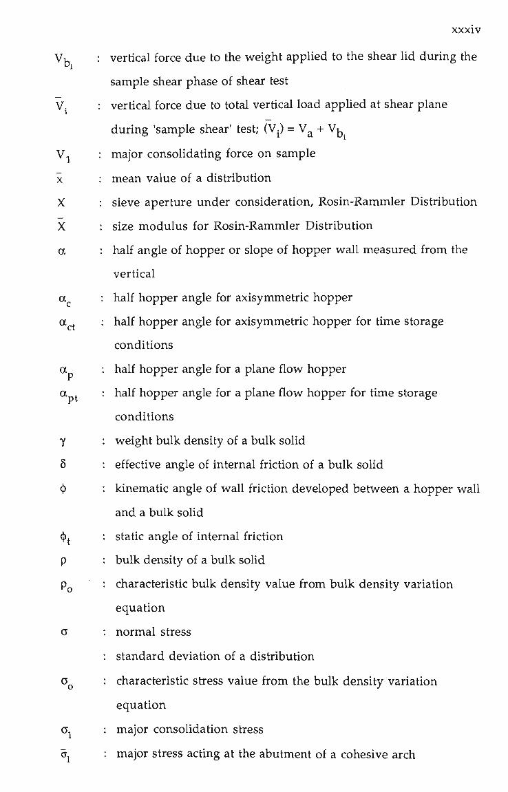
N O M E N C L A T U R E

A

b

B

B,

B ct

B.

B Pt

f

t

C

c

D

F

ff

FF

FF

g

h

H

HGI

H(a)

L

coefficient of the three parameter empirical equation

: compressibility constant exponent used to relate bulk density to

consolidation stress

: intercept of the linear empirical equation

: critical arching dimension (width or diameter) for a mass flow

hopper

: coefficient of the three parameter empirical equation

: critical arching dimension for an axisymmetric hopper

: critical arching dimension for an axisymmetric hopper under

time storage conditions

: critical arching dimension for a plane flow hopper

: critical arching dimension for a plane flow hopper under time

conditions

coefficient of the three parameter empirical equation

coefficient of the Warren Spring yield locus equation

critical piping or ratholing dimension for funnel flow

unconfined yield force under instantaneous conditions

flow factor for a converging flow channel

flow function for a bulk solid

time flow function

acceleration due to gravity

depth variable in vertical section

height of mass flow cylinder

total height of funnel flow bin

: effective consolidation head of material, funnel flow design

: Hardgrove Grindability Index

: design function of a and hopper outlet shape [1]

: length of hopper outlet slot for plane flow hopper

xxxiii

m : hopper outiet shape, axisymmetric (m=l) or plane flow (m=0)

: gradient of the linear empirical equation

n : size distribution parameter from Rosin-Rammler Distribution

: coefficient of the Warren Spring yield locus equation

: number of readings of statistical distribution

R : % weight retained on a sieve aperture, Rosin-Rammler

Distribution.

^a : the arithmetic mean of the profile height deviations of a surface

S : steady state shear force during the "shear consolidation" phase of

shear test

selected " ^^^ value of S selected for a particular level of consolidation and

used for prorating (Sj) ^ ^ values.

S. . : an uncorrected value of S determined from the shear test test

Sj : maximum value of shear force obtained during the "sample

shear" phase of the shear test

(S) ^ i'prorated

: a corrected value of Sj obtained using the prorating technique

(S.) gg : an uncorrected value of S determined from the shear test

T : coefficient of the Warren Spring yield locus equation

V : vertical force due to total vertical load applied at shear plane

during the 'shear consolidation' phase of the shear test

V^ : vertical force due to the mass of the shear lid, shear ring and bulk

solid above the shear plane (that is, contained within the shear

ring)

V^ : vertical force due to the weight applied to the shear lid during the

shear consolidation phase of shear test

V : vertical force due to the weight applied to the twisting lid during

the pre-consolidation phase of shear test

XXXIV

Vu : vertical force due to the weight applied to the shear lid during the

sample shear phase of shear test

V. : vertical force due to total vertical load appHed at shear plane

during 'sample shear' test; (V.) = V ^ + Vj j

V^ : major consoHdating force on sample

X : mean value of a distribution

X : sieve aperture under consideration, Rosin-Rammler Distribution

X : size modulus for Rosin-Rammler Distribution

a : half angle of hopper or slope of hopper wall measured from the

vertical

a : half hopper angle for axisymmetric hopper

a . : half hopper angle for axisymmetric hopper for time storage

conditions

a : half hopper angle for a plane flow hopper

a ^ : half hopper angle for a plane flow hopper for time storage

conditions

7 : weight bulk density of a bulk solid

8 : effective angle of internal friction of a bulk solid

(j) : kinematic angle of wall friction developed between a hopper wall

and a bulk solid

(|)j : static angle of internal friction

p : bulk density of a bulk solid

PQ : characteristic bulk density value from bulk density variation

equation

normal stress

standard deviation of a disfribution

Op : characteristic sfress value from the bulk density variation

equation

Oj : major consolidation stress

Gj : major stress acting at the abutment of a cohesive arch

XXXV

a : unconfined yield stress of a bulk soHd

a j : unconfined yield stress of a bulk solid under conditions of time

storage at rest

X : shear sfress

CHAPTER 1

INTRODUCTION

The quantities of Ausfralian coal, which pass through surge and

storage bins annually is considerable and continually increasing. This trend

applies not only to the coal producers and export market facilities, but to

coal users in such industries as steelmaking, electricity generation and

cement manufacture. The achievement of reliable gravity flow is essential,

particularly with the increasing size of the storage units and the automation

of bulk solid material handling and processing systems.

These trends are exacerbated when from a flow or 'handleability'

viewpoint it may be considered that the quality of coal is reducing in

present times. This is due to a number of factors, including modern coal

mining techniques and increasingly efficient froth flotation techniques in

coal preparation plants producing finer coal, and, the acceptance of coal with

higher ash contents as being a marketable proposition.

The present state of the art for the design of storage bins for

reliable flow and structural integrity require complete flow property tests to

be carried out on each new bulk solid considered. With due attention to the

bulk solid flow properties, designs often can be achieved that utilise gravity

for reliable flow. Within this scenario it would be advantageous if the

major physical variables of coal and their influence on the flow properties

were to be identified and assessed with a view to reducing the sample

testing required and developing standard design rules and rationale.

In the field of bulk solids handling it is essential that both the

storage and the discharge from storage of materials is carried out in an

effective and efficient manner. However, it is known that flow out of bins

2

and hoppers is often unreHable and as a result considerable costs can be

incurred due to the consequential losses in production. This is very often

the case with coal handling plant due to the cohesive and variable nature of

coals. Problems that commonly occur in the operation of storage bins

(including solids segregation, erratic flow, flooding, arching, piping and

adhesion to the bin wall) can reduce the bin capacity below the designed

values, or lead to flow blockages. In most cases the problems that occur in

practice are due to inadequate design analysis compounded by a lack of

knowledge or appreciation of the relevant flow properties of the materials.

All too often the design of bins and hoppers for the storage of coal has been

treated empirically with little or no regard for the relevant flow properties

and the fundamental concepts of the behaviour of bulk solids.

In recent years significant advances have been made in the

development of the theories and associated analytical procedures to describe

the behaviour of bulk solids under the variety of states that are encountered

in materials handling operations. Of particular note is the pioneering work

of Dr. A.W. Jenike and his colleague Dr. J.R. Johanson in the formulation of

comprehensive mathematical models describing the flow of cohesive bulk

solids from bins and hoppers and the required associated design procedures.

The Jenike theory has precipitated a great deal of research

throughout the world on problems associated with the storage and flow of

bulk solids. As a result there are now well established testing techniques for

the measurement of bulk solid strength and flow properties and

industrially proven procedures for bin design and evaluation.

For the purpose of providing a suitable background to the

investigations covered in this work a brief overview will presented of the

philosophy of bin design, the experimental techniques for flow property

determination and application of the flow properties to hopper design.

3

Readers are also referred to References [ 1 - 4 ] where the general theories

pertaining to the gravity flow of bulk solids in hoppers and the associated

design procedures are documented more fully.

1.1 BIN DESIGN PHILOSOPHY

The design of storage bins for bulk solids is basically a four step

process:

• Determination of the strength and flow properties of the bulk

solids for the worst likely conditions expected to occur in practice,

• Determination of the bin geometry to give the desired capacity, to

provide a flow pattern with acceptable characteristics and to

ensure that the discharge is reliable and predictable.

• Estimation of loadings exerted on the bin walls and the feeder

under operating conditions.

• Design and detailing of the bin structure.

It is important that all bin design problems follow the above

procedures. When investigating the required bin geometry, it should be

assumed that gravity will provide a reliable flow from storage. Not until it

has been demonstrated that the gravity forces available are insufficient to

provide reliable flow should more sophisticated reclaim methods or flow

aids be investigated.

1.1.1 Bin Flow Patterns

Following the definitions of Jenike, there are two basic modes of

flow, mass flow and funnel flow. These are illustrated in Figure 1.1. Each

mode has its own advantages and disadvantages and it is important that

designers and operators of bins be aware of their individual characteristics

Total capacity live

Central How channel Tendency to pipe

Dead capacity I ikiey

(a) Funnel-Flow lb) Mass - Flow

Figure 1.1 Flow Patterns in Symmetric Funnel Flow and

Mass Flow Bins.

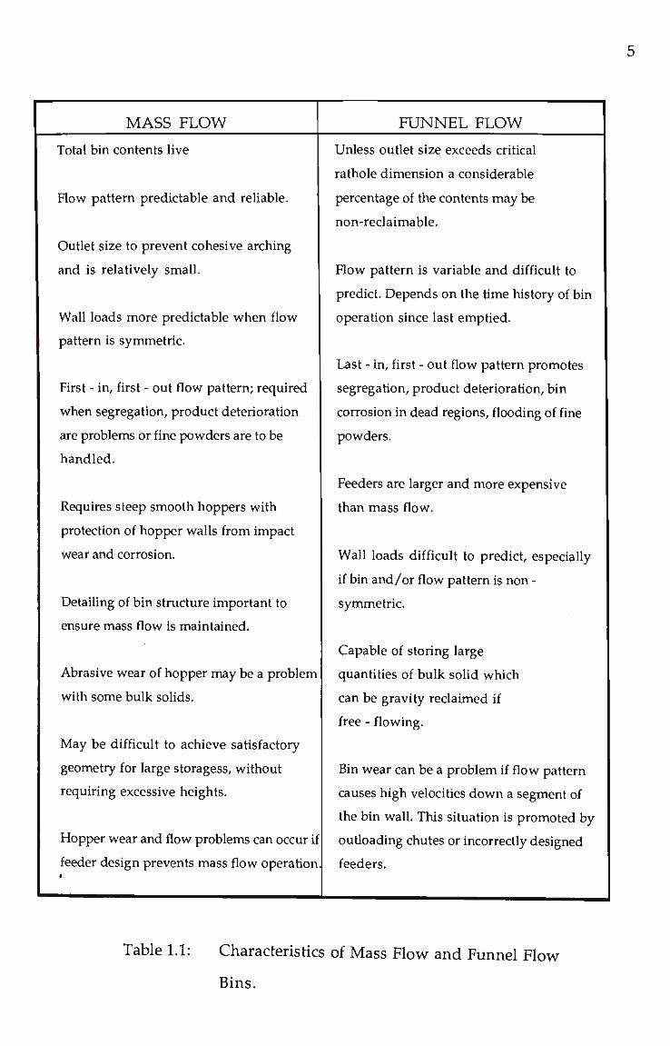
MASS FLOW FUNNEL FLOW

Total bin contents live

Flow pattern predictable and reliable.

Outlet size to prevent cohesive arching

and is relatively small.

Wall loads more predictable when flow

pattern is symmetric.

First - in, first - out flow pattern; required

when segregation, product deterioration

are problems or fine powders are to be

handled.

Requires steep smooth hoppers with

protection of hopper walls from impact

wear and corrosion.

Detailing of bin structure important to

ensure mass flow is maintained.

Abrasive wear of hopper may be a problem

with some bulk solids.

May be difficult to achieve satisfactory

geometry for large storagess, without

requiring excessive heights.

Hopper wear and flow problems can occur if

feeder design prevents mass flow operation.

Unless outlet size exceeds critical

rathole dimension a considerable

percentage of the contents may be

non-reclaimable.

Flow pattern is variable and difficult to

predict. Depends on the time history of bin

operation since last emptied.

Last - in, first - out flow pattern promotes

segregation, product deterioration, bin

corrosion in dead regions, flooding of fine

powders.

Feeders are larger and more expensive

than mass flow.

Wall loads difficult to predict, especially

if bin and/or flow pattern is non -

symmetric.

Capable of storing large

quantities of bulk solid which

can be gravity reclaimed if

free - flowing.

Bin wear can be a problem if flow pattern

causes high velocities down a segment of

the bin wall. This situation is promoted by

outloading chutes or incorrectly designed

feeders.

Table 1.1: Characteristics of Mass Flow and Funnel Flow

Bins.

as these can have a significant effect on bin performance. Some of these

characteristics are summarised in Table 1.1. In mass flow the bulk material

is in motion at substantially every point in the bin whenever material is

drawn from the outlet. The material flows along the walls of the bin and

hopper (ie. the tapered section of the bin) forming the flow channel. Mass

flow occurs when the hopper walls are sufficiently steep and smooth and

there are no obstructions to flow, such as abrupt transitions or inflowing

valleys.

Funnel flow (or core flow), on the other hand, occurs when the

bulk solid sloughs off the surface and discharges through a vertical channel

or pipe which forms within the material in the bin. This mode of flow

occurs when the hopper walls are rough and the slope angle (a) is relatively

flat. The flow is erratic with a strong tendency to form stable pipes which

obstruct bin discharge. When flow does occur, segregation takes place, there

being no remixing during flow. It is an undesirable flow pattern for many

bulk solids, however, it has advantages of minimal bin wall wear, being less

costly and having reduced height requirements than for similar tonnage

mass flow designs.

Mass flow bins are classified according to the hopper shape and

associated flow pattern. Typical mass flow bins are shov^m in Figure 1.2. The

two main types are conical hoppers, which operate with axisymmetric flow,

as in Figure 1.2(a), and wedge-shaped or chisel-shaped in which plane flow

occurs, as in Figure 1.2(b). In plane flow bins the hopper half angle a is

approximately 10 larger than that for corresponding conical hoppers.

Therefore, they offer larger storage capacity than for a conical hopper for the

same headroom, although this advantage is sometimes offset by the long

slotted opening which can cause uneven feed problems. The transition

hopper, which has plane flow sides and conical ends, offers a more

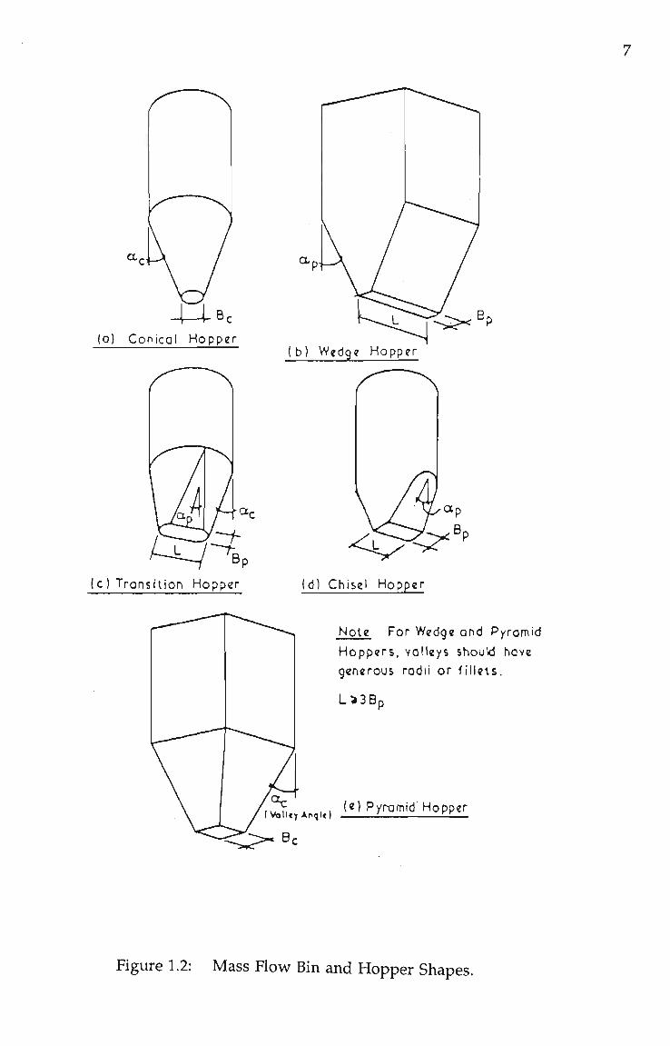
(a) Conical Hopper

(c) Transt'iion Hopper

b) Wedge Hoppgr

(d) Chisel Hopper

Note For Wedge and Pyromid

Hoppers, volleys should hove

generous rodii or f i l le ts.

L i3B„

,~^. . ,. (e) Pyramid Hopper I Vollf| Af>ql«l '- L-L

Figure 1.2: Mass Flow Bin and Hopper Shapes.

8

acceptable opening slot length, and allows bin diameters larger than slot

outlet length. Pyramid-shaped hoppers, while simple to manufacture, are

undesirable in view of the build-up of material that is likely to occur in the

inflowing valleys which represent high wall friction regions.

The limits for mass flow depend on the half angle a, the wall

friction angle (j) and the effective angle of internal friction 8. In the case of

conical hoppers the limits for mass flow are clearly defined and quite

severe, as illustrated in Figure 1.3. Plane flow or wedge shaped hoppers

have similar limits for mass flow but these are much less severe [3,41.

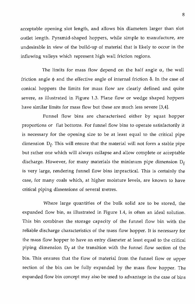
Funnel flow bins are characterised either by squat hopper

proportions or flat bottoms. For funnel flow bins to operate satisfactorily it

is necessary for the opening size to be at least equal to the critical pipe

dimension D . This will ensure that the material will not form a stable pipe

but rather one which will always collapse and allow complete or acceptable

discharge. However, for many materials the minimum pipe dimension Dc

is very large, rendering funnel flow bins impractical. This is certainly the

case, for many coals which, at higher moisture levels, are known to have

critical piping dimensions of several metres.

Where large quantities of the bulk solid are to be stored, the

expanded flow bin, as illustrated in Figure 1.4, is often an ideal solution.

This bin combines the storage capacity of the funnel flow bin with the

reliable discharge characteristics of the mass flow hopper. It is necessary for

the mass flow hopper to have an entry diameter at least equal to the critical

piping dimension D£ at the transition with the funnel flow section of the

bin. This ensures that the flow of material from the funnel flow or upper

section of the bin can be fully expanded by the mass flow hopper. The

expanded flow bin concept may also be used to advantage in the case of bins

I I I I I I I II I I I I I I — I I I I I — 1 — I I I I — 1 — I — I — I I ' ' ' I ' ' ' ' I ' ' ' ' I

en az UJ Q-Q_ o X

(n oc UJ Q_ Q_ O H

o

(S

ID CO C9 CS3

S33yD3a - NOIiDiyj 11BM JO 310NB 3IitiW3NIM

Figure 1.3: Wall Slope Limits for Mass Flow in

Axisymmetric and Plane Flow Hoppers.

10

Flaf or Conical

Flow Ftitterns

Figure 1.4: Flow Pattern in a Symmetric Expanded Flow

Bin.

11

or bunkers with multiple ouflets providing the design and operation

ensures that the flow channels of adjacent ouflets merge.

1.1.2 Determination of Flow Properties of Bulk Solids

In order to design storage bins and associated handling systems it is essential

that the flow properties be determined by the testing of a representative

sample. The sample tested consists of the fines of the bulk solid, usually the

-2.36mm or -4.00mm fraction. This approach is taken because it is

considered that the cohesive strength of a bulk soHd can be attributed to the

fines content. For a material to shear and flow the cohesive strength of the

fines must be exceeded to allow the shearing action between the coarser

fraction to take place.

The following flow property tests provides the designer with such

parameters as:

• Flow Functions (FF) for instantaneous and simulated time

storage conditions at rest for low and high consolidation

pressures. The flow functions provide a graphical representation

of the variations in bulk solid strength with the changes in major

consolidation stress occurring under storage and flow conditions.

• Effective Angle of Internal Friction (8),

• Static Angle of Internal Friction (^^).

• Kinematic Angle of Wall Friction ((j)) for different bin wall

materials and surface finishes.

• Bulk Density (p) as a function of consolidation pressure.

The flow properties Hsted above are determined using a Jenike-type Direct

Shear Tester except for the bulk density variation which is determined

using the Jenike Compressibility Tester. The flow properties are generally

expressed as a function of the major consolidation stress or pressure since

design procedures to determine critical bin and hopper geometries take

12

account of the variation with major consolidation stress. Figure 1.5 presents

the general form and trends of the flow properties with major consolidation

stress. Details of the procedures used for flow property testing are given in

References [3,4].

1.1.3 Determination of Bin Geometry

Once the various flow properties have been obtained it is then

possible to determine the required bin shape to provide mass flow, funnel

flow or expanded flow.

Based on the operating constraints and the bulk solid

characteristics indicated by the flow properties, the particular form of storage

bin must be decided. Often in more recent times, industry has required the

design of new storage facilities to provide mass flow operation. This is a

misconception; funnel flow or expanded flow concepts can be successfully

utilised provided attention is paid to the principles of bulk solids flow and

the relevant flow properties. The use of mass flow facilities is more

expensive than a corresponding funnel flow installation in terms of the

required headroom for a given volume (due to the steep hopper walls), the

installation of low wall friction liners in the hopper, the high stress

loadings at the transition and often higher feeder loadings, and the extra

attention required for the construction, installation and maintenance of the

internal surfaces.

A decision flow chart has recently been developed by Carson [51,

and is presented in Figure 1.6. This procedure details the correct priority of

the available design options to ensure the most economical storage facility

is achieved. Unfortunately, for the handling of coal, particularly with high

fines content and moisture content the extremely large ratholing diameters

13

^ 1000

i?^ 900

!::: 800 to

1 700

S 600

60

c§ 50

^ 40

50

40

^ 30

20

10

25

•^ 20 to to

S 15 to

9 g 10

1 3 5:

-

-

-

1

1 1

1 1 1 1 I I 1 1

-

1 1 1 1 1 1 1 1 1 1 1 1 1 1 1 1 • '

-—— . s

r 1 1 1 1 1 1 1 1

"V

1

1 1

1 ,, .

1 1 1 1 1 1 1 1

^RUSrr MILD STEEL

--••• PACTENE

^304 2'B STAINLESS STEEL .

1 1 1 1 1 1 1 1 1 1 1 1 1 1 1 1

i DAY TIME FLOW FUNCTION.,^^^^^^^ ""'^

^^'^^^^^^^^^-^"^'^^INSTANTAHCOUS FLOW ^^^;:::^>^^ FUNCTION

1 1 1 1 1 1 1 1

10 15 20 25 30 35 40 45 MAJOR CONSOLIDATION STRESS-kPa

50

Figure 1.5: Typical Coal Flow Properties.

14

Is segragqtion linportgnt? |-

m. -nye^

Uill tho malarial degrade with extended gjorage time?

Cno^

is the fines level greater than 10^ through a 150 XM (. 100 mash) screen? -•ruea

Is accurate feed rate con troI i mpor tanI? -(MD-

ITpy the Funnel Flow Btn Design Procedure |

I Is the required feeder size adequate for your flow rate?

cm

Vou likely have the least costly bin design for this material.

fit an affective head of 3m <I0 ft>, is the critical rathole greater than 3ni < 10 ft)?

^p Mill moderate segregation cause process problems?

Cnp Can the bin I eve I be Iowered per i odIca11y to ensure movement of ai i material?

C ^

v _ J ^^^ Expanded Flow Bin "^—' Design Procedure.

Dse Doss Flo« Bin Design Procedure as t h i s is tlie only type of b in for I t i i s m a t e r i a l .

Is the out le t large enough to provide the maxImum required discharge rate? -Cno>

Enlarge the outlet or use an air permeation system.

^

Is the lowest speed of the selected feeder reasonable for the flow rote required?

s. <MD-

Vou likely have the best bin design for this material.

Repeat the design procedure using the continuous flout properties of the material with an overpressure factor of at least 25Ji. Use i\om aids to dislodge material after lime of storage ot rest. This will allow the use of a smaller feeder thus Increasing Its speed.

Figure 1.6: A Procedure to Design Bins and Feeders

(Carson[5]).

15

encountered and the threat of spontaneous combustion, usually precludes

the use of funnel flow designs. For these reasons the design procedure for

funnel flow bins will not be included. Details on funnel flow design are

presented in References [3, 41.

1.1.4 General Design Procediu-e for Mass Flow Geometry

The aim of mass flow design is to determine the hopper

geometry, in particular the hopper half angle a and the opening size B, so

that a stable cohesive arch cannot form over the outlet and that the entire

contents of the bin are in motion when discharge occurs. Two parameters

are important: firstly the 'flow function', FF, representing the strength of

the material as previously described, and secondly the 'flow factor', ff,

which describes the stress condition in the hopper during flow. The flow

factor is given by:

ff = =r (1.1) ^1

The flow factor is represented as a ray from the origin (with a -1 ^1

slope of tan ( — )), and is shown, together with the flow function, in Figure

1.7. The flow factor depends on the wall friction angle (|), the hopper half

angle a and the effective angle of internal friction 5. The determination of

the flow factor is described in Reference [31 which also presents the

associated flow factor charts.

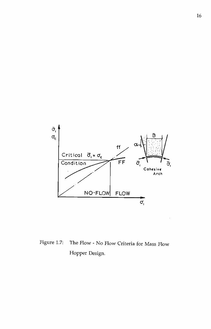
By utilising a flow-no flow concept (Figure 1.7), the stiength of the

bulk solid (as represented by the flow function), is compared with the

stresses imposed by the hopper (represented by the flow factor). Referring to

Figure 1.7, flow will occur when the major stress acting at the abutment of

the cohesive arch o^ imposed by the hopper exceeds the unconfined yield

stress of the bulk solid o^ causing the cohesive arch to fail.

16

5,' a.

c

1

Critical 5, = cr .

Con d it io n ^^ ..-- ;;;;

y^y^

y ^ NO-FLOW

i\ y

^^'^

?\sy^

<M I B

^^j^azzaoii /

^ . 0-. Cohesive

Arch

Figure 1.7: The Flow - No Flow Criteria for Mass Flow

Hopper Design.

17

The critical value of a^ occurs at the intersection point of the flow factor and

the flow function. If the flow properties of (]) or 6 vary with CT^ an iterative

procedure must be carried out until Oj converges to the critical value.

The minimum outlet dimension B is defined by:

B = ^ l 2 ^ = ( | ) ^ (1.2) Pg " Pg

The function H(a) depends on the ouflet shape and hopper half

angle a and is presented graphicaUy in Reference [3]. In practice the opening

size should be made larger than the above calculated minimum value of B

in order to achieve a required flowrate or to allow a degree of conservatism

for variation in the bulk solid flow properties from those tested. Variations

in material flow properties due to moisture content and storage time can

significantly influence the hopper geometry.

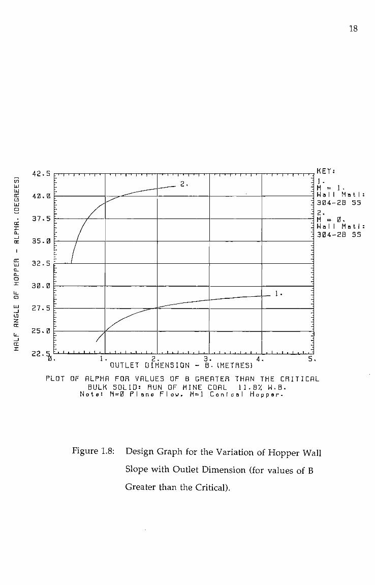
It is common for wall yield loci to have a convex upward curved

shape. This leads to a angle of wall friction that is pressure dependent as the

major consolidation stress o^ increases, the wall friction angle (^ decreases.

Since the major consolidation stress increases with the distance measured

upward from the hopper outlet, advantage may be taken of the

corresponding decrease in (j) by increasing the hopper half angle a . This

characteristic can also be exploited by increasing a for increasing outlet span

of the hopper as required by other design constraints, A design graph

detailing the variation of a with B trend is presented in Figure 1.8 for a

typical black coal.

1.2 CONCLUDING REMARKS

This study investigates two major aspects of the design procedures

for mass flow storage facilities for hard black coal. The first involves

assessment of the degree of influence of various physical variations of coal

18

hi

az LU

a

tx 0_

UJ Q-0 . O X

u. a tu _j u z cr

en X

4 2 . 5

4 0 . 0

3 7 . 5

3 5 . 0

3 2 . 5

3 0 . 0

2 7 . 5

2 5 . 0

22 . %

: - i - | 1 1 1 1 i - r '

lllllllll

ll

ll

ll

ll

l

r /

ll

ll

ll

ll

l lllllllll

'I'I

'I'I

'

I / • . 1 . 1 . 1 . 1 .

• I ' I ' I ' I '

/ - ^

• I •

1 f 1 1 1 1 i - i I

2 .

I . l .

' I ' I ' I ' I '

• 1 • '

- 1 1 > 1 I I 1 1 1 .

lllllllll

ll

ll

ll

ll

l l

ll

ll

ll

ll

-i 1

ll

ll

ll

ll

l l

ll

ll

ll

ll

• 1 . 1 . 1 . 1 . "

K E Y :

~- 1 M = 1 . Wal I H a t I : 3 0 4 - 2 B SS 2 . M = 0 . No! I M a t t : 3 0 4 - 2 B S3

OUTLET DIMENSION - B". (METRES) 5.

PLOT OF RLPHR FOR VRLUE5 OF B GRERTER THRN THE CRITICAL BULK SOLID: RUN OF MINE CORL 11.8X W-B.

Note! M=0 Plane Flow. M=l Conical Hopper.

Figure 1.8: Design Graph for the Variation of Hopper WaU

Slope with Ouflet Dimension (for values of B

Greater than the Critical).

19

samples on the subsequent flow properties. Flow property testing can be

quite time consuming and expensive, particularly for large testing

programs, (as might be required for a storage bin at an export coal loading

facility). Identification of the most influential parameters will thus reduce

the testing required and allow the development of standard hopper design

rules.

The second aspect addressed is the current design procedures

used in the determination of mass flow hopper geometries. Although this

technology has now been available for the past thirty years, utilisation and

exposure to industry has been limited, due to somewhat complicated

manual design procedures or the inability to effectively apply computer

techniques. This work details the development of manual hopper design

nomograms and computer aided design programs to help address the

abovementioned shortcomings.

Literature surveys of relevant published material have been

included in the respective chapters to aid the continuity and presentation of

this study.

20

CHAPTER 2

EXPERIMENTAL INVESTIGATION OF THE FLOW

PROPERTIES OF BLACK COAL

2.1 INTRODUCTION

This study is concerned with the flow properties of hard black coal

which make up the major portion of Australia's steaming and coking coals

for the domestic and export markets. Coals below the rank of

sub-bituminous, such as brown coal and lignite will not be included.

The literature survey conimences with published literature prior

to development of the Jenike theories through to the present.

2.2 LITERATURE SURVEY AND IDENTIFICATION OF

VARIABLES

The handling and storage of coal has always presented industry

with problems of unreliable flow, spasmodic feeding and blocking of bin

outlets. For many years solutions to these problems were based on

mechanical devices, ranging from sledge hammers and air lances through

to vertically moving chains and vibrators. Presented below in chronological

order is a review of the literature detailing past studies with special

reference to papers concerning coal handling studies.

Early attempts of measuring the physical properties of coal were

frustrated because no general theory of gravity flow had been developed and

the application of soil mechanics testing equipment was too insensitive to

quantify the small stresses acting in cohesive arches. As a result, studies

such as those of Wolf and Hohenleiten [6] and Legget [71 concentrated on the

use of models to explore the mechanics of bulk solid storage and flow, most

findings generahy being inconclusive. However, these studies did identify

21

the importance of the surface moisture content and the fines content of coal

in leading to flow blockages. This agreed with findings in industry, for

example Legget notes that flow blockages occurred at the plant in question

after a certain moisture content was exceeded (6%). The bins used during

this era were generally of the funnel flow design, and commonly had

asymmetrically located outlets. Because these designs were far outside the

regions of mass flow (Figure 1.3) complete emptying would often not occur

for any combination of bin lining material, outlet dimension or the

addition of vibrators. With regard to improving the flow of coal from

bunkers before the development of the Jenike theory, one finds in the

literature such comments as 'the slope of the hopper is not a determining

factor' and 'expensive bunker linings are unnecessary since they do not lead

to flow [71

A notable study conducted on the handling of coal smalls was

reported by Hall and Cutress [8]. This study was hampered similarly by the

non-existence of a theory of gravity flow and sensitive laboratory

instruments. In measuring the fundamental physical properties of several

coals by triaxial tests, the results indicated only slight differences, for

materials which were known to behave quite differently in practice. Since,

previously,there had not been a standard method of measuring handleability,

they developed what has become known as the Durham Cone Index. This

index is equal to the time required to empty a small vibrated conical

hopper, the results for a given sample being found to be reproducible. The

tests also indicate, for different samples, significant differences in the

measured index corresponding to the known differences in the flow

properties of the respective samples. Variables of the coal samples

considered included the fines content (-500 |im), the moisture content, the

rank of the coal and the effect of addition of some quantities of oil.

Conclusions noted from the study in terms of the Durham Cone Index were

that for all coals tested the discharge time increases with moisture content

22

to a maximum then decreases, and the value of the maximum time reduces

and occurs at a lower moisture content with decreasing rank. Decreasing the

fines content decreased the discharge time to empty at all moisture contents

and considerably reduced the maximum value.

In addressing the observed trend of discharge time with moisture

content^ the authors provide a qualitative explanation in terms of the levels

of moisture film between the coal particles, ie. the variation from the

pendant to funicular condition and from funicular to capillary states of

moisture.

Although the Durham Vibrating Cone is still used, the method

only gives an indication of flowability for comparison between samples

where only one variable is changed. It is difficult to quantify the effect of

two or more variables on the samples' flowability. For the method to have a

more practical use^ a background of experience is required to relate the

discharge time from the vibrating cone to actual plant performance.

Two recent studies, Mikka and Smithan [91 and Crisafulli et al.

[101 have utilised the Durham Cone in assessment of coal handleability of

Australian black coal. In the case of Mikka and Smithan, the influence of

moisture content, particle size distribution, mineral content and coal

preparation matter reagents on handleability were investigated.

Considering the influence of coal particle distribution the handleability was

assessed by both the Jenike shear cell (assessment based on outlet dimension

B^ of a conical stainless steel bin) and the Durham Cone (assessment based

on discharge time). This study concluded the most significant variable

affecting the handleability of washed coal to be the particle distiibution. For

coals containing little or no fine particles (-500iim), handleability was found

to be insensitive to moisture content. However, at high levels of fines the

handleability was found to be extremely sensitive to moisture content.

23

Investigations by Crisafulli et al. [101 used the Durham Cone to

assess the extieme effect of moisture content on the handling of Walloon

coal from Queensland. This coal was particularly difficult to handle for

moisture contents above 9%, due to the high clay content (bentonitic types)

and its friable nature (Hardgrove Grindability Index, HGI, of 33).

At around the same period of the work of Hall and Cutress, Jenike

was developing his theory of gravity flow and the required experimental

procedures to measure the flow properties. These are covered in the

University of Utah Engineering Experiment Station Bulletins [1-31. A major

feature in the work of Jenike is the testing of the fines, justified by

recognising that the large particles move bodily while the material shears

across the fines. The coarse particles are a passive agent which do not

develop shear strength without the fines to bind them. He also stipulated

testing of the worst representative sample, in terms of physical parameters

such as moisture content, temperature and time storage at rest, to

determine the flow properties for bin design.

Using an annular shear tester (as compared to the direct shear

tester of Jenike). Jones [11] applied the theory of Jenike in investigating the

factors of moisture, particle size and ash content on the flow properties of

several British coals. His results indicated the most significant factor to be

the fines content (-63 |im considered) with ash content and moisture

(moisture content ranging from 0.5 to 7.6% free moisture only considered)

having negligible effect. Although this study was also designed to establish a

reliable handleability index, and, considered the Durham Vibrating Cone,

the flow function FF (from Jenike) and the Power Index 'n' (from the

Warren Spring Equation describing yield loci) no recommendations were

presented except to indicate disadvantages of the Durham Cone discharge

time.

24

A report compiled by Foster-Miller Associates [12] in 1981,

considering the increase of effective bulk density of coal nune car loads by

vibration included a section submitted by Jenike and Johanson Inc. on the

results of flowabUity tests of the coals considered. For comparison of the

tested coals, the flowability was expressed as the mmimum ouflet diameter

required for a conical mass flow bin for unobstiucted flow. This provided a

useful index which can be readily related to existing plant designs. The

signiflcant effect of moisture content on the flowabflity of coal was noted.

From a series of tests on two coals for a range of moisture contents, the

flowablHty varied from free-flowing for moisture contents below 5%, to

required ouflet dimensions of 4 to 7 feet in diameter for unobstructed flow

at the higher levels considered (15 - 22%).

It is apparent from the literature that moisture content is a major

factor affecting the flowability of coal. As stated by Royal and Costello [13]

only the surface moisture of coal directly affects the cohesion and friction

parameters. They considered methods of measuring the surface moisture of

coal (including air drying, heated ventilated oven and microwave) and

included preliminary correlations between surface moisture and the flow

properties of three coals (of lignite, sub-bituminous and bituminous rank).

Findings of the report state no correlation was found between surface

moisture and the flow test data. However, it is considered that this was due

to the wide range of coal rank considered and the low moisture levels

considered (typically 0 - 4% surface moisture). An important aspect raised in

[13] was the action of weathering and slacking, where coals stored in

stockpiles achieving a marked decrease in flowability over time.

The flow properties of Australian coals has recently been

investigated by Leung and Osborne [14]. They determined the flow

properties of four coals, namely, Tarong, Millmeran, Callide and Blackwater

using a Jenike Direct Shear Tester. The major conclusions noted were the

25

significant effect on the flow properties of the moisture content (7 - 21%

considered). the sample fines content (-212 |im) and the period of

consoHdation at rest (2 days considered). It was also reported that the

method of crushing should have no effect on the flow properties since litfle

difference in particle sphericity could be measured between particles

crushed by jaw and roller crushers. From a comparison of the four coals

considered, Blackwater presented the stronger coal, with no significant

differences between the other three.

Further consideration of the effects of moisture on the handling

of coal has been investigated by Day and Hedley [15] who developed a

computer simulation model. They noted from previous studies that

cohesion increases, passes a maximum and decreases as a function of

increasing moisture content. The computer model has enabled the cohesion

effects to be quantified in terms of the particle distribution and the angle of

contact between the water surface and the granular material.

A study [16] for the ETSI pipeline project in the USA (concerned

with the slurry transport of sub-bituminous coal), considered the handling

and storage problems of dewatered coal. Due to the fine particle sizing (finer

than comparable railed coal) and the moisture content it was realised

significant levels of cohesive strength could be achieved and must be taken

into account when designing bin and hopper outlets. The dewatered

pipeline coal had a design surface moisture content of 9 - 10% and particle

distributions of up to 23% passing a 45|im sieve. Lower moisture contents

could not be tolerated due to dust problems. Flow property testing of the

coal for increased moisture contents levels showed an increasing trend of

hopper outlet dimension for both instantaneous and time storage

conditions ranging from 1 foot to 4 feet diameter for 18%.

26

The effectiveness of chemical additives to enhance the flow

characteristics of coals under high moisture contents was also investigated.

Considering water absorbent polymers (which reduce the apparent surface

moisture) and surfactants (which reduce the cohesive strength of the water

film binding particles) both were found to effectively improve flow of coal

from hoppers. However, in view of their expense they were considered

unwarranted as the relevant flow property variation had been taken into

account in the design of the hoppers.

Reviewing the above literature, the most influential variables

appear to be the free surface moisture content, the particle distribution

(more specifically the fines content) and the time storage at rest. This

concurs with experience gained from industry. Variables affecting the flow

properties of coal can be considered under two groups, the physical

characteristics of coal and secondly, the characteristics imposed on the coal

from operating conditions and equipment. The first group includes the

variables of coal rank, maceral constituents, particle shape and ash content.

Variables that can be considered under the second grouping of

external influences include the use of chemical additives (for dust

suppression or increased flowability), time consolidation at rest, the

addition of moisture, the industrial processes of mining, washing and

crushing in determining the particle sizing, and the variation of different

angles of wall friction for different lining materials (a change of only a few

degrees can lead to the discharge pattern changing from mass flow to funnel

flow).

Arnold et al [17] recently completed an extensive testing program

to determine the influence of several of the above variables on the flow

properties of black coal from the Soutiiern Coalfield, Sydney Basin of New

South Wales. The experimental results were also applied to the

27

determination of the mass flow hopper geometry parameters of hopper

slope and outlet span allowing the influence of the variables to be further

assessed. The most significant variables were found to be the moisture

content, particle top size of test samples and time consolidation at rest.

The most recent and comprehensive review of the available

literature relating to the successful handling and storage of coal has been

compiled by Wood [18], The major findings of this report are that moisture

content and particle size are the major variables affecting coal flowability.

These two factors influence considerations such as the packing of the coal

particle assembly, size segregation during storage and flow.

Obviously the difference in flow properties between lignite and

anthracite requires no clarification; however, the variation caused from the

changes in rank from sub-bituminous, high volatile bituminous, medium

volatile bituminous and low volatile bituminous is more difficult to

identify. The variations of particle shape, constituents and friability are

interrelated due to the over-riding influence of the physical characteristics

of the macerals on such properties. The identification of these trends is

made more difficult because of the heterogenity of the coal constituents,

such that no general trends can be observed between coal basins, between

coal seams or, in extreme cases, the daily operation of mines,

2.3 A BRIEF DISCUSSION OF THE ILLAWARRA COAL MEASURES

Coal samples from the Southern Coalfields (Illawarra Measures)

of New South Wales were used for the flow property testing program to

assess the influence on the flow properties of the various factors

highlighted by the literature survey.

The Illawarra coal measures cover the south-eastern segment of

the well known Sydney Basin. Geologically the coal measures are of

28

Permian Age [19] and lie on the Shoalhaven group with Triassic rock

covering the coal. The measures form what is known as the Southern

coalfields and range in thickness from less than 150 metres in the south

near Dapto to over 300 meties in the north at Helensburgh [20,21]. Referring

to Figure 2.1 where it can be seen that there are many coal seams in the

measure, only four however are mined commercially; namely the Bulli,

Balgownie, Wongawilli and Tongarra Seams [22].

Characteristics of each of the coal seams are as follows [20,23].

• Bulli. This seam is identifiable over most of the coalfield and is

the most extensively mined. It consists essentially of clean coal

reaching 4 metres thick in the north and thinning to 0.3 metres in

the south. The coal produced is a low volatile type with medium

to high ash content. It is a prime coking coal and is categorised [24]

as SAA No. 4a22(2) to 4b43(3).

• Balgownie Consists of unhanded clean coal reaching over 1.5

metres thickness in the extreme north east but steadily decreases

to less than 0.3 metres south of Macquarie Pass. The coal from this

seam is a prime coking coal, low to medium volatile type with

medium ash content. It is categorised as SAA No. 4A43(2) to

4b43(2).

• Wongawilli This seam extends over the whole coalfield and

ranges in thickness from 6 metres in the south to 15 metres in the

north-east however, over most of the southern coalfield it is in

the range of 9 to 10.5 metres. The seam consists of coal plies of

varying qualities separated by bands of carbonaceous and

tuffaceous shales. The coal gained from this seam is a medium

volatile coking coal, with medium to high ash content. It is very

reactive and ideally suited for blending in large proportions with

high rank coking coal. It is classified as SAA 4B44(3) to 634(4).

29

SOUTHERN

in UJ

cr

< LU

<

o

<

<

< _ j

CL

O Q:

I

m

z Q >-

a. D O cc I

CD

(/)

Q Z < _J cc LJJ CD

o

BULLI S E A M ^ BALGOWNIE SEAM

WONGAWILLI SEAM

AMERICAN CREEK SEAM

TONGARRA SEAM

u. -i

WOONQNA SEAM g

CORDEAUX SEAM •¥

7r--V UNANDERRA

SEAM

•fv-

Figure 2.1: Stratigraphic Cross-Section of the lUawarra Coal

Measures of the Southern Coalfields [20].

30

• Tongarra This seam is a base member of the Illawarra coal

measures and varies in thickness from 1.2 to 6.7 metres. It is best

developed in the Tongarra-Avondale areas. The coal is of a low to

medium volatile type with medium to high ash content (below

20%). It is a stiong coking coal.

The coal from the Southern Coalfields has the highest rank in

New South Wales and as such is in high demand for both the local steel

industry and for export markets [22]. The coal is of a bituminous rank,

although in some areas higher rank coals exist. The coal rank increases

slightly from the south to the north of the coalfields [25].

The Illawarra collieries from which coal samples were obtained

(locations are detailed in Figure 2.2) are listed in Table 2.1, along with the

respective coal seams mined. As indicated in this table, most coals tested

were Run of Mine (ROM) samples collected from the raw coal circuit,

usually after the primary breaker.

2.4 SAMPLE PREPARATION AND FLOW PROPERTY TEST

SPECIFICATION

For convenience of sample collection and to remove such

considerations as rank variation and ash content (to some extent) from the

test program, coals from the Illawarra region were considered initially.

From each colliery sampled, up to three major sub-samples were divided

and prepared for testing. The following sub-samples were prepared: 100%

minus 1.00mm, 2.36mm and 4.00mm. Considerations for the selection of

these particle top sizes were:

• The -2.36mm sample was utilised as a datum measurement, since

this is the present standard top size used for the flow property

testing of bulk solids.

31

Loadcrt •hvfi"'"""\ c««i

I. k'embla

.-.r... . - ^ "V.*Jshellharbour -^Ibion Parl?^ / \ « ^ ^ 5 ^ ) ,

CO

Railways - Private Shown thua on i i t i i i i o do Public • ! 1 I .

Hiflhwava • H M ^ H M Other Roads M M I M M Location of Collieries 9°^(^ *• W^l^

LOCATION OF COLLIERIES NEW SOUTH WALES

D»N. FR 10*TI 4-6-71

tFW. J |DWt30-6-8C APPHOVtO FTR

JOINT COAL BOARD

PLAN N? DS-200" iHirr 1 OF I tHim

Figure 2.2: Location of CoUieries where Coal Samples were

obtained for the Flow Property Testing Progam

[23]

32

Colliery

Coalcliff

South Bulli

Huntley

Metropolitan

Appin

Westcliff

Coal

Product

Run of Mine

Run of Mine

Run of Mine

Run of Mine

Seam

BuUi

Bulli and Balgownie

Run of Mine and Product

Wongawilli

BuUi

Bulli

Bulli

Table 2.1 Details of Coal Samples used in the Flow

Property Testing Program.

33

• In recent times a tiend has developed using a sample top size of

-4.00mm to allow a less conservative assessment of the flow

properties. It is assumed that the larger particle size does not effect

the validity of shear measurements. This sample top size has

particular application in the testing of bulk solids that have a

wide range of particle sizes as would occur for ROM coal.

Comparison with the -2.36mm results would be useful in

highlighting relative trends with the -4.00mm results.

• The finer fraction sample was included to indicate the trends in

the flow properties for bulk solids with high proportions of fines.

The -1.00mm sample was considered as providing a realistic

upper bound for wall friction values and the flow functions. This

trend of finer coal is occurring in industry due to changes in

mining and coal preparation techniques. As noted by Nicol et al.

[26] the current trends indicate that fine coal (-0.5mm) now makes

up the greater proportion of raw coal output in some instances

up to 40% of preparation plant feed.

The sized sub-samples were generally tested at four different total

moisture contents (expressed on a wet basis): Air Dried (generally 1 to 2.5%),

6%, 10%, and 15%. For the coals tested, it was generally found that above

15% moisture content the samples became saturated, with free water

drainage. Also, 15% was generally the upper limit of moisture content for

commercial handling operations for hard black coal.

The following flow property tests were carried out on individual

coal sub-samples. Using a Jenike-type Direct Shear Tester:

• Instantaneous yield loci to provide the instantaneous flow

function and effective angle of internal friction (5).

34

• Time yield loci to provide the time flow function for a specified

time of consolidation at rest and the static angle of internal

friction ((]).). The standard time consolidation period for tests was

72 hours.

• Wall yield loci to provide the kinematic angle of wall friction

between typical bin wall materials and the bulk soHd. Typical

materials included rusty mfld steel, bright mild steel, bright

stainless steel (304-2B) and Pactene (UHMW Polymer). The wall

friction tests undertaken were for instantaneous conditions only,

and did not attempt to determine changes in wall friction due to

either time consolidation at rest or deterioration of the wall

surface when in constant contact with the coal.

Using the Jenike Compressibility Tester:

• Bulk density as a function of consolidation pressure

The particle size distributions of the samples were determined by

sieve analysis using the procedures detailed in BS 1796 : 1952 [27]. A sieve

analysis was conducted on the as received coal sample before any sample

dividing occurred. For preparation of the sub-samples, the as received

sample was brought to an air dried condition prior to being divided into the

required number of samples by the Cone and Quartering technique to

ensure samples had essentially the same particle distribution. Each sample

was then sieved to provide the required top size of the particle distribution.

In the preparation of the samples no grinding or crushing was carried out to

generate more fines, or to bring the sample within the required top size.

It must be noted that although the samples had the same top size,

variation existed in the actual particle distributions between colliery

samples. This is in accordance with current flow property testing practices

where the sample is prepared by removing that part of the material larger

35

than the required top size and the remaining distribution is tested in its as

received distribution. At a latter stage, effort was directed to ensuring the

same particle distribution and moisture contents were similar between

different samples.

The particle distributions of the coal samples tested are presented in

Rosin-Rammler Distribution format in Figures B.l to B.24, including the as

received coal sample particle distribution. The Rosin-Rammler Distribution

has the characteristic form:

R = 100e U J (3.2)

where

R = % weight retained on sieve aperture

X = sieve aperture under consideration

X = the size modulus

n = the size distribution constant.

A major advantage of the Rosin-Rammler Distribution is that for

broken coal, sieve data can be represented by a straight line and notated by

the two parameters X and n. This distribution form was derived to model

the brittle fracture of isotropic materials such as coal, providing no sieving

and no size separation has occurred. A disadvantage, however, with this

distribution form is that experimental scatter is always reduced by taking

logarithms, and so taking logarithms twice can lead to inaccura te

conclusions regarding particle distribution data.

The discussion provided by Winegartner [28] highlights the

advantages of correlating and presenting particle sizing information using

the Rosin-Rammler Distribution form. In particular the straight line form

can be conveniently used to solve a range of coal handling problems dealing

with breakage and degradation and trends in the fines proportion of coal

36

stocks. Examples of the output from a computer program developed to

determine the Rosin-Rammler distribution are included in Appendix B for

the coal sample particle distributions for the flow property tests. The

agreement of the sieve data with the Rosin-Rammler format is well

demonstrated, particularly for the ROM coal samples.

Although no attempt was made to ensure the test samples had

similar distributions, it is interesting to note how similar many of the

samples were after preparation. This occurred for the -2.36mm and -4.00mm

samples eg. comparison of Figures B.IO, B.14 and B.18,

2.5 EXPERIMENTAL RESULTS AND DISCUSSION OF FLOW

PROPERTIES

2.5.1 Instantaneous Flow Fvmction and Time Flow Function

The ability of a bulk material to flow is dependent on the strength

developed by the material due to consolidation and whether as a result of

this strength, the material is able to form a stable arch or pipe within the

bin. The unconfined yield stiength is a measure of the material's strength at

an unsupported free surface and is a function of the major consolidation

stress:

o^ = i(a^) (2.1)

The instantaneous flow function is a derived property, which is

determined from the instantaneous yield loci. These loci are determined by

shearing samples of the coal in a Direct Shear Tester for various

consolidation loads and represent the properties of the bulk solid relevant

to the state of continuous flow. The instantaneous yield loci simulate the

failure states for overconsolidated samples prepared at various

consolidation pressures and can be represented by a family of lines on the

State Boundary Surface of the bulk solid. Figure 2.3. The instantaneous yield

37

\ Project ion of CSL on a/C Plane

Cr i t i ca l State Line ICSL)

Roscoe-Surface

(Consolidat ion

Ult imate Tensile

S t reng th Line

Figure 2.3: The State Boundary Surface for a Bulk Solid.

38

loci as conventionally depicted in Figure 2.4, represent a projection of the

lines on the State Boundary Surface, onto the x- o plane. Although the yield

loci depicted on the state boundary surface represent ideal conditions,

observations made concerning them are helpful as guides for interpreting

the actual experimental data. While from a theoretical viewpoint, shear

testing is well developed, significant variation in results can occur due to

different operators and techniques used for interpretation of results.

Consequently standardised testing and interpretation techniques have been

developed which minimise operator dependent variations.

Details of the Standardised Procedure is presented in Appendix A.

This procedure has been used as the basis of the Draft Australian Standard

DR 86111: Flow Properties of Coal [29].

Figure 2.5 details the method of obtaining the coordinates for the

flow function from the instantaneous yield loci. The flow function is a plot

of the variation of the unconfined yield stress (a ) versus the major

consolidation stress (Oj). With respect to the compcirison of results, because

the determination of bin design for reliable flow relates directly to the flow

function, this property will be discussed in preference to the yield loci.

The low pressure flow functions determined from the

experimental tests are presented in Figures C.l to C.30. Straight lines have

been curve fitted to the data by a computer program described in Chapter 7.

The flow function can then be described by the intercept on the vertical axis

and the gradient or slope. To analyse trends, a useful technique is to

approximate the critical design point for mass flow design, as proposed by

Jenike [3] from his flow - no flow criterion, and discussed by Arnold et al. [4].

This critical point represents the stress conditions above which a stable arch

39

a: u tn en a. a

I

VI (n UJ DC

OC CC UJ X en

I I I I I ' I I I I I I I I I 11 I I I I I I I I I I I I I I I I I I I I I I I I I M I I I I I I I I I I I I I I I I ' " ' I I " " I

0. 1. 2. 3. 4. 5. 6. 7. B. 9. 10. 11. 12. NORMflL STRESS - KILOPRSCRLS

Figure 2.4: Instantaneous Yield Loci.

VI

u (n a OL

o

\-% •XL

1

«o tn UJ

Tfl

CO

a

UJ »-« V-

n UJ z »—« u. z o u z r>

6.

5.

4.

3.

2.

1.

u. 0. I. 2. 3. 4. 5. e. 7. e. g. l e . u . iz. MflJOn C0N90LIDRTI0N STRESS - KILOPRSCRLS

Figure 2.5: Instantaneous Flow Function (Coordinates

obtained from the Instantaneous Flow

Function).

40

cannot form, and is determined from the intersection of the flow function

with the relevant flow factor.

Experience has shown that for practical mass flow bin geometries

the hopper flow factor exists in the range of ff = 1.0 to ff = 1.3. These flow

factors have been included on the flow function graphs to allow a direct

appreciation of the coal strength in this particular design range.

The major influence of the sample moisture content is evident

from the figures. The instantaneous flow function of the air dried samples

approaches that of a simple bulk solid (flow function passing through the

origin), with little influence due to the sample top sizes. This indicates an

essentially free flowing bulk solid with negligible arching capabilities.

With an increase of moisture content to 6% total moisture, a

dramatic increase in the cohesion and subsequent rise in the unconfined

yield stress is displayed. At moisture levels of 10% and 15% the unconfined

yield strengths attainable continue to increase.

The figures indicate that the strength for some 15% samples are

reduced from the 10% level, while for other samples the opposite trend

applies. The gradient of the flow functions provide no definite trends except

those of the 15% samples are generally less than the 10% or 6% levels. The

higher coal strengths of the 15% samples are due to the high levels of

cohesion.

The three sample top sizes show little influence on the flow

function for the moisture contents of air dried and 6%, The results from the

different coals tested are similar. However, for the 10% and 15% samples the

effect of the finer -1,00mm samples leading to stronger flow functions is

readily observed. Figures C,21, C.22, C.25 and C.26 compare the flow

functions from different coUieries for -2.36mm and -4.00mm samples. The

41

flow functions of the -2.36mm samples at 10% and 15% display less

variation than the respective results determined for the -4.00mm test

samples. From the figures the range of unconfined yield strength for the

-2.36mm sample at 10% is approximately 1.5 to 5.0 kPa and 2.5 to 5.5 kPa for

15% moisture content. The range for the -4.00mm samples is approximately

1.5 to 5.0 kPa for 10% and 2.0 to 5.0 kPa for 15%. Comparison of the -2.36mm

and -4.00mm results indicate similar values and ranges although the

-4.00mm results were expected to be less than the -2.36mm sample.

Substantial increases in strength occurred for the -1.00mm

samples compared to the other two sizes, but only at the 10% and 15%

moisture contents. Comparison of Figure C.8 with C.9 for Appin ROM coal

and Figure C.ll with C.12 for Westcliff ROM coal indicates that the -1.00mm

results can be 1.0 to 1.5 kPa higher than the -2.36mm values over the range

of the displayed flow factors.

Table 2.2 presents a summary of the mean value and standard

deviation (bracketed) of each of the flow properties at three selected values

of Oj (2.5, 5.0, 7.5kPa). Referring to this table, the effect of the moisture

content coupled with the sample particle top size, on the instantaneous

flow function is well displayed.

Table 2.3 presents an excerpt of Table 2.2 for a^ = 5.0 kPa,

highlighting o values, bracketed values refer to the standard deviation.

This table indicates that with increasing moisture content, both a and the

respective standard deviation increase, the largest values of each occurring

for the -1.00mm sample. Considering the effect of the particle top size

relative to the -2.36mm sample the o^ values are 3.97 kPa and 4.37 kPa for

the 10% and 15% moisture contents respectively. Compared to these values

the -1.00mm values are +14.6% and +17.8%, and for the -4.00mm results

-1.8% and -6.2%.

42

s • •if

g

K \ S tT

S € t 2

«r

<§ !?

1*

Tes

t a

=5.0

kPa

i *'" S—

"i t 'o'

Tes

t =5

.0 k

P

1 "" q V (2

Flo

w

Pro

per

ties

ri 01

0

O ^ .a 0 2 T3

i <

o

5?

O

3

^^ O

O

o

» - f

o

o

j m ^

o

»-*

CM

d

0 0

d

N

g

,

! t H

CM

d

d

^ ^ ^ ^ ^ . v oe o ^ NO

• - ' r i • . - • - '

, * t>. o o\ « sf • - * ••f ^ c<i r<

t - i • * 0 0 t s

C M N © f - < O

(M 1 o in •4 ^ t^ o • * $ CO « s

<-!», - . ^ ..-*, ^ ^ 0 0 o

( S t o r j t-4

""^ (J^ 0 \ CO ^

9 « s5 a 9 v

0 » t ^ C3 O l

O * « i-t f O • ^ CO ^ ^ * - '

0 0 CO o \ l O

uS iri o »-J ^ !-« CO CM

^ m ^ - ^ < r ^ ^ « «

fs j l /^ C j t - ; 1-1 SO l-H ^ ^ CO - ^ ^

OS t s ^ ^ f H

!3 1 S a

^O t-t Ov 0 »

a 2 G Si

O OS -tt* o

« 1 R S 0 0

c s <N CM 0 0

•-< O O O

- a - •-^ t N v o ^ ^ ^ d f j r n

^ ^ ^ o oq P o\ CM w d d

OS O t ^ NO

3 8 s a

cvj eo CO r->

ss ;5 d Q

c<5 i - c c » ) C O

!5 1 s a 0 0

Cib bb

i" 1 ^ s 3 iP t . m

°- 3 ^

^ ' C

o

"1

a CO

o

0 0

si ,„^ N O

o

o

CM

*-*

I - "

?!

^ CO

vO

a o CM

CM

CM

m o

C-4

a .

in o

0 0

C O C M

« 3

VO

a

DC

a 1 o U

1 .a s f(» VO

ZT" oo

CO

5 o O 0 0

CM

^^ fTi

tn

l O

CO

^.. o

o "J"

d

in r-J

t *

3 in

CO

[-»

r>

CM

r- i

O

CM

r H

^ O

" i o

8

R o CM o C O

^ fe

CM

O t

o

VO

^ o

C M

C O

CO

d

CM

O

O

. l -H

o

CO

o

d

CM

ii 0 b

^ .. m >o

^ c<

R 5

< * • *

" ( I CM

• * i - <

S 3

^ ^ ^ - N

in in m CM

^ . 0 0

^ 9

« 0 CM

£} ©

vO f .

S 5

^ ^ * " S 1 - ; t ^

NO Cs.

K 9

0 \ " *

O Si

o» t>

a 3

vo c^ O CM

O N • *

S 3

^ ^ CO NO

UJ ON CO O N 1 0 CO

0 0 NO

CJ S

C M •>!•

S S5

^^ 0 0

oo

OS

s <o r-.

0 0 O N

0 0

0 0

m

ON

g o N O

o N(>

^^ tn

O N

t s

S in O N

f -CO CO

O N

g ^^ CO

CO

• *

^ NO

C M C O

t -

g

E?

'-^ 0\ o C O

[ ^ f t

I~«

cj C O

^ 0 0

"1

s ^

• r-<

S

. >o

^ s >o

o 10 fs

• < *

o

s ^^ in

•^

s ts

^ in

FS

1 3

• o -

^ CO

'^ O N r i

NO

CM

CM

^ CO

0 0 N O C M

m

CM o C M

. • *

«* a

o G

^ ^

• , *

0 0

iQ

^ • *

ts O N C M

o CO

CM

s

DO

:! i I • o -

O N

o

N O

o C M

o f - »

r-*

CM

. C^

• « •

PI

t - »

o

^r^

^

l ^

CM

tn CM

f

a O N

in C O C M

^ t - *

CM

r-"

CM

>* G

t - i

N O C M

8f 3 t i

e

•tJ c G O

1 in 'S IS •^

o r-<

^^ 3 o

0 0

O O j

CO

„^ B

8 C O

0 0

hs

u>

^ s o

C O

0 0

d

t-. CN!

hs

o

CM

in

^ o

18

rs

d

!5 C O

^ 0 0

&

o

^ O N

O

CO

t ^

o

in

. O N CO

o ' J

oo

CO

m

o

o

NO

^ 3

in

CO

d

o

i i

5 ?

5 K

c< c-ON t in *

CM • *

CO ^

O CO

CM ^ N O ^

^ c o CO m

c*5 0 0

(2 9

CM oo

a;;i in t^ O CM N O > *

^ • V J.-V I - H O

c<5 ^

S 51

C M " *

Si G

• > * t - l

3 51

N O C M

o tn

2 3

*»^ *-*. ^ so

I jq ^

3 3

t o r H

Si Si

C M C O

« 9

•S 3

^ CO 0 0 CO

O N

§ N O

r CO

0 0 <»N r H 0 0

. 0 0

m

O N

g o» o l O

<yv

., d in

0 0 CM 0 0

ON

•<«< O N

CO

O N CM

0 0

i ^ ^ 0 0 CM

O

g CM

NO CM

0 0 0 0 C3N N O

a.

^^ ^^ C O C O

o o r-> 0 0 CO r.<

• < * - ^

r H r - i

C M C O

CNI o i CO r H

^ .**. rs ON

UJ ts

s a t n i»N

r H O

o. t-. CNJ 0 0 CO r H

^ - i . ^ . . t~» CO

O N Hi*

^ O CO CM

O NO

£3 £i

o o ^ N . N O CO CM

CO 0 0

vO CM

R ?!

^ ^ H * O

m r H

CJN r H

s a t^ to O G

Hi" O

s s

£• CM

1 ^ » CO

^ -o-

CN

0 \

I - H CM

• *

V-*

on

?1

^ r-<

CM

0 0

a t>

CO

Pi

^ r-;

"> CO CM

OO

G

r H

f3

IT)

f M

CM

^^ O

r->

a 0 0

G

o 0 0 C M

3

G t « DH

4 . .

C

,9

1 "o

i ^ r H

^ t - »

O

Si H<<

s o

,„ O

CO

N O

rs

in

^ s

O N

N to

0 0

3

a N O

^^ •* CM

in

in

CM

r H

tv

• " I "

-\ *-"

O N

in

to

o

tn r H

tri

. oo

s c<!

O N

C3

CM

in

^.^ R o

S in

r H

d

h •< i"

t -

3

?1

in

o

o

N O

o

r-i

f>-• *

j5 ?

CM 0 0

t . . C*

o CO NO " #

O f

CM Hjc

i n O N

3 5i

* - s .—s r H r i

CO l O

r-« If^

5s g

• * CO

O CO

S5l

* - s * - > .

^ in

0 0 c ^ CO r-« M5 1 ^

i n 0 0

© w

fH *-! fe 3

O 0 0

T C t o

C3 t n

NO ^

. « N . . ^ > 0 r -H ^ '^.

CM r H e e t s < o • *

•<t 0 0

G Si

H j l N O

S :#

" I ' M

•0 3

CM t j N [ ^

n s O N

NO

0 0 t »

f ^

0 0 0 0

. N O

CO

b «o

^

• > »

r H

^ r H

O N

„. CO

r-i

r-»

0 0

r H

r H

CO

CO

C3\

0 0

Ei to

§ .

r H

r H

n C M 0 0

0 0

s in o>

R

a.

o

r H

C M C O

CO r H

CM

s ^^ r-<

CO

OS

S

CO

CM

r H

C M C O

... CO

N O

s 0 0 r H

OO

S

in CM

H T

C O C O

_ N O

CM

t^

s •<c JM

<N CO

SP 3

£^ 3 « -e-

co m

<JN t ^

t s t o r H CM

<9N N O

r H CN

t o CM

2 a

^ . v ^ - s

0\ o C M C M

o t^ ^ r H CM CO

O 0 0

r H O

NO CM OO t o r H CM

. - S rf-S T t <JN

CNj \rt

CM CM

CO CO

d c

O N 0 0

^ 0 0 CM CM

0 0 NO r H O

to to f H i n CM CM

,«. -. O t v

CM O

0 0 C^

CO t ^ CNJ CM

CM t N

G C

c4 t-N CM CM CO t o

bb -J

N — T J

ca G

Table 2.2: Summary of the Mean Flow Property Values from the Experimental Flow Property Testing Program (Mean Value (Standard Deviation)).

43

Unconfined Yield Stress, a c

6% wb.

10% wb.

15% wb.

-1.00mm

4.55 (0.70)

4.55 (0.70)

5.15 (1.24)

-2.36mm

3.97 (0.35)

3.97 (0.35)

4.37 (0.54)

-4.00mm

3.90 (0.48)

3.90 (0.48)

4.10 (0.65)

Table 2.3: Variation of Unconfined Yield Stress, a , with c

Moisture Content and Sample Top Size (at Qj = 5.0 kPa).

44

Included in Appendix C are the time flow functions, determined

for the coal samples except at the air dried moisture content. The time flow

function (determined from the time yield loci tests) provides an indication

of the increase of the unconfined yield stress above instantaneous levels

occurring from periods of consolidation at rest.

The time flow functions indicate that for all samples increases in

the unconfined yield stress above the instantaneous value occurred. This

means that the 'flowability' of the material is reduced after periods of

storage at rest, thus requiring the hopper geometry parameters (essentially

the critical outlet dimension) to be altered from the instantaneous

condition to ensure no cohesive arching. For the moisture contents tested it

was generally found that for particular sample, the time flow function had a

similar (or slightly steeper) gradient to the instantaneous flow function.

At 6% moisture content the time flow function was generally 0.2

to 0.4 kPa higher than the instantaneous flow function. As noted for the

instantaneous flow function, there was little influence of the particle top

size on the strength of the time flow function. Substantial increases in the

unconfined yield stress occurred for the 10% and 15% moisture contents,

particularly for the -1.00mm samples.

At these moisture contents increases of 0.5 to 1.5 kPa above the

instantaneous a values were typical. Table 2.4 (an excerpt from Table 2.2)

highlights the range of values of o ^ for o^ = 5.0 kPa. The results display an

increasing trend of a ^ and standard deviation with increasing moisture

content except for the -4.00mm sample at 15%. The extremely high values of

the -1.00mm sample compared to the -2.36mm results is again apparent.

Compared to the -2.36mm values of 4.70 kPa and 5.05 kPa for 10% and 15%

respectively, the -1.00mm is +13.8% and +20.8% and for the -4.00mm

sample -1.1% and -18.8%.

45

Unconfined Yield Stress, (Time storage conditions), a ^

-1.00mm -2.36mm -4.00mm

6%wb. 3.25(0.31) 3.24(0.47) 3.02(0.53)

10% wb. 5.35(0.48) 4.70(0.39) 4.65(0.80)

15% wb. 6.10(0.95) 5.05(0.73) 4.10(0.65)

Table 2.4: Variation of Unconfined Yield Stress, (Time Storage Conditions), a , with Moisture Content

and Sample Top Size (at CT^ = 5.0 kPa).

46

2.5.2 Effective Angle of Internal Friction

The effective angle of internal friction, 5, is slope of the Effective

Yield Locus (EYL). The EYL is a ray from the origin tangent to the Mohr

principal stress circles representing continuous yield or flow. The value of 5

is influenced by the sample top size and the major consolidadon stress;

however, the primary factor is the moisture content. A comparison of the 5

variations for the coals tested is presented in Appendix D.

Figures D.l and D.2 compare the 5 variation of seven -2.36mm

coal samples at 10% and 15%. The trend of reducing 5 with increasing o^ is

shown, and although there is scatter (approximately 55 to 70 ) similar

values were determined for samples of 10% and 15% moisture content.

Comparison of the 8 results for the Bulli Seam collieries

(Metropolitan, Appin and Westcliff) display similar values for both the

higher moisture content samples, (Figure D.3). The range in this case is

approximately 8 . As depicted in Figures D.4 and D.5 the amount of

variation in 5 is influenced by the moisture content. Air dried samples tend

to have little variation with a^ with typical values being in the range of 44°

to 48 . The slight increase in moisture to 6% causes 5 values to increase to

55 to 60°, with the reduction in 5 quite rapid at low CT^ values. At 10% and

15% moisture content the 5 variations are similar and lie in the range of 60°

to 70 . Generally 6 values increase with reduced particle top size as displayed

in Figures D.6 to D.8. The -1.00mm 5 values are typically 3 to 5% above the

larger -2.36mm and -4.00mm samples, which are generally similar. Table 2.5

presents a summary of the mean 5 values and the standard deviation

(bracketed) for o^ = 5.0 kPa. These values display the similarity of the

-2.36mm and -4.00mm results and the influence of increasing the moisture

content on increasing 5. The increased 6 values of the -1.00mm sample

re la t ive to the -2.36mm is also shown to become

47

Effective Angle of Internal Friction, 5

Air Dried

6%

10%

15%

-1.00mm

44.9 (2.0)

53.5 (1.3)

64.5 (3.4)

68.2 (4.6)

-2.36mm

45.9 (1.2)

55.6 (3.1)

62.3 (3.1)

63.8 (4.4)

-4.00mm

46.2 (2.1)

54.4 (4.1)

62.0 (3.2)

63.5 (2.0)

Table 2.5: Variation of Effective Angle of Internal

Friction, 5, with Moisture Content and Sample Top Size (at o^ = 5.0 kPa).

48

apparent at the higher moisture contents of 10% and 15%. The standard

deviation of the values appears relatively constant irrespective of the

particle size or moisture content.

2.5.3 Static Angle of Internal Friction

The static angle of internal friction, <^^, is slope of the time yield

locus, determined at the tangent point with the unconfined Mohr stress

circle. The results for (t) show considerable scatter and the least identifiable

trends compared to the other flow properties considered. This is partly

attributable to problems in the determination and interpretation of the time

yield loci. A comparison of the (|) variations for the test samples are

presented in Figures E.l to E.IO. The figures indicate the high values of (j).

typical of moist coal (35 ranging to 50°). The variation of (1) with O-. is

usually constant or slightly increasing although for some samples there is a

decreasing trend.

Results presented in Figures E.l to E.6 for the ROM and product

coal testing program indicate the 10% moisture content samples have

generally higher values than the 15% samples ((]). values of 40° -46°

compared with 37° - 41° respectively).

Considering the -4.00mm results from the BuUi Seam coals

(Figure E.4) the 10% and 15% results display a range of approximately 15° at

low values of o^ There is no general trend between the collieries with the

particular moisture content (10% or 15%) having varying degrees of

influence, although many of the sample results lie in the range of 43° to 47°.

The influence of the sample top size on ^^ values is displayed in Figures E.2

and E.5. For both figures the finer -1.00mm sample produces higher values,

however, there is no clear trend between tiie -2.36mm and -4.00mm results.

Table 2.6 (an excerpt from Table 2.2, for a^ = 5.0 kPa) presents the

overall influence of the particle top size and moisture content on (j)..

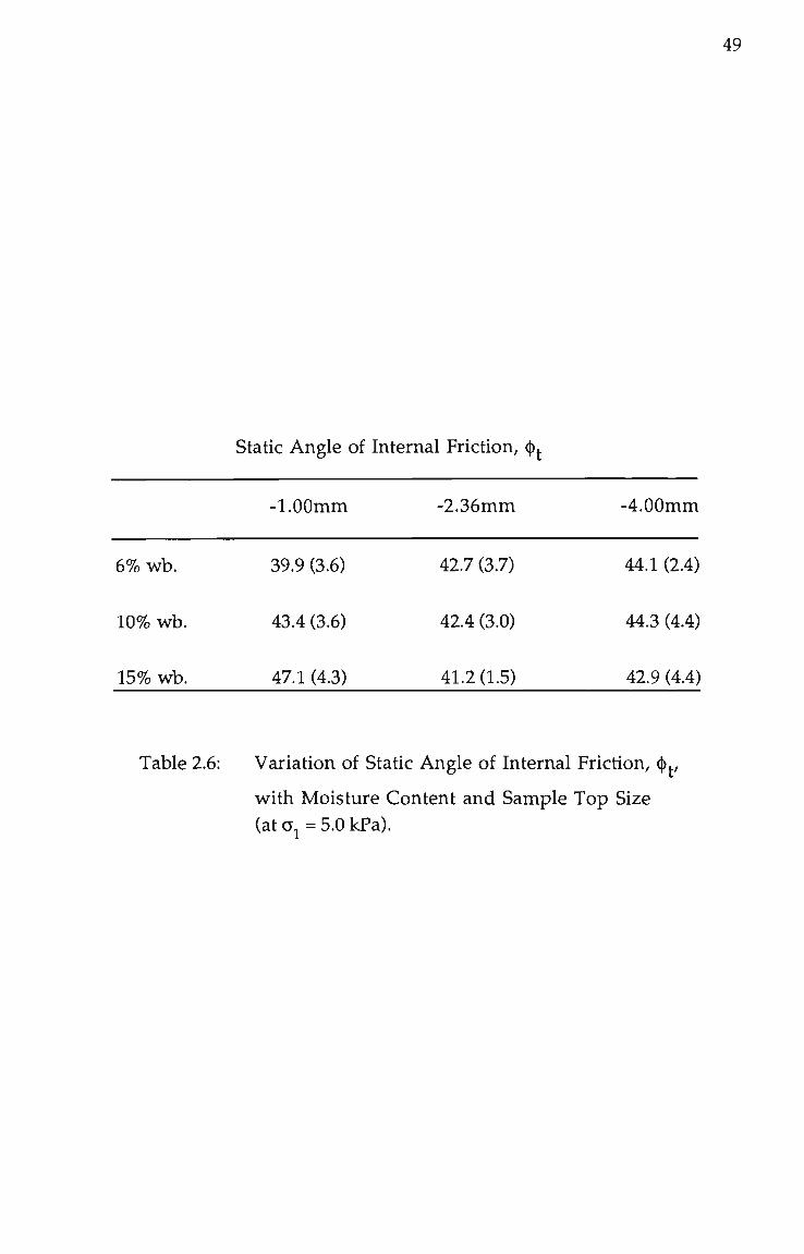
49

Static Angle of Internal Friction, ^.

-1.00mm -2.36mm -4.00mm

6%wb. 39.9(3.6) 42.7(3.7) 44.1(2.4)

10% wb. 43.4(3.6) 42.4(3.0) 44.3(4.4)

15% wb. 47.1(4.3) 41.2(1.5) 42.9(4.4)

Table 2.6: Variation of Static Angle of Internal Friction, ^.,

with Moisture Content and Sample Top Size (at a = 5.0 kPa).

50

The (t)j values listed lie in the 40 - 44 range irrespective of the

particle top size or moisture content, except for the -1.00mm 15% sample.

This particular value indicates the extreme increases in ^^ possible for the

combination of fine particle content and high moisture content.

2.5.4 Wall Yield Locus and the Kinematic Angle of Wall Friction

The wall friction test determines the friction characteristics of the

flow of bulk solids on various wall materials. From the resulting wall yield

locus the kinematic angle of wall friction ^ between the bulk solid and the

wall material, under varying consolidation pressures may be determined.

References [1,21 highlight the importance of the wall yield locus in

ensuring mass flow and slip of the bulk solid along the walls. It is important

that conditions intended for the bin wall should be closely modelled for

testing purposes. Thus the testing of steel samples with a milled surface are

of little benefit since no bin would be lined with a steel with a machined

surface but rather a cold rolled or hot rolled finish. This comment also

applies somewhat to the testing of stainless steel lining plate whose

roughness (as indicated by the R^ value) increases with the sheet gauge for

the same surface finish grade.

Recently there have been several comprehensive studies relating

to wall friction, indicating an appreciation of the importance of this flow

property in mass flow design. Work by Ooms and Roberts [30], ter Borg [31],

and Dau [32] have attempted to quantify the influence of the many variables

acting at the wall material/bulk solid interface. Examples of these factors

include the surface topography of the wall material, relative hardness

between the bulk solid and the wall, and the effects of time consolidation

and extended exposure.

51

The importance of correctly assessing the wall friction for mass

flow design is well illustrated by reports of silo quaking, by Rappen and

Wright [33] and Fang et al. [34]. Silo quaking is the action of a bulk solid

switching between mass flow and funnel flow cyclically on discharge from

bins. This generates extreme vibrations which can not only effect the

performance of the bin but also the structural integrity of the structure. A

suggested reason for silo quaking [33] is the selection of hopper wall slopes

that are to close to the design boundaries of Jenike [3] between mass flow

and funnel flow.

The importance of wall friction will be further discussed in latter

chapters when considering alternative hopper design techniques and the

development of standardised design rationale.

Of the many wall lining materials that are utilised in industry and

that could be considered for testing, the program was restricted to three

different materials, rusty mild steel, 304-2B Stainless Steel (1.5mm gauge)

and Pactene. The reasons for this restricted selection were:

• Too large a number of materials would substantially increase the

testing time and effort for each coal sample considered.

• Experience with coal over a number of years had indicated that

304-2B stainless steel is one of the best performing materials to

line coal bin hoppers [35]. It usually has the lowest friction angles

and has a stable surface finish when left in contact with damp coal

for extended periods of consolidation at rest.

• Rusty mild steel was included due to its common application as a

bin wall material and also because it generally produces the upper

bound on friction angles (comparable to rough concrete).

• Pactene was selected to indicate typical values and trends

representative of the range of Ultra High Molecular Weight

52

(UHMW) polymers that are presently marketed as lining

materials for bin hoppers and transfer chutes.

Microscope photographs of the three wall material samples are

presented in Plate 2.1. The rusty mild steel sample had a typical rough

surface due to rusting, with pits up to 0.3mm deep. The 304-2B stainless

steel and the UHMW Pactene had the standard 'as supplied' surface finish.

As previously mentioned in Chapter 1, for cohesive bulk solids

such as coal, the kinematic angle of wall friction is often not constant, but

varies as a function of the consolidation pressure (due to either a curved

wall yield locus or an adhesion component at zero normal stress) and the

effective angle of internal friction of the j^nrticular sample. Figure 2.6

displays the procedure for determining (J), ulilising the outer intersection

point (representing the arched stress field) between the wall yield locus and

the Mohr stress circle passing through the required consolidation stress a,.

Comparison between wall yield loci provide only superficial

indications since the effect of adhesion, the effective angle of internal

friction and the position of the wall yield locus cannot be accurately

assessed, particularly with regard to values of (|). To provide a direct relation

between ^ and o^ the geometric relations presented in Figure 2.6 have been

solved mathematically and incorporated into a computer program. Chapter

7 presents details of the program which determines the variation of (j) with

a^ and the minimum value of o^ yielding a real solution (ie. when the

Mohrs stress circle of a^ is tangent to the wall yield locus). The subsequent

graphical output, which displays the variation of ^ versus a^ is presented in

Figure 2.7. Comparison of the ^ variations for different wall materials and

coal samples using this presentation is more effective, particularly in the

low stress region which is relevant to mass flow hopper design.

53

(a) Rusty Mild Steel.

(b) 304 - 2B Stainless Steel.

Plate 2.1: (c) Pactene.

Microscope Photographs of Wall Materials Used in Wall Friction Tests (x32 Magnification)

54

Normal Sfress 6, ^

Figure 2.6: Determination of the Kinematic Angle of Wall Friction.

55

60.

50.

40.

30.

20.

70.

60.

50.

40.

30.

20. 1

11

11

:

:

:

"

:

"

:

" 1

\

\

1 . 1 . 1 1 1 . 1 i 1 i 1

i . 1 . 1 . 1 1 1 . 1 . 1

. 1 1 1 1 1

1 1 1 1 1 1

304-2B STRINLE5S STEEL;

:

;

I

, i . 1 . i . 1 . 1 . 1 . 1 . 1 . 1 . =

nUSTY MILD STEEL:

:

i -

1 1 1 1 1 1 1 1 1 1 1 1 1 1 1 i 1 1 1 = 0. 5. 10. 15.

MRJOn CDN50LJDRTIDN STRESS - KILOPRSCRLS 20.

Figure 2.7: Kinematic Angle of Wall Friction Variation.

56

The (]) variations from the testing program are presented in

Figures F.l to F.28. For the two coal samples an additional szimple of -0.5mm

was incorporated into the wall yield locus testing program to further

investigate the influence of particle size. Referring to these figures, the first

apparent feature, particularly for the higher moisture content coal samples

is the variation of <^, reaching quite high values at low o^ values. Thus in

designing for bulk solid flow, for example transfer chutes or mass flow

hoppers (j) values may be substantially greater than those utilised in the

structural design of bins. This fact has recently been emphasised by

Schwedes [36] in discussing the German Din 1055 structural bin design code.

The variation of (^ for each of the wall materials, for the range of

coals tested is presented in Figures F.l to F.6. Concerning rusty mild steel, at

both 10% and 15% the product coals (Westcliff and Coedcliff collieries) have

lower ^ values than the ROM coal samples. There appears to be no other

trend for the range of coal samples tested, the range of ^ for a^ > 4kPa is

approximately 6 . For the 304-2B stainless steel the range of ^ is smaller

particularly for the 10% result, where for o^ > 4kPa, (j) is approximately 18° to

22 . Pactene displays good agreement between the coal samples at 15%

(range of 3 for CT. > 4kPa) but at 10% the results are scattered with a range of

approximately 4 to 6 . There appears to be no major influence of the

increased moisture content from 10% to 15% for ^ values for Pactene.

Figures F.7 and F.8 indicate that air dried coal has a lower wall

friction than the moist coal samples for rusty mild steel (of approximately

3 ). However, for samples with moisture contents in the range of 6% - 15%

similar (j) values were displayed for each wall material. The stainless steel

tends to show the opposite trend, where the wall friction is reduced from

the air dried sample values compared to moist coal. The coal at 6%

moisture content shows a higher friction value than for other moisture

samples (refer to Figures F.9 and F.IO).

57

The ^ variations which are vertically asymptotic to the wall

friction axis for values of CT^ < 1.5kPa indicate severe adhesion tendencies

between the bulk solid and the wall material. This is displayed for the

Westcliff coal (Figure F.9) where the strongest adhesion exists for the 6%

moisture level. This trend is also repeated in Figure F.IO but not to the same

degree.

The Pactene displays a lower wall friction for the air dried and 6%

samples compared to the stainless steel because of the reduced adhesion

tendencies. With increasing the moisture content above these levels the

wall friction of the Pactene increases approximately 3 to 4 above the air

dried values (Figures F.ll and F.12).

The influence of the particle top size on the wall friction for rusty

mild steel, Pactene and stainless steel at 10% and 15% is displayed in Figures

F.13 to F.18. The rusty mild steel results show the -0.5mm sample to have

the higher friction of 32° for both 10% and 15%. Both the -1.00mm and

-2.36mm levels are shown to have similar friction levels but the wall

friction for the -4.00mm sample lies between the variation of the -1.00mm

and the other two particle sizes for both moisture levels. This could indicate

disturbances between the larger coal particles passing over the steel surface.

The Pactene demonstrates a reduction of wall friction with

increasing particle top size. For both the 10% and 15% samples the -0.5mm

sample has (j) values approximately 3 to 4 greater than the -2.36mm,

-4.00mm samples which are similar. The results for the stainless steel are

displayed in Figures F.17 and F.18. The 10% sample <^ variations show

similar ^ values for the particle sizes of -0.5mm, -1.00mm (20°) and

-2.36mm, -4.00mm (17°). The finer samples are approximately 3° greater

than the -2.36mm and -4.00mm samples.

58

Although, at 15% moisture content, the -0.5mm sample again has

the highest friction, the next lower ^ variations occur for the -1.00mm and

-4.00mm samples, the lowest values being for the -2.36mm sample. This

scatter, with a range of some 2 is within experimental error and would

indicate similar (|) values may be determined for the -1.00mm to -4.00mm

sample range, particularly at higher CT^ values for the stainless steel.

Table 2.7 (an excerpt of Table 2.2) displays the variation of <^ for

304-2B stainless steel for CT^ = 5.0 and 7.5 kPa, for a combination of particle

top sizes and moisture contents. Only the stainless steel results are repeated

because of its common application as a hopper wall liner. Bracketed figures

refer to the standard deviation. The table indicates that for the -2.36mm and

-4.00mm samples (J) is essentially constant for the various moisture contents

when CT^ > S.OkPa. The -1.00mm values for CT^ = 5.0 and 7.5kPa show

substantially greater ^ values than determined for the other samples

(particularly at 6% and 10% moisture contents) because of increased

adhesion of the coal to the wall surface.

2.5.5 Bulk Density Variation

For the design of storage bins the variation of bulk density with

increasing consolidation stress is required. The lower values are required

for the determination of hopper outlet dimensions and feeder loads, while

high values of stress are used when predicting bin wall pressures.

The results from the Jenike Compressibility Tester may be

represented conveniently by the power equation:

CT, 1^

P = Po(—) ;<Ji>0 (2.2)

where

p = solids bulk density corresponding to the major consolidation

stress CTj.

59

Kinematic Angle of Wall Friction, (j), for 304-2B Stainless Steel

Sample -1.00mm -2.36mm -4.00mm

5.0kPa 7.5kPa S.OkPa 7.5kPa 5.0kPa 7.5kPa

Air Dried 22.6(0.9) 21.7(0.8) 22.1(4.1) 21.5(3.9) 20.5(0.7) 19.9(0.6)

6%wb 29.7(3.4) 25.8(2.4) 22.4(2.4) 20.2(1.5) 21.2(1.6) 19.3(1.3)

10% wb 25.1(1.0) 22.2(0.8) 20.4(1.3) 18.7(0.9) 19.3(1.4) 18.0(1.3)

15%wb 23.8(2.0) 21.3(1.8) 20.2(1.4) 18.6(1.0) 19.5(1.9) 17.9(1.3)

Table 2.7: Variation of Kinematic Angle of Wall Friction, (]), for 304-2B Stainless Steel, with Moisture Content and Sample Top Size (at CT^ = 5.0 kPa).

60

p = solids bulk density corresponding to the arbitrary major

consolidation stress CT^. (The respective values of p^ and CT^ are

normally selected as the centroid of the experimental data as

determined from the statistical curve fitting procedure.)

b = compressibility constant for the particular bulk solid.

Thus, for any bulk solid, values of CT^, p^ and 'b' are required. By

plotting the above variation on logarithmic axes it is apparent that 'b' is the

gradient of the resulting straight line and is a measure of the compressibility

of the bulk solid. The testing program results indicate that the variation of

bulk density with consolidation pressure is accurately modelled by the

above equation. Utilisation of this equation allows a more consistent

appraisal of bulk density under different loading states. Other researchers

[37] have used terms such as tapped, aerated, lightly packed etc. which

involve disadvantages in determining when to apply the various terms and

does not allow the variation with consolidating stress to be appreciated [38].

A summary of the experimental bulk density variations is

presented in Figures G.l to G.14. These figures present the bulk density

variations derived from the power equation form, curve-fitted to the

experimental data.

The following trends are apparent from a comparison of the

results:

For the collieries of the Illawarra region, the range of bulk density 3 3

is 150 - 200 kg/m about mean values of approximately 800 kg/m 3

for 10% samples and 900 kg/m for 15% moisture content samples

(CT = 7.5 kPa, Figures G.l and G.2). This range is significant since

for many of the collieries, coal is mined from the same seams

using similar extraction methods. The maximum bulk density

values (at higher consolidation stresses CT^: 50 < CT^ < 75 kPa) for

61

3 3

10% samples are 1000 kg/m and approximately 1050 - 1075 kg/m

for 15% coal.

• The bulk density generally increases with sample top size for coal

at the same moisture content. As an example Figures G.3 and G.4

display the bulk density variation of Westcliff Product coal at 10%

and 15%. As depicted the -2.36mm and -4.00mm samples produce

the maximum values. An overall analysis of Table 2.2 indicates

the -4.00mm samples have bulk density values 10 - 12% greater

than the -1.00mm sample at 10% and 5 - 6% greater at 15%

moisture content (based on CT^ = 7.5 kPa).

• The bulk density variation with moisture content for samples of

the same particle top size is presented in Figure G.5 to G.8. In the

range of CT^: 5 < CT^ < 15 kPa the bulk density for air dried coal is

higher than moist coal at 6% and 10% and approximately the

same order as the 15% samples.

• The air dried samples usually represent the least compressible

state Cb' values of the order of 0.02) compared to those of higher

moisture contents. The variation of 'b' is significantly affected by

the sample moisture content. The values of 'b' increase from the

air dried condition values to a maximum which is often at the

10% level and reduces for the 15% test sample.

Table 2.8 provides a summary of the variation of 'b' with

moisture content for the -2.36mm coal samples.

2.6 COMPARISON OF THE FLOW PROPERTIES FOR THREE COALS

WITH SIMILAR PARTICLE DISTRIBUTIONS.

This flow property testing program was instigated to highlight

differences that might occur for test samples having similar particle

distributions at similar moisture contents (maximum moisture content

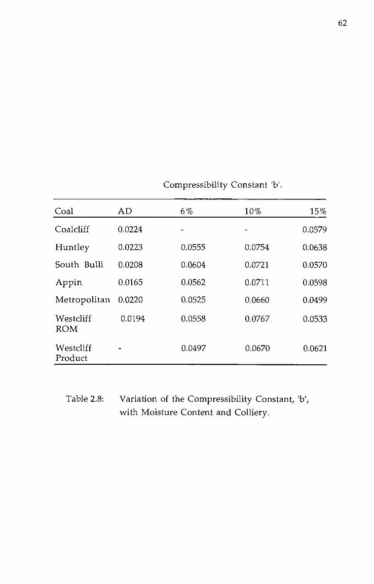
62

Compressibility Constant 'b'.

Coal

Coalcliff

Huntley

South Bulli

Appin

Metropolitan

WestcHff

AD

0.0224

0.0223

0.0208

0.0165

0.0220

0.0194

6%

-

0.0555

0.0604

0.0562

0.0525

0.0558

10%

-

0.0754

0.0721

0.0711

0.0660

0.0767

15%

0.0579

0.0638

0.0570

0.0598

0.0499

0.0533 ROM

Westcliff Product

0.0497 0.0670 0.0621

Table 2.8: Variation of the Compressibility Constant, 'b',

with Moisture Content and Colliery.

63

difference between samples was 0.5% wb). The three coal samples were

Westcliff ROM, Westcliff Product coal and a Queensland Product coal.

Elimination of the influences of particle distribution and moisture content

from the results ensured that any differences in the flow property results

largely would be due to a combination of the following factors:

the effect of washed coal product compared to ROM coal samples

differences in the coal from the two coalfields

differences in the ash constituents

differences in the maceral content ratios

particle shape

traces of washing mediums retained within samples

The samples used came from two coal basins featuring different

characteristics. The Westcliff ROM and Product coal was mined from the

Bulli seam, within the Sydney Basin and represents a hard coal (H.G.I, of 56)

with a low inherent ash content. The second sample came from the central

region of the Bowen Basin of Queensland and represents a very soft and

friable coal (H.G.I, of 87).

Samples were prepared as -2.36mm test samples and the flow

properties assessed at 10% and 15% moisture contents, representing typical

values at which the coal is handled. Figures C.23 and C.24 compare the

instantaneous and 3 day time flow functions of each sample. At 10% the

Westcliff ROM and Product coals have similar instantaneous and time flow

functions. The Queensland sample displays substantially stronger flow

functions particularly for the time storage conditions (approximately 0.7 kPa

above the Westcliff coal samples). At 15% the increase of the time flow

function above the instantaneous is greater compared to the 10% samples,

typical increases being 0.8 to 1.8kPa for the range of the displayed flow

factors. Figure C.24 also displays the positioning of the instantaneous and

64

time flow functions into two distinct groups, the stronger time flow

functions occurring for the Westcliff Product and Queensland Product

Coals.

Comparison of the flow functions with results from other

testwork (refer Figure C.21 and C.22) indicate that they are typical of the flow

functions determined from other testwork where the sample particle

distribution and moisture content was not as closely controlled. These

figures indicate the Queensland Product coal to be in the stronger range of

the coals tested.

The effective angle of internal friction results displayed in Figure

D.9 shows similar trends and values, determined from other flow property

testing. The results of the Westcliff ROM and Product coals are similar, with

typical values of 60 for 10% and 68 (CT = 5kPa) for 15% moisture contents.

The Queensland coal however displays similar values for both moisture

contents of approximately 5 = 66 . For all the samples at 15%, there was a

marked decreasing variation of 5 with increasing Oy typically 70° to 55° for

CT^: 0 < CTj < 20kPa. The (|)j results (Figure E.7) display a similar level of scatter

that was found for the other coal sample tests. However, the Westcliff ROM

coal samples indicate similar results ^^ ~ 48 for both 10% and 15% moisture

contents. The Queensland and Westcliff Product coal samples displayed

lower values of ^^ of approximately 42 - 46 .

The kinematic angle of wall friction results are displayed in

Figures F.19, F.20 and F.21 for rusty mild steel, 304-2B stainless steel and

Pactene respectively. Generally the results followed similar trends to those

displayed from other testwork in regard to moisture content and type of

wall material. For each wall material ^ values were found to be within a 4°

range independent of the moisture content. Average values for (j) were

found to be 27 - 28° for rusty mild steel, 18° - 20° for stainless steel and 23°

65

Pactene (CTJ = 7.5 kPa). For two samples, Westcliff ROM (15% moisture

content) and Queensland (15% moisture content) the ^ variation for

stainless steel was quite different to the general trend of values noted. The

Westcliff ROM was substantially higher (20° <^< 25°), and the Queensland

coal below the average ((]): 14 <^<ll ).

The bulk density variations for coal samples at 10% and 15%

moisture contents are displayed in Figure G.9 and G.IO respectively. They

display approximately the same form for each sample indicating equivalent

values of 'b', the compressibility constant. The results indicate in relative

order of decreasing bulk density to be Queensland, Westcliff ROM and

Westcliff Product. The bulk density values are also shown to increase 12 -

15% with a moisture content increase from 10% to 15% wb.

Overall the flow properties determined for the three coal samples

are typically within the range of values found for similar moisture content

coal samples. The Queensland coal sample did indicate stronger flow

functions (particularly at 10%) and higher bulk density values, but for the 6,

(|) and ({) flow properties there were no definite trends. Comparing the

Westcliff ROM and Product samples, similar flow properties were found

between both samples^ although the Product coal displayed a stronger time

flow function at 15%.

2.7 INFLUENCE OF PARTICLE SHAPE ON FLOW PROPERTIES.

To assess the changes that can occur in the shape of coal particles

from handling operations and to investigate the subsequent effect on the

various flow properties a sample of Westcliff ROM coal was tumbled in a

Friability Drum Tumbler constructed according to ASTM D441 - 45 [39]. The

Friability Drum Tumbler simulates coal degradation (such as occurs at

transfer points) and allows the determination of a Friability Index for

comparison with other coals.

66

Examination of the samples after tumbling indicates rounding of

particles greater than 4.00mm occurred but generally little rounding

occurred for the finer particles. Plate 2.2 presents SEM photographs of coal

before and after tumbling and indicates that brittle fracture of particles

occurred in preference to rounding.

Two samples of Westcliff ROM coal were prepared for flow

property testing, one as a -2.36mm control sample and the second, which

after tumbling was remixed to the same particle distribution as the control

sample. Flow property tests were conducted at 10% and 15% moisture

content. Figure C.20 displays the instantaneous and time flow functions of

both samples. The tumbled coal is shown to have stronger flow functions

(compared to the control sample) however within the range of the

displayed flow factors the relative differences are small. The other flow

properties of effective angle of internal friction, static angle of friction,

kinematic angle of wall friction and bulk density variation indicate similar

values to those found from other coal testwork. Figure D.IO shows a typical

decreasing trend of 8 with increasing CT^ with comparable values occurring

for both moisture contents, typically, 8 = 60 (for CT^ = 5.0kPa) with a range of

4°. The variation of (1) with CT^ is presented in Figure E.8 and shows the

tumbled coal sample to have higher values above the control sample

(typically 4° - 5° ) at both moisture contents. For CT^ = 5.0kPa, the tumbled coal

(l)j. was approximately 42 compared to 37 - 38 for the control sample. At

15% both coal samples displayed an increasing trend of (j)j. with increasing CTH

whereas relatively constant values occurred for the 10% sample.

The variation of (j) for Pactene and 304-2B stainless steel is

presented in Figure F.22 for the tumbled and control samples at both

moisture contents. The characteristic friction values found from other coal

tests of 22° for Pactene and 18° for stainless steel are indicated. Comparison

between the control and tumbled samples indicate no definite trends with (()

67

^ ^ ^ ^ v *

. ^p r

ili J^' • " ^ ^ • - '

(a) Conti-ol Sample, 125 x 150 i^m.

^^^^^ ^ ' ^*V^^B^^^M v^^^l^^^^^^ft

(b) Tumbled Sample , 125 x 150 |j.m.

Plate 2.2: SEM Photographs of Westcliff ROM Coal,

Control and Tumbled Samples (x250)

68

values being within a 3° range for CT^ = 5kPa. Figure G.ll displays the bulk

density variations for the tumbled and control samples. The 15% tumbled 3

sample is shown to be approximately 50kg/m greater than the control 3

sample. Typical asymptotic values for the samples are 1020 kg /m , 970

kg/m^ and 940 kg/m^ for the 15% tumbled, 15% control and 10% tumbled

samples respectively. The typical increasing trend of bulk density with

increasing moisture content is displayed. Reference to Figure G.15, in

providing an overall comparison of the bulk density variations for

Westcliff coal indicates that the tumbled sample is typical of the results

determined from other tests.

The effect of the sharp angular particles is shown to have only a

minor effect on the coal flow properties when comparing the results from

the control sample and from other test results. The results show no definite

trends that could be attributed to the particle shape. The tumbling operation

indicated that coal particles could be expected to generate sharp angular coal

fines by brittle fragmentation in preference to abrasion and rounding the

coal particles from repeated handling operations.

2.8 FLOW PROPERTIES OF SAMPLES OF FREE CLAY MIXED WITH

COAL.

This testing program was instigated to assess the effect of clay

mixed with coal samples on the various flow properties in simulating the

storage and handling characteristics of high ash content coals. Preparation of

the test samples were based on Westcliff ROM coal which was air dried,

sieved to -4.00mm and divided into four samples of approximately the

same particle distribution. Flow property tests were conducted on two clay

types. Kaolin, a non-swelling clay and a swelling day Bentonite.

Commercial grade Kaolin and Bentonite was added respectively

to two samples to increase the ash content from approximately 11% to a

69

nominal 25%. To the third sample a similar amount of coal fines (-45 |im)

was added to indicate the relative effect of the added small particles

independent of the chemical effects of the clay. The fourth sample was

retained as a control sample to provide a basis for the flow property

comparisons.

The physical appearance of the resulting test samples are

presented in Plates 2.3 and 2.4 which display SEM photographs of the

control and coal with Kaolin samples at two magnifications. The graded

particle distribution of the coal particles with typical sharp edges and

conchoidal fracture planes contrasts with the appearance of the coal particles

embedded in a matrix of clay platelets for the Kaolin and Bentonite samples.

The instantaneous and 3 day time flow functions from the test

program are presented in Figures C.27 to C.30. At 5% the flow functions of

the clay samples are comparable to the coal plus fines sample. The time flow

functions display only a small increase over the instantaneous condition,

which was expected for this low moisture content. For 10% moisture

content the two clay samples and the control sample had similar

instantaneous flow functions with typical values of CT : 1.2 < CT < 2.5kPa

within the displayed flow factor range while the coal plus fines sample was

significantly higher with CT^ values in the range of 3.7 - 4.5 kPa. Comparison

of the 3 day time flow functions for the clay samples indicate the high

values of CT^^ attainable which are approximately double the instantaneous

values.

With increasing moisture contents, the unconfined yield strength

continues to increase. For the Kaolin day sample this increase was such that

shear tests were conducted only to a maximum moisture content value of

12.5% due to the strong instantaneous flow functions. The time flow

functions for the clay samples at the higher moisture contents indicated the

occurrence of a cementing action or 'set' which was relatively insensitive to

70


(b) Coal Mixed with Kaolin Sample (x285).

Plate 2.3: SEM Photographs of Westcliff ROM Coal

(Control Sample) and Coal Mixed with KaoUn.

71


(b) Coal Mixed with Kaolin Sample (x2880).

Plate 2.4: SEM Photographs of Westcliff ROM Coal

(Control Sample) and Coal Mixed with Kaolin.

72

the values of Oy The time flow function for 15% Bentonite depicted in

Figure C.29 was typical of this action. Figure C.28 displays the time flow

functions of the coal plus fines sample leading to comparatively high CT^^

values with steeply sloping flow functions. Again the CT^^ values determined

for the coal plus fines samples were approximately double those values

found for the control sample.

An overall comparison of the flow functions indicates that the

clay samples have similar instantaneous flow functions to the control

sample up to moisture contents of 10%. Above this level the clay and the

coal plus fines samples have similar values which are significantly stronger

than the control sample results. Concerning the time flow functions, above

10% moisture content both clay samples displayed extremely strong levels

of unconfined yield strengths typically caused by a cementing action. In

several instances the clay sample time flow functions were similar to those

determined for the coal plus fines samples.

Mikka and Smithan [10] who also tested the influence of Kaolin

and Bentonite on the handleability of coal (but for a lower ash content %)

found that the non-swelling clay had little influence. However for the

swelling clay, Bentonite, handleability deteriorated rapidly above 8%. On

this basis, they correctly highlight the significance of the actual clay mineral

(for instance Scott and Graham [40] report on the handling problem, coal

mixed with montmorillonite) and not just the actual level of clay present.

Considering the effective angle of internal friction. Figure D.ll

and D.12 present the results of the four test samples. At 5% moisture

content, the clay and coal plus fines samples display similar 8 variations

ranging typically from 58° to 52° for CT^: 0 < CT^ < 20kPa. At the higher

moisture contents a greater variation is indicated (Figure D.12). The control

and coal plus fines samples display similar 8 variations which were typical

of the values from other moist coal testwork. Comparing the clay samples.

73

the Bentonite sample displayed constant values of 51 and 55 for moisture

contents of 10% and 15% respectively, which were unusually low for such

coal samples. The Kaolin sample at 10% displayed a constant value of 8 =

60°, but at 12.5% displayed significantiy higher values ranging from 76° to

62° decreasing with increasing CT^.

Referring to the ^^ results, comparison between Figures E.9, E.IO

and E.4 (displaying (j). results from other coal testwork) indicate similar

values and ranges. Figure E.IO indicates that most ^^ results for the four

samples gave values in the range of 40 - 48 . There appears to be no definite

trend, although the lowest (t) values occurred for the control and coal plus

fines 15% samples and the maximum values occurred for the Kaolin clay

samples at 10% and 12% moisture contents.

The results of the kinematic angles of wall friction for the three

wall materials, rusty mild steel, 304-2B stainless steel and Pactene are

presented in Figures F.23 to F.28. Comparing the values for the coal plus

fines and control sample, the moisture content is shown to have the

greatest effect compared to the effect of the fines content difference between

the two samples.

For example, Figure F.24 shows that for stainless steely the 15%

sample has df values 2° - 3 less than the typical 10% values of 18 - 17 . The

day samples of Kaolin and Bentonite have reduced ^ values compared to

those of the control and coal plus fines samples. This is best displayed by

rusty mild steel (Figure F.26) and stainless steel (Figure F.27). For the rusty

mild steel typical ^ values from the clay samples (at both 10% and 15%) are

approximately 26° compared to the higher values of 30° - 27° for the coal

plus fines samples. Figure F.27 for stainless steel displays lower values

typically of 15° (particularly for the Bentonite) compared to values ranging

from 20° - 18° for the coal plus fines samples. The wall friction values for

74

Pactene display little variation for the different samples and moisture

contents, with (j) values typically being 22° with a 2 range for CTJ > 5.0kPa.

The clay samples displayed values of bulk density that were 10% -

15% above the control and coal plus fines results, which was expected due to

the higher specific gravity of the clay. Figure G.13 displays the bulk density

variations at 10% moisture content where the relative order of samples in 3 3

decreasing bulk density was Bentonite (1080kg/m ), Kaolin (lOlOkg/m ), 3

and the coal plus fines (960kg/m ) and control samples being similar. The

four bulk density variations displayed have similar variation curves

indicating similar 'b' or compressibility constants. The results for the 15%

moisture content (Figure G.14) display increased values relative to the 10% 3

results, with the maximum Bentonite value of 1150kg/m . There is also a

discernible difference between the control and coal plus fines samples of 3

approximately 30kg/m , the coal plus fines variation being the higher

result.

Generally^ the flow properties of the clay samples are similar to the

coal plus fines samples, and indicate reduced handleability compared to the

control sample. The most apparent and critical feature of the day samples is

the high cohesive strength displayed by the flow functions for moisture

contents in excess of 10%. This is especially prominent when considering

the time storage of coals with these characteristics where a strong 'set' or

cementing action can occur. Concerning the other flow properties, the 8 and

<t)j variations were generally similar to the results found from other

testwork, however the clay samples displayed reduced (]) values for some

wall materials and significantiy higher bulk density values compared to the

control and coal plus fines samples.

75


The investigations reported in this chapter have concentrated on

the flow properties of samples of hard black coal from the Southern

Coalfields of the Sydney Basin and to a lesser degree the Bowen Basin of

south eastern Queensland. The influence of sample variables such as

moisture content, particle top size of sample, particle distribution and time

consolidation at rest on the various flow properties has been investigated.

Assessment of the various parameter influences is on the basis of

the Jenike shear cell tests. This approach has been reported (Mikka and

Smithan [10]) as displaying reduced sensitivity in differentiating between

the general handleability of coals. This instance is illustrated by coals that

contain varying levels of fines in the full size distribution but yield similar

flow property results because the test samples have similar 0 x 4mm particle

distributions. Utilising the flow properties determined from the shear tests

is justified however, as this study is concerned with the design of storage

bins.

The most influential parameters were found to be the sample

moisture content, values from Air Dried (generally 1 to 2.5%) to 15%wb.

being considered, and the sample cut size, as represented by the particle top

size of the test samples. The combined effects of moisture content and

particle distribution are displayed in Figures 2.8, 2.9 and 2.10 where the

variation of the unconfined yield strength (represented by the flow

function) with moisture content is presented. This flow property is crucial

to the determination of the critical outlet dimension in mass flow hopper

design. The variation of CT with moisture content is apparent, from the

characteristics of a simple bulk solid occurring at air dried conditions to

maximum strength occurring for moisture contents in the range of 10% -

15%, typically the moisture levels in the fines fraction at which coal is

transported and stored. The effect of the increased fines content is depicted

76

'^dH-^P SS3yiS QIHIA OBNIdNODNn

Figure 2.8: Variation of the Instantaneous Flow Function

with Moisture Content Based on -1.00mm test

sample (Mean Values Displayed).

77

Bd>l ^P SS3biS ai3IA QBNIdNQDNn


with Moisture Content Based on -2.36mm Test

Sample (Mean Values Displayed).

78

^d^-^P SS3biS 013IA QBNIrlNODNn


with Moisture Content Based on -4.00mm Test

Sample (Mean Values Displayed).

79

in Figure 2.8 where at high moisture contents CT developed may be double

the values determined for the two larger particle cut test samples.

Comparison between Figure 2.9 and 2.10 present similar results and indicate

that the -2.36mm sample does not necessarily lead to conservative flow

function results compared to the -4.00mm sample.

A summary of the mean flow property values from the testwork

has been presented in Table 2.2 and for the -2.36mm test sample graphically

displayed in Figure 2.11. The effect of time consolidation at rest in leading to

significant increases in the unconfined yield strength above instantaneous

conditions is apparent. The difference between CT^^ and CT increases with

increasing fines content and moisture content of the sample.

The effective angle of internal friction develops two trends with

increasing moisture content, the value of 8 increases and a marked

variation of decreasing 8 with increasing CTJ (for CT^: 0 < CT^ < 15 kPa) occurs.

At 15%, typical 8 values range from 60 - 70 . The static angle of internal

friction displayed the least identifiable trends of the flow properties

considered, with ^^. values ranging from 40 - 45 for moisture contents of

10% and 15%.

An important aspect involved in the design of mass flow hoppers

and transfer chutes is the wall friction value and variation typical of wall

lining materials for various physical conditions of the coal (moisture

content and particle size distribution). Each wall material has a characteristic

(j) value range which varies according to the moisture content and to a lesser

extent the particle size distribution. An important feature, particularly

regarding the performance of smooth metal lining materials (eg. 304-2B

stainless steel) with moist coals is the action of adhesion, and for other wall

materials, convex upward wall yield loci which lead to variable cmgles of

wall friction dependent on CT^. Figure 2.11 displays the typically high values

of (]) which can be developed for 304-2B stainless steel at low CT^ levels.

80

1000

.E 900

s-I

O H

iZ flOO

^ 700

30

3,." u. a o I UJ ^

iaz 20 z o

ii z

AIR DRICD

WAU HAURIAL 30I.-JB SIAINUSS S U t l

2-5 50 7-5 MAJOR CONSOLIDATION STRESS d^-kPa

Figure 2.11: Typical Variation with Moisture Content of the

Flow Properties Required for Mass Flow Hopper

Design (Mean Values from -2.36mm Sample

Tests Displayed).

81

The bulk density variation leads to asymptotic p values for high

CTH values. Generally, the maximum p values occurred for the air dried and

15% moisture content samples. The bulk density values decreased from

these levels for moisture contents of 10% and 6%.

Other testwork considered the influence of particle shape, and the

addition of clay to coal test samples to simulate high ash content coals.

Comparison of the flow properties of tumbled coal with a control sample

indicate minor influences due to the particle shape. SEM photographs

indicated that for repeated handling operations the coal particles would

tend to remain angular and fragmented in nature due to brittle

fragmentation which occurs in preference to an abrasive and rounding

action.

In simulating high ash coals, the flow property testing of coal

samples mixed with two clay types (Kaolin and Bentonite) indicate similar

flow properties (particularly the instantaneous flow function) to those that

would be expected for high fines content coals. Although the clay samples

displayed reduced (j) values for some wall materials compared to the control

sample, the major feature was the extremely strong time flow functions

which occurred for moisture contents above 10%. Several of these time flow

functions displayed a 'cementing' action where the variation of CT^ was only

slightly influenced by CT^. These results are pertinent to those coals

containing certain clays. Several researchers [11,40] comment that these

coals present no handling problems immediately after mining and when

relatively dry. However, when the coal is exposed to the weather for periods

of time, moisture is absorbed and the coal degrades, with the clay

component forming a sticky matrix.

82

CHAPTER 3

SENSITIVITY OF IVIASS FLOW HOPPER GEOMETRY

PARAIVIETERS TO COAL FLOW PROPERTIES

3.1 INTRODUCTION

The mass flow critical hopper geometry parameters have been

determined for the coal samples whose flow properties were tested and

reported in the previous chapter. Review of the hopper geometry parameter

values provides a tangible indication of the influence of the various flow

property trends, and gives an overall appreciation of the effect of such

variables as sample moisture content, particle top size and time

consolidation at rest can have on the design of mass flow storage bins.

The critical hopper geometry consisting of hopper wall slope, a,

and outlet dimension, B, for axisymmetric and plane flow hoppers has been

determined for both instantaneous and time conditions for the wall lining

materials of rusty mild steel, 304-2B stainless steel and Pactene. The

calculation of these parameter values was achieved by a computer program

utilising the Jenike method [3, 4] and described briefly in Chapter 1.

The values of the critical hopper geometry parameters are

presented in tabular form in Tables H.l to H.21. Table 3.1 presents a

summary of the critical hopper geometry parameters for all the coal sample

tests except for those of the free clay testing program. For each category two

values are presented, the first being the mean and the second bracketed

value, the standard deviation of the data set. Note, that the mean and

standard deviation for each category has been calculated on data sets with

different numbers of results.

83

OJ

"B. fQ

V) * j

tn .OJ H 6

.OO

mj

T

01

Sam

p]

4-. trt

E2

B

CM 1

OJ

7! B

U3 - U i

tn

F

e B

•1.0

0

'

^

1 B

in G

eom

e V c 01 1J a

^ CO CM

t o

"S.

1

V § u

tn i n

CQ CM

CO

V)

OJ c SI u D>

l« CQ CM

CO

a i r 3 K

10

4-»

s )-l

- M

s 6 o CJ 01 u

s tn

o 1 V O

G CM

CO oi

^ • ^

r ^

CM s..*

O

!» r-<

.— OS d '..'

m • ^

5 CM

»-*'

°1 OS

'-'

-... Ot) iri •.^

r-. i r i

to r H

vq CM

1^

CM CO

1

O Tji

9' o

<^ CM

..• bb u 3 >

R N

i n OS r H

... r H

CM

o OS r H

.—V

OS O

tD

tri

t o CM

SO 13 fS

R i n

^ tri r H

r-. r H

r H

T(i

^ iri

K

r H

1

i n

rs

5 d '

oo CO

. ^ 1 .

bb 3

«"

r-; CO

CO OS CM

.-.* t n rM

CO

K t s

,«, OS

d

o r H

CO CO

vD CD CO

...... SO OS S w '

t s d cs

CO r- s * - .

H CM I - H

00 OS

00

a

o d f.*

so CO

^~^

t ^ OS

. bb 3

So rsi

r^ d CO

^H« .

t o (S

oo DC) CM

- o> d

i n

r H

Os' CM

• ^

f..

CO

^ . v

C3 VO

•* CM

r-; r H

SO CO

'"'

P SO

o

CM

I

o t s r H

CM CO

"—'

N r-J r H

.- bb 3

O f - H

S3

t s r H

s R t s

i n K

R

^..^ 00 f.^

VO Ci

t s r-< r H t o

OO r- t s r H

^ O t>;

«

,- Os vd ' r - t * • * '

t ^ r H CT> SO

vO

-* CO

"^ o OS

s R OS • . *

r H

t s

^

1

a !Q

s 1

1

,- g ^

^ i n m CO

t s so

fe ^.^ t n r- CO o

i n CM so 00

(^. tri c^ CM

O

S

i n

cs

s i n t s

^

.. i n CM i n CM

00

8 00

i n CO i n r-«

^^ O

d OS so

R iri

a o d 00

q 00 OS r H

O

d CM 00

t n • *

OS

i n t <

- B ^ ca

R 3 r-f

t s SO 00 CM

.. SO

d r H

i n CM s o CO

- • ^

s O

3 CM

q SO t s

q CO r H CO

,.. .—* iri oo

q r H O CO

OS SO

O t s 00 CM

CM OS i n

n CM

VO

d r H

i n

f:: CM

R t>:

s

o d tn t s

. - . V

B J

CM

iri so r H

q d cs CO

^^ T-*

•* r H

O

d

. r H

rsi t n f - H

o tri CM

P •* o r H

^ i n t^; s o CO

^ - v

CM

d 00

t ^

OO CO

00 r H

OO

oq ot) t n t o

cs oti o r-.

*—' q

1 so

rs o t-*

^"^ t n ts' r H

i n 01}

21

o

CO

o B J

CQ pQ

S g 0)

5 o

o t—i

q cs

•* OC) r H

^ r H

•*

OS

d CM

R r H

t n 00

P CO

Os t ^ r H

^ p . . .

<3S 7-t S . *

q r-. CM

q r H

i n

tri

Os' T-t

o

f 1 S£i

r H

SO

.—.

VO t o

Os

iri

^^ bb 01

3 8 "

t o CM

t s OS r H

^ - v

°9 rM

CM • *

CM

/ - S

OS r H N . ^

t s 00

R r-< S . * '

""t ON r-*

^^ r^ 1—<

CO

a oc> r-i

CM t s

R r H

<Js I s

n r - i

SO d cs

R t o

o t - ;

^ bb 3

t! a

q CM

tjs 013 CM

, Csj tri

so

d CO

^.^ ejs f ~ .

• *

00

VO CO

OS t s CM

,_ i n CM

CO

d CO

q r-i

O

tri r.1

CM CM

._ t < CS

5£

r-.

tri CM

Co CO

• *

iri

^^ bb

3

Os' q

rsi so

" a CO tr^ d CM CO g

r H

. — s ^ ^

O so CO CS s-> •»!•

t s

O 00

iri oo CO g

r H

^ s ^ s t s CM CS r-*

^— o CM

t n o

S 3 OS

P q r-i T)!

- a O rH

d rM CO g

r . .

. - s .—. r H OS

r-! CM w i n

t s

so O

S R o

00 00

r-I tri s - ' r H

d

t s CO so 00 r H r H

OS

0 0 r H

r-i rsi •^ CO

s IT) C^

0 0 SO

r H

r H OS

rs i OS —^ OS

s: o o d d CO i n

CO VO

•* tri •-!- t s

t o

OO q so d r-* t s

rM r H

. * s ^ ^

bb c 3 S

s ' ^ t ^ w "

R d OS O

t s

1 r H

. H N

to CS O •<t" v >

t s

IT) r H

R iri i n G

t o CO OS rM

R OS • *

CM

o so

S '-' .. t s t s • *

CM

o

3 m

i n

t>: 00 r H

O

d 00 CM

in Tfi r H

CS

00

1 rM

csj

rsi to CM

o d r H r H rM

cs d r H rM

n

, - v

B g CO

n 00 o r H

q iri 5

/ • ^

n •* <5S S ^ '

O

d 5 ,m^

CH

s t^

§

R t < r H r-i

r-. rM

S

,* ON

CO

r-<

**-' tn OS

00 t < o r-t

rM OS

^

so CTs O t s

q iri

n •te

a n r-<

s oo m OS r H

n 1

^ s 5

S VO oo I - H

tv. r H

0 \ SO

^ CS OC) 00 r.* s ^

i n

id R

R tri t s

n ro

R t s O r H N ^

o Os

s R • *

o r H

s.-

o

^ t s

CO t-; Os s ^

q tri 3

CO p - t

CM r-<

'.- 00

i Os

00

er> CM v. . -

^ i n Os

R OS O

'^ "? <Js OO

.- B sg

CQ CO

1 § U 0)

to

•3

to t - H

R r H s . ^

r H

t s r H

, c^ rM

•* a ^«.. i n CM

n in

00

d v^

SO N: r H

. •W

. s.^

SO

a q fi s ^

tjs SO

CO CO o

oo CO

fH m -

o oi r H

R cs s j -

o so

•a

a"

d

o Os r.*

^ s

• * .

r H S v .

t n

•* cs

..- • *

rsi

n t s

q r H • w .

i n 00 r H

. •* T-H

t s

a CO CO s . '

fS t s

R d

^ t s I-H

r-<

..

• ^

?i

R r>i

m t s

.~^ bb u 3 «

OS r H

.., t>: CM

R «i s.«

so rsi CO

.-s O

^

00 • ^

OS

d

t s t s CM

^ s 00

^ s . ^

Os

CO

CM rf)

m so

CO

• o

„ a

n so s.*

a oa CM

® CS s-J

so

tri r H

^ bb

3

*—s / - S i n so d t j i s- ' t n

Ci

so c<5 OS r H

CM g r-*

' - s ^ OS 0 0

<-^ c i N ^ 0 0

ts s . .

. * Ct)

tri so CO ^

r—

.—s . " ^ T) ; OS

rsi 3! S H ^

CJ

0(3 P^

r-t r-t

o so r-i oi

^ a S w .

°° t^l 0 0 OS CM CO

r-t

^ - s ^ - s OS i n ri CTs - ^ t o

rM S H "

i n Ti;

S o CM

i n OS rtj otj s ^ r-i

JM

00 t s

so iri rH rM

r-t

00 R d CO — CO

i n

H* O

CO r H

rM • *

ci K i n

CO q rM r-i

r-t

O CO CO • *

- g r H O

l-H SO CM r-t

^ N ^ „ ^

bb c 3 H

a a »

r H

tri 00 i n ,

OS

m r t

. H . . r H

d rM so

n r - '

3 r-t

^.. rM so t s i n

o d c^ CO r.*

SO

rsi o CO

n i n

9 r H

- t o • ^

r-" CO •yJ'

•o

s i n r H

o

«* o^ CM.

i n t s 00 t s r - i

CM

SS *-^ o

r H

rM

ro •.ji t n s ^ .

o d r H

a R so rM r H S . '

n oo r H

. - V

B g

ti CO

R d ro r H

OC) CO

9

f> NO 00 ro r H

^•^ i n

i n

*r j • ^

!S ( N | r - H

t o

^

• ^

00 r-t r-t

• ^

O

d i n i n

..-.. •* r H

CM r-t .m..

SO

s i n

IT) r-J r-< p i

• ^ ^

• ^

I -H

CM i n

rM so CM

O

^

t n r-. t s Ci

o

i so

5 t s

q r-t

3

- B s§

?S S d

o

g ^ CO o t ^ CM

o

^

<T>

- s JM

f^

o oi • *

r-t N . '

t s r-t at so

- •.t r-i i n r H

• ^

O r-t t s

• *

s '* oo tri (2

o ot) t s

00

Os

CO ts' oo ^ 00 ro r-t O r H

VO VO t i

00

9 O N

"->. B J

w'^co^

Table 3.1: Summary of the Critical Hopper Geometry

Parameters from the Experimental Coal Testing

Program (Mean Value (Standard Deviation)).

84

Review of the results indicates that the hopper wall slope for

plane flow is generally 9 -11° greater than the axisymmetric hopper slope

and for the critical outlet dimension, plane flow values are 40% - 50% of the

span required for axisymmetric hoppers.

3.2 INFLUENCE OF MOISTURE CONTENT VARIATION

As the results from Table 3.1 indicate, a substantial variation in

the critical hopper parameters (particularly the critical arching dimension)

occurs for both axisymmetric and plane flow hoppers as the moisture

content varies from air dried to 15%. This variation is due primarily to the

increased cohesion and variation of the flow function (ie. a and a ,). c ct

Coal in the air dried condition behaves as a simple bulk solid,

with very small or no critical outlet dimensions. Dimensions are of the

order of 150mm and 80mm for axisymmetric and plane flow outlets

respectively. In these instances the outlet span is not constrained by

cohesive arching but rather to ensure no mechanical arching at the outlet

(due to particle interlocking) or to achieve the required discharge rate.

Figures 3.1, 3.2 and 3.3 have been prepared to display the variation

in a and B due to moisture content, sample particle top size and time

storage. An increase of moisture content to 6% leads to critical arching

dimensions in the range of 500mm to 700mm for axisymmetric hoppers

and 200mm to 400mm for plane flow hoppers under instantaneous

conditions. This is a dramatic increase in span relative to the air dried

result, particularly in view of the small increase in moisture content.

At 10% moisture content the outiet span increases above the 6%

value by 50% - 60% As indicated in Table 3.1, typical values for the -2.36mm

and -4.00mm samples are 1000mm and 500mm for axisymmetric and plane

flow hoppers respectively.

85

2500

Q. CO

z o

2000

1500

a ID

a: < 1000

500

0

35°

30°

a.

25°

ID

< 20«

<

o. o X

15°

10°

3 DAY TIME fLOW FUNCTION IHEAN VALUES I

INSTANTANEOUS FLOW FUNCTION IHEAN VALUES)

• AXISYMMETRIC HOPPER PARAMETERS X PLANE FLOW HOPPER PARAMETERS

STANDARD DEVIATION ABOUT MEAN (INSTANTANEOUS ONLY)

6% 10% 15% SAMPLE MOISTURE CONTENT (% wb.)

Figure 3.1: Variation of the Critical Hopper Geometry

Parameters with Moisture Content for -1.00mm

Test Samples.

86

2000

e E

'"^ISOO

z o u^ z UJ

o

tD

z

500

0 40'

35"

30« a.

8 25°

ID

< 20"

< X 15"

10'

5° -

• 3 DAY TIME FLOW FUNCTION (MEAN VALUES)

INSTANTANEOUS FLOW FUNCTION (MEAN VALUES)



4(

6% 10% • SAMPLE MOISTUBE CONTENT % w.k

15%

Figure 3.2 Variation of the Critical Hopper Geometry


Test Samples.

87

2000

£ E

"" ISOO

z o

ta

i 1000 i_i OC

<

3

s

500

0 AO?

~ 35'

2 30' a.

ii

a 25° UJ _ i ID

< 20°

< X

(3. Q. O X

15°

10'

• 3 DAY TIME FLOW FUNCTION IHEAN VALUES!

• INSTANTANEOUS FLOW FUNCTION (MEAN VALUES)

• AXISYMMETRIC HOPPER PARAMETERS XPLANE FLOW HOPPER PARAMETERS


6% 10% SAMPLE MOISTURE CONTENT % w.b.

15%



Test Samples.

88

An increase in moisture content to 15% leads to only small

increases in the critical outlet dimension relative to the 10% results.

Generally the increase is of the order of 5% - 10%, however, for some

samples the outlet dimensions were smaller than the 10% moisture content

values, for example, Westcliff ROM coal. Tables H.10 and H.ll .

This occurs because of the influence of the flow functions from

each moisture content. Comparison of the flow functions for the 10% and

15% tests shows that similar values of the unconfined yield stress may occur

in the a^ range for ff = 1.0 to ff = 1.3 even though there may be different

trends of cohesion and slope of the two flow functions.

For each of the results displayed in Figure 3.1, 3.2 and 3.3, the

standard deviation of the critical outlet span increases with increasing

moisture content. It can also be seen that the standard deviation of the

plane flow outlet spans is approximately 30% - 50% that of axisymmetric

hoppers. Considering the results for 304-2B stainless steel from Figure 3.2

and 3.3 for 10% and 15% moisture contents the average critical outlet span

for axisymmetric hoppers is 1000mm with a standard deviation of 200 to

250mm. For plane flow hoppers the outlet span is 500mm with a standard

deviation of 150mm. The results indicate that the largest values of B

required for reliable flow occur for the range of moisture contents at which

coal is commonly handled and transported.

The trend of increasing hopper wall slope with increasing sample

moisture content is apparent for most wall materials considered. Typical

values of a for 304-2B stainless steel for axisymmetric hoppers are 15 for

6%, 21° for 10% and 22°- 23° for 15% moist coal. Wall slopes for plane flow

hoppers are 20°- 25° for 6% , 30°for 10% and 33° for 15% moisture contents.

The increasing wall slope trend is directly linked to the reduction of wall

friction angle (j) of the stainless steel. This trend is dependent on the

89

characteristics of the wall material considered. The variation of ^ with a^

with moisture content for other materials may be the opposite, or not as

pronounced as that found for the stainless steel (e.g. Pactene, -2.36mm

results displayed in Figure 3.1).

For 304-2B stainless steel, ^ reduces with increasing moisture

content with the maximum values occurring at 6%. A second factor that

leads to a relative reduction in (j) for the wall materials with variable angles

of wall friction is the higher value of o^ acting at the critical geometry for

10% and 15% samples. The a^ values correspond with the stronger flow

functions and increased outlet dimensions required for reliable operation.

The influence of the ^ range typical of each of the wall materials on the

subsequent a values is well demonstrated. Referring to Table 3.1 (-2.36mm

results) the lower (^ values of Pactene compared to stainless steel leads to the

a values being 4° and 10° greater than stainless steel wall slopes for

axisymmetric and plane flow hoppers respectively. The higher ^ values of

rusty mild steel (usually above 30°) are comparatively insensitive to

moisture content levels and lead to the steepest hopper slopes of the wall

materials considered. Typical values are 8 - 1 0 for axisymmetric hoppers

and 15-18 for plane flow hoppers.

3.3 INFLUENCE OF PARTICLE TOP SIZE OF TEST

SAMPLES

As previously mentioned in Chapter 2, the standard particle top

size of coal samples for flow property test samples was -2.36mm. This was

increased to the current -4.00mm cut to reduce the degree of conservatism

of the hopper outlet spans resulting from the smaller particle cuts.

Reference to Figures 3.2 and 3.3 indicates similar values of a and B for the

-2.36mm and -4.00mm samples particularly for instantaneous conditions

with stainless steel as the wall material. Comparison of these values with

90

those displayed for the -1.00mm sample in Figure 3.1 shows the significantly

different a and B values required for the storage of high fines content coals.

Overall several trends are apparent. The often larger values of the

critical arching dimension B from the -1.00mm sample compared to the two

larger cuts, is clearly displayed in Figure 3.4. Depending on the moisture

content, the mean values of B are 400 - 500mm for axisymmetric hoppers

and 300 - 400mm for plane flow hoppers greater than for the other particle

cuts. The increased wall friction of the -1.00mm samples is apparent, leading

to hopper wall slopes typical 3°- 5 less than the comparable -2.36mm and

-4.00 samples. Table 3.1 and Figure 3.1 also display the geometry parameter

standard deviations, which are largest for the -1.00mm sample, indicating a

greater variability in the results particularly for the 10% and 15% moisture

contents.

Similar results between the -2.36mm and -4.00mm values for a

and B are indicated including comparable standard deviations. The

comparison of the hopper geometry parameters presented in Figure 3.4

indicates the relatively close agreement between these two sample cuts. The

greatest variation occurs for the axisymmetric outlet dimension with typical

differences of 150mm occurring for outlet spans of 1500mm. The results

indicate that the -2.36mm results are not conservative compared to the

-4.00mm values. However, often the -4.00mm results present a greater

variability which must be balanced against ease of preparation of the test

samples.

3.4 INFLUENCE OF TIME CONSOLIDATION AT REST

Chapter 2 has presented the typical increases of the unconfined

yield stress above the instantaneous values due to time consolidation. This

feature, when applied to the hopper geometry parameters leads to an

increase of the outiet span, and often the hopper wall slope, due indirectly

91

2500

I 2000

o 1/1 g 1500

o ID

< g 1000

e

500

0

35'

S 30°

^ 25°

ID 20° z <

< X 15° s a CL o X 10°

-15% wb I 3 DAY TIME FLOW FUNCTION IHEAN VALUES)

_ 1 0 % v b l

- 1 5 % vb,

- 1 0 % wb'


INSTANTANEOUS FLOW FUNCTION IMEAN VALUES)

-1:00 -2-36 -1(00 TEST SAMPLE UPPER SIEVE CUT (mm.)


Parameters (Mean Values) with Partide Top

Size of Test Samples.

92

to a reduction in wall friction. The critical outlet dimension must increase

to account for the 'set' or increase in the unconfined yield stress from a^ to

a and ensure that flow will recommence reliably. The hopper wall slope

can be increased only for those wall materials that display a variable ([). The

increased outlet span leading to increased o^ values and a decrease of ^ can

then be utilised by correspondingly relaxing the value of a determined for

the instantaneous condition.

The mean a and B values for time storage conditions (3 days) are

displayed in Figures 3.1, 3.2, 3.3 and 3.4. As expected the disparity between

instantaneous and time storage values of B increases with increasing

moisture content and decreasing particle top size. The values of B for

axisymmetric hoppers display the greatest increase above instantaneous

values, of the order of 500 - 600mm for axisymmetric outlets and 200 -

300mm for plane flow outlets. The -1.00mm results indicate that bin

geometries required for the time storage of high fines content coals can

reach impractical values. Reference to Figure 3.4 displays critical outiet

spans above 2 metres for axisymmetric hoppers while typical outlet

dimensions determined from the two larger top size samples are 1500 -

1600mm for axisymmetric hoppers and 800mm for plane flow outlets.

In assessing the increase allowable for the hopper wall slope, only

304-2B stainless steel will be highlighted because of its widespread use as a

low friction liner and because of its marked (|) variation with a^ for moist

coal. Figures 3.2 and 3.3 display an increase a a of typically 2 - 5 above

instantaneous values for plane flow outlets. For axisymmetric hoppers a

generally increases by a smaller margin of 1°- 3°.

When detailing the hopper geometry for a known period of time

consolidation at rest it is essential that the outlet be increased above the

critical outlet dimension determined for the instantaneous condition.

Failure to account for the increase in B can lead to cohesive arching and the

93

inability of the bin to reliably discharge. The increase in a however can be

considered as a benefit of increasing the outlet span and be utilised to relax

headroom and design constraints, but of course if the instantaneous a value

is used^the bin will obviously operate reliably.

3.5 INFLUENCE OF FREE CLAY IN COAL SAMPLES

The free clay (Kaolin and Bentonite) was added to certain coal

samples to simulate the behaviour of high ash content coals and typical

hopper geometry parameters required for their storage. The critical hopper

geometry parameters based on the various sample moisture contents are

presented in Tables H.19, H.20 and H.21.

Comparison of the results indicate that Kaolin requires outlet

spans 15 - 20% greater than the corresponding Bentonite coal samples. Both

clay samples have larger outlet spans than the control -4.00mm sample but^

more importantly, the values are similar or slightly less than those for the

coal plus fines sample. This indicates the importance of particle distribution

in influencing the cohesive strength of the coal. Comparison of the outlet

spans with Table 3.1 shows that at 10% moisture content the clay and

control samples are less than the mean values determined of 1069mm

axisymmetric and 490mm for plane flow outlets (for stainless steel). At 15%

moisture content the outlet spans required for Kaolin are typically 55 - 65%

greater than the mean values of 1076mm and 508mm for axisymmetric and

plane flow outlets respectively (for 304-2B stainless steel).

Under time storage conditions the hopper pcirameters for the clay

and coal fines samples lead to impractical values for mass flow. The

extremely large outlet spans (2300 - 3200mm for axisymmetric and 1000 -

1500mm for plane flow outlets) are a direct result of the extremely strong

time functions for these materials, whereas the mean outlet spans for 304-

2B stainless steel from Table 3.1 are approximately 1600mm (axisymmetric)

94

and 760mm (plane flow). Under time conditions the values determined for

the high fines content coal are shown to have larger outlet values than

comparable clay samples, reinforcing the importance of partide distribution.

Comparison of the hopper wall slopes for the various samples

indicates that similar values occur for the control, high fines samples and

the mean values (Table 3.1) and that the clay samples are generally 15-20%

greater. The higher a values for the clay samples appears to be the result of

two factors, the reduced wall friction due to the clay content and also to the

higher o^ values corresponding to the larger outlet dimensions required.

Overall it would appear that high clay content coals can be stored

and handled using reasonable mass flow designs, with similar geometries as

required for other coals tested. However under the time storage conditions

impractical geometries are required for reliable operation (particularly in

regard to outlet spans). This indicates that either the period of consolidation

should be reduced or other means of storage investigated. The performance

of high fines content coal has been highlighted as being similar to the clay

samples.


From the analysis presented in this Chapter on the influence of

the mass flow hopper geometry parameters, the following comments can be

made:

• Similar results for B and a were determined for the -2.36mm and

-4.00mm samples at 10% and 15% moisture contents. Outlet

dimensions based on the -1.00mm sample flow properties were

significantly larger, and hopper wall slopes up to 5 smaller.

• The maximum outlet dimension for all particle top sizes

appeared to occur for moisture contents between 10% and 15%.

95

This tends to support the observation from general experience

that maximum strength occurs at approximately 80% of the

sample saturation moisture content.

• Based on the mean values calculated, the plane flow hopper wall

slope was generally 9 - 11 greater than the corresponding

axisymmetric hopper value, and the critical outlet dimension for

plane flow 40% - 50% of the value required for the axisymmetric

case.

96

CHAPTER 4

ALTERNATIVE PRESENTATION OF THE DESIGN

PARAMETERS FOR MASS FLOW HOPPERS

4.1 INTRODUCTION

The procedure for determining the critical hopper outlet

dimension and wall slope for mass flow hoppers by the Jenike method is

well established and documented. However, existing traditional

presentations relating the bulk solid flow properties of effective angle of

internal friction and the kinematic angle of wall friction with the hopper

wall slope and flow factor for mass flow are often inconvenient for manual

use and present difficulties when included in design programs suitable for

microcomputers.

An alternative presentation of the original Jenike flow factor

charts has been developed which display only the critical design values in

the border region between mass flow and funnel flow. The charts eliminate

the need for imprecise parameter interpolations by displaying the required

parameters in the form of contours of constant hopper wall slope and

critical flow factor as a function of the effective angle of internal friction and

the kinematic angle of wall friction.

Although presented in Chapter 1, a brief overview of the Jenike

design procedure will be presented along with various methods of

displaying mass flow parameters relationships that have been previously

developed.

4.2 DETERMINATION OF THE MASS FLOW HOPPER GEOMETRY

PARAMETERS.

The Jenike design procedure [3] takes into account the bulk soUd

97

flow properties and the stresses imposed by the hopper, in determining the

geometry parameters of critical dimensions and wall slope. The required

flow properties of the bulk solid describe the variation of strength and

frictional characteristics with consolidation pressure.

Employing a flow-no flow concept, the strength of the bulk solid

(as represented by the flow function) is compared with the stresses imposed

by the hopper (represented by the flow factor). The critical value of a^ occurs

at the intersection point of the flow factor and the flow function. The flow

factor value is a function of the wall friction angle, the effective angle of

internal friction, the hopper wall slope and the shape of the hopper

(axisymmetric or plane flow).

The flow factor, ff, and the hopper wall slope, a, are design

parameters of the Jenike procedure because, as Equation 1.2 [31 indicates, the

critical outlet dimension is dependent on both these parameters and,

further, the flow factor value is influenced by a.

The flow-no flow concept is implemented by approximating the

stress conditions occurring in a converging channel during flow by a radial

stress field according to the relationship:

a = 7rS(a) (4.1)

The solution of the set of partial differential equations describing

the radial stress field under specific boundary conditions allows the value of

S(a) to be computed and, hence, the flow factor determined by the relation:

^ H(a)(l+sin8)S(a)

' ' = iili^i ^''^^

Jenike computed flow factor values and presented the results in

the well-known series of charts for axisymmetric and plane flow hoppers

[1,3]. These graphs display contours of constant flow factor as a function of

98

the hopper slope and the kinematic angle of wall friction for specific values

of effective angle of internal friction (30° through 70 degrees by 10

increments). Examples of the flow factor charts for axisymmetric and plane

flow hoppers (for an effective angle of internal friction of 50 ) are presented

in Figures 4.1 and 4.2 respectively.

As depicted in these figures, particularly Figure 4.1, the region of

the flow factor contours is bounded by a limit. This border represents the

limit beyond which the boundary conditions are not compatible with the

radial stress field and flow does not develop along the hopper walls. This

bound is particularly severe for axisymmetric hoppers and, to ensure that

mass flow occurs, Jenike recommends that the wall slope be reduced 3 to 5

from the bound to account for any variation of the wall friction value in

practice from the laboratory test values. For plane flow hoppers, however,

the boundary is not as stringent, but to prevent the development of

excessive non-flowing regions originating from the hopper transition a

design limit is suggested (the dashed line. Figure 4.2).

In determining the mass flow hopper geometry, the values of the

hopper wall slope and flow factor are determined from these charts for the

combination of effective angle of internal friction, the kinematic angle of

wall friction and the hopper shape. Although it is possible to minimise the

flow factor by suitable selection of the hopper slope for a given wall friction

value (and thus optimise the flowability of the hopper [3]), from a practical

design viewpoint it is preferable to maximise the hopper wall slope. This is

achieved by using values along the suggested design limits for plane flow,

or allowing a 3 reduction of wall slope from the mass flow-funnel flow

limit in the case of axisymmetric hoppers.

Although the Jenike flow factor charts clearly display the limits of

hopper wall slope between mass flow and funnel flow and the respective

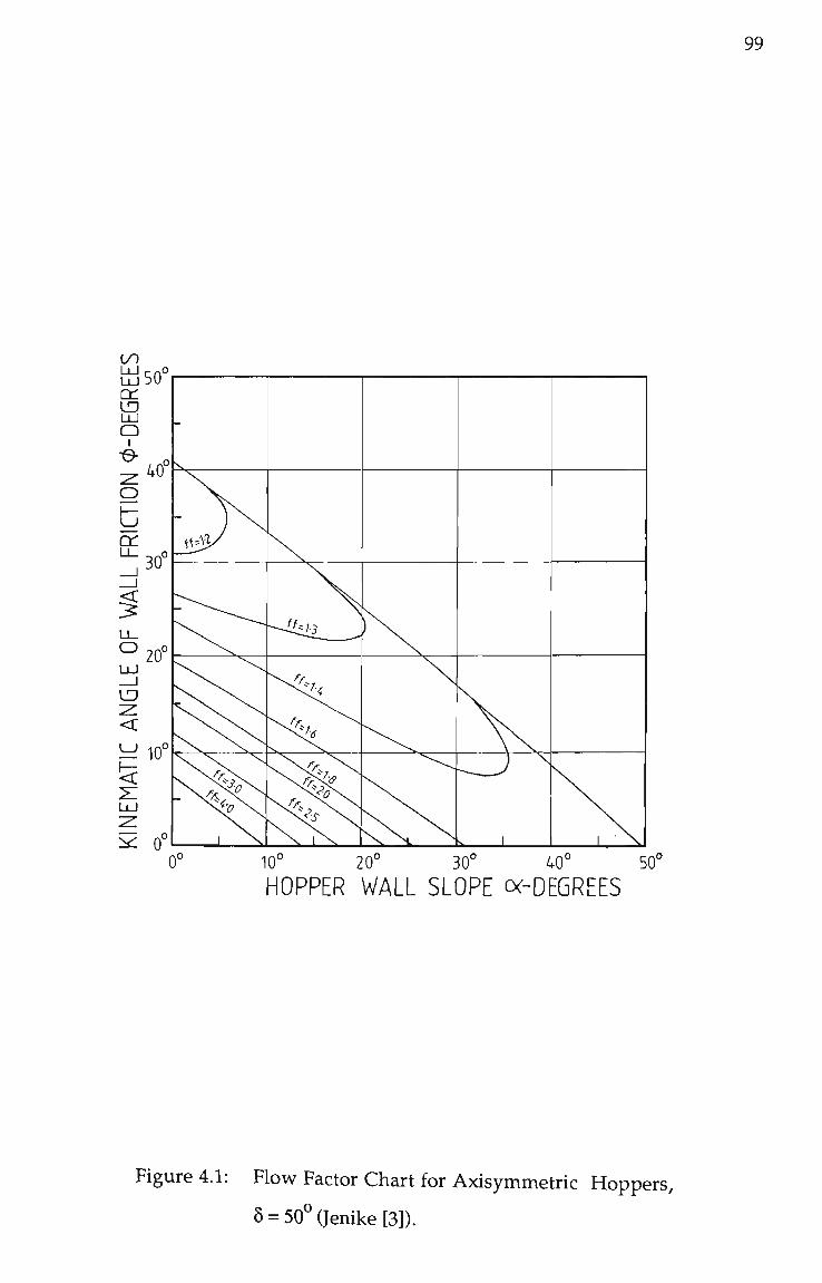
99

50 I/) LU LU Q:

o

30

^ 2 0 ° 11 I

<

\=1 10°

^ 0

•sv

J ^

^

^ s ^ s - r V

^

^^tii__-

\

^ 1 1 \

10' 20' 30' 40' 50° HOPPER WALL SLOPE cx-DEGREES

Figure 4.1: Flow Factor Chart for Axisymmetric Hoppers,

6 = 50° (Jenike [3]).

100

10° 20° 30° 40° 50°

HOPPER WALL SLOPE (X-DEGREES 60°

Figure 4.2: Flow Factor Chart for Plane Flow Hoppers,

8 = 50° (Jenike [3]).

101

flow factor values along the design boundary, they are disadvantaged by the

necessary parameter interpolations required. These are two major problems

associated with the parameter interpolations. Firstly, since the charts are

presented for specific values of 5, those designs having intermediate values

require the parameters of flow factor and hopper wall slope to be adjusted

between the respective charts to ensure accuracy. Secondly, due to the

troughed form of the flow factor contours in the region of the design limit,

determination of the flow factor values can be difficult. For example,

consider determination of the flow factor for ^ of 15 and a of 40 from

Figure 4.2.

A clearer indication of the influence of a on the limit of hopper

wall slope for mass flow in conical hoppers was presented by Johanson and

Colijn [41] (Figure 4.3). This diagram condenses the mass flow limits of the

Jenike flow factor charts to one diagram by displaying contours of constant 5

as a function of (j) and a. Interpolation of intermediate values of 5 in order

to determine the maximum values of a is more convenient than for the

Jenike flow factor charts.

Johanson and Colijn [41] also include an alternative series of flow

factor charts to determine the flow factor after a suitable hopper wall slope

has been selected from Figure 4.3. These charts display contours of constant

flow factor as a function of 5 and (j) for the specific a values of 10, 20, and 30°.

The flow factor chart for a hopper wall slope of 20° is depicted in Figure 4.4.

Interpolation between the flow factor contours is more convenient in this

presentation due to their more uniform nature. However, imprecise flow

factor values can arise because of the presentation of the charts in 10°

increments of wall slope.

Limits on the selection of hopper wall slope have also been

prepared for axisymmetric and plane flow hoppers for mass flow by Arnold

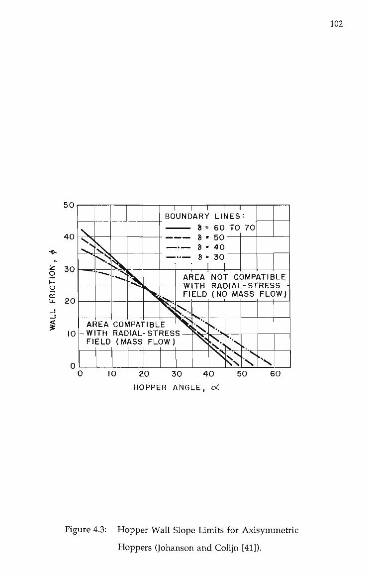
102

I -o CC

g

50

40

30

20

10

BOUNDARY LINES:

8 = 60 TO 70 8 - 5 0 8 « 4 0

0

AREA NOT COMPATIBLE WITH RADIAL-STRESS FIELD (NO MASS FLOW)

AREA GOMPA WITH RADIAL-STRESS FIELD (MASS FLOW)

NTH 0 10 20 30 4 0 50 60

HOPPER ANGLE, oC

Figure 4.3: Hopper Wall Slope Limits for Axisymmetric

Hoppers (Johanson and Colijn [41]).

103

«o

O

a: a. LL.

o UJ

o

LiJ > H O UJ U. I i . UJ

10 20 30 40 50 WALL FRICTION ANGLE, i>

60

Figure 4.4: Critical Flow Factors for Mass Flow Hoppers,

a = 20 (Johanson and Colijn [41).

104

et al. [4] and are presented in Figure 4.5. This presentation utilises the limits

proposed by Jenike [3]. Of more benefit, however, particularly in regard to

computer applications, are the equations which are given to represent the

design limits. For axisymmetric hoppers,

a = 0.5 {l80 - cos - \ ^ ) - [4, + sirC^C^]] (4.3) 2sin5 sinS

and for plane flow hoppers,

exp[3.75(1.01)(^-^°/^»>]-(l) " " 0.725(tan5)0-2 ^ - ^

for ())< 5 - 3; (j) and 5 in degrees.

Reference to Figure 4.5, however, indicates that for the range of

common values of ^ (approximately 15 to 30 ) for mass flow design the

maximum bound of a is relatively insensitive to the variation of 5. The

influence of the effective angle of internal friction on the flow factor has

been considered by Jenike [42]. In dealing with plane flow hopper design he

notes that the effect of ^ is minimal on the flow factor value and presents

the variation of the flow factor as a function of 5 (Figure 4.6). Although

Figure 4.6 was prepared for (|) of 25 and a of 25°, Jenike states that the flow

factor variation will be negligible for different design values, thus having

littie effect on the outlet dimension B from Equation 1.2.

Carson and Johanson [43] have recently enhanced this concept by

adding the flow factor variation with 5 curve for the axisymmetric case.

Figure 4.7. They further comment that the flow factor for both axisymmetric

and plane flow hoppers are essentially the same for the same 8 value (the

value of (j) and a was not stated in the preparation of Figure 4.7).

4.3 ALTERNATIVE PRESENTATION OF THE MASS FLOW

HOPPER DESIGN PARAMETERS

A common factor between the various methods discussed in the

105

tn

LU CC a LLJ a

1— u DC

(X

o LU _l tJ 2 CC

u

CC

LU

PLANE FLOW HOPPERS

RXISTMMETRIC HOPPERS

10 20. 30. 40. HOPPER WRLL SLOPE - DEGREES

Figure 4.5: Wall Slope Limits for Axisymmetiric and Plane

Flow Hoppers (Arnold ef a/. [4]).

106

Od

o y -LJ <

o

Qo 30O 50O 70O 90O

EFFECTIVE ANGLE OF INTERNAL FRICTION


Internal Friction, a = 25°, (|) = 25° (Jenike [42]).


Friction (Carson and Johanson [43]).

107

previous section for the presentation of the flow factor and the hopper wall

slope is the need to refer to several graphs in determining a satisfactory

design.

Generally, the selection of the mass flow hopper geometry

involves the determination of the maximum hopper wall slope allowable

for the particular bulk solid flow properties and operating conditions. This

necessarily involves selecting design values along the mass flow limits

(refer to Figures 4.1 and 4.2) and, as such, the remainder of the bounded

mass flow region is of little interest. These areas are only utilised for such

tasks as the verification of existing plant designs.

With these factors in mind, an alternative presentation of the

mass flow hopper design parameters has been developed and is presented

in Figures 4.8 and 4.9 for axisymmetric and plane flow hoppers respectively.

These figures display the variation of the flow factor and hopper wall slope

in contour form as a function of the kinematic angle of wall friction and the

effective angle of internal friction.

The data mesh for the formation of both charts was obtained by

utilising the design bound for a (as predicted in Equations 4.3 and 4.4) and

the particular values of (() and 8 to determine the maximum allowable value

of a. With these three parameter values the respective flow factor was

determined using differential equation solution techniques and Equation

4.2. Thus, only the values of maximum a which will ensure mass flow for

the respective values of ^ and 8 are displayed.

The following design constraints have been taken into account in

determining the data mesh:

• For Axisymmetric hoppers, a 3° reduction of the hopper wall

slope from the radial stress compatibility bound has been used

108

t s LO

LO ^

ca ^

IT) m

s) CO

m rNJ

cs OJ

IHd - NOIIDIUJ 1lbM dO 310Nd 3I1HW3NIM

Figure 4.8: Alternative Presentation of Axisymmetric Hopper Design Parameters.

109

ca LO

LO '^

cs ' i-

Ln CO

cs en

LO CM

cs OJ

in cs LO cs

IHd - N O U D i y j 11HM JO 310Ny 3I1HW3NIM

Figure 4.9: Alternative Presentation of Plane Flow Hopper Design Parameters.

110

and the flow factor determined at this margin point.

• For plane flow hoppers, the wall slope limit specified in Equation

4.4 and the constraint of (]) > 8 - 3 degrees, has been applied.

• The upper limit of the hopper wall slope is 60°.

This data mesh lends itself to computer applications for systems

that do not have mathematical packages for the solution of differential

equations (to determine the flow factor). The values required can be

determined by linear interpolation techniques based on the data mesh.

An advantage of this chart format is that a complete overview of

the trends of flow factor and hopper wall slope variation with ^ and 8 is

presented. Reference to Figures 4.8 and 4.9 indicates the direct influence of ^

on the value of a and the minor effect of 8, particularly for plane flow

hoppers. This trend of reducing values of flow factor with the increasing 8 is

also well demonstrated. This trend is in agreement with the presentation of

Jenike [42], but allows the overall effect of ^ on the flow factor to be

appreciated. For a constant 8 value of 50 and a range of (|): 5° < (j) < 40°, the

flow factor is seen to vary from 1.25 to 1.22, justifying the assumption of

Jenike to neglect the ()> variation in determining an initial measure of

flowability.

For a given set of values for 8 and (]), the design parameters of a

and flow factor are determined by referencing the intersection point to the

plotted contours. Although the contour increments for Figures 4.8 and 4.9

are necessarily coarse to ensure clarity, large chart formats can utilise

smaller contour intervals and reduce prorating of values.

Correct interpretation of the data determined from the charts

should be stressed. It is important to bear in mind that only the maximum

value of a and the respective flow factor value relevant to the traditional

I l l

mass flow limits are displayed. Concerning the value of hopper wall slope,

the a contour specified the maximum value allowable to ensure mass flow

and slip of the bulk solid along the wall. Values of a greater than that

specifies can lead to a funnel flow discharge pattern, while a reduction

below this value leads to a more conservative design. Reference to Equation

1.2 similarly provides an insight into the variation of the flow factor about

the design value. Utilising a flow factor value smaller than the design point

will lead to a reduction in a^, a reduced outlet dimension B and, hence, the

formation of cohesive arches. Noting that the design point specifies the

critical flow factor value, a more conservative design will then result from

using an increased value.

The advantages of utilising this presentation to determine the

hopper geometry based on the bulk solid flow properties have been noted in

the preceding discussions. However, care should be exercised in the

verification of mass flow occurring in existing storage facilities. The value

of hopper wall slope can be checked knowing 8 and (j) and ensuring that

^actual " ^charf Difficulties arise in checking the hopper outlet dimensions

(as affected by the flow factor) because values of a not lying on the mass

flow limit in the case of plane flow, or, 3° less than the limit for

axisymmetric hoppers, relate to flow factors not displayed in Figures 4.8 or

4.9. Reference to the original Jenike flow factor charts (Figures 4.1 and 4.2)

indicate that the flow factor may be above or below that displayed in the

alternative presentation, depending on the value of a used within the

bounded mass flow region. It is recommended that for this exercise the

Jenike charts be consulted because the complete flow factor variation with a

is displayed for given values of ^ and 8.

4.4 ILLUSTRATIVE EXAMPLE

To demonstrate the use of these new design charts, the geometry

112

of a mass flow hopper with a plane flow outlet for an ROM coal storage will

be determined. The measured flow properties of the coal are presented as a

function of the major consolidation stress a^ in Figure 4.10 and in equation

form in Table 4.1.

Two characteristics, typical of moist cohesive bulk solids such as

coal, are depicted in Figure 4.10. These are the reductions of 8 and ^ (for

some wall materials) to limiting values with increasing o^. The variation of

the wall friction angle may be due to either convex upward wall yield locus

and/or the tendency of the bulk solid to adhere to the wall lining material

at low values of normal stress.

A portion of Figure 4.9 is presented in Figure 4.11, which displays

a contours at 1 increments and the flow factor contours at 0.01 intervals.

As previously stated, an iterative procedure must be used to determine the

critical hopper geometry if either 8 or (j) vary with o^. Essentially, the

procedure suggested by Jenike [3] will be applied, first determining the

critical flow factor value, noting the respective a value and then applying

the flow factor value to Equation 1.2 to yield the hopper outlet dimension.

The procedure is deemed to have converged to the critical values when

little change results in a^ and 8 from successive iterations.

Consider the determination of the hopper geometry under

instantaneous conditions with the UHMW polymer as the wall lining

material. To start the procedure initially estimate 8 = 60 . With (j) = 23 and

constant, from Figure 4.11 point A yields a flow factor value of 1.111.

Applying the flow-no flow concept to the instantaneous flow

function and the respective flow factors produces an initial value for o^ of

2.07 kPa.

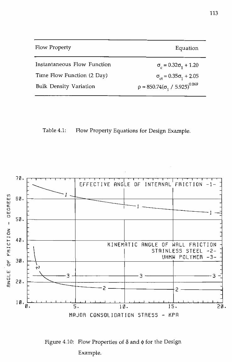
113

Flow Property Equation

Instantaneous Flow Function

Time Flow Function (2 Day)

Bulk Density Variation

o = 0.32O, + 1.20 c 1

a , = 0.350^ + 2.05 ct 1

0.069 p = 850.74(a^ / 5.925)

Table 4.1: Flow Property Equations for Design Example.

70.

tn LU lU CC u UJ n 1

z o 1—I 1 -u t - t

OC u. ll . o iLl _J {•) 2 (X

60.

b0.

40.

30.

20.

10.

- I — T — 1 — r - i — 1 — I — r

. ^3

A.

I • I • I . I

0.

1 — ' — I — ' — r - J — ' I • r T — • — I — > — I — ' — I — ' -

EFFECTIVE RNGLE OF INTERNRL FRICTION -1- I

KINEMRTIC RNGLE OF WRLL FRICTION STRINLESS STEEL -2-

UHMW POLYMER -3-

J I 1 I 1-

3 -:

J I I 1 L

5. 10. 15. 20.

MRJOR CONSOLIDRTIGN STRESS - KPR

Figure 4.10: Flow Properties of 8 and ^ for the Design

Example.

114

9330030 - NOIiOiyj 11HM 30 310NH 3I1HW3NIM

Figure 4.11: Determination of the Hopper Geometry for the

Design Example.

115

That is for the following equations:

flow function:

flow factor:

and at the critical design

and

a = 0.32O, + 1.20 c 1

ff = ^ = ^1

point, o^ =

^ c = ^ r

1.111

o . Then c

"1.111

1 r^Ort J. 1

Solving for Cy

and hence

aj(Y-^-0.32) = 1.20

o^ = 2.07 kPa.

Reference to the 8 variation depicted in Figure 4.10 for this value

of a yields an updated value of 8 of 64.5 .

The subsequent values for each iteration in converging to the

critical values are presented in Table 4.2. For the values of 8 (64.6 ) and ^

(23.1 ), the flow factor and a can be read from Figure 4.10 as 1.079 and 30.3

(say 30.5 ) respectively. As indicated in the above table, convergence occurs

relatively fast. Substitution of the relevant values into Equation 1.2 allows

the critical outlet dimension to be determined. From the graphical

presentation of H(a) [3] (or alternatively Equation 5.2),

H(a) = H(a = 30.5) = 1.15

and

p = p (CT = 1.98) = 788.1 kg/m^

and hence B = 273mm (say 275mm). The critical hopper geome t ry

parameters would then be detailed as a = 30.5 and B = 275mm.

The procedure becomes further complicated when considering a

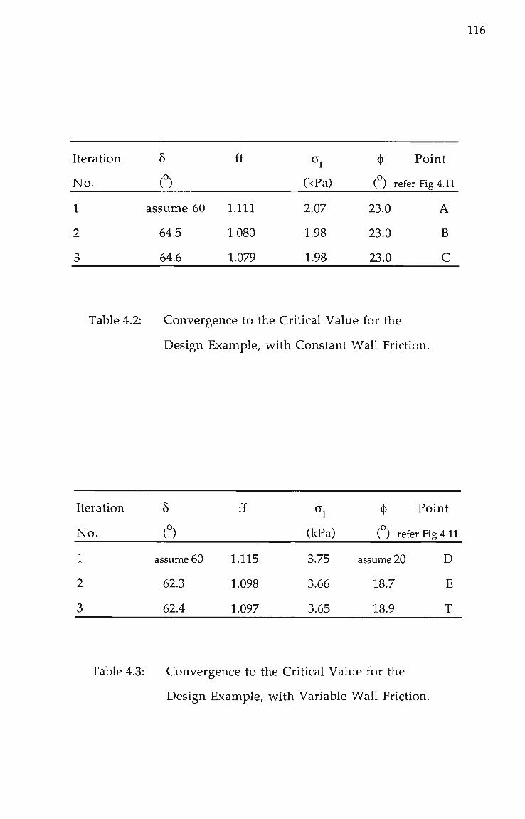
116

Iteration

No .

1

2

3

8

(°)

assume 60

64.5

64.6

ff

1.111

1.080

1.079

^1

(kPa)

2.07

1.98

1.98

(j) Point

( ) refer Fig 4.11

23.0 A

23.0 B

23.0 C

Table 4.2: Convergence to the Critical Value for the

Design Example, with Constant Wall Friction.

Iteration

No.

1

2

3

8

C)

assume 60

62.3

62.4

ff

1.115

1.098

1.097

^1

(kPa)

3.75

3.66

3.65

({) Point

( ) refer Fig 4.11

assume 20 D

18.7 E

18.9 T

Table 4.3: Convergence to the Critical Value for the

Design Example, with Variable Wall Friction.

117

lining material that has a variable kinematic angle of wall friction. To

illustrate the design procedure when both (j) and 8 vary with Oy the critical

geometry parameters will be determined for time storage conditions (2 days

at rest), using stainless steel as the wall lining material. In a similar fashion

to the previous example, values of 8 and (j) must be assumed to obtain an

initial flow factor value. Assuming 8 = 60 and ([) = 20 , the iteration values

are presented in Table 4.3

For the final values of flow factor ff = 1.097 and a = 35.5°, the

critical outlet dimension can be determined as 485 mm, with H(a) = 1.18

and p = 822.5 kg/m^.

The variation of (j) with o^ can be utilised in mass flow hopper

design by allowing larger wall slopes for outlet dimensions greater than the

critical value determined in relation to particular instantaneous or time

flow functions. The hopper wall slope may be increased due to the

reduction on wall friction which occurs from the increased values of o^

resulting from increased outlet dimensions. The variation of a with B can

be determined by incrementing o^ above the critical value, calculating the

respective values of <t> ^rid 8 and, from Figure 4.11, reading the respective

values of a and the flow factor. Knowing the flow factor and the value of a

allows the outlet dimensions to be calculated.

The variation of 8 and (j) for a range of o^ has been presented as a

curve in Figure 4.11. This curve is unique to the particular variations of (j)

and 8 with o^ and, as indicated, the critical design points for instantaneous

(point I) and time storage (point T) conditions lie on this locus.

118

Oj (kPa)

1.98

2.50

3.00

4.00

5.00

8.50

10.00

15.00

8(°)

64.6

63.9

63.2

62.0

61.0

5.81

57.1

54.7

<^C)

21.7

20.4

19.6

18.6

18.0

17.0

16.8

16.4

ff

1.080

1.086

1.091

1.100

1.109

1.134

1.143

1.168

a( )

31.8

33.4

34.5

35.8

36.6

38.0

38.3

39.0

B(mm)

275

342

405

528

647

1042

1204

1724

Table 4.4: Variariation of Outiet Dimension and Hopper

Wall Slope with Increasing Major

Consolidation Stress for the Design Example.

119

Table 4.4 summarises the variation of ^ and 8 with o- and the

resulting variation of a with B for stainless steel. It can be seen that for

plane flow hopper outlets in the region of 1 metre width, wall slopes of 38

could be utilised. This design data can also be applied to increasing the

hopper wall slope in a stepwise fashionat intermediate levels above the

hopper outlet. As the effective width of the hopper increases due to

divergence of the walls, the wall slope can be increased in accordsmce with

the above variation. This technique can prove useful in design applications

that have headroom and space constraints and also in determining the

extent of hopper wall linings.


The advantages resulting from this presentation over existing

methods include:

• The ability to obtain an overall assessment of the variation of the

design parameters of a and flow factor along the limits of mass

flow chosen for design purposes.

• All the relevant design data required for hopper geometry

determination are presented on one chart (for either

axisymmetric or plane flow hoppers), which reduces the amount

of parameter interpolation required.

• A characteristic curve can be plotted on the chart presentation

representing the variation of ^ and 8 with increasing Cj The

critical values of (|) and 8 for instantaneous and time storage

conditions lie on this curve. The respective values of a and flow

factor as specified by the curve can be utilised to present the

variation of a for values of B greater than the critical.

• The data mesh used to determine the contour positions on the

chart can be applied to compile a hopper design computer

120

program using linear interpolation techniques (rather than the

solution of differential equations) to determine the required

design parameters.

These hopper design parameter charts have recently been

incorporated into the new Draft Code Practice for the Design of Silos and

Bins prepared by the British Materials Handling Board. [44].

121

CHAPTER 5

GRAPHICAL DETERIVUNATION OF THE ]VIASS FLOW

HOPPER GEOMETRY PARAIVIETERS

5.1 INTRODUCTION

The determination of the geometry of mass flow hoppers is based

on the design data of the critical hopper outlet dimension B and the

maximum values of wall slope a, for both instantaneous and time storage

conditions, and graphs of the variation of hopper wall slope with outlet

dimension for each wall material considered. This method of design data

presentation, particularly regarding the a versus B charts has a number of

disadvantages.

Firstly, to produce the a versus B graphs without the aid of

computers can be a complicated and tedious task, requiring reference to the

relevant flow properties and hopper flow factor charts. To employ computer

techniques, on the other hand, requires a powerful computer and the

necessary algorithms and mathematical support code to generate flow

factors from first principles. As presented by Arnold et al. [45] and Moore et

al. [46] the development of such programs is an involved and complex task.

(Chapter 7 discusses the development of computer software for flow

property processing and bin design).

A second aspect of the current hopper geometry data presentation

methods is the failure to relate the critical hopper geometry to the

experimental flow properties, or to the design stress values acting at the

hopper outlet. It would be helpful, particularly in the design for difficult

cohesive bulk materials, to allow an insight into the design procedure and

an appreciation of the sensitivity of results due to flow property variations.

122

A further consideration is the difficulty in relating hopper design

parameters with experimentally determined flow properties when applying

computer techniques to process the flow property data and determine the

critical hopper geometry parameters. The use of computers can cause the

design engineer to lose sight of the basic flow property data in its application

to hopper design. In the computer procedures, flow properties such as the

flow function, are represented by curve fitting an assumed empirical

function form to several discrete data points. This can lead to significant

errors if the fitted curve is not an accurate representation of the complete

flow property. Using the current presentation of design data the following

useful trends and relations cannot be easily visualised:-

• the sensitivity of changes in the flow function position on the

minimum opening dimension. This is important for low values

of a^ removed from the experimental data points,

• the correlation of the hopper wall slope with the angle of wall

friction,

• the relation between hopper outlet dimension and Gy

To eliminate some of the present difficulties^ an alternative

graphical method of design data presentation in the form of design

nomograms has been developed which clearly shows the relation between

the hopper geometry parameters and the experimentally determined flow

properties. The graphical design nomograms represent a compact,rapid

method of manually determining the mass flow hopper geometry

parameters.

This chapter details the determination of mass flow hopper

geometry parameters using the graphical design nomograms, which were

developed by combining the concepts and graphical formats introduced

from the alternative presentation of the hopper design parameters (Chapter

123

4) [47] and the novel method of presenting mass flow hopper geometry

parameters developed by Moore and Arnold [48].

5.2 NOMOGRAMS FOR MASS FLOW HOPPER DESIGN

Design nomograms or graphical worksheets have been developed

for axisymmetric and plane flow hopper design, and are presented in

Figures 5.1 and 5.2 respectively. Figures 5.3 and 5.4 present alignment

nomograms for the calculation of the critical outlet dimension B for

axisymmetric and plane flow hoppers respectively.

Referring to Figures 5.1 and 5.2, the layout of the nomograms

essentially allows the presentation of the bulk solid flow properties (as a

function of o^) on the left side and the alternative hopper design parameter

chart (ff and a) on the right. To use the nomogram, the bulk solid flow

properties are first drawn against the respective axes. Note the ^ versus a,

variation determination depends on the wall yield locus and the effective

angle of friction, and, involves Mohr circle stress analysis as reported in [45]

(refer to Appendix I). A separate nomogram or worksheet is prepared for

each hopper wall material that is considered.

The first step in operating the nomogram is generating the 'flow

factor locus'. An arbitrary o^ value is selected and by projecting this value

vertically the corresponding values of ^ and 8 are found. These two friction

values are then projected onto the hopper design parameter chart and the

corresponding values of ff and a read from the intersection point. In the

lower left work space, using the flow factor scale, the intersection between

the ff and a^ values is plotted. This is one point on the flow factor locus.

The flow factor locus is the curve passing through the coordinates ^1

i^yTf) displaying the variation of the flow factor with respective values of

Gy

124

3 UJ

M

be

HAJOR CDNSCH.I0AT1ON STRESS, a", kPa

HOPPER GEOMETRY FOR MASS FLOW (AXISYMMETRIC)

Figure 5.1: Design Nomogram for Axisymmetric Mass

Flow Hoppers.

125

MAJOR CONSOLIDATION STRESS, o'j KPq

Figure 5.2: Design Nomogram for Plane Flow Mass Flow

Hoppers.

126

MAJOR STRESS IN ARCH,o' KPa

pO.S

BULK DENSITY

600 r

700

aoo

900

1000

CRITICAL ARCHING DIMENSION.B •• rise

-200

2S00

Figure 5.3: Alignment Nomogram for Calculation of

Outlet Dimension, Axisymmetric Hoppers.

127

BULK DENSITY •9 Ko/m-5

CRITICAL ARCHING DIMENSION,B nn

200 MAJOR

STRESS IN ARCHdikPa rO.4

l<J.5 F300

600r

700

BOQh

900

1000

' SSOO

Figure 5.4: Alignment Nomogram for Calculation of

Outlet Dimension, Plane Flow Hoppers.

128

This curve is unique to the particular bulk solid, being dependent

only on the angle of wall friction, the effective angle of friction and the

shape of the hopper outlet (axisymmetric or plane flow).

The flow factor locus does not usually pass through the origin, but

begins at the first value of a^ that yields (|) and 8 for which a flow factor for

mass flow can be determined. For wall materials displaying high levels of

adhesion with the bulk solid this first value of a^ can be as high as 2.5 - 3.0

kPa.Note that if <^ and 8 for the bulk solid are constant, then the flow factor

locus will be a straight line indicating a constant ff (and 8) for all values of

Cy

The value of a (determined at the same time as ff) can be plotted

against the o^ abscissa corresponding to the hopper wall slope scale

provided.

The value of the hopper outlet dimension B is determined from

the alignment nomograms (Figures 5.3 and 5.4) which solve Equation 1.2,

and include functional scales for H(a) (presented graphically in [3]). These

nomograms could be deemed unnecessary with the common application of

electronic calculators, particularly if the relations presented by Arnold et al.

[4] for H(a) are utilised.

For axisymmetric hoppers: , , (130 +a ) , ,

H(a) = (5.1) 65

emd for plane flow hoppers:

where a is in degrees.

Referring to these figures, first, line (i) is drawn between the p scale (for the

relevant p value corresponding to a^) and the a value. This provides an

129

intersection point on the reference line from which Une (ii) is projected

through the o^ value and onto the critical arching dimension scale. The o^

value is determined by projecting the flow factor - o^ intersection point onto

the a J axis (in the lower left work space) or by solving CTJ = -rr . The

subsequent value of B can then be plotted along the o^ abscissa

corresponding to the critical arching dimension axis provided.

The above operations are repeated for a range of o^ values ranging

from perhaps 1 kPa to 15 kPa to allow curves to be plotted providing the

following parameter variations as a function of major consolidation stress,

Gy

• the flow factor locus,

• the hopper wall slope, a,

• the hopper outlet dimension, B.

The hopper geometry parameters for instantaneous and time

storage consolidation conditions are determined by establishing the critical

a^ value, where the appropriate flow function intersects with the flow factor

locus. The critical values of a and B can then be read from the respective

plotted curves for the appropriate o^ value.

5.3 ILLUSTRATIVE EXAMPLE

A design example using the nomogram to determine the hopper

geometry parameters for a plane flow slot outlet hopper storing black coal is

provided in Figure 5.5. For convenience. Figure 5.6 provides an enlarged

presentation of the lower left portion of Figure 5.5. The required flow

properties have been plotted in the appropriate section on the left side of

the graph.

130

-^... 4

MAJOR CONSOLIDATION STRESS, o'j kPa

HOPPER GEOMETRY FOR MASS FLOW

(PLANE FLOW)

Figure 5.5: Determination of the Plane Flow Hopper

Geometry for the Design Example.

131

(, 0

(/) (/) III a. W

El-D

H >.

PI

z H

i

a a JC 1

ro" _•«

6 <

z

{/i (/) u ^ V)

CC

0* > I I M-

p-^Lua. •H I I I I I I I I I I I I I I I I ' I

I I 1 . 1 1 I I • I . 1

1 5 0 0

I I I I 1 I

35*

000

500

6 8

OQ

2 O H w z UJ

z H X u OC <

- I < u H H-M a u

MAJOR CONSOLIDATION STRESS^ o'j hPa

Figure 5.6: Determination of the Plane Flow Hopper

Geometry for the Design Example (enlarged

portion).

132

Selecting a value of o^ = 5kPa to illustrate the procedure,

projecting this value (line (a)) to the 8 and <]) flow properties, values of 61°

and 18 respectively are found. These values are projected (lines (b) and (c)

onto the hopper design parameter chart and intersect at point 1, yielding

values of ff = 1.11 and a = 37°. Drawing in the flow factor ray of ff = 1.11

determines intersection point 2 with Oj = 5 kPa. Point 3 for a = 37° can also

be plotted against the appropriate scale. Using the alignment nomogram, B

is determined for the values : p = 840 kg/m^, o^=—= TTT= 4.5 and a = 37°.

The value of B = 650 mm is found and plotted at point 4. This procedure has

been repeated to generate the complete flow factor locus and the a and B

variations.

The critical hopper geometry parameters for instantaneous and

time consolidation conditions are determined from the intersection of the

relevant flow function with the flow factor locus. For the critical a^ value

found, the corresponding values of a and B are noted.

Then, for instantaneous conditions:

Point 5, a = 32.5°, B = 350 mm

and for time storage conditions:

Point 6, a = 35.5°, B = 540 mm.

Often, the exact position of the flow function may not be known

accurately because it generally results from drawing a line through three

experimentally derived points from the instantaneous or time yield locus.

The sensitivity of the a and B values to variations in the location of the

flow function can be assessed easily .

For example, in Figure 5.6, it can be seen that changing the flow

function to FFT2 yields a new intersection, point 7, between the flow

function and the flow factor locus. This intersection point defines a value of

133

a J = 5 . 8 kPa with consequent a and B values of 37.5 and 740 mm

respectively.

This section of the worksheet indicates that flow functions may

have different characteristics and yet still lead to similar critical hopper

geometry parameters, for example, a flow function with high initial

cohesion with a small gradient compared to a flow function with a low

cohesion but steeply sloping.

Perhaps a more important feature that is highlighted by this

presentation is the degree of influence (j) has on the hopper geometry. For

many bulk solids, the outlet dimension of hoppers will exceed the critical

value, (ie. Point 5, for instantaneous conditions). Thus the subsequent

geometry need only follow the prediction of the a versus o^ and B versus a^

curves, which are predominantly under the influence of the (}> variation.

This feature provides an effective method for the experienced

designer to determine the hopper geometry parameters based on a reduced

flow property testing program. Only the wall friction and compressibility

tests are required, tests which are rapid and relatively straightforward

compared to shear testing (note that the important wall friction parameter

can be determined on any suitable Coulomb friction tester).

Based on experience, the effective angle of internal friction, 8,

possible flow function positions and B can be estimated. The discussions of

Chapter 4 have highlighted the limited sensitivity of ff and particularly a to

variations in 8. Thus the a versus a^ and B versus Oj design curves can be

generated and extremely useful hopper design information achieved.

The detailing of the hopper geometry as part of a bulk solids

handling system often requires attention to such constraints as allowable

head room, maximum lump size, feeder arrangements, proposed discharge

134

flow rates and economy of design for the required storage tonnage. The

hopper wall slope and outlet dimension design curves allows the design

engineer to confidently vary each parameter above the critical value to

satisfy any constraints acting. For example, if the slot outlet width has to be

constrained to some value above the critical, the hopper wall slope could be

increased according to the design curves allowing a reduced hopper height

and relief to possible headroom problems.

A further application of this presentation is the ability to optimise

the selection of a and B in regard to feeder loading. For example, utilising

Reisner's theory [4] for the calculation of the flow load, the major

consolidation pressure a^ at the hopper outiet is assumed to act vertically on

the feeder. The value of Oj can be found by rearranging Equation 1.2:

yBff

and hence the total flow load, Q, can be determined from

Equation 5.4:

Q = ajA (5.4)

where A is the cross-sectional area of the hopper outlet. It would be

straightforward to provide a additional graph of Q versus o^ (in a similar

format to the other flow properties or design parameters), allowing a direct

indication of the feeder flow loading with increase of the outlet dimension.

Alternatively, Q could be conveniently calculated at point values of B as the

current worksheet format dearly depicts the required B and G^ values.


The design nomograms presented in this chapter provide a

compact and accurate method for the manual calculation of the mass flow

hopper geometry parameters. The presentation has advantages over

135

existing methods in that the relation between the flow properties and the

hopper geometry is clearly illustrated, the hopper design parameter chart

requires no interpolations and the sensitivity of geometry parameters may

be examined in view of doubtful or dubious flow property variations

The procedure described here also lends itself to computerisation,

with computer graphics being used to produce the final design graphs.

These aspects will be further developed in Chapter 7.

136

CHAPTER 6

STANDARDISED HOPPER

GEOMETRY DESIGN GUIDELINES

6.1 INTRODUCTION

Review of the critical hopper geometry parameters presented in

Table 3.1 and of the flow property values in Table 2.1, raises the feasibility of

utilising standard design guidelines for the determination of the hopper

geometry parameters of a and B for mass flow. This is achieved by

determining the expected ranges of a and B, dependent on the moisture

content of the coal and secondly by analysing statistically determined flow

properties allowing a reduced flow property testing procedure to be

formulated.

Advantages of such a procedure include:

• Reduction of the amount of flow property testing required for the

design of coal storage bins. For storage facilities that handle

several different coals (eg. an export market coal loader) a

relatively large amount of time and expense is required for flow

property testing to identify the worst case bulk solid, to define the

design criterion.

• Often coal storage and processing facilities are detailed without an

appreciation of the principles of bulk storage and flow [18].

Utilisation of such guidelines would increase the awareness of

industry and encourage a systematic approach to the design of

coal storage fadlities.

• Allow the accurate preparation of initial arrangement layouts of

coal storage facilities early in the design process. This would be

particularly useful for facilities for which no bulk samples exist.

137

such as new mine developments where only bore hole samples

are available. This approach would highlight storage geometry

constraints earlier, and also allow more accurate costing estimates

to be prepared.

Several authors have conducted studies in this direction, ter Borg

[31, 49] and Dau [32] have investigated the flow properties and subsequent

mass flow hopper geometry parameters for large numbers of bulk solids for

statistical application in the chemical industry. Figure 6.1 presents, for a

survey of 500 bulk solids [31], the percentage of bins that would successfully

operate in mass flow as a function of the hopper wall slope angle. As

indicated, for axisymmetric hoppers with a^ = 30 , only 25% of installations

would be expected to mass flow. However, silo designers and manufacturers

of packaged and purpose - designed silos still regard this slope as

sufficiently steep. Referring to the plane flow variation (which is increased

from the axisymmetric case by 8°- 10°, Schwedes [50]), for a = 30°, 50% of

installations would be expected to operate in mass flow.

The second aspect of hopper design, the determination of the

outlet dimension, has been investigated statistically by Sinkwitz [51] and

Horn [52]. Sinkwitz attempted to apply a cohesive arch or bridge-forming

probability to yield hopper outlet dimensions (with a success risk factor)

smaller than the outlet dimensions determined by the Jenike method [3].

This approach aimed to reduce the amount of overdesign which has been

indicated by several experimental studies, and recently discussed by Jenike

[53].

6.2 TERMS OF REFERENCE

In developing this concept, the interaction of the coal (represented

by the respective flow properties) and the operational characteristics of mass

flow bins must be taken into account. The heterogeneous nature of black

138

\-) ID Q

100

— •

§^80 n Ll_

o CC

3 0 ...1

^ 6 0 UJ CO CD (y)

s: < ^ ^ A O U J

>

<r _ j

ZD 7-Z3

z I D ^ ^ ^ p20 < CC L U

% 0

'AXISYMMETRIC

PLANE FLOW

10 20 30 ^0° HOPPER WALL SLOPE, «c ^ P

Figure 6.1 Bulk Solids with Mass Flow as a Function of

Hopper Wall Slope (ter Borg [31] and

Schwedes[50]).

139

coal (physically and chemically) is well known, leading to variations in the

flow properties of different coals and their relative flowability. Colijn and

Vitunac [54] note that there appears to be no such product as a 'typical coal'

or an 'average coal' in a similar manner to there being no 'typical soil' for

soil mechanics to work with. For these reasons, the coal types applicable for

this procedure are restricted to similar coals used in the test work. These

coals could be defined as:

Hard Black Coals.

Bituminous to Semi-Anthracite Rank,

Hardgrove Grindability Index : HGI < 60.

Ash Content (non swelling clay) < 15%.

Similar particle distributions as defined by the Rosin-Rammler

Distribution Parameters.

The ash content has been specified in broad terms only. For those

clay types that are known to lead to handling problems flow property testing

will have to be undertaken and the traditional design approach employed.

The Hardgrove Grindability has been specified to restrict coals to the harder

and less friable coal types. The testwork has highlighted the increased

storage problems due to the increased cohesive strength that occurs for

friable coals, due to the increased fines content caused by degradation from

repeated handling operations. Most coals tested in the program displayed

similar particle distributions for the as received samples resulting from

isotropic breakage and obeying the Rosin-Rammler Distribution. The

Rosin-Rammler Distribution Parameters presented in Table 6.1 for the coals

tested demonstrates this feature.

The moisture content of the coal was shown to be a significant

parameter. For the coals from the Southern Coalfield the maximum outiet

spans occurred for the moisture range of 10% - 15%. Coal samples below

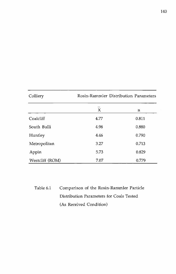
140

Colliery Rosin-Rammler Distribution Parameters

X n

Coaldiff

South Bulli

Huntley

Metropolitan

Appin

Westdiff (ROM)

4.77

4.98

4.46

3.27

5.73

7.07

0.811

0.880

0.790

0.713

0.829

0.779

Table 6.1 Comparison of the Rosin-Rammler Particle

Distribution Parameters for Coals Tested

(As Received Condition)

141

these levels will be less cohesive and thus more free flowing, while coals

above the 15% level (and possessing the approximate particle distribution

found in the testing program) would be close to the saturated moisture

content. Moisture contents higher than 15% could also indicate high fines

contents or expansive clays present within the ash content.

The design procedure in determining the hopper geometry

parameters aims to achieve a reasonable compromise between such

technical aspects as headroom and capacity requirements, allowable values

of hopper wall slope for various wall lining materials, outlet dimension,

type and size of feeder and feeder loads. There are three basic shapes of mass

flow hoppers, namely, axisymmetric, plane flow and transition (a

combination of a plane flow hopper with conical end walls), as depicted in

Figure 1.2.

Considering the design and operational merits of the various

mass flow hoppers, the following aspects are significant:

• Axisymmetric hoppers operate with a distinct mass / funnel flow

boundary (linking a with (^ and 8) as depicted in Figure 1.3. Plane

flow hoppers, in contrast, have a less distinct operational

boundary between mass flow and funnel flow. To this effect

Jenike [3] states that the plane flow hopper slope may be increased

up to 5 above the design recommendation if the cylinder/hopper

transition is generously radiused rather than meeting at a distinct

intersection,

• As previously stated, the plane flow hopper slope a is generally

9 - 11 greater than the slope required for axisymmetric hoppers.

Thus plane flow hoppers can offer a more economical design in

terms of height [55].

142

• A limitation of plane flow hoppers is the requirement for long

slot outlets (L > 3B). This restricts, to some degree, the type of

feeder used. More particularly, care must be taken to ensure the

outlet is completely live, with the bulk solid being withdrawn

over the complete outlet area. If this does not occur then funnel

flow will develop within the stagnant contents of the bin.

• Pyramidal hoppers are limited because of the in flowing valleys

between each hopper face. These valleys present high friction

regions to bulk solid flow and lead to material hang ups.

Designers will find specifying the hopper valley angle equal to a^

[3] will often lead to impractical hopper proportions. For this

reason it is recommended that only axisymmetric hoppers of

conical form be considered.

The testwork considered three wall lining materials, rusty mild

steel, 304-2B stainless steel and Pactene. For the development of these

guidelines only stainless steel will be considered since its use is well proven

in the coal industry, it offers low wall friction angles, a stable surface finish

after long periods of contact with moist coal and is a reasonably wear

resistant material. Rusty mild steel was discounted due to its high <^ values

and the inherent surface deterioration that occurs from contact with wet

coal by rusting. The Pactene has <^ values intermediate to stainless steel and

rusty mild steel, but may not have the wear resistance required, particularly

for ROM coal storage bins. The flammability and electrostatic properties of

the Pactene also make it unacceptable for underground applications where

spontaneous combustion or dust/gas explosions are possible.

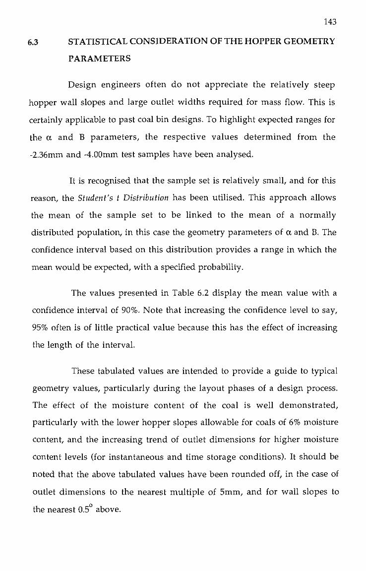
143

6.3 STATISTICAL CONSIDERATION OF THE HOPPER GEOMETRY

PARAMETERS

Design engineers often do not appreciate the relatively steep

hopper wall slopes and large outlet widths required for mass flow. This is

certainly applicable to past coal bin designs. To highlight expected ranges for

the a and B parameters, the respective values determined from the

-2.36mm and -4.00mm test samples have been analysed.

It is recognised that the sample set is relatively small, and for this

reason, the Student's t Distribution has been utilised. This approach allows

the mean of the sample set to be linked to the mean of a normally

distributed population, in this case the geometry parameters of a and B. The

confidence interval based on this distribution provides a range in which the

mean would be expected, with a specified probability.

The values presented in Table 6.2 display the mean value with a

confidence interval of 90%. Note that increasing the confidence level to say,

95% often is of little practical value because this has the effect of increasing

the length of the interval.

These tabulated values are intended to provide a guide to typical

geometry values, particularly during the layout phases of a design process.

The effect of the moisture content of the coal is well demonstrated,

particularly with the lower hopper slopes allowable for coals of 6% moisture

content, and the increasing trend of outlet dimensions for higher moisture

content levels (for instantaneous and time storage conditions). It should be

noted that the above tabulated values have been rounded off, in the case of

outiet dimensions to the nearest multiple of 5mm, and for wall slopes to

the nearest 0.5° above.

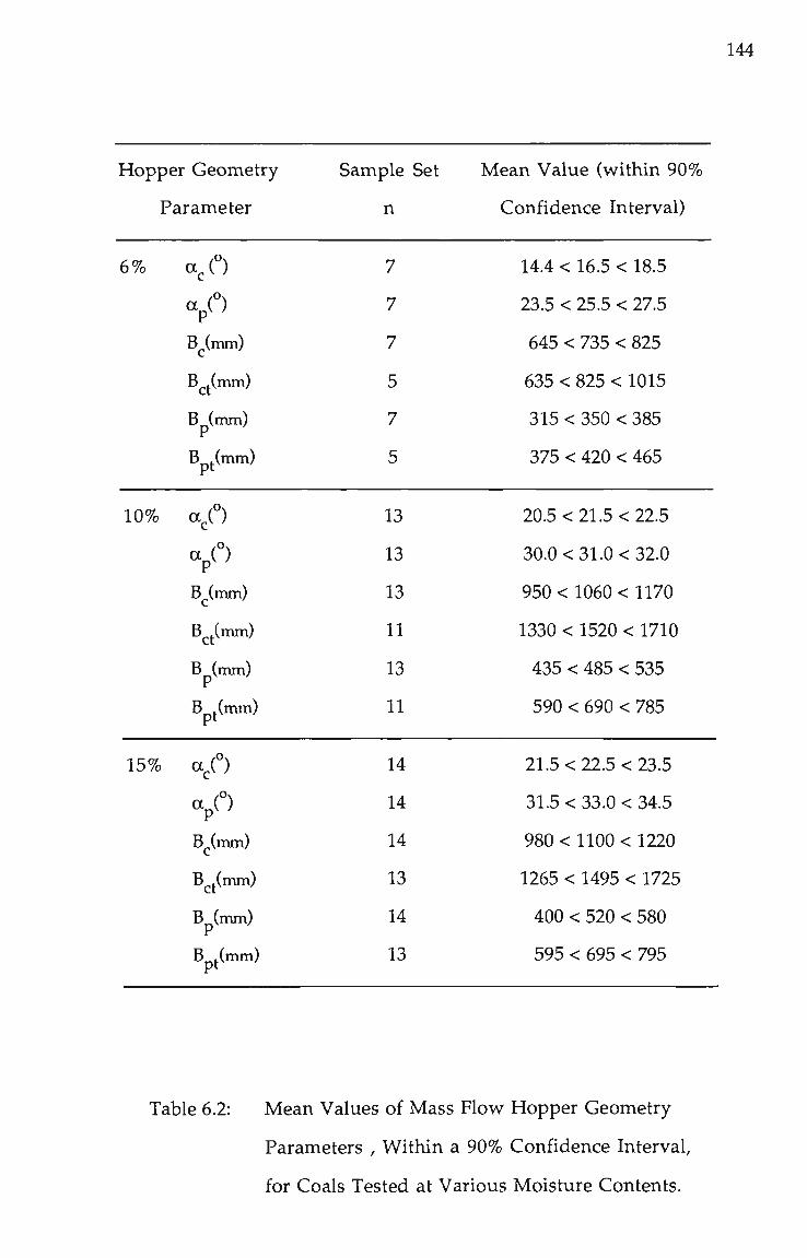
144

Hopper Geometry

Parameter

6%

10%

15%

a^C)

v°> B^(mm)

B (nun)

Bp(mm)

B .(mm)

a/)

a/)

B^(mm)

B^j(mm)

Bp(mm)

B j(mm)

a/)

a/)

B^(mm)

B^j(mm)

Bp(mm)

B j(mm)

Sample Set

n

7

7

7

5

7

5

13

13

13

11

13

11

14

14

14

13

14

13

Mean Value (within 90%

Confidence Interval)

14.4 < 16.5 < 18.5

23.5 < 25.5 < 27.5

645 < 735 < 825

635 < 825 < 1015

315 < 350 < 385

375 < 420 < 465

20.5 < 21.5 < 22.5

30.0 < 31.0 < 32.0

950 < 1060 < 1170

1330 < 1520 <1710

435 < 485 < 535

590 < 690 < 785

21.5 < 22,5 < 23.5

31.5 < 33,0 < 34.5

980 < 1100 <1220

1265 < 1495 < 1725

400 < 520 < 580

595 < 695 < 795

Table 6.2: Mean Values of Mass Flow Hopper Geometry

Parameters , Within a 90% Confidence Interval,

for Coals Tested at Various Moisture Contents.

145

6.4 CONSIDERATION OF THE FLOW PROPERTIES

The ability to characterise the flow properties of moist black coal

would have significant benefits in reducing flow property testing and allow

direct hopper design based on the material physical properties. The work of

Schubert and Tomas [56,57] has pursued this direction over several years.

They have successfully determined mathematical models which allow the

calculation of the flow function on the basis of the mean particle size, the

surface tension of the liquid, the solid and liquid bulk densities and the

moisture content. Their studies have, however, considered only fine

powders with particle distributions in the range of 40-500 |im, and fails in

the application to large particle distributions typical of coal.

Reviewing the flow properties relevant to the determination of

the hopper design parameters, the values corresponding to the critical

design value of a^ is of most significance. Accordingly, the flow properties

determined for the -2.36mm test samples (presented in Appendix C to H),

have been collated and presented in Figures 6.2 through 6.7. These figures

present, for axisymmetric and plane flow hopper design, the variation of

the flow property (a^, <|)304.2B SS' ^^^ P mean value with a range of two

standard deviations (ie. x- a< x < x + a) for 6,10 and 15% moisture contents.

These figures clearly display the trend or characteristic form of each flow

property. This will be significant later in the discussion, particularly when

considering the flow function. The range of critical o^ applicable for each

moisture content and hopper type has been determined by an iterative

procedure based on the alternative flow factor charts (Figures 4.8 and 4.9)

and the respective variations of ^ and 8. The range of flow factor values

determined for each moisture content and hopper type is tabulated in Table

6.3.

146

10.0

Major C o n s o l i d a t i o n S t r e s s , k P a .

Figure 6.2 Range of Flow Property Values for 6% Moist

Coal Applicable to Axisymmetric Hopper

Design.

147

" 9 0 0 E 6

10 0

Major Consolidation Stress , kPa.


Coal Applicable to Plane Flow Hopper Design.

148

" 900 6 ^ 800

10.0

Major Consolidation Stress, kPa.



Design.

149

" 900

^ 800

10.0



Coal to Plane Flow Hopper Design.

150

" 900

^ 800

10 0

Major Consolidation Stress , kPa.



Design.

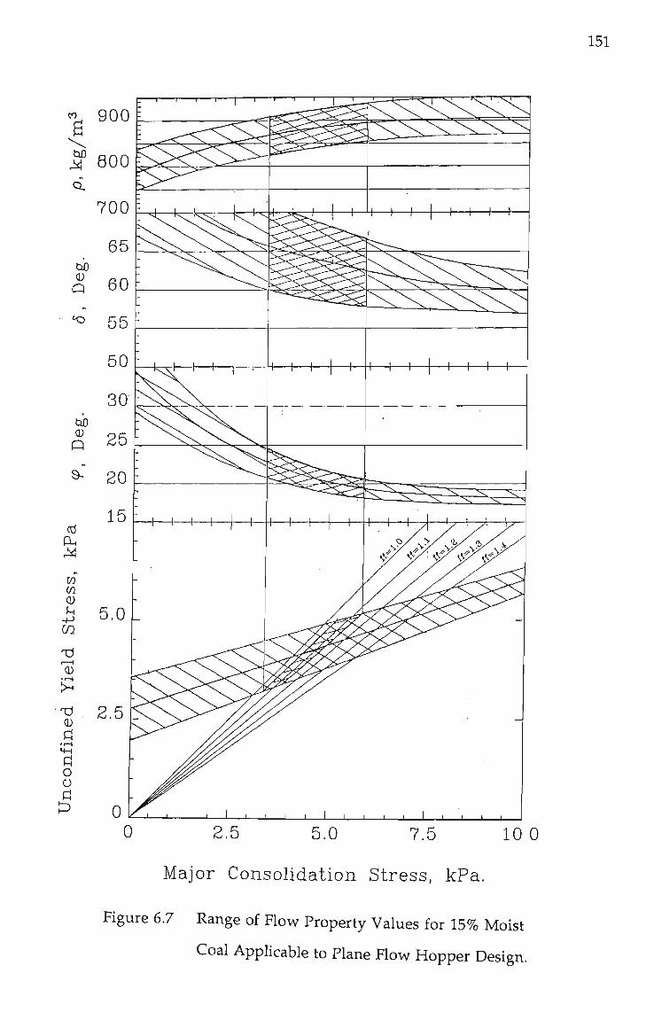
151

" 900

^ 800

10 0



Coal Applicable to Plane Flow Hopper Design.

152

Moisture Content Flow Factor Range

Axisymmetric Plane Flow

6%

10%

15%

1.11 <ff< 1.27

1.15 < ff < 1.25

1.15 <ff< 1.26

1.08 <ff< 1.18

1.06 <ff< 1.12

1.05 < ff < 1.14

Table 6.3: Range of Flow Factor Values at the Critical

Design Point for Axisymmetric and Plane Flow

Hoppers at Various Moisture Contents.

153

Comparison of the flow factor ranges indicates similar values for

both hopper types, with the axisymmetric case approximately 0.1 larger than

the plane flow value. The respective flow factor range for each case has been

used to graphically determine the critical G^ range from the intersection

with the flow function range. As indicated by the double hatched region in

Figure 6.2 to 6.7, the critical Oj exists in a narrow band.

Graphically projecting the minimum and maximum o^ values

onto the other flow properties allows the range of (j), 8 and p to be defined.

Comparison between Figures 6.2 and 6.7 show that for the same moisture

content, the axisymmetric case has lower 8 and (|) values due to the slightly

higher flow factor leading to higher values of Gy For increasing moisture

content, larger critical o^ values are evident due to the intersection of the

stronger flow functions with the relevant flow factors. The trend of larger a

values also leads to lower ^ values applicable for the 304-2B stainless steel.

An insight is gained into the variation of the hopper design

parameters (ff and a) by referring to Figures 6.8 to 6.9. These figures

represent an enlarged portion of the alternative hopper design parameter

charts onto which the values of ^ and 8 from the critical o^ range

determined in Figures 6.2 to 6.7 have been mapped. The curve within each

crosshatched region represents the variation of the mean values of 8 and ^,

as detailed in Figure 6.2 to 6.7.

Figure 6.8 (for axisymmetric hoppers) indicates that the flow factor

value is relatively insensitive to the sample moisture because the

inclination of the flow factor contours correspond to the trend of the

enclosed areas representing increasing moisture content. This observation

is not applicable to the plane flow case. Figure 6.9, because the flow factor

contours are approximately vertical. Both Figure 6.8 and 6.9 emphasise that

154

35

30 ^-^ 0

Q) 1—1

PI <1

C) •rH

-P crt III

ci) ^

•r-i

tiO (U

tt ^

on,

Jl

• r-l '^ ' - ' - fJ

o •rH !H

UH

1—1 1—1

^ 20

15 50 55 60 65 70

Effective Angle of In t e rna l Frict ion, 6 ,Deg,

Figure 6.8 Variation of 8 and <I>304_2B SS ^°^ Moist Coal (at

Various Moisture Contents) Mapped onto the

Alternative Axisymmetric Hopper Design

Parameter Chart.

155

50 55 60 65 70 Effective Angle of Internal Friction, (5 ,Deg.

Figure 6.9 Variation of 8 and (|)304_2B SS ^°^ Moist Coal (at

Various Moisture Contents) Mapped onto the

Alternative Plane Flow Hopper Design

Parameter Chart.

156

for both axisymmetric and plane flow hoppers, the hopper wall slope is

directly proportional to (j) and quite insensitive to 8, for 8: 50° < 8 < 70°.

Reviewing the trends presented by the figures in this chapter it is

proposed that the flow property testing of black coals for mass flow hopper

design can be significantly reduced without compromising the success and

reliability of the design. This can be achieved by utilising the charted values

(Figures 6.2 to 6.7) for the properties that have little influence on a and B

and testing those flow properties which have a significant effect. To expand

this hypothesis, first consider the determination of a and B. As previously

stated the outlet dimension is given by:

O j H ( a ) Oj H ( a )

B = = (TT) (1.2, repeated)

pg " pg

Rearranging and substituting Equations 5.5 and 5.6 for H(a), for

axisymmetric hoppers: a, (a + 130) OT (130+a)

B = = — (6.1) p 9.81x65 637.65p

and for plane flow hoppers:

G. (a + 200) G. (a+200) B = -^ =— (6.2)

p 9.81x200 1962p

Thus the primary variables of the above equations are Gy p and a.

An estimate of B can be determined by considering each of these variables.

The value of o^ is determined from the intersection between the flow

function and the relevant flow factor. As presented in Figures 6.2 to 6.7 for

various moisture contents and hopper types, the flow factor value range is

quite small, with a variation of approximately 0.1 for both axisymmetric and

plane flow outlets. However, considering the intersection with the range of

flow functions (X-G<X + G) the range of a^ is approximately 1.5 to 2 kPa.

This variation is obviously too large to utilise in the estimation of B.

157

The range of a^ can be reduced to an acceptable level by

experimentally determining one coordinate (Gy G^) of the flow function of

the bulk solid under consideration, such that G^ is positioned close to, or

within the a^ range of the double hatched intersection region for the

relevant moisture contents depicted in Figures 6.2 to 6.7. The flow function

can then be estimated, passing through (Gy GJ and with the slope of the

mean flow function. The value of o^ can then be determined from the

intersection between the estimated flow function and the relevant flow

factor range. The range G^ is given by the vertical difference of the

intersections with the minimum and maximum flow factors, and is

normally less than 0.25 kPa.

Utilisation of this approach, for black coals, allows the reduction

of the instantaneous yield loci test from three consolidation levels to one.

However, this alternative procedure, requires that the single yield locus

o^ be positioned close to the required a^ range, to minimise the error from

utilising the mean flow function slope in determining the intersection with

the relevant flow factor range. The determination of the consolidation level

for the single yield locus can be awkward due to the following aspects:

• determination of the required consolidation level for the yield

test due to the indirect method a^ is determined, from the Mohr

stress circle passing through the coordinates (V,S) and tangent to

the yield locus.

• the low values of o^ required. This is certainly the case for the 6%

moisture coals, and may require the use of aluminium shear cells

in preference to stainless steel, and coordinate levels of 21b rather

than the common lowest level of 31b.

Values of o^ required to provide maximum confidence should be

within the following ranges:

158

• 6%, a^: 1.5 < o^ <3.0 kPa

• 10%, Gj: 3.0 < o^ <5.0 kPa

• 15%, Gj: 3.5 < Oj < 6.0 kPa

For coals of different moisture contents to those presented, the

slope of the estimated flow function should be interpolated between the

trends of the known variations of 6%, 10% or 15% moisture content. This

alternative approach can also be used for the estimation of the hopper

outlet dimension for time consolidation at rest conditions. In a similar

manner to the instantaneous flow function, a single time yield locus would

be tested to provide one coordinate (Gy G^^) allowing the position of the time

flow function to be estimated. While no graphical trends for the time flow

function are provided, it is considered that sufficiently accurate values of o^

can be achieved using the slope of the respective mean instantaneous flow

function.

The intersection between the estimated flow function and the

flow factor range provides the range of a^ for the critical design point. This

value allows the range of bulk density to be found and utilised. As indicated

in Equation 6.1, an upper bound value of bulk density provides a

conservative calculation of the hopper outlet dimension.

The remaining parameter, a, influences Equation 6.1 to a minor

degree through the H(a) term. The significant influence of wall friction on

the determination of a has previously been highlighted. For this reason,

and the importance of correct selection of a to achieve mass flow,

experimental wall friction tests are considered mandatory. The

determination of ^ {ram. the wall yield locus, although involving 8, has a

minor influence and a point value of 8 estimated from Figure 6.2 to 6.7

would be adequate. The effect of 8 is only of primary consideration in

determining the minimum Gy for which the solution of ^ maximum *- ^ ^^

159

found. The determination of a from Figures 6.8 and 6.9, is straightforward

based on (j) (at the particular Oj estimated). On finding a. Equation 6.2 and 6.3

(for axisymmetric or plane flow hoppers respectively), can be determined to

yield estimates of the hopper outiet width.

The variation of <j) is also of primary concern in determining the

hopper geometry parameters for designs when the outlet dimension is

greater than the critical. This is particularly the case for wall materials that

display a reduction in (|) with increasing a^. The variation of allowable

hopper slope with outlet dimension can be determined by incrementing a^

and using the method described in Chapter 5.


This chapter details the development of guidelines based on two

approaches for the design of mass flow hoppers storing hard black coal. The

first considers the expected values of a and B represented by the mean of

each parameter within a 90% confidence interval. The values were

determined by analysing the hopper geometry parameter values

determined from the flow property testing program, by the Student's t

Distribution. The values of a and B provide the design engineer with

parameters which can be utilised at the layout stage, or when reviewing

existing hopper designs. The expected values highlight the steeper hopper

wall slopes required for coal at 6% moisture content and the larger outlet

dimensions required for the 10% and 15% moist coals. For the design of

facilities where the coal handled can have a range of moisture contents, this

feature should be recognised.

The second approach involved the development of a reduced

flow property testing program to determine/confirm those properties which

exert significant influence on the values of a and B, while for those

properties of less significance the expected values can be estimated from

160

charts. This approach stems from an analysis of the critical region of mass

flow hopper design, involving the flow properties of G^, 8, (1)304.23 ss ^^^ ^^^

relevant flow factor. The range of values for each flow property and the

design parameters a and ff have been presented graphically for coal at 6, 10

and 15% moisture content.

The influence of wall friction for the determination of a is most

significant. It is considered that the experimental wall friction test is

mandatory in achieving reliable mass flow hopper design. Even for those

situations where the outlet span is known from experience (or from shear

testing) the achievement of mass flow operation rather than the ratholing

characteristic of funnel flow is strongly dependent on the correct selection of

a, based on 0.

161

CHAPTER 7

APPLICATION OF COMPUTER AIDED DESIGN

TECHNIQUES

7.1 INTRODUCTION

The use of digital computers as a processing aid applied to bulk

materials handling has been recognised for some time, for example, the

work of Stainforth et al. [58], Budalli [59] and Eelkman Rooda [60].

From the initial work of Martin [61] and Dwight [62],

(undergraduate thesis topics. The University of WoUongong, supervised by

Dr. A.G. McLean), two computer programs have been developed that follow

the bin design procedure highlighted in Chapter 1.1. The first program, FP,

deals with the flow properties of the tested bulk solid, processing the

experimentally determined data and presenting the flow properties

graphically and by empirical equations. The second program, BD,

determines the mass flow hopper geometry parameters, at critical

conditions and calculates the design chart of variation of hopper slope with

increasing outlet dimension. The two programs are linked, in that the

empirical flow property equations determined by the first program are used

as the data input into the hopper design program.

features.

Development of the programs has incorporated two important

A high degree of operator interactive control. This allows a

greater flexibility and freedom in selecting the required program

option and on completion returning the operator to the main or

root menu for the next selection.

162

• The utilisation of high resolution graphics which has brought

advantages in providing a convenient method of checking

experimental data, checking and accepting experimental curve

regressions and interpreting hopper design graphs.

The software was initially developed within the The University

of WoUongong Computer System environment. This is a time-share

system based on a UNIVAC 1100/80 mainframe computer, with FORTRAN

as the primary programming language. The version of FORTRAN used is

SPERRY-UNIVAC FORTRAN 77 (conforming to ANSI Standard X3.9-1978).

While these programs have been developed specifically for the University

system, using on-line packages such as the PLOT PACKAGE [63]and IMSL

[64] their philosophy and program logic is applicable generally.

It has been recognised for some time that access to these programs

was limited due to program operation only being available on the

mainframe system. To allow wider exposure, particularly in view of the

widespread use of powerful engineering design microcomputers, both

programs have been transferred to a microcomputer design system within

the Department of Mechanical Engineering.

7.2 MICROCOMPUTER DESIGN SYSTEM

Plate 7.1 presents an overall view of the microcomputer design

system. The microcomputer is a Sperry IT Personal Computer, based on a

80286 microprocessor with 80287 numeric co-processor. The system has been

configured in a dual display mode. That is, one monitor is dedicated to text

display, and the larger monitor displays all graphics output. This

configuration is well suited to the processing and analysis of the

experimental flow properties because data points may be edited via the text

monitor while viewing the graphical presentation on the adjacent display.

Plate 7.2 presents a view of both displays to highlight this feature. In a

163

Plate 7.1: View of the Microcomputer Design System.

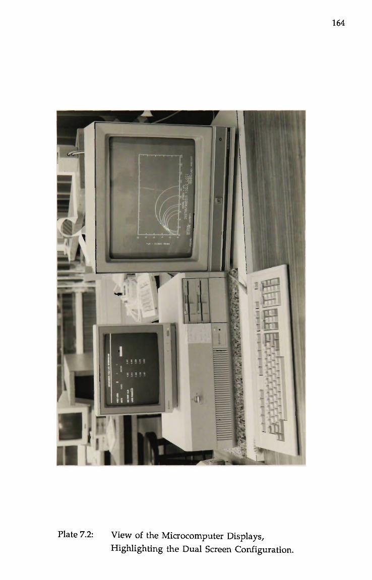
164

Plate 7.2: View of the Microcomputer Displays,

HighHghting the Dual Screen Configuration.

165

single monitor configuration the operator would need to switch

alternatively between text and graphics modes in using this software.

Enhancements to this Sperry computer include 1.2 megabyte and

360 kilobyte floppy disc drives, 40 megabyte hard disc drive, 2 megabyte

extended memory (often termed virtual disk), and one parallel and two

serial communication ports. Computer periphercds (presented in Plate 7.1)

include a NEC P7 Pinwriter printer for producing typed reports and a

Mutoh IP-500 multi-pen plotter for the plotting of flow property graphs and

hopper design graphs.

Graphical output is achieved by a Vectrix VX/PC Graphics card

(developed by Vectrix Corporation, USA) and displayed on the Electrohome

D03 Series 19" RGB colour monitor. Features of the graphics card include a

high level graphics command language, a screen resolution of 672 x 480

pixels with 4096 possible colours and nine bitplanes.

The programs developed for the microcomputer operate within

the MS-DOS operating environment. They are programmed in FORTRAN

and compiled by the F77L FORTRAN compiler (licensed product from

Lahey Computer Systems Inc., USA.). This compiler was selected because it

was considered to be the closest aligned to the ANSI FORTRAN Standard

X3.9-1978, and, compared to other compilers, had superior speed in terms of

execution time and features such as an on-line debugging and subroutines

for DOS system access. Linking or mapping of the compiled machine code

into executable programs was achieved using PLINK 86 , (licensed product

from Phoenix Technologies Ltd. USA.). Features of this linker include

complex code overlay management for RAM swapping and the ability to

form compiled libraries of code.

166

The data input and output from the microcomputer programs is

an important aspect. Data file access within MS-DOS has been incorporated

allowing read/write operations to files in branched directories or sub

directories existing on the hard disk or floppy disks. Thus, for subsequent

executions of a program, the data does not need to be retyped, but only the

data file directory location specified. Output files which store processed

report summaries for printing, and graphic data files for plotting are

generated automatically by the programs. These features will be highlighted

in the respective discussions of each program.

Communication with the Vectrix Card for graphical output was

achieved using a University developed FORTRAN PLOT PACICAGE [63]

transferred and recompiled on the microcomputer. The graphic command

strings are post-processed to convert the code into HP-GL, (Hewlett-Packard

Graphics Language), which is required for controlling the Mutoh plotter.

Background plotting of graphics is achieved by using the memory resident

utility program AutoPLOT II (licensed product from DSL Inc., USA.). This

allows the operator to be executing one of the bulk materials programs

while the microcomputer is also communicating graphics commands to the

plotter.

Incorporation of user-friendly aspects in the development of both

programs for the microcomputer system has received a high priority.

Features include:

• a full screen editor for interactive data input/adjustment

• a hierarchical menu structure where repeated ESC keystrokes will

return the operator from any module branch to the root menu.

• extensive use of the ANSI Escape sequences for formatting of the

text monitor with controlled cursor positioning and highlighted

text. Advanced keyboard read sequences also allow single

167

keystroke responses to option selections (rather than requiring an

additional RETURN keystroke).

• default responses supplied for many of the option selections.

• An interactively controlled information page facility to aid

operator familiarisation of the program structure and execution.

The complete FORTRAN computer code of both programs has

not been included in the Appendix because of the large amount of code.

However, interested readers are invited to contact the author should they

require further detailed information.

Each computer program will now be considered in detail. As the

development of the programs for the microcomputer was the most recent,

details and features relate particularly to this system.

7.3 COMPUTER PROCESSING AND ANALYSIS OF THE FLOW

PROPERTIES OF BULK SOLIDS; PROGRAM FP

The program FP allows the rapid processing and analysis of the

considerable amounts of experimental data obtained from the flow property

testing of the bulk solid materials. The interactive format of the program

has particular advantages in the processing of experimental data, since

editing features and the graphical output displays allow the adjustment of

doubtful points, and analysis of the data can be repeated until satisfactory,

within the same program execution session. The presentation of the flow

property results graphically has provided an invaluable aid in highlighting

doubtful data points. It also provides a quick and convenient means of

obtaining permanent copies of the flow property variations by means of the

Mutoh IP-500 plotter.

168

In addition to providing the graphical output, each of the flow

properties are described by an empiriccil equation that is curve-fitted to the

relevant data by various regression techniques.

The FP program consists of 6,868 lines of FORTRAN code

arranged in 38 symboHc files (excluding the PLOT PACICAGE and IMSL

routines). Appendix Ll presents a summary of the size (bytes) and number

of lines of each file. The size of the executable file FP.EXE is 448 kilobytes.

Figure 7.1 presents a flow chart of FP at the root menu level. It can be seen

that maximum flexibility has been provided in being able to select the

required options, and on completion of the task, return to this root menu.

The code listing of FPMAIN.FOR, the main calling program which controls

the root menu is provided in Appendix 1.2. There are substantial menus of

lower hierarchical status from each of the major options. These control

such features as data input and editing functions, graphical display options

and engineering units.

It is not intended to provide a full discussion of the laboratory

procedures involved in the flow property testing. These have been fully

documented in References [3,4] and discussed in Chapter 2. Before

presenting a detailed description of each major option, the characteristic

empirical equations (and the procedures in determining the parameter

values) used in describing the respective flow properties will be discussed.

7.3.1 Representation of Flow Properties by Empirical Equations

To allow subsequent computer programs, such as the bin design

program, BD, to utilise iterative design procedures based on the bulk solid

flow properties, they must be described by empirical equations. These

continuous functions allow the bin design program to calculate the critical

design values with greater accuracy and speed than by considering discrete

point values representing the flow property variations. Table 7.1 presents a

169

C start 3

Enter Data Filenames and Bulk Solid Material Details,

V J

Select Flow Property Option from the Root Menu: ESC : Finish Program

Fl : Instantaneous Yield Locus and Flow Function

F2 : Time Yield Locus and Time Flow Function

F3 : Wall Yield Locus

F4 : Kinematic Angle of Wall Friction

F5 : Bulk Density Variation

Fl r Low and High Pressure Instantaneous Yield Loci

Present Resulting Flow Function and/or Extended Flow Function Present Variations of d with Consolidation Stress Fit Empirical Equations to Flow Functions and d Variations

F2 - Low and High Pressure Time Yield Loci - Present Resulting Time Flow Function and /or Extended Time

Flow Functions, including Previous Instantaneous Flow Function - Present Variation of ft with Consolidation Stress - Fit Empirical Equations to Flow Functions and ft Variation

F3 - Wall Yield Loci for a Limit of 10 Wall Lining Materials - Fit Empirical Equations to Describe the Wall Yield Loci }

F4 - Present the Kinematic Angle of Wall Friction Variation with Consolidation Stress, for a Limit of 10 Wall Lirung Materials }

F5 - Present the Variation of Bulk Density Variation with Consolidation Stress in Linear and Logarithmic Graphical Formats

- Fit the Empirical Equation to Describe the Bulk Density Variation

Figure 7.1: Flow Chart of Computer Program FP.

170

Instantaneous Flow Function:

G = 0.400^ + 0.63 c 1

2 Day Time Flow Function:

G^ = 0.42O, + 0.95 c t Jl

Effective Angle of Internal Friction Variation: 1964.28

8 = 16.71 + 33.66 + Oj

Static Angle of Internal Friction Variation:

(t)j = O.OlOj + 35.10

Bulk Density Variation:

rrorr -, A , _ ^ 1 v0.0767

P = 787.14 (^^)

Wall Yield Locus Equations

Rusty Mild Steel:

t = 51.78 4195.07

81.25 + G

304-2B Stainless Steel:

T = 0.25a + 0.37

Table 7.1: Typical Empirical Flow Property Equations

171

typical set of empirical equations representing the flow properties of moist

coal determined by FP.

The flow properties of the instantaneous and time flow functions,

effective angle of internal friction, static angle of internal friction and the

wall yield loci can be adequately described by either:

• a straight line (form Y = m X + b )

• a three parameter equation originally suggested by Johanson and B

Carson [65]. This equation has the form Y = A - /p ^x where A, B

and C are constants.

The three parameter equation is advantageous for computer

applications in being able to represent flow properties of both concave and

convex forms by suitable selection of the signs and relative values of each of

the constants. Considering the three parameter equation further, the

following aspects are important:

• as X => oo, Y => A, with an asymptotic variation. B

• for X = 0, the Y intercept is Y = A - p

• for a positive B, the three parameter variation is convex upward.

However, for a negative B, the equation form becomes B

Y = A - /p wy and the variation is concave downward. This

second form is particularly useful for curve fitting the effective

angle of internal friction variation.

• the rate of decay is dependent on the relative absolute values of B

andC.

The variation of bulk density with major consolidation stress is

adequately described by a power equation of the form p = PQ(—) • It will be o

realised that using log format, this relation gives a straight line with a

172

a gradient of 'b' and passing through the centroid of the experimental data

The two equation forms (linear or three parameter) are

curve-fitted to the experimental data by implementing one of the following

regression techniques:

• least squares regression,

• constrained Rosenbrock Hillclimb [66],

• unconstrained Fletcher-Powell optimisation [66].

Acceptance of a particular equation is based on a visual acceptance

of the graphical output. A characteristic of the optimisation techniques,

particularly the constrained Rosenbrock method is the dependence of the

optimised solution on the initial starting points selected. As a result a

starting point algorithm has been developed to allow the user to select

suitable starting points or allow these to be selected with regard to certain

ratios [61]. The constrained Rosenbrock Hillclimb is required for particular

flow properties, to overide the experimental data if necessary. Such cases

include:

• Constraining the flow functions, wall yield loci and the static

angle of internal friction to have a convex upward variation.

• Constraining the flow functions to pass through the origin if a

positive abscissa (X-axis) intercept occurs.

• Constraining the effective angle of internal friction to a concave

downward variation. Additional constraints force a positive

ordinate intercept maximum limit of 80 . A straight line will be

curve fitted if the data actually presents a convex upward

variation.

173

Several shortcomings found with the use of the Rosenbrock

method (particularly in terms of computation time) were ehminated by

implementing the Fletcher-Powell method, which, while not providing a

constrained solution, is more flexible with regard to starting points and

speed of convergence.

7.3.2 Execution of Program FP

The operation and features of this program is best highlighted by

an example, and a ROM coal at 10% moisture content will be used for this

purpose. Printouts of the text monitor screen are presented with this

discussion to illustrate the operator/program interaction for the various

options.

On starting the program by typing \FP\FP, and loading of the

code into memory, the text screen displays the titiepage. Figure 7.2. The

initial considerations of the program are the data file input and output

operations. For efficient system management and recording the results of

each execution session, FP can be executed from the operator's personal MS-

DOS directory, rather than the root directory. This approach ensures that for

several operators the respective data files (which can be custom named) will

reside in the directory of the operator and not be liable to corruption or

erasure by other users.

On leaving the titiepage, the bulk solid characteristics are entered

through the display depicted in Figure 7.3. The details entered will be later

appended to each of the graphical presentations, as part of the titleblock. As

indicated in Figure 7.3, the uppermost three lines of each text screen

contains a status bar to inform the user of the current location in the

program or option.

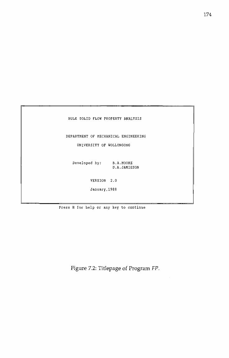
BULK SOLID FLOW PROPERTY ANALYSIS

DEPARTMENT OF MECHANICAL ENGINEERING

UNIVERSITY OF WOLLONGONG

174

Developed by: B.A.MOORE D.A.JAMIESON

VERSION 2.0

January,1988

Press H for help or any key to continue

Figure 7.2: Titiepage of Program FP.

BULK SOLID CHARACTERISTICS

ENTER MATERIAL DATA AS REQUESTED

MATERIAL TESTED: RUN OF MINE COAL

MOISTURE CONTENT: 10% Nom.

DATE TESTED: JANUARY,1988

TEMPERATURE <AMBIENT>:

Figure 7.3: Enh-y of Bulk Solid Characteristics.

REPORT FILE ASSIGNMENT

PROCESSED DATA STORAGE FILE (REPORT): ROM-REP

PLOT STORAGE FILES CODE NAME <FP>: ROM-P

Figure 7.4: Setup of Data Output Files.

175

176

Two major output data files are involved in the program

operation. As presented in Figure 7.4, the first file contains the processed

flow property data and empirical equations arranged in a report format,

(Appendix 1.3 presents the report processed from the example). The second

data file stores graphical displays selected by the operator for plotting during

or after the current execution session. As indicated specific file names may

be entered, otherwise the default names are used by responding with a

RETURN keystroke.

This completes the initial information required by FP, and the

root menu of the program is then displayed (Figure 7.5). Option selection is

achieved by using the programmable function keys provided on most IBM-

PC compatible computer keyboards. Pressing ESC terminates the program

execution.

The operation and features of the various options will now be

presented based on a set of experimentally determined flow property data

from the coal testing program.

7.3.3 Instantaneous Yield Locus

The basic flow property test is the determination of the family of

instantaneous yield loci using the standardised procedure presented in

Appendix A. The shear strength is determined under various normal

stresses at normally three consolidating pressures to produce the family of

yield loci. For each yield locus, two Mohr circles of stress can be drawn

tangential to the locus: one passing through the origin defining the

unconfined yield stress (G ) and the second, passing through the steady state

shear co-ordinates, determining the major consolidation stress (a^).

177

FLOW PROPERTY TESTS AVAILABLE

WHICH FLOW PROPERTY TEST DO YOU REQUIRE TO PROCESS

ESC - FINISH Fl - INSTANTANEOUS YIELD LOCI AND FLOW FUNCTION F2 - TIME YIELD LOCI AND FLOW FUNCTIONS F3 - WALL YIELD LOCI F4 - KINEMATIC ANGLE OF WALL FRICTION VARIATION F5 - BULK DENSITY VARIATION

OPTION

Figure 7.5: Root Menu of Program FP.

178

Several researchers have considered the yield loci to be convex

upward and to be adequately described by the so-called Warren-Spring

equation [58]: r'^ ^T\. o [-]=j + l (7.1)

where c, n, and T are constant.

Experience has shown that the yield loci can be conveniently

represented by straight line segments. By comparison with the convex yield

loci, this approach generally produces larger values for the unconfined

stress (G^) and hence more conservative design data. The straight line

representation has the advantage of leading to simplified mathematical

relations to determine:

•the effective angle of internal friction

•the unconfined yield stress

• the major consolidation stress.

It is essential that this computer program be regarded as an aid to

producing graphical representations of the yield loci and not as a

replacement for the hand drawn graph which must be obtained during the

course of shear testing in the laboratory. To allow the correct interpretation

on the experimental data the observations and valid ranges detailed in

Appendix A.5 and Figure A.4 must be adhered to.

Figure 7.6 presents the first text screen of option Fl, for the data

entry of the instantaneous yield loci from either the keyboard or data file. If

the keyboard entry approach is selected the program first prompts for a

filename to store the experimental values (to allow data file entry for

subsequent program runs) and then displays Figure 7.7 for the input of data

for each consolidation level. For this text screen, cursor positioning adjacent

to each respective text string occurs allowing rapid and convenient data

179

INSTANTANEOUS YIELD LOCI DETERMINATION

DATA ENTRY METHOD:

Fl - KEYBOARD F2 - DATA FILE

OPTION

OUTPUT FILE <.DAT> ROM-IYL.DAT

ARE THE UNITS IN 0:POUNDS, 1:NEWTONS OR 2:KIL0PASCALS 0

NUMBER OF YIELD LOCI 3

Figure 7.6: Data Input of Experimental Values into the Instantaneous Yield Loci Module.

180


YIELD LOCUS 1:

END POINT OF YIELD LOCUS (V,S) 7.84 8.05

NUMBER OF POINTS ON YIELD LOCUS 4

ENTER YIELD LOCUS POINTS (NORMAL FORCE,SHEAR FORCE) 4.84 6.3 3.84 5.5 3.34 5.1 2.84 4.7

YIELD LOCUS 2:



ENTER YIELD LOCUS POINTS (NORMAL FORCE,SHEAR FORCE) 3.83 5.06 3.33 4.71 2.83 4.33 2.33 3.83

YIELD LOCUS 3:



ENTER YIELD LOCUS POINTS (NORMAL FORCE,SHEAR FORCE) 2.32 3.4 2.07 3.1 1.82 2.92

Figure 7J: Text Screen Arrangement for Data Input into

the Instantaneous Yield Lod Module.

181

entry. The program caters for a maximum of five consolidation levels each

consisting of six yield lod coordinates. The program provides checks on the

data to ensure the yield locus fitted does not lie below the shear

consolidation value (V,S) or have a negative cohesion value (C, Figure A.4).

On completion of the data entry, an intermediate menu is

displayed, allowing the user to return to the root menu, edit data for typing

errors or display graphs of the instantaneous yield loci. Option F4 eillows the

instantaneous flow function to be superimposed over the instantaneous

yield loci. Figure 7.8 presents a typical display for this option, which has

proved useful in checking of experimental yield loci data.

At the completion of the plot (displayed on the graphics monitor)

the text screen displays the main menu for the instantaneous yield loci

options, presented in Figure 7.9. As indicated the important parameters of

G., G and 8 are tabulated for each consolidation level. 1' c

No facility has been provided in the program for automatically

weighting individual data points. However, in determining the family of

instantaneous yield loci, it is often necessary to shift slightly the shear

values associated with individual data points as the computer program

treats each yield locus individually. An editing option, Fl, allows this

manual adjustment of the data points. Figure 7.10 presents the text screen

format of this option. The editor has a full screen format, meaning that the

complete yield data for each consolidation level is displayed and individual

normal or shear data values can be edited separately, rather than retyping

the complete coordinate. The YIELD LOCUS and UNITS status lines allow

the different data formats to be selected by positioning the cursor on the

relevant option. For instance, the yield loci data can easily be edited in

either pounds of kilopascals by selecting the required term in the UNITS

status line.

182

o CL

cn (n UJ CC I -cn

EC CC

i :

NORMAL STRESS - kPa

INSTflNTRNEOUS YIELD LOCI Mfl lERIRL: RUN OF MINE CORL TESTED: JflNUflRT.1988 MOISTURE CONTENT: 107. Nom. TEMPERRTURE: AMBIENT

Figure 7.8: Instantaneous Flow Function Superimposed

over the Instantaneous Yield Loci.


FLOW FUNCTION DATA SIGMAKkPa) SIGMAC(kPa)

11.88 6.29 8.99 5.18 5.71 3.77

DELTA(Degree) PHI(Degree) 53.51 55.57 59.64

38,66 39.15 40.03

SELECT REQUIRED OPTION

ESC Fl F2 F3 F4 F5 F6 F7

OPTION

RETURN TO MAIN MENU EDIT YIELD LOCI DATA CALCULATE PARAMETER TABLE, WITHOUT PLOT DISPLAY PLOT PLOT WITH FLOW FUNCTION DISPLAY VI AND F IN POUNDS CURVE FIT AND PLOT FLOW FUNCTION PROCESS HIGH PRESSURE YIELD LOCI DATA

Figure 7.9: Main Menu of the Instantaneous Yield Loci

Module.

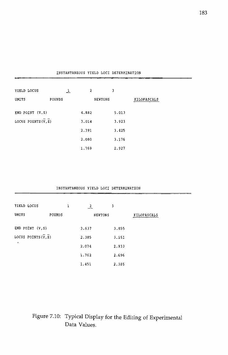
183


YIELD LOCUS

UNITS POUNDS

END POINT (V,S)

LOCUS POINTS{V,S)

J 2

4.882

3.014

2.391

2.080

1.769

NEWTONS

3

5.013

3.923

3.425

3.176

2.927

KILOPASCALS


YIELD LOCUS 1

UNITS POUNDS

END POINT {V,S)

LOCUS POINTS(V,S)

Jl

_2_

3.637

2.385

2.074

1.762

1.451

NEWTONS

3

3.855

3.151

2.933

2.696

2.385

KILOPASCALS

Figure 7.10: Typical Display for the Editing of Experunental Data Values.

184

Figure 7.11 presents the final instantaneous yield loci graph

processed for the example. Note that the graphical axes are automatically

scaled to produce the clearest and most convenient presentation of the data.

On pressing ESC the user is returned to the root menu and the

respective values of Gy G^ and 8 for each consolidation level are stored for

later presentations.

7.3.4 Time Yield Loci

The gain in strength of the bulk solid due to time storage at rest

may be assessed by considering the family of time yield lod. These lod also

conform to the observations listed in Appendix A.5, with the additional

observation that is unusual for the values of o . to be less than G . If this ct c

occurs it usually indicates erroneous experimental data.

The data entry section of the time yield loci module is similar to

that of the previous instantaneous yield loci option except that the period of

time consolidation is also entered, and the data for each consolidation level

is linked to the previously entered instantaneous data.

On completion of the data input, the values of Gy G^^ and ^^^ are

tabulated for each consolidation level (Figure 7.12). To aid the adjustment of

the time yield loci, option F4 allows the instantaneous flow function and

the time flow function to be superimposed over the time yield loci

currently being processed. This allows the time yield loci to be checked

indirectly by comparison of the data points (Gy G^^) against the instantaneous

flow function as indicated in Figure 7.13. Data can be adjusted if required

using the same editing facilities as the instantaneous yield loci module.

Figure 7.14 presents the final time yield loci graph.

On exit from this module the values of a ^ and ^^ for respective

values of CT^ are stored for later presentations.

10

tn UJ

I -

a: cn LU r cn

185

8. • T t 1 "I I I I t 1 XI T - T T - p i r 1 'T T I I [ I r I I I I I I I [ J l~T" T T-T I » I t -F I

• • • I • • • ' ' • • *

14. 16. NORMRL STRESS - kPo

INSTRNTRNEOUS YIELD LOCI MRTERIRL: RUN OF MINE CORL TESTED: JRNUflRT,1988 MOISTURE CONTENT: 10% Nom. TEMPERRTURE: RMBIENT

Figure 7.11: Typical Instantaneous Yield Loci Plot.

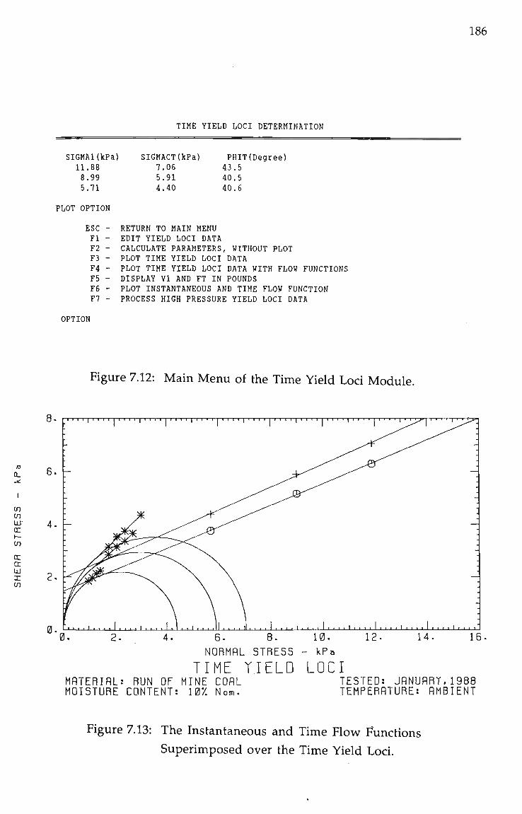
186

TIME YIELD LOCI DETERMINATION

SIGMAKkPa) 11.88 8.99 5.71

PLOT OPTION

ESC -Fl -F2 -F3 -F4 -F5 -F6 -F7 -

SIGMACT(kPa) 7.06 6.91 4.40

PHIT(Degree) 43.5 40.5 40.6

RETURN TO MAIN MENU EDIT YIELD LOCI DATA CALCULATE PARAMETERS, WITHOUT PLOT PLOT TIME YIELD LOCI DATA PLOT TIME YIELD LOCI DATA WITH FLOW FUNCTIONS DISPLAY VI AND FT IN POUNDS PLOT INSTANTANEOUS AND TIME FLOW FUNCTION PROCESS HIGH PRESSURE YIELD LOCI DATA

OPTION

Figure 7.12: Main Menu of tiie Time Yield Loci Module.

Q_

tn tn UJ

az

cn QI •cr Ui X tn

I I I I I I I I I I I 1 I I I I I I I I I I I r 1 I I I I I I I I T 1 I I I I 1 I I I I I > j I I r I I I I I I I I 1 I I I I I I 1 ^

0. 4. 6. 8. 10. NORMRL STRESS - kPa

TIME YIELD LOCI MRTERIRL: RUN OF MINE CORL TESTED: JRNURRT,1988 MOISTURE CONTENT: 107. Nom- TEMPERRTURE: AMBIENT

Figure 7.13: The Instantaneous and Time Flow Functions

Superimposed over the Time Yield Loci.

187

c

tn tn UJ

a: H CQ a: cn UJ r in

I I I I ,1 I I I I I I I I I I < I I I I I I I I ,| M I I I 1 I I I I I I I I I I I I I I I I I I I I I I I I I I I I

CONSOLIDRTIGN TIME:3 Days

I r t I I ' ' ' ' I ' ' ' ' ' ' ' ' ' ' ' ' ' '

4. 5. 6. 7. 8. 9. 10. 11. 12. NORMRL STRESS - kPa

TIME YIELD LOCI MRTERIRL: RUN OF MINE CORL TESTED: JflNURRT,1988 MOISTURE CONTENT: 107. Nom- TEMPERRTURE: AMBIENT

Figure 7.14: Typical Time Yield Loci Plot.

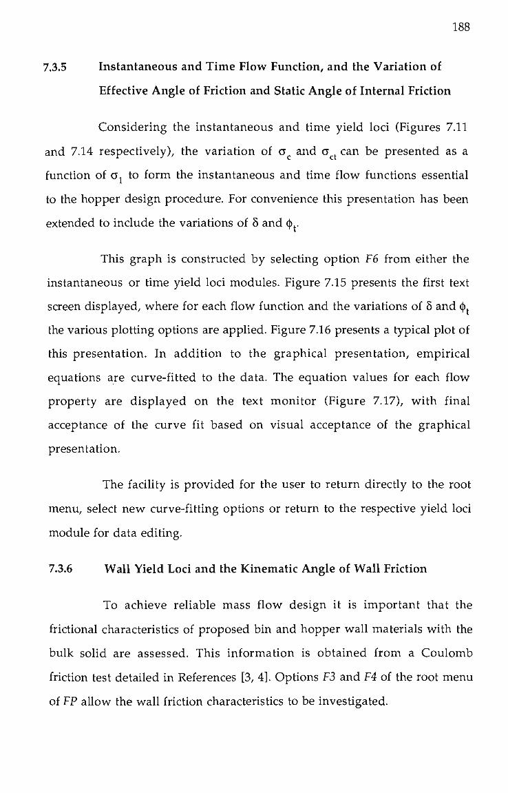
188

7.3.5 Instantaneous and Time Flow Function, and the Variation of

Effective Angle of Friction and Static Angle of Internal Friction

Considering the instantaneous and time yield loci (Figures 7.11

and 7.14 respectively), the variation of o^ and G^^ can be presented as a

function of o^ to form the instantaneous and time flow functions essential

to the hopper design procedure. For convenience this presentation has been

extended to include the variations of 8 and ^^.

This graph is constructed by selecting option F6 from either the

instantaneous or time yield loci modules. Figure 7.15 presents the first text

screen displayed, where for each flow function and the variations of 8 and ^

the various plotting options are applied. Figure 7.16 presents a typical plot of

this presentation. In addition to the graphical presentation, empirical

equations are curve-fitted to the data. The equation values for each flow

property are displayed on the text monitor (Figure 7.17), with final

acceptance of the curve fit based on visual acceptance of the graphical

presentation.

The facility is provided for the user to return directly to the root

menu, select new curve-fitting options or return to the respective yield loci

module for data editing.

7.3.6 Wall Yield Loci and the Kinematic Angle of Wall Friction

To achieve reliable mass flow design it is important that the

frictional characteristics of proposed bin and hopper wall materials with the

bulk solid are assessed. This information is obtained from a Coulomb

friction test detailed in References [3, 41. Options F3 and F4 of the root menu

of FP allow the wall friction characteristics to be investigated.

189

FLOW FUNCTION & FRICTION ANGLE VARIATIONS

INSTANTANEOUS FLOW FUNCTION PLOT OPTION

ENTER YOUR CHOICE FOR EACH SET OF DATA

ESC - OMIT FLOW PROPERTY FROM PLOT Fl - PLOT DATA POINTS ONLY F2 - PLOT STRAIGHT LINE EQUATION F3 - PLOT THREE PARAMETER EQUATION

OPTION

EFFECTIVE ANGLE OF FRICTION PLOT OPTION



OPTION

STATIC ANGLE OF INTERNAL FRICTION PLOT OPTION



OPTION

PLOTTING OPTION

ESC - BY-PASS PLOT Fl - DISPLAY PLOT

OPTION

Figure 7.15: Selection of Curve-Fitting and Plotting Options within the Flow Function Module.

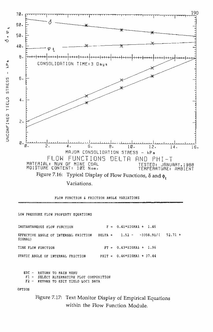
a a.

tn tn UJ OC I -tn

a _ J UJ

Q UJ

u. z o u

7 0 . [ _ ' ' ' ' I ' ' ' ' I ' ' I ' I ' ' ' ' I ' ' ' ' ] ' • ' ' I • ' ' 11 ' ' ' ' I ' I • ' I I • 11

60. E-

50.

40.

8.

4. -

190 I ' ' ' ' I ' ' I ' 1 1 1 1 1 1 1 1 1 1 1 1 1 1 1 •

Vi -X- • X -

JK—

" I ' I " n I n I I I I 11 I [ I I I 11 I I 11 I I I I I I 11 I I I 11 I I I I 11 1 I I I 11 I I I I I I I I 11 I M>[ I I 111 I i i >

CONSOLIDRTIGN TIME:3 Days

. . . . I ' ' ' I ' I I I ' I ' I I I ' ' I I I I ' ' ' I ' ' ' ' ' I ' • . ' ' • • . • ' • • • . ' • . • • I • • • • I • • • • I -LL.

14. 0- 2. 4. 6. 8. 10. 12. MRJGR CGNSGLIORTIGN STRESS - kPa

FLON FUNCTIONS DELTA AND PHI-T MRTERIRL: RUN OF MINE CGRL TESTED: JRNURRr.1988 MOISTURE CONTENT: 107. Nom. TEMPERRTURE: RMBIENT

Figure 7.16: Typical Display of Flow Functions, 8 and (|).

Variations.

16.

FLOW FUNCTION & FRICTION ANGLE VARIATIONS

LOW PRESSURE FLOW PROPERTY EQUATIONS

INSTANTANEOUS FLOW FUNCTION F =

EFFECTIVE ANGLE OF INTERNAL FRICTION DELTA SIGMAl)

TIME FLOW FUNCTION FT

STATIC ANGLE OF INTERNAL FRICTION PHIT

0.41*SIGMA1 + 1.46

1.52 - -3358.91/( 52.71 +

0.43*SIGMA1 + 1.96

0.46*SIGMA1 + 37.44

ESC - RETURN TO MAIN MENU Fl - SELECT ALTERNATIVE PLOT COMPOSITION F2 - RETURN TO EDIT YIELD LOCI DATA

OPTION

Figure 7.17: Text Monitor Display of Empirical Equations

within the Flow Function Module.

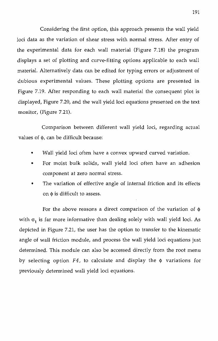
191

Considering the first option, this approach presents the wall yield

loci data as the variation of shear stress with normal stress. After entry of

the experimental data for each wall material (Figure 7.18) the program

displays a set of plotting and curve-fitting options applicable to each wall

material. Alternatively data can be edited for typing errors or adjustment of

dubious experimental values. These plotting options are presented in

Figure 7.19. After responding to each wall material the consequent plot is

displayed. Figure 7.20, and the wall yield loci equations presented on the text

monitor, (Figure 7.21).

Comparison between different wall yield loci, regarding actual

values of ^, can be difficult because:

• Wall yield loci often have a convex upward curved variation.

• For moist bulk solids, wall yield loci often have an adhesion

component at zero normal stress.

• The variation of effective angle of internal friction and its effects

on ^ is difficult to assess.

For the above reasons a direct comparison of the variation of 0

with G^ is far more informative than dealing solely with wall yield loci. As

depicted in Figure 7.21, the user has the option to transfer to the kinematic

angle of wall friction module, and process the wall yield loci equations just

determined. This module can also be accessed directly from the root menu

by selecting option F4, to calculate and display the (j) variations for

previously determined wall yield loci equations.

192

WALL YIELD LOCI

WALL MATERIAL TESTED: RUSTY MILD STEEL

IS THE DATA IN 0:POUNDS, 1:NEWTONS OR 2:KILOPASCALS: 0

NUMBER OF POINTS ON WALL YIELD LOCUS: 10

ENTER WALL YIELD LOCUS POINTS (NORMAL FORCE,SHEAR FORCE)

0.81 0.6 2.81 2.1 4.81 3.4 6.81 4.6 8.81 5.5 10.81 6.98 12,81 7.96 14.81 8.73 16.81 10.08 18.81 11.0

WALL MATERIAL TESTED: PACTENE




0.81 0.54 2.81 1.29 4.81 2.0 6.81 2.64 8.81 3.38 10.81 4.03 12.81 4.65 14.81 5.48 16.81 6.23 18.81 6.99

WALL MATERIAL TESTED: 304-2B STAINLESS STEEL




0.81 0.72 2.81 1.35 4.81 1.94 6.81 2.55 8.81 3.12 10.81 3.68 12.81 4.2 14.81 4.8 16.81 5.36 18.81 5.82

Figure 7.18: Enh-y of Experimental Wall Yield Lod Data.

193

WALL YIELD LOCI

PLOT OPTION FOR EACH WALL MATERIAL

ESC - OMIT FROM PLOT Fl - PLOT DATA POINTS ONLY F2 - PLOT STRAIGHT LINE EQUATION F3 - PLOT THREE PARAMETER EQUATION (CONSTRAINED) F4 - PLOT THREE PARAMETER EQUATION (UNCONSTRAINED) F5 - TO MODIFY DATA

RUSTY MILD STEEL

WALL YIELD LOCI

PLOT OPTION FOR EACH WALL MATERIAL

ESC - OMIT FROM PLOT Fl - PLOT DATA POINTS ONLY F2 - PLOT STRAIGHT LINE EQUATION F3 - PLOT THREE PARAMETER EQUATION (CONSTRAINED) F4 - PLOT THREE PARAMETER EQUATION (UNCONSTRAINED) F5 - TO MODIFY DATA

304-2B STAINLESS STEEL

Figure 7.19: Selection of Curve-Fitting and Plotting Options

within the Wall Yield Option.

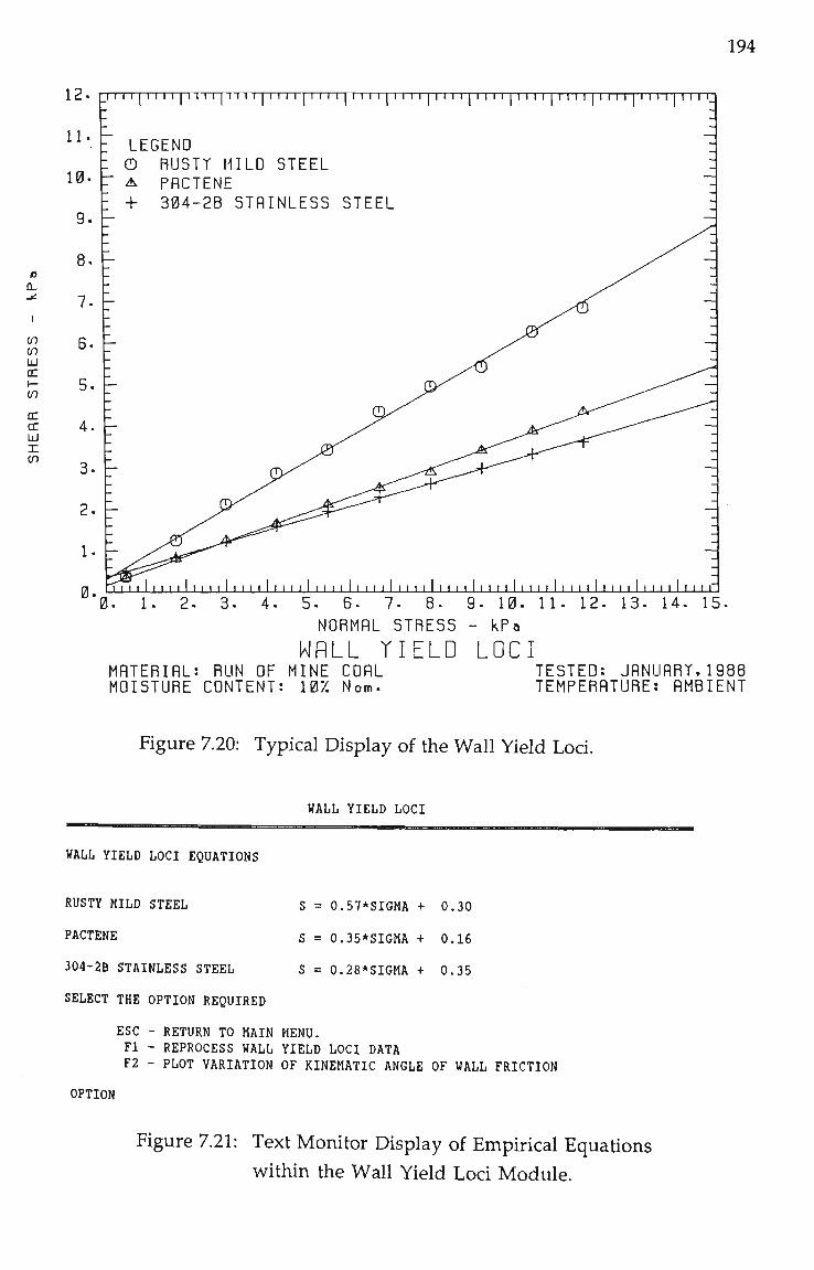
194

o

<n tn u a: h-(n

CC cr UJ X tn

0. 1. 2. 3- 4. 5. 6. 7. 8. 9. 10. 11. 12- 13. 14. 15. NORMRL STRESS - kPa

WALL YIELD LOCI MRTERIRL: RUN OF MINE CORL TESTED: JRNUflRT,1988 MOISTURE CONTENT: 10"/ Nom- TEMPERATURE: RMBIENT

Figure 7.20: Typical Display of the Wall Yield Lod.

WALL YIELD LOCI

WALL YIELD LOCI EQUATIONS

RUSTY MILD STEEL

PACTENE

304-2B STAINLESS STEEL

SELECT THE OPTION REQUIRED

S = 0.57*SIGMA + 0.30

S = 0.35*SIGMA + 0.16

S = 0.28*SIGMA + 0.35

ESC - RETURN TO MAIN MENU. Fl - REPROCESS WALL YIELD LOCI DATA F2 - PLOT VARIATION OF KINEMATIC ANGLE OF WALL FRICTION

OPTION

Figure 7.21: Text Monitor Display of Empirical Equations

within the Wall Yield Loci Module.

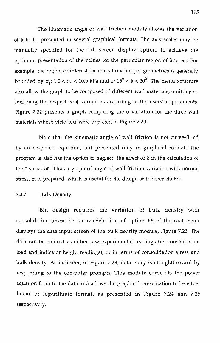
195

The kinematic angle of wall friction module allows the variation

of (|) to be presented in several graphical formats. The axis scales may be

manually specified for the full screen display option, to achieve the

optimum presentation of the values for the particular region of interest. For

example, the region of interest for mass flow hopper geometries is generally

bounded by Gy 1.0 < o^ < 10.0 kPa and ^•, 15° < <]) < 30°. The menu structure

also allow the graph to be composed of different wall materials, omitting or

including the respective (j) variations according to the users' requirements.

Figure 7.22 presents a graph comparing the ^ variation for the three wall

materials whose yield loci were depicted in Figure 7.20.

Note that the kinematic angle of wall friction is not curve-fitted

by an empirical equation, but presented only in graphical format. The

program is also has the option to neglect the effect of 8 in the calculation of

the ^ variation. Thus a graph of angle of wall friction variation with normal

stress, o, is prepared, which is useful for the design of transfer chutes.

7.3.7 Bulk Density

Bin design requires the variation of bulk density with

consolidation stress be known.Selection of option F5 of the root menu

displays the data input screen of the bulk density module. Figure 7.23. The

data can be entered as either raw experimental readings (ie. consolidation

load and indicator height readings), or in terms of consolidation stress and

bulk density. As indicated in Figure 7.23, data entry is straightforward by

responding to the computer prompts. This module curve-fits the power

equation form to the data and allows the graphical presentation to be either

linear of logarithmic format, as presented in Figure 7.24 and 7.25

respectively.

196

40. - • — r r - ' — I — ' — I — ' — r - 1 — I — 1 — I — I — I — I — r - I — I — 1 — I — 1 — r

RUSTY MILD STEEL - LIN. -1-PRCTENE - LIN. -2-

304-2B STRINLESS STEEL - LIN. -3-

— 1 30.

20.

10.

n—I—I—•—r

I • 1 L_J 1_ J : l_ I I I _i 1 1 L

0. 10. 15. 20. MRJGR CONSOLIDRTIGN STRESS - kPa

KINEMATIC ANGLE OF NALL FRICTION MRTERIRL: RUN OF MINE CGRL TESTED: JSNURRY.1988 MOISTURE CONTENT: 107. Nom- TEMPERRTURE: RMBIENT

Figure 7.22: Typical Variation of (^ for Several Wall

Materials.

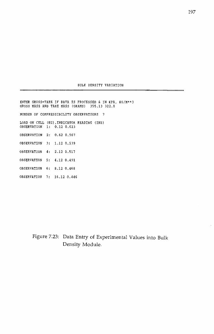
197

BULK DENSITY VARIATION

ENTER GROSS=TARE IF DATA IS PROCESSED & IN KPA, KG/M**3 GROSS MASS AND TARE MASS (GRAMS) 355.13 322.8

NUMBER OF COMPRESSIBILITY OBSERVATIONS 7

LOAD ON CELL (KG),INDICATOR READING (INS) OBSERVATION 1: 0.12 0.623

OBSERVATION 2: 0.62 0.567






Figure 7.23: Data Entry of Experimental Values into Bulk Density Module.

198

CO E

a>

I

tn UJ Q

1 0 0 0 . I I I I I I I I I I I '

900.

800. -

~i—1—I—r—I—r—T—T—r-

^. 700. 3 CD

600.

X

0.

I ' ' ' ' I -r-l—r—I—r-1—r ' "T •| I I I I I I I I I I I

OQ = 5 . 9 2 5 kPa PO = 7 7 5 . 0 1 Kg/mS

b = .0694 .Jl I — I — I l _ L I . . . . I t . . . . * . . . . I . . . . I ' . . . . I I • I • t I

25. 50. MRJOR CONSOLIDRTIGN STRESS - kPa

75.

BULK DENSITY MRTERIRL: RUN OF MINE CGRL MOISTURE CONTENT: 107 Nom.

Figure 7.24: Typical Bulk Density Variation

TESTED: JRNURRT,1988 TEMPERRTURE: RMBIENT

m ts

E

o>

100. c

I

tn 2 UJ Q

i :

OD

10.

0.. 1

1 1 1 1—I I I I

-X-

J I I I I I I I

T 1 1 1—I I I I

BULK DENSITY ¥r

A I I I t I I I

-1 1 1 1 — I I I I-I

-¥r -¥r

J I t I I I I 1

100. 1. 10. MRJOR CDNSGLIDRTION STRESS - kPa

BULK DENSITY MRTERIRL: RUN OF MINE CORL TESTED: JflNURRT,1988 MOISTURE CONTENT: 107 Nom. TEMPERRTURE: RMBIENT

Figure 7.25: Typical Bulk Density Variation, Logarithmic

Format.

199

7.3.8 Termination of a FP Computing Session

Selection of ESC from the root menu terminates the program

operation and a summary of the computing session is displayed on the text

monitor. This page provides information regarding the names and sizes of

the graphical and text data files. The report summary compiled from

processing the ROM coal example is presented in Appendix 1.3

7.4 DETERMINATION OF MASS FLOW HOPPER GEOMETRY

PARAMETERS; PROGRAM BD

The second computer program, BD, determines the hopper

geometry design parameters for mass flow hoppers based on the empirical

equations representing the flow properties of the particular bulk solid (refer

to Table 7.1). The interactive operation of this program allows the user

complete flexibility in deciding the tasks of a computing session. For

example, entering (or editing) the relevant flow property equations and

then determining the geometry parameters for instantaneous or time

storage conditions with the proposed wall lining materials. Figure 7.26

presents the overall flow chart of BD and highlights this feature.

The BD consists of 2,218 lines of FORTRAN code arranged in 24

symbolic files (excluding the PLOT PACKAGE and IMSL routines).

Appendix J.l presents a summary of the size (bytes) and number of lines of

code for each file. The size of the executable file BD.EXE is 240 kilobytes. The

code listing of BDMAIN.FOR, the main calling program controlling the root

menu of the program is provided in Appendix J.2.

A major consideration of the program development is the

calculation of the flow factor, which is required to utilise the flow-no flow

concept depicted in Figure 1.2. The computer procedures must be

mathematically robust to successfully operate with the various

GHD

200

F2

Fl

C Enter Data Filenames D Enter Flow Property Equations, of, - Instantaneous and Time Flow Functions - Effective Angle of Internal Friction Variation - Bulk Density Variation - Wall Yield Loci of up to 10 Materials

Root Menu of Program, Select Option:

ESC - Finish Fl - Determine Mass Flow Hopper Geometry Parameters F2 - Alter Flow Property Equations

Main Menu of Mass Flow Hopper Geometry Determination Module. For the Particular Case Select:

i) Axisymmetric or Plane Flow Hopper Shape ii) Instantaneous or Time Flow Function iii) Wall Material

c Determine the Critical Flow Factor and <x.

Determine the Critical Outlet Dimension, B given ff, a, and <^.

C Calculate the Variation of pt, with Outlet Diemnsion and Display Plot.

D

D }

Figure 7.26: Flowchart of the Program BD.

201

combinations of flow function, wall yield loci and effective angle of internal

friction possible.

Figure 7.27 presents the general classifications of bulk solids, namely, free

flowing, simple and cohesive according to the respective flow functions.

Referring to Figure 7.27, critical arching dimensions and hopper wall slopes

can only be determined on the basis of cohesive arching for those flow

functions (FF-C) that intersect with relevant flow factor, while the geometry

parameters for a simple bulk solid (FF-B) are determined on the basis of wall

friction. No mass flow hopper geometry can be determined for the bulk

solid indicated by the flow function FF-D as it lies above the flow factor and

no intersection can occur. For this situation other forms of storage using

non-gravity reclaim methods must be employed.

For the program as first developed, Dwight [621 developed an

iterative procedure which converges to the critical value of a^ and ff. This

approach is necessary because the flow properties are expressed as a function

of Gy and changes in ff lead to new values of G^ (on intersection with the

flow function) and thus new values of ^ and 5. The empirical equations

developed by Arnold et al. [41 (Equations 4.2 and 4.3), which express hopper

wall slope as a function of 5 and ^, are referenced to provide an a value (on

the mass flow boundary. Figure 1.3). Then, knowing the values of a, ^ and

5, the flow factor can then be calculated by solving the total differential

equations representing the Jenike radial stress field [1] simultaneously

under certain boundary conditions. A differential equation solver [64] using

a fifth order Runge-Kutta approximation is employed in the solution of

these equations.

The updated values of ^ and 6 then allow a new estimate of the

flow factor to be found, and the procedure is repeated until the difference

between successive flow factor values are within an acceptable tolerance

202

(FF - D)

Flow Factor

Cohesive Bulk Solid (FF - C)

Simple Bulk Solid (FF - B)

Free Flowing Bulk Solid (FF - A)

Major Consolidation Stress

Figure 7.27: Bulk Solid Classifications.

203

(nominally 0.001). A problem with this approach is the excessive

computation time involved when either of the following cases occur.

• a mass flow hopper design is not possible for the set of relevant

flow properties, eg. the flow function FF-D, Figure 7.27, positioned

above the possible range of flow factors.

• a critical mass flow geometry cannot be determined because of

high values of wall friction. This typically occurs for bulk solids

that have only low to moderately strong flow functions, and a

wall yield locus displaying a strong adhesion. As a result,

intersections between initial flow factor values and flow function

yield values of a^ for which ^ cannot be calculated. This

calculation is indeterminate because Oj is below the limiting

value of o^ which defines a Mohr circle of stress that is tangent to

the wall yield locus. Thus the Mohr circles generated for smaller

o^ values do not contact the wall yield locus. Figure F.18 for

-0.5mm Westcliff Product coal at 15% moisture illustrates this

concept. Here, a value of (]) cannot be calculated for o^ < 3.0 kPa. In

this situation, the geometry for mass flow is based on wall friction

considerations, (the same as for a simple bulk solid), rather than

cohesive arching.

The two aspects discussed above have been eliminated, and the

complete critical geometry determination substantially simplified by

incorporating the graphical design nomogram procedures developed by

Moore and Arnold [48, 67] and discussed in Chapter 5. This is achieved since

the complete state of the flow factor variation (unique to the particular set

of {[), 5 and m), is represented by the flow factor locus, (refer to Figure 7.28).

204

12 r

tfi 1 0 «}

CD •

l-H

01

o u

F/oiy Factor Locus

2 4 6 8 10

Major Consolidation Stress

12

Figure 7.28: Computer Application of the Flow Factor Locus Concept for the Determination of the Critical Hopper Geometry.

205

The computer program follows the operation of the graphical

nomogram method, where the intersection between the flow function and

the flow factor locus defines the critical design point and the value of Gy

This procedure is detailed in Figure 7.28, where for flow function FF-C,

point B represents the critical design point.

Representing the flow factor locus by a three parameter equation

(with a defined lower endpoint. A), it is computationally straightforward to

determine the critical design point by the intersection with the relevant

flow function. The endpoint A, represents the lower limit of G^ for which a

flow factor can be determined. Further substantial benefits of this approach

are realised, when considering the two aspects previously discussed.

Referring to Figure 7.28, the flow function positions, such as FF-D, which

cannot yield a mass flow hopper geometry can be now easily recognised

mathematically (rather than using an iterative procedure).

In relation to the second aspect. Figure 7.28 displays the flow

function, FF-B, positioned below the flow factor locus endpoint A,

indicating that a critical geometry cannot be determined based on cohesive

arching. This flow function is then similar in nature to the simple bulk

solid represented by FF-A, with no critical geometry applicable and the

variation of a and B is determined by incrementing o^ for values greater

than endpoint A.

The other design data presentation determined is the variation of

a with span B. As introduced in previous sections, (j) may not be constant

but vary with Gy with ^ having high values at low a^ values. This trend is

then utilised by allowing larger hopper wall slopes for hopper outlet

dimensions above the critical. The increase of consolidation stress with the

increased span in turn leads to a reduced (]) value and hence an increased

hopper wall slope angle. A typical a versus B graph is depicted in Figure 1.8.

206

This graph indicates how a tends to a limiting value of a as the rate of

change of ^ decreases in the higher stress range of o^. The program BD

calculates this variation by incrementing a^ from the critical value to an

upper limit of o^ = 20 kPa) and determining the respective values of a and

B.

The operation of BD will now be described by referring to figures

presenting the various text screen and graphics displays. The empirical

equations representing the flow properties determined by FP for the ROM

coal example will used to determine the hopper geometry parameters.

7.4.1 Execution of Program BD

The program execution is started by entering \BD\BD and the

titiepage. Figure 7.29, is displayed after the program has been loaded into

memory. After the titiepage, the data output filenames are entered, in a

similar fashion to the initial stages of FP. The two data output files for BD

store a summary of all flow property equations used in the analysis, and the

second file stores the graphical displays selected by the operator as plot files.

The next stage involves the input of the bulk solid name and the

relevant flow property empirical equations. This information can be

entered from the keyboard, or by data file. If the keyboard approach is

selected, the operator is requested for a data file name, to store the entered

equations for subsequent computing sessions.

Figures 7.30 to 7.36 present the displays of the text monitor for the

input of the bulk material name and flow properties. As indicated in these

figures, utilising formatted text screens allows the characteristic equation to

be displayed and the cursor positioned within each cell for the entry of the

coefficients. This technique is a convenient and rapid means of data entry

MASS FLOW HOPPER GEOMETRY DETERMIATION

DEPARTMENT OF MECHANICAL ENGINEERING

UNIVERSITY OF WOLLONGONG

Developed by: B.A.MOORE N.B.MASON

VERSION 2.0

January, 1988

Press H for help or any key to continue

Figure 7.29: Titiepage of Program BD.

BULK SOLID FLOW CHARACTERISTICS

DATA ENTRY METHOD Fl - KEYBOARD F2 - DATA FILE

OPTION

DATA INPUT FILE <BD-INPUT.DAT>: ROM-INPUT.DAT (FOR SUBSEQUENT RERUNS)

ENTER THE MATERIAL NAME: RUN OF MINE COAL, 10% Nora.

207

Figure 7.30: Flow Property Data Input for BD: Bulk SoHd Name.


208

FLOW FUNCTION DATA ENTRY

ESC - NOT AVALIABLE Fl - INSTANTANEOUS FLOW FUNCTION

OPTION -

SIGMAC = (0.41 )*SIGMA1+(1.46 ) KPa

Figure 7.31: Flow Property Data Input for BD: Instantaneous Flow Function.


FLOW FUNCTION DATA ENTRY

ESC - NOT AVALIABLE Fl - TIME FLOW FUNCTION

OPTION

SIGMAC = (0.43 )*SIGMA1+(1.96 ) KPa

Figure 7.32: Flow Property Data Input for BD: Time Flow Function.

209


EFFECTIVE ANGLE OF INTERNAL FRICTION:

Fl - CONSTANT VALUE F2 - TWO PARAMETER EQUATION F3 - THREE PARAMETER EQUATION

OPTION -

DELTA = (1.52 )- (-3358.91) DEGREES (SIGMA1+(52.71 ))

Figure 7.33: Flow Property Data Input for BD: Effective Angle of Internal Friction.


EQUATION FOR BULK DENSITY VARIATION

T**(0.0694 ) BULK DENSITY = (775.01 )* SIGMAl

<5.925> Kg/M**3

Figure 7.34: Flow Property Data Input for BD: Bulk Density Variation.

210

HOPPER GEOMETRY DESIGN

WALL YIELD LOCI DATA ENTRY ESC - RETURN TO MAIN MENU Fl - ENTER WALL MATERIAL NAME

OPTION -

WALL MATERIAL NAME FOR W.Y.L. No. 1 :RUSTY MS

WALL YIELD LOCI EQUATION: Fl - CONSTANT PHI

F2 - TWO PARAMETER EQUATION F3 - THREE PARAMETER EQUATION

OPTION

TAU = (41,00 )- (2344.19) KPa. (SIGMA1+(57.21 )

Figure 7.35: Flow Property Data Input for BD: Wall Yield

Locus, Three Parameter Equation.


WALL YIELD LOCI DATA ENTRY ESC - RETURN TO MAIN MENU Fl - ENTER WALL MATERIAL NAME

OPTION -

WALL MATERIAL NAME FOR W.Y.L. No. 3 :3G4-2B STAINLESS STEEL

WALL YIELD LOCI EQUATION: Fl - CONSTANT PHI F2 - TWO PARAMETER EQUATION F3 - THREE PARAMETER EQUATION

OPTION -

TAU = (0.28 )*SIGMA1 + (0.35 ) KPa

Figure 7.36: Flow Property Data Input for BD: Wall Yield Locus, Linear Equation.

211

HOPPER GEOMETRY DESIGN

SELECT FROM THE FOLLOWING

ESC - FINISH Fl - CALCULATE MASS FLOW HOPPER GEOMETRY F2 - ALTER BULK SOLID FLOW PROPERTIES

OPTION -

Figure 7.37: Root Menu of Program BD.

212

and minimises typing mistakes. The program can process up to ten wall

materials.

On completion of the data entry of the flow properties, the root menu of

BD, Figure 7.37 is displayed. The structure of BD has been arranged to allow

additional aspects of bin design to be incorporated as modules in the root

menu in the future. Such aspects include funnel flow geometry design,

feeder load calculations, bin wall loadings and bin volume/dimension

design graphs.

7.4.2 Determination of Mass Flow Hopper Geometry Parameters

On selection of option Fl, from the root menu, the text monitor

displays Figure 7.38. This is the main menu page for the mass flow

geometry determination module and allows the hopper shape and relevant

flow properties to be nominated. As indicated, this screen arrangement

provides a complete and clearly formatted schedule for each calculation.

After selection of the wall lining material, the program calculates

the critical mass flow parameters and displays the results on the text

monitor as presented in Figure 7.39. Note the values of a and B have been

rounded off in the display, with a to the nearest 0.5° above and B to the

nearest multiple of 5mm. Selection of option F3 if more detailed

information is required, displays the parameter values at the critical design

point involved in the geometry calculation. Figure 7.40.

To generate of the a versus B graph, options Fl or F2 are selected

from the screen format displayed in Figure 7.39. The first option calculates

the relevant values and stores them for subsequent plotting with other

graphs for different wall materials or hopper shapes. The second option

calculates the variation and displays the plot on the graphics monitor.

213

MASS FLOW HOPPER - CRITICAL GEOMETRY PARAMETERS

BIN GEOMETRY Fl - AXISYMMETRIC F2 - PLANE FLOW

OPTION - < Fl >

FLOW FUNCTION Fl - INSTANTANEOUS F2 - TIME

WALL MATERIALS

WALL MATERIAL RUSTY MS PACTENE 304-2B SS

OPTION —

1 2 3

C Fl >

No.

ENTER WALL MATERIAL No. < 1 >


Module.

214


CRITICAL DIMENSION FOR BIN HOPPER GEOMETRY

HOPPER HALF ANGLE OUTLET WIDTH

30.5 Degrees 425. mm

INSTANTANEOUS FLOW FUNCTION PLANE FLOW HOPPER GEOMETRY

WALL MATERIAL: 304-2B SS

ESC - RETURN TO MAIN MENU Fl - DETERMINE ALPHA VS B VARIATION F2 - DETERMINE AND PLOT ALPHA VS B VARIATION F3 - DISPLAY PARAMETERS AT CRITICAL DESIGN POINT

OPTION

Figure 7.39: Text Screen Displaying the Critical Mass Flow Hopper Geometry Parameters.


CRITICAL DIMENSION FOR BIN HOPPER GEOMETRY

HOPPER HALF ANGLE OUTLET WIDTH

30.5 Degrees 425. mm

INSTANTANEOUS FLOW FUNCTION PLANE FLOW HOPPER GEOMETRY

WALL MATERIAL: 304-2B SS

PARAMETERS AT THE CRITICAL DESIGN POINT

MAJOR CONSOLIDATION STRESS: 2.911 kPa CRITICAL FLOW FACTOR: 1.097

KINEMATIC ANGLE OF WALL FRICTION: 22.95 Deg. EFFECTIVE ANGLE OF INT. FRICTION: 61,91 Deg,

ESC - RETURN TO PREVIOUS MENU

Figure 7.40: Text Screen Displaying tiie Critical Mass Flow Hopper Geometry Parameters and Flow Property Values at the Critical Design Point.

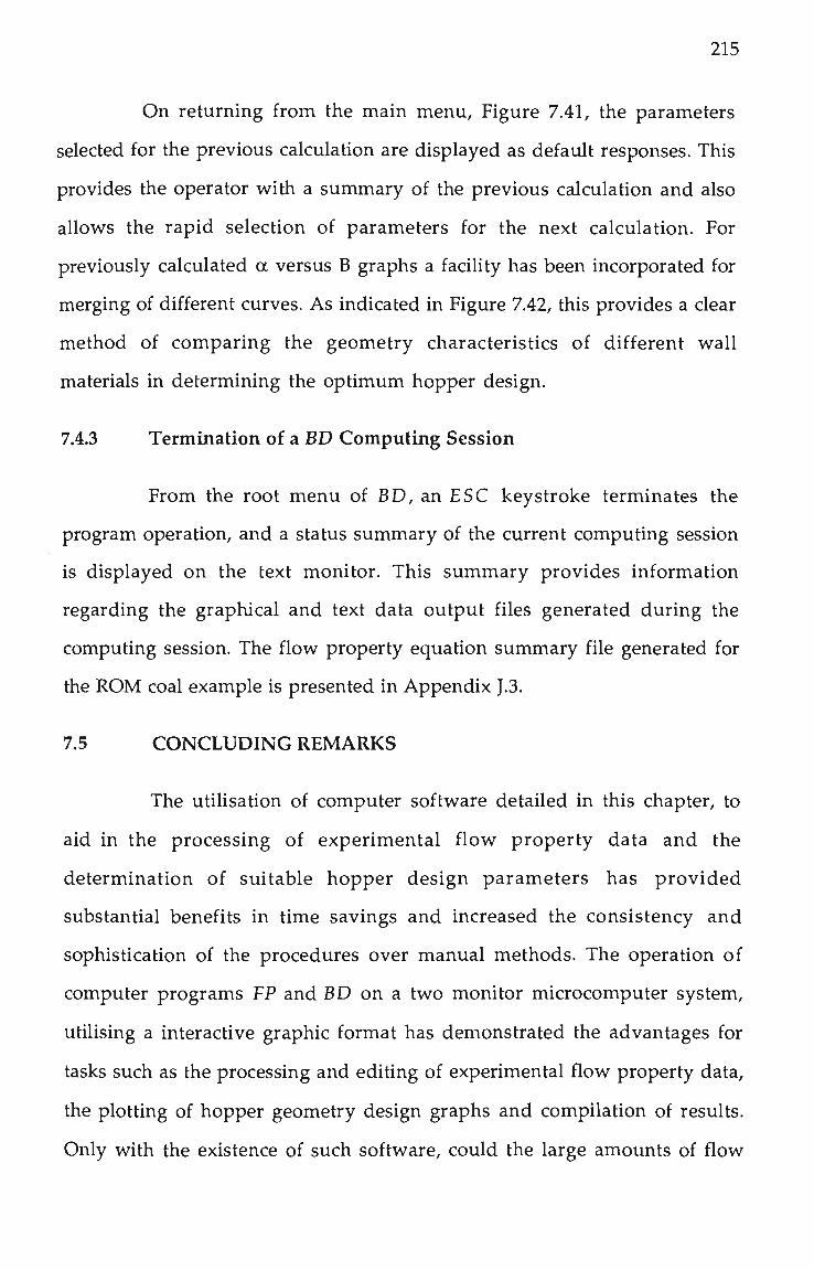
215

On returning from the main menu. Figure 7.41, the parameters

selected for the previous calculation are displayed as default responses. This

provides the operator with a summary of the previous calculation and also

allows the rapid selection of parameters for the next calculation. For

previously calculated a versus B graphs a facility has been incorporated for

merging of different curves. As indicated in Figure 7.42, this provides a clear

method of comparing the geometry characteristics of different wall

materials in determining the optimum hopper design.

7.4.3 Termination of a BD Computing Session

From the root menu of BD, an ESC keystroke terminates the

program operation, and a status summary of the current computing session

is displayed on the text monitor. This summary provides information

regarding the graphical and text data output files generated during the

computing session. The flow property equation summary file generated for

the ROM coal example is presented in Appendix J.3.


The utilisation of computer software detailed in this chapter, to

aid in the processing of experimental flow property data and the

determination of suitable hopper design parameters has provided

substantial benefits in time savings and increased the consistency and

sophistication of the procedures over manual methods. The operation of

computer programs FP and BD on a two monitor microcomputer system,

utilising a interactive graphic format has demonstrated the advantages for

tasks such as the processing and editing of experimental flow property data,

the plotting of hopper geometry design graphs and compilation of results.

Only with the existence of such software, could the large amounts of flow

216


BIN GEOMETRY

FLOW FUNCTION

WALL MATERIALS

WALL MATERIAL RUSTY MS PACTENE 304-2B SS

Fl - AXISYMMETRIC F2 - PLANE FLOW

OPTION - < F2 >

Fl - INSTANTANEOUS F2 - TIME

OPTION - < Fl >

No. 1 2 3

ENTER WALL MATERIAL No. < 3 >


Module Highlighting the Default Responses

from the Previous Geometry Calculation,

217

• « >-LU

— to +> cn c

2 : QD IS) CM

— 1 II — r^

10 C55

— -(-> fO UJ

z: 2: S I LU

— 1— II — CJ

0 cr

— +> CO 10 z :

z : (S > -

— 1— II — CD

(0 ZD ic: - - < z : 2 oo cx j s r s : Q_ c n 2 : 3 az t n

L' I ' I ' 111 • I ' " I ' I ' 111' I ' I ' I ' 111' I ' I ' I ' I ' I ' I ' I ' 111' I ' I ' I ' I ' I ' I ' I ' I ' I ' I ' I • J CO

s

m

cn u

C_) •

cn

<~-v

cn ID l j j

•OC CMH-

LU

UJ 5 ®

= z °-( - " ^ Q.

n: ' ^ -•— . "

_ j " OC F F -U J Q c

is)OQ

•LU

(S)UJ

CD o

LU cn CJ

CD

u_

UJ

ID

s l l 1 1 1 1 1 1 1 1 1 1 1 1 l l 11 l l I r 1 1 1 1 1 1 1 1 1 1 1 1 1 1 1 1 1 1 1 1 1 1 1 1 1 1 l l 1 1 1 1 1 1 1 1 1 1 1 1 1 1 1 1 1 1 1 1 1

S) ts) IS s ) IS) s SI i s a

ID • *

ca • ^

Ln on

s CO

iLn CM

(S C\J

LD (S

0 ^ 0

cn = ; L I _

-i .. <= a a

az o CD <si

JL —J •*

u_ o

o _J 0-

(S33yG3a) -UHdlB - y3ddOH 30 310NH 31blH

Figure 7.42: Graphical Presentation of the Variation of a

versus B for Several Wall Materials from the

Design Example.

218

property data and hopper geometry parameters presented in Appendices B

through G be processed and analysed.

Representing the flow properties by characteristic empirical equations,

namely, linear, three parameter and power equations, has proved a

convenient and accurate method of specifying the flow properties for input

into materials handling design programs. The three parameter equation

used to describe some of the flow properties has proved to be most versatile.

The determination of the mass flow hopper geometry parameters

by a computer program incorporating the flow factor locus approach [48]

(utilised in the graphical nomograms detailed in Chapter 5) has provided a

computer algorithm which is more direct and simpler than the previous

algorithm which used iterative procedures. Since the flow factor locus

describes the complete variation of the flow factor with o^ (unique to the the

particular set of 5, <t) and m values), the calculation of hopper geometry

parameters can be determined directly by comparing the flow factor locus

with flow functions of the bulk solid.

219

CHAPTER 8

CONCLUSIONS

The design of storage facilities to ensure reliable and predictable

performance should be approached as a four step procedure:

• Determination of the strength and other flow properties of the

bulk solid for the worst representative conditions likely to occur

in practice.

• Determination of the bin geometry to give the desired capacity

and to achieve the required flow pattern with acceptable flow

characteristics and to ensure that discharge is reliable and

predictable.

• Estimation of the loads exerted on the bin walls and feeder under

operating conditions.

• Design and detailing of the bin structure and hopper feeder

interface.

This work has studied the two initial phases of the above

procedure, specifically related to the design of mass flow bins for the storage

of black coal. This has involved an investigation of the influence of physical

variables of coal samples on the respective flow properties and the design

procedures for determination of the mass flow hopper geometry

parameters.

8.1 FLOW PROPERTIES OF BLACK COAL

A rigorous flow property testing program was conducted on coal

samples from the Southern Coalfields (Illawarra Measures) of the Sydney

Basin. This coal is a hard black coal type varying in rank from sub-

bituminous to semi-anthracite.

220

A standardised testing procedure was developed for the Jenike-

type Direct Shear Tester. This procedure minimised operator and data

interpretation related errors in the shear testing of the coal samples for the

flow property testing program. Important aspects of this procedure include

the need to consider the yield loci of different consolidation levels as a

family of related curves, the yield loci should be parallel or fan out slightly,

and that the end points of the yield loci lie on a line passing through or just

above the origin. The prorating procedure of Jenike [68] for reducing the

scatter of yield loci data coordinates was found to work well.

The testing program identified the physical variables of free

moisture content, particle top size and distribution, and time of storage at

rest to be the most significant influence on the flow properties. Other factors

such as particle shape, coal rank, and ash content (<15%), were shown to be

minor considerations.

The following observations regarding the flow properties of coal

are relevant:

• Coal displays significant strength even under instantaneous

conditions. This strength increases dramatically with time of

storage at rest, particularly at higher moisture contents.

• The strength of coal, as indicated by the flow function, displays

maximal strength for moisture contents in the range of 10 - 15%.

These moisture content levels represent the typical range of most

handling operations, and are significantly less than the saturation

moisture content.

• The instantaneous and time flow function have geometrically

similar gradients at low consolidation stresses.

• The effective angle of internal friction displays a decreasing

variation with increasing consolidation stress for moist coal. The

221

average value of 5 increases with increasing moisture content,

typically 45° for air dried and 50 - 55° at 6% levels, to 60°-70° for

10% and 15% moisture contents.

• Significant variations were displayed in the wall friction

coefficients for different wall lining materials. At low

consolidation stresses, moist coal displays a rapid decrease in the

kinematic angle of wall friction with increasing o^. This feature is

attributable to adhesion of the moist coal to some surfaces, for

example 304-2B stainless steel. Variable angles of wall friction

were also displayed for those materials that have convex upward

wall yield loci.

• The maximum bulk density values were determined for air dried

and 15% moisture content samples. For intermediate moisture

levels bulk density values decreased from those determined for

the air dried level. The bulk density variation increases 3 3

asymptotically to limiting values of 1000 kg/m and 1075kg/m for 10% and 15% moisture contents respectively.

Flow property tests were conducted on samples prepared at

-1.00mm, -2.36mm and -4.00mm. Comparison of the -2.36mm and -4.00mm

sample results are similar for the various flow properties, and does not

indicate any less conservative results for the -4.00mm samples. The

-1.00mm test sample results displayed significantly greater stronger flow

functions with more scatter compared to the other two samples. The

combined action of fine particle distribution and high moisture content

substantially reduces the handleability of coal. Shear tests on -1.00mm at

10% and 15% moisture contents indicate a values of up to twice the values

determined for the two larger particle cut test samples.

The flow properties of coal samples mixed with Kaolin and

Bentonite clays (to simulate high ash content coals) were determined and

222

display similar results to those of high fines content coals. The major

feature of the clay sample flow properties was the extremely strong time

flow functions, which often displayed a cementing action. In addition to

displaying the adverse flow properties for high clay content coals, these

results also highlight the effect of a high fines content in reducing the coal

handleability. This situation can occur for soft friable coals which degrade

easily during handling operations. The higher fines content then leads to

higher moisture retention capabilities and a consequent deterioration of the

handleability characteristics,

8.2 DESIGN PROCEDURES FOR THE DETERMINATION OF MASS

FLOW HOPPER GEOMETRY PARAMETERS

Manual and computer aided design approaches for the

determination of mass flow hopper geometry parameters were considered

in this work.

Chapter 4 presents the development of an alternative

presentation of the original Jenike flow factor charts, for the display of the

design parameters for mass flow hoppers. These alternative charts present

only the critical design values of flow factor and a in the border region

between mass flow and funnel flow for axisymmetric and plane flow

hoppers.

The charts eliminate the need for imprecise parameter

interpolations (necessary with Jenike flow factor charts) by displaying the

required design parameters of ff and a as a function of the effective angle of

internal friction and kinematic angle of wall friction. This format also

provides an overall assessment of the variation of ff and a along the mass

flow design limits, and the sensitivity of these two parameters with 6 and (t)

values .

223

The alternative presentation of the hopper design parameters has

been utilised in the development of graphical nomograms or worksheets

for the manual determination of a and B. Utilising this presentation of

hopper design data, where all parameters are displayed as a function of a

common independent variable, Gy the following aspects are clearly detailed:

• the relation between hopper outlet dimension and Gy

• the correlation of ([) with the respective values of wall slope.

• the sensitivity of the flow function position on values of B. This

is important for low values of the critical design point, where G.

may be remote from the experimental data points used to

determine the flow function.

The critical hopper geometry design point is determined by the

intersection between the flow factor locus and the respective flow function.

An important feature of the flow factor locus is the lower end point, which

specifies the lower limit of o^ for which a ff and hence a critical hopper

geometry can be determined. The lower limit is determined for a particular

hopper shape, on the basis of ^ and 8, has typical values of Gy 2.5 < o^ < 3.5

kPa for coals at 10% and 15% moisture content with 304-2B stainless steel.

The usefulness of the graphical nomogram is further

demonstrated when the values of a and B are required to satisfy additional

design constraints. Typical constraints involved in the detailing of the

hopper geometry includes allowable headroom, maximim lump size, feeder

arrangements and proposed discharge flow rates. These constraints can be

added to the nomogram to highlight those regions which satisfy the design

objectives.

The nomogram presentation also highlights the significant

influence of ((), and the minor effect of 5 in generating the a versus a^ and B

versus a^ design curves. These features can be utilised by the designer for

224

hoppers where the value of B is known to be greater than the critical (based

on experience or previous hopper designs). For this situation the flow

function need not be known and the hopper design can be based on the wall

friction and compressibility tests only. This advantage of this approach is

that both of these laboratory tests are quite straightforward and fast, without

the need for shear testing using the sophisticated equipment and procedures

involved with the Jenike-type Direct Shear Tester.

Chapter 6 presents the development of standardised hopper

design guidelines, based on the results of the flow property testing program

and the Jenike hopper design procedures. The guidelines apply to hard black

coals, similar to those tested, namely, a rank of sub-bituminous to

semi-anthracite, an ash content less than 15%, HGI < 60, and 304-2B

stainless steel as the hopper wall lining material.

Two approaches are presented. The first, specifies the expected

values of a and B (under instantaneous and time storage conditions) by

analysing statistically the hopper geometry parameter results presented in

Appendix H, by the Students' t Distribution. The expected values are then

expressed as the mean value within a 90% confidence interval.

For example, the expected geometry parameter ranges for 10%

moisture content coal are a„: 20.5° < a^ < 22.5°, a„ : 30.0 < a „ < 32.0°, c c ' p P

B^ :950 < B < 1170mm and B : 435 < B < 535mm. This information is c c P P

useful for providing values required for preliminary engineering layouts or

for reviewing existing coal bins that are experiencing storage problems.

The second approach considers the mean and range of the various

flow property values, and the respective range of flow factors relevant to the

determination of the critical hopper design. This analysis allows values of a

and B to be estimated from a reduced flow property testing program. Tests

are required only to determine or confirm these property values which

225

exert significant influence on a and B, while for those properties that have a

minor effect, (such as 5), expected values displayed on graphs for various

moisture contents can be used.

To provide an estimate oi Gy for the calculation of the outlet

dimension B, this second approach requires the determination of one yield

locus, to provide a reference point for the flow function. The value of Oj at

the critical design point can be estimated by projecting the flow function

(passing through (Gy GJ with a slope parallel to the graphically presented

mean flow function) and intersecting with the mean flow factor range.

Selection of the consolidation level of the shear test is required to

ensure the coordinate (Gy GJ determined lies within the o^ range specified

for each moisture content. Errors in estimation of G^ can occur if this

coordinate is far outside these ranges.

The procedure emphasises the need to know the kinematic angle

of wall friction variation for proposed materials and the bulk density

variation for mass flow hopper design. This approach extends on the last

aspect discussed regarding the graphical nomogram, by providing expected

flow property and flow factor trends close to the critical design point for

hopper designs.

Chapter 7 provides details of two computer programs, FP and BD,

which process and analyse experimental flow property data, and determine

the mass flow hopper geometry parameters respectively. Utilisation of these

programs have demonstrated substantial benefits in time savings and

increased consistency and sophistication of the procedures over manual

methods. Both programs have been developed to operate on a two monitor

microcomputer system utilising an iterative graphical format.

226

The program FP, processes the experimental flow properties and

presents them graphically and by characteristic empirical equations. These

equations have proved a convenient and accurate method of specifying the

flow properties for input into other matrials handling computer programs.

The three parameter equation used to describe some of the flow properties

has proved to be most versatiole.

Program BD determines the critical mass flow hopper geometry

based on the empirical equations specifying the various flow properties. In

addition to determining the critical values of a and B, the program

calculates the variation of a with B for values greater than the critical. This

design graph has proved useful for the design of hoppers where the

proposed wall lining material has a variable kinematic angle of wall friction

and increased values of a utilised for increased values of B.

For determination of the critical design point, the program

incorporates the flow factor locus approach (utilised in the graphical

nomograms). This allows a direct and straightforward computer algorithm

to be implemented, where the existence of, and values of hopper wall slope

and outlet span can be found by comparing the relevant flow function with

the flow factor locus.

8.3 FUTURE RESEARCH DIRECTIONS

Several topics requiring further research have been identified

during the course of this work. The coal flow property testing program

highlighted the following aspects:

• Investigation of the relation between the surface moisture

content for the complete coal distribution and the -4.00mm (or -

2.36mm) coal sample used for flow property testing. Clarification

of the proportion of surface moisture existing with the fines

227

portion (0 x -4.00mm) of the complete coal would allow the

preparation of test samples at the actual level.

Preparation of the sample at the correct moisture content would

then reduce the degree of conservatism introduced into the flow

property test results, particularly for the flow function.

As highlighted in this work, the shear testing is now guided by a

standardised procedure. The procedure utilises the prorating of

instantaneous yield loci points suggested by Jenike [68,69]. There is

a need to extend this standard procedure to incorporate the testing

of time yield loci. Generally it was found that greater scatter

occurs with the time yield loci data than with the instantaneous

points. A prorating procedure proposed by Jenike [68], was applied

to experimental data in preliminary tests, however little

reduction in the scatter of time yield loci data occurred.

Relevant to the hopper design procedures, accurate

determination of the time flow function is important, as this is

often the limiting property for the calculation of the critical outiet

dimension.

The second flow property test that requires standardisation is the

Coulomb friction test for determination of the wall friction

angles. Chapters 5 and 6 highlight the importance of this

parameter in mass flow hopper design. It is therefore important

that this procedure be standardised to provide increased

consistency in measuring the wall yield locus and an indication of

the (j) variation that can be expected.

228

Currently slightly different wall yield loci results can be obtained

by either increasing or decreasing the consolidation weights

during the test, or using different weight increments.

Chapter 6 has detailed the development of standardised hopper

design guidelines. The development should be continued to increase the

number of data values statistically analysed, and to incorporate hopper

geometry design parameters determined for other coals from different

coalfields (but which satisfy the stated terms of reference).

The guidelines should be extended to include data on other wall

lining materials. In recent times other wall lining materials such as 3CR12

and 301 stainless steel commonly have been specified for application in coal

storage facilities.

The further development of computer software for bin design,

specifically configured for microcomputers is a worthwhile direction. The

structure of the program BD has been arranged conveniently to incorporate

additional design modules. Suggested future modules include funnel flow

bin design, feeder load predictions, bin wall load predictions and bin

volume/overall dimension design graphs for the preliminary planning and

sizing of storage facilities.

Recent developments in computer software incorporating

artificial intelligence offer a longer term research goal for the application of

computer aided design techniques to the design of bulk solid storage

facilities. Interpretation of the flow properties and hopper geometry

parameter design data in designing a cost efficient installation that satisfies

various constraints requires significant expertise and experience.

Development of a knowledge based expert system combining the

expertise of a specialist with the relevant technical engineering data

229

(including hopper geometry parameters, bulk material characteristics,

standard feeder arrangements and site details) for the design and detailing

of storage bins would be an extremely useful facility.

230

REFERENCES

1. Jenike, A.W.

'Gravity Flow of Bulk SoUds', Bui. 108 Utah Engng. Exper. Station,

University of Utah, 1961.

2. Johanson, J.R.

•Stiress and Velocity Fields in Gravity Flow of Bulk Solids', Bui. 116

Utah Engng. Exper. Station, University of Utah, 1962.

3. Jenike, A.W.

'Storage and Flow of Solids', Bui. 123 Utah Engng. Exper.Station,

University of Utah, 1964.

4. Arnold, P.C, McLean, A.G. and Roberts, A.W.

'Bulk Solids: Storage, Flow and Handling', The University of

Newcastle Research Associates (TUNRA) Ltd., 2nd Edition, 1980.

5. Carson, J.W.

'Design of Bins and Feeders for Reliable Minerals Flow', Mining

Engineering, March, 1983, pp. 229 - 234.

6. Wolf, E.F., and van Hohenleiten, H.L.

'Experimental Study of the Flow of Coal in Chutes at Riverside

Generating Station', Trans. ASME, April, 1947, pp. 585 - 599.

7. Leggett, R.F.

'Clogging of Bituminous Coal in Bunkers', Trans. ASME, April, 1947,

pp. 525-531.

8. Hall, D.A., and Cutress, J.G.

'The Effect of Fines Content, Moisture and Added Oil on the Handling

of Small Coal', J. Inst. Fuel, Vol. 33,1960, pp. 63 - 72.

231

9. Mikka, R.A., and Smithan, J.B.

'Coal Handleability Assessment', Proc. Third Australian Coal

Preparation Conference, WoUongong, Nov., 1986, pp. 12 - 27.

10. Crisafuin, P., Le Page, A.J. and Stockton, N.D.

'The Effects of Clay Contamination on the Handling and Preparation

of Walloon Coals', Proc. Third Australian Coal Preparation

Conference, WoUongong, Nov., 1986, pp. 45 - 65.

11. Jones, G.S.

'An Investigation into Factors Affecting the Handlability of Industrial

Smalls', MRDE Report No 10,1970. National Coal Board, 21 pages.

12. Royal, T.A and Costello, R.F.

'Gravity Flow of Solids Databook: Measurement of Surface Moisture of

Coal'. US Department of Energy, Report DOE/NC/14101-1847,

September, 1984, 59 pages.

13. Foster - Miller Assoc.

'Increasing Mine Car Coal Bulk Density by Vibration', U.S. Department

of Energy, 1981, Final Report, DOE/ET/12498 - Tl, 227 pages.

14. Leung, L.S. and Osborne, J.L.

'Flow Properties and Flow Behaviour of Coal in Storage, Pneumatic

Conveying, Standpipe Flows and Fluidisation - Australian Coals',

NERDDP Report EG/43, Jan., 1982,168 pages.

15. Day, R. and Hedley, A.B.

'Modelling the Flow Characteristics of Moist Particulate Materials',

Proc. European Symposium on Particle Technology, 1980, Amsterdam,

NL,pp 1103-1112.

232

16. McEwen, P.P., Correto, W.P. and Reed, T.R.

'The Storage and Handling of Dewatered Pipeline Coal', Proc.

Industrial Powder and Bulk Solids Handling and Processing

Conference, Rosemont, 111, USA, 1983 pp 673 - 686.

17. Arnold, P.C, McLean, A.G. and Moore, B.A.

'Flow Properties of Coal for Storage Bin Design', NERDDP Report,

79/9079, March, 1985,243 pages.

18. Wood, P.A.

'Fundamentals of Bulk Solids Flow', Report No. ICTIS/TR31, lEA Coal

Research, London, Jan., 1986. 64 pages.

19. Bloyden, LD.

'Geology of Australian Coalfields - Some Other Coal Fields' in Cook

A.C (Ed.), Australian Black Coal - its Occurrence, Mining, Preparation

and Use. AIMM Conference 1975, Illawarra Branch, pp. 19 - 37.

20. Wilson, R.G.

'Illawarra Coal Measures: A Southern Coalfield', in Packham G.H.

(Ed.), Geology of New South Wales, J. Geol. Soc. Aust., 1969,16,

pp.370 - 379.

21. Anon. BHP Brochure

'BHP Coal for Steel', 1971. 15pp.

22. Robinson, J.B. and Shields, D.J.

'The Permian Coal Deposits of N.S.W.' in Cook, A.C. (Ed.), Australian

Black Coal - its Occurrence, Mining, Preparation and Use. AIMM

Conference 1975, Illawarra Branch, pp 87 -103.

23. 'Black Coal in Australia 1979 -1980 - A Statistical Year Book'

Joint Coal Board, Australia, March,1981, 229 pages.

233

24. AS 2096 - 1977

'Classification Systems for Australian Hard Coals', Standards

Association of AustraUa.

25. Facer, R.A., Cook, A.C. and Beck, A.E

'Thermal Property and Coal Rank in Rocks and Coal Seams of the

Southern Sydney Basin, N.S.W.; A Palaeogeothermal Exploration of

Coalification', Int. J. Coal Geology, Vol. 1, No. 1, pp. 1 -17.

26. Nicol, S.K., Day, J.C, Firth, B.A., Gallagher, E. and Swanson, A.R.,

'Current Trends in Fine Coal Treatment', BHP Tech. Bull. Vol. 23,

No.2, Nov., 1979, pp, 41 - 46.

27. BS 1976 :1952

'Methods for the Use of BS Fine Mesh Test Sieves', British Standards

Association.

28. Winegartner, E.C

'Rosin - Rammler Charts and Their Application to Size Distribution

Problems', Proc. 10th. Annual Seminar on Bulk Material Handling,

Univ. of Pittsburgh, 1980, pp. 23 - 46.

29. DR 86111

'Flow Properties of Coal', Draft Australian Standard For Comment,

Standards Association of Australia, June, 1986.

30. Ooms, M. and Roberts, A.W.

'Hopper Surface Finish and Friction Interrelation with Respect to Bulk

Solids Flow from Storage Bins', Proc. Int. Conference on Bulk

Materials Storage, Handling and Transportation, lEAust., Newcastie,

AustraUa, August, 1983, pp. 237 - 243.

234

31. ter Borg, L.

'Evaluation of Shear Test Results on Bulk Solids in the Chemical

Industry', German Chem. Engng, Vol. 5, Pt.l, 1982, pp. 59 - 63.

32. Dau, G.

'Measurement of the Wall Friction Angle for Bulk Solids on Different

Wall Materials.', Aufbereitungs-Technik Vol.24, Pt.ll , 1983,

pp. 633 - 646.

33. Rappen, A. and Wright, H.

'The Use of Air Cannons to Solve Coal Flow Problems in Bunkers',

Aufbereitiings-Technik, Vol.25, Pt.4,1984, pp. 200 - 208.

34. Fang, S.J., Duffy, T.J., Kao, G.C and Fujii, R.K.

'Coal Flow Problems and Solutions for Power Plant Silos.', Proc. 9th.

Annual Powder and Bulk Solids Conference, 1984, Rosemont, 111. USA

pp 591-601.

35. Bennett, A.L.

'Coal Flow and Design Considerations, Bunker to Pulveriser.', Stock

Equipment Co., U.S.A. 1979, 32 pages.

36. Schwedes, J.

'The Influence of Wall Friction on the Design of Silos: Aspects of

Process Technology and Statistics', Chem-Ing-Tech., Vol.56, Pt.4,1984,

pp. 291 - 298.

37. Carr, R.L.

'Powder and Granule Properties and Mechanics', in Marchello, J.M.

and Gomezplata, A (Ed.),'Gas-Solids Handling in the Process

Industries', Chemical Processing and Engineering, Vol. 8., Pub. Marcel

Dekker, N.Y., 1976, pp 13 - 88.

235

38. Carson, J.W., Royal, T.A. and Dick, D.S.

'The Handling of Heaps', Mechanical Engineering, Vol. 108, Part 11,

1986, pp. 52-59.

39. ASTM D441 - 45

'Tumbler Test for Coal', American Society for Testing and Materials,

1945.

40. Scott, O.J. and Graham, C C

'The Influence of Moisture, Clay Content and Chemical Composition

on the Handleability of a Steaming Coal', Proc. Reliable Flow of

Particulate Solids Conference, Bergen, Norway, August 1985

pp. 276 - 288.

41. Johanson, J.R. and Colijn, H.

'New Design Criteria for Hoppers and Bins', Iron Steel Eng., Vol. XLI

1964, pp. 85 -104.

42. Jenike, A.W.

'A Measure of Flowability for Powders and Other Bulk Solids', Powder

Technology, Vol. 11,1975, pp. 89 - 90.

43. Carson, J.W. and Johanson, J.W.

'Design of Bins and Hoppers', in Materials Handling Handbook,

Kulwiec, J.(Ed.), 2nd Ed., John Wiley and Sons, 1985, pp, 901 - 939,

44. Draft Code of Practice for the Design of Silos, Bins, Bunkers and

Hoppers. British Materials Handling Board, Feb. 1987, 91 pages.

45. Arnold, P.C, McLean, A.G., and Moore, B.A.

'The AppHcation of Computer Graphics to tiie Flow Property Testing

of Bulk Solids', Mech. Engng. Trans., lEAust, Vol. ME7, No. 3,1982,

pp. 152 -157.

236

46. Moore, B.A., Arnold, P.C, and McLean, A.G.

'Determination of Hopper Geometry Parameters using Interactive

Computer Graphics', Bulk SoHds Handling. Vol. 3, No. 4,1983,

pp. 795 - 802.

47. Moore, B.A., and Arnold, P.C.

'Alternative Design Charts for Determining the Critical Parameters for

Mass-Flow Hoppers', Powder Technology, Vol.42, No.l, 1985,

pp. 79 - 89.

48. Moore, B.A., and Arnold, P.C.

'A Novel Method of Presenting Mass Flow Geometry Parameters',

Mech. Eng. Trans. lEAust. Vol. ME9, No. 1,1984, pp. 27 - 32.

49. ter Borg, L.

'Influence of Wall Materials on the Flow Retardation of Bulk

Materials in Silos', Chem - Ing - Tech., Vol. 58, No. 7, 1986,

pp. 588 - 590.

50. Schwedes, J.

'Evolution of Bulk Solid Technology since 1974', Aufbereitungs -

Technik. Vol. 23, No. 8,1982, pp. 403 - 410.

51. Sinkwitz, H.

'Optimal Bunker Dimensioning by Consideration of the Statistical

Characteristics of the Bridge Forming Phenomenon', Chem. Tech.,

Vol. 34, No. 12,1982, pp. 631 - 633.

52. Horn, M.

'The Crossing from Deterministic to Statistical Parameters of Powder

Strategies for Bunker Dimensioning as per Jenike', Chem. Tech., Vol.

38, No. 5,1986, pp. 200 - 203.

237

53. Jenike, A.W.

'New Developments in the Theory of Particulate Solid Flow', Proc.

Reliable Flow of Particulate Solids Conference, Bergen, Norway,

August,1985,

pp. 122-131.

54. Colijn, H. and Vitunac, E.A.

'Properties of Coal and their Effect on Storage and Handling'., in

Hawk, M.C (Ed.) Proc. 8th. and 9th. Annual Seminar on Bulk Material

Handling., Univ. of Pittsburgh, 1979, pp. 260 - 280.

55. Jenike, A.W.

'The Flow and Storage of Difficult Materials - A Review',

Aufbereitungs-Technik, Vol. 23, Pt.8,1982, pp. 411 - 422.

56. Schubert, H.

'Capillary Forces - Modelling and Application in Particulate

Technology', Aufereitungs - Technik, Vol. 25, No. 1,1984, pp. 39 - 49.

57. Tomas, J. and Schubert, H.

'Flow Behaviour of Moist Bulk Solids', Aufereitungs - Technik, Vol

25, No. 1,1984, pp. 39 - 49.

58. Stainforth, P.T., Ashley, R.C and Morley, J.N.

'Computer Analysis of Powder Flow Characteristics', Powder

Technology, Vol. 4,1970/71, pp. 250 - 256.

59. Budalli, N.

'The Application of a Computer to Hopper Design', Computer Aided

Design, 1973,Vol.5, pp. 224 - 227.

60. Eelkman Rooda, J

'A Numerical Method for the Calculation of the Powder Flow

238

Properties Obtained with the Jenike Flow Factor Tester', Powder

Technology, Vol. 12,1975, pp. 97 -102.

61. Martin, D.J.

'Computer Graphics Analysis of Bulk Solids Flow Properties', Unpub.

B.E. Thesis, Univ. of WoUongong, 1979.

62. Dwight, R.A.

'The Design of Storage Bins using Computer Graphics', Unpub. B.E.

Thesis, 1979, University of WoUongong.

63. Castie, P.T„ Lowrey, M.J. and Piper, I.C

'The University of WoUongong Plot Package Reference Manual', 1986.

64. International Mathematical and Statistical Libraries (IMSL) Manual,

Edition. 9,1982, IMSL Inc.

65. Johanson, J.R. and Carson, J.W.

'Rapid Analysis of Flow Properties for Bin Design', Paper presented at

the Int. Powder and Bulk Solids Handling and Processing Conference,

Chicago USA, April, 1976.

66. Kuester, J.L. and Mize, J.H.

'Optimisation Techniques with Fortran', McGraw-Hill, New York,

1973.

67. Moore, B.A. and Arnold, P.C.

'Determination of the Mass Flow Hopper Geometry Parameters

Utilising Design Nomograms', 2nd Int. Conference, on Bulk Solids

Handling, Storage and Transport, WoUongong, Australia, July 1986,

Mech. Engg. Trans. lEAust., Vol. ME12, No. 3,1987, pp, 159 - 166.

239

68. Jenike and Johanson, Inc.

'Electronic Flow Factor Tester and Consolidation Bench Operating

Instructions', July,1979, 41 pages.

69. 'Standard Testing Technique for Jenike Shear Testing'.

European Federation of Chemical Engineering: Working Party on the

Mechanics of Particulate Solids, Nov., 1983, 24 pages.

70. AS 1038, Pt 1 -1980.

'Total Moisture in Hard Coal', Standards Association of Australia.

240

APPENDDCA

STANDARDISED PROCEDURE FOR SHEAR TESTING.

A.1 INTRODUCTION

The procedure presented in the following sections, although

developed for the experimental shear testing of hard black coal is generally

applicable to other granular bulk solids. The main steps involved in the

procedure are the preparation of the test sample, the determination of the

yield loci at various consolidation levels and the interpretation of these

results to derive the flow function.

Features that are highlighted for the determination of the

instantaneous yield loci include determination of the cell loading at

pre-consolidation from an under-consolidated state, plotting the yield data

points as obtained to ensure their validity and the use of a prorating

technique to reduce scatter of these data points in defining the yield locus

position.

A.2 SAMPLE PREPARATION

A sample of the bulk solid to be examined should be air-dried and

a -4.00mm cut taken to provide a sub-sample of at least 1kg in size.

Alternatively wet-sieving techniques can be used to provide the sample

without the need for air-drying. This approach has advantages in

minimising the alteration of the fines particle distribution due to the

tendency of particles to agglomerate and be removed during sieving.

The moisture content of the sample should be measured before

and after testing in accordance with AS 1038, Part 1, Method C [70] and

should not vary by more than 0.5% on a mass basis over the testing period.

241

A.3 EQUIPMENT REQUIRED

• A Jenike-type, Direct Shear tester with Chart recorder.

• A 95.3mm (3-3/4 inch) inside diameter shear cell of standard

dimensions.

• Twisting lid, shear lid and moulding ring for above cell.

• Twisting wrench.

• Weight carrier and appropriate weights.

• Spoon, scraper and brush.

A.4 TEST PROCEDURES FOR DETERMINING

INSTANTANEOUS YIELD LOCI

The procedure for determining the points on an individual

instantaneous yield loci has three stages:-

(i) Pre-consolidation of the sample

(ii) Consolidation of the sample under shear

(iii) Shear of the sample.

Each of these stages of the procedure are considered in detail

below.

A.4.1 Pre-consolidation of the Sample

Place the cell base, shear ring and mould ring on the Shear Tester,

Figure A.l. Adjust the offset of the shear ring to approximately 3mm. The

3mm represents the traversing distance of upper shear cell ring

Pack a sample of the material to be tested into the shear cell, layer

by layer, each layer being spread lightly and uniformly with a spoon or the

fingers. Care must taken to ensure that no smooth or regular surfaces are

formed which may create a preferential shear during testing. Scrape off

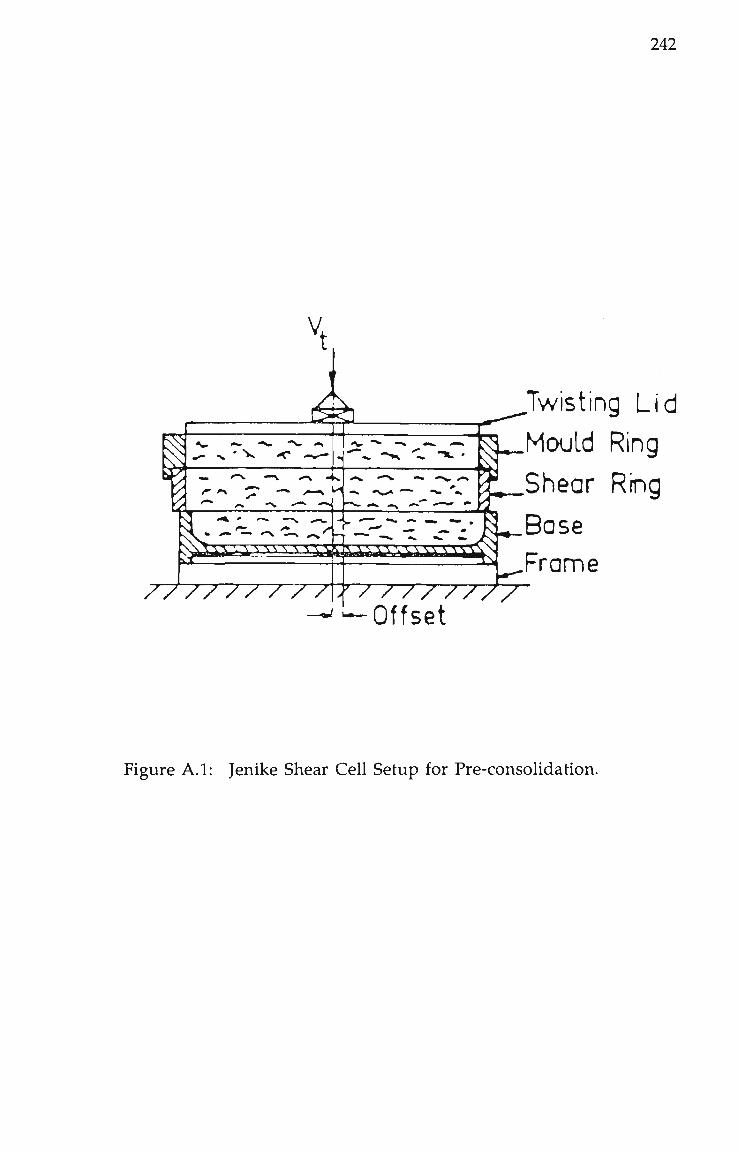
242

P ^ - V ^^

^ _Frame ssss^^^^i^^ssssssssss

/ / / / / / / / /

Twisting Lid

Mcxjld Ring

Shear Ring

7 / / / / / / / / — Offset

Figure A.l: Jenike Shear Cell Setup for Pre-consolidation.

243

excess material level with the top of the mould ring. Cover the sample with

the twisting lid.

Apply a normal vertical force Vj., to the twisting lid by means of a

weight carrier, and, by using the special twisting wrench, apply a number of

oscillating twists (amplitude approximately ± 20 ) to the lid. During this

procedure care should be taken not to press down on the twisting lid and

not to impede the motion of the shear ring as it tends to follow the motion

of the twisting lid.

The selection of the value of Vi and the number of twists to be

applied is determined by trial and error. For most dry samples Vj. is made

equal to V, the normal force used in the consolidation-under-shear

procedure described below. However, for high moisture samples, values of

Vj. equal to 2 to 3 times V may be required. The number of complete twists

applied initially is about 20. The number of twists can be increased to

approximately 40, although this may increase the chance of disturbing the

cell. Altering the number of twists can be considered a method of fine

adjustment rather than altering the value of Vj..

• Remove weight carrier from the twisting lid.

• Lift off mould ring while holding down twisting lid and shear

ring.

• Slide the twisting lid off and scrape the excess material flush with

the top off the shear ring. In these operations care should be taken

to avoid any movement of the shear ring. Clean away excess

material with the brush and be sure that the lid is placed on

sample container to limit moisture loss from the sample. The lid

should not be removed by direct lifting because adhesion of the

coal (particularly at high moisture contents) usually leads to

destruction of the cell compact.

244

A.4.2 Consolidation under Shear

Consolidation of the sample is completed by a shearing operation

which causes the material to flow under the consolidating stresses until a

steady state shear value is reached or closely approached. This is performed

as follows:

• Place the shear lid on the sample taking care to centre it within

the shear ring.

• Apply the force V^ to the lid, using an appropriate weight, and

advance the stem of the Direct Shear Tester against the bracket.

Figure A.2.

• Let shearing proceed until a condition is reached when a layer of

the material across the whole sample is caused to flow plastically

indicated by the recorded shear force reaching a steady value S.

Ideally, this steady value of shear force should be reached when

the shear ring is concentric with the base of the cell because of the

limited travel of the cell arrangement.

• Reverse the stem travel until the shear force drops to zero. Then

remove the force Vj..

It is important that the steady state shear force S is reached as

indicated by curve B, Figure A.3; the sample is then said to be critically

consolidated. If the shear force continues to rise for the complete stem

travel, curve A in Figure A.3, then the sample was under consolidated

during the pre-consolidation phase. Generally, this means that an increase

is needed in the pre-consolidation force Vj. and/or the number of twists

used. If the shear force reaches a maximum then reduces, curve C in Figure

A.3, the sample was over consoUdated during the pre-consolidation phase.

Generally, this means that the value of V^ and/or the number of twists was

excessive.

245

V

a racket 1. ji

/ • - •.. —. .«» .-V •

s -^ >=-

•Offset

^ <i ->./-.. -s-

L^^^'^9 f ^ %~~Frome Sten ////////////////

.Shear L id

Sheer Ring Shear Plane

Figure A.2: Jenike Shear Cell Setup for Consolidation.

A - U n d e r C o n s o l i d a t e d

B - C r i t i c a l l y C o n s o l i d a t e d

C - O v e r C o n s o l i d a t e d

L i m i t of / ^ T r a v e l

S t e m T r a v e l

Figure A.3: Types of Shear Consolidation Curves.

246

A note of caution should be sounded here. The trial and error

procedure (for selecting Vj. and number of twists) should approach the

critically consolidated state from a condition of under rather than over

consolidation. Otherwise it is tempting to over consolidate the sample and

stop the shear consolidation procedure at point X on Curve C in Figure A.3.

Such samples are not critically consolidated and can lead to considerable

error in the resulting yield loci.

A.4.3 Shear of the Sample

The third stage of the test is the actual shearing of the sample

under force Vj, smaller than V. The following is used:

• Apply force Vtj. to the shear lid, using an appropriate weight.

• Advance the stem of the machine until it almost touches the

bracket.

• Let shearing proceed until the recorded pen reaches and passes a

maximum value, Sj.

• Retract stem and remove force V^..

• Remove the entire cell including the shear lid and split the shear

ring and base apart. Check to see that the shear plane is between

the ring and the base and not angled up or down striking the lid

or bottom of the cell. If this has happened the complete test must

be repeated.

Determine the additional vertical force, V^ above the shear plane.

V^ is the vertical force due to:

(i) shear Ud.

(i) shear ring,

(iii) mass of material contained within the ring.

247

This determination only needs to be done occasionally for each

level of consolidation.

A.4.4 Determining the Complete FamUy of Yield Loci

The entire three stage procedure is repeated two more times for

the same level of consolidation, applying the force V ^ to the shear lid

during shear consolidation but applying forces V^ and V ^ to the lid during

shear. A fresh sample of material is used for each test. This set of results will

be used to provide one complete yield locus.

A complete series of tests needs to be performed at two other

levels of consolidation, one higher and one lower than the first level. Thus

the minimum number of valid tests which must be performed to obtain the

family of instantaneous yield loci is nine.

As an example, presented in Table A.l for a coal at 10% total

moisture content are the suggested forces to apply to the shear lid. The force

levels presented may have to be varied slightly to suit particular conditions

and to enable a complete set of valid test results to be obtained. Figure A.4

shows the range of valid points for a yield locus.

It is absolutely essential that the test values are plotted as the tests

proceed to indicate that valid test points are being obtained. Reference is

also made between the yield loci of different yield loci in developing the

family concept and increasing the confidence of the result, and selecting

values for the next test cell.

248

First Series of Tests - Medium Consolidation Level

Shear ConsoUdation V , = 22.6 N (2.3kg)

Sample Shear V^ = 12.8 N (1.3kg)

V|,2= 8.8 N (0.9kg)

V , = 3.9 N (0.4kg)

Second Series of Tests - High Consolidation Level

Shear ConsoUdation V ^ = 31.4 N (3.2kg)

Sample Shear V , = 17.7 N (1.8kg)

Vb2= 12.8 N (1.3kg)

Y^^= 7.8 N (0.8kg)

Third Series of Tests - Low Consolidation Level

Shear ConsoUdation Y^ = 13.7 N (1.4kg)

Sample Shear V^ = 6.9 N (0.7kg)

V^^= 4.9 N (0.5kg)

Vb3= 2.9 N (0.3kg)

Table A.l: Suggested Forces for Shear Testing of Coal

249

^ 1

cd CD

CO

XI •1—1

Val

«fH

m - f j

oin

PU

o •1—1 -(-> (d

O Ti

CD OO a c6

• rH r—1

O w ti o

P^O

CO aoHOJ HvaHS

Figure A.4: Valid Range Points for Instantaneous Yield Locus.

250

A.5 PLOTTING TEST RESULTS TO DETERMINE INSTANTANEOUS

YIELD L O a

When determining a family of yield loci, such as shown in Figure

A.5, it is important that certain fundamental principles be observed when

interpreting the test results.

These can be summarised as follows:

• ensure that the samples have been critically consolidated.

• loci should be drawn as straight lines.

• loci should be parallel or fan out slightly as the normal load (or

stress) increases.

• loci must not intersect.

• the shear consolidation point does not necessarily correspond to

the end point of the yield locus.

• the shear consolidation points generally lie close to a straight line

which either passes through or above the origin.

• the force due to the weight of the shear lid, shear ring and

material contained in the shear ring (V^) must be added to all

vertical forces applied to the shear cover (V^ and V| .) to give the

total vertical or normal force applied to the shear plane.

• the smoothing or prorating procedure of Jenike works well for

instantaneous yield locus test shear force results.

• the yield loci data must fall within the valid range defined in

Figure A.4 and only vary within defined bounds.

• the yield loci can either be plotted in force or stress units. For

convenience it is recommended that force units be used.

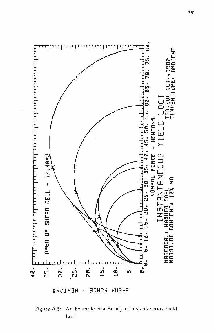
251

• M I I n t > I I I 1 I I I I t I t I 1 11 1 11 n I i l I

63 in s i/> s in s ^ <n n r\j rj «-• -^ m

SN01M3N - 33y0d yb3HS

Figure A.5: An Example of a Family of Instantaneous Yield

Loci.

252

A.5.1 Prorating Procedure

When determining a yield locus, the value of shear force S

obtained during the shear consolidation process will usually show some

scatter. The allowable deviation of S from the intermediate value should be

less than ± 5% and the foUowing relationship [68,69] should be used to

adjust or prorate the raw test results.

(c.\ _ i test selected /• A i \ ^^i^ prorated " S, ^^'^^

^ test

The value of S jg g should be an intermediate value within the

range of scatter of the S ^ ^ values; an average value of all the S ^ ^ values

may be satisfactory. As a guide, when prorating (S.) ^ ^ values for a family of

yield loci, the Sg jg ^ ^ values should lie close to a straight line which passes

through or just above the origin.

A.5.2 Example of Prorating Procedure

The data tabulated in Table A.2 represents a series of yield locus

raw test results for 10% moisture content coal and their subsequent

prorating. The resulting plots of the yield loci ( (V, 5 ^ ^ ^ ) and (Vj,

^ i prorated values for each level of consolidation) are plotted in Figure A.5.

A.6 DETERMINING THE INSTANTANEOUS FLOW FUNCTION

Once the yield loci have been plotted Mohr stress circles can be

drawn for each locus as follows. Figure A.5:

• draw a semicircle, centred on the Normal Force axis, to pass

through the point V, Sg jg ^ j (marked X) and be tangent to the

yield locus. This is referred to as the Mohr circle of flow and

describes the consolidation condition for the locus.

253

• draw a semicircle, centred on the Normal Force axis, to pass

through the origin and be tangent to the yield locus. This is

referred to as the Unconfined Mohr circle and describes the

unconfined strength of the bulk solid for the consolidation level

of the yield locus.

Note that since circles are being drawn on the lYL graph it is

implied that the same scale has been used for the horizontal and vertical

axes.

These Mohr circles provide three combinations of Major

Consolidation Force, V-j and Unconfined Yield Force, F, for the three

members of the yield loci family previously determined. For the example

given in the previous section and the corresponding yield loci plotted in

Figure A.5, these values are presented in Table A.3. These forces can be

converted to stresses by dividing by the cross-sectional area of the shear cell. 1 2 This area is TTJT m for the 95.3mm diameter cell.

This conversion changes

V^ => G^ (major consolidation stress)

F =» o (unconfined yield stress)

and the corresponding values of the example are presented in

Table A.4. These values are plotted in Figure A.6 to provide the

Instantaneous Flow Function. This then quantifies the flow properties of

the material as relevant to short periods of storage.

Generally, the Instantaneous Flow Function can be drawn as a

straight line of best fit through the three plotted points. Alternatively, a

convex upward curve may be drawn. The flow function when extended

should pass through or above the origin of the graph. It will be noted that

the same scale must be used for the horizontal and vertical axes.

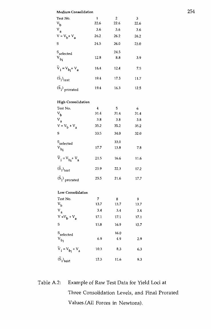
Medium Consolidation 2 5 4

Test No.

\

Va v = Vb+v^

s

g selected

^b i

Vi=Vbi+V^

(Si)test

(S ) 1 prorated

High Consolidation

Test No.

\

Va v = v .+v,

0 a S

selected

^b i

^i = %^v^

(Si)test

(S ) ^ i' prorated

Low Consolidation

Test No.

Vb

Va V =V, + V, b a

S

g selected

bi

V. =V. +V^ 1 Dj a

^^i^test

1 22.6

3.6

26.2

24.5

12.8

16.4

19.4

19.4

4 31.4

3.8

35.2

33.5

17.7

21.5

25.9

25.5

7 13.7

3.4

17.1

15.8

6.9

10.3

12.3

2 22.6

3.6

26.2

26.0

24.5

8.8

12.4

17.3

16.3

5 31.4

3.8

35.2

34.0

33.0

13.8

16.6

22.3

21.6

8 13.7

3.4

17.1

16.9

16.0

4.9

8.3

11.6

3 22.6

3.6

26.2

23.0

3.9

7.5

11.7

12.5

6 31.4

3.8

35.2

32.0

7.8

11.6

17.2

17.7

9 13.7

3.4

17.1

15.7

2.9

6.3

9.3

Table A.2: Example of Raw Test Data for Yield Loci at

Three Consolidation Levels, and Final Prorated

Values.(All Forces in Newtons).

255

Consolidation Level Vj_

High Consolidation 78.9 35.2

Medium Consolidation 58.2 27.9

Low ConsoUdation 37.6 19.1


Instantaneous Flow Function of the Example

(Force Units).

Consolidation Level Oj a^

High Consolidat ion 11,0 4.9

M e d i u m Consol idat ion 8.1 3.8

Low Consolidat ion 5.3 2.7


Ins tantaneous Flow Function of the Example

(Stress Units)

256

T T T I I I I ! I

r

I I I M_ r j

2 to CC

cn ^ CC (L O

, : ^ (D

ox: -•cr

l-UJ OflZ 0 3

h-- a ooc LULU

UJUJ

I -> I 1 I 1 ' ' ' ' ' ' ' ' ' 1¥ > u

I

CO

JD ^ «-J)

O LJ_ I—t

^a g D I »-• u_ -J

o u

tn c o - > a

CD 3 :

ac9 L>

CDt— UJZ XUJ

ccz x o

o -JUJ

ace ect-ujto h-»-« ceo

(O m fo ru

S1d:9bd0"liy - SS3yiS 0131JL 03NUN03Nn

Figure A.6: An Example of an Instantaneous Flow

Function.

257

APPENDIX B

FLOW PROPERTY TEST SAMPLE PARTICLE DISTRIBUTIONS

258

M to flC tu Q X Z3

<n tn CC X

tu o CC

z UJ u OC UJ d.

98.

95. 90.

60. 70. 60. 50. 40.

30.

20. 15.

10.

5.

3.

2.

1.

7"

I

: < ^ :

>;z =i3

- ^

nosiH-nflHMLEn DISTRIBUTIOH COEFF-S SIZE M00Ui.U5 X

X - 4.77»« DISTRIBUTION FRCTOR «

n - .811

1.

5. 10.

20. 30.

50.

100. 10. SIEVE APERTURE - ••

ROSIN-RflMMLER CUMULRTIVE SIZE DISTRIBUTION MRTERIflLi COALCLIFF ROM COAL RS REC 0 TESTEDi 1984 MOISTURE CONTENTi AIR DRIED TEMPERRTUREi AMBIENT

FIOUflEi B.l

Ui

60.

70.

flS oo . 85 .

to CC UJ • ^

o CO «f) OC x

90.

95.

97.

98 .

UJ a CC

z UJ u EC UJ

99.

UJ M

tn CC UJ Q z z> tn tn CC X. UJ C3 a. h-z u UJ

a.

99.

95. 90.

80. 70. B0. 50. 40.

30.

20. 15.

10.

S.

3.

2.

1. /

7

/

.JL

/ ^t %

RDSIN-nHHMLER 0I3TRIBUT10H CQEFF.3

SIZE MOOUi-US X X - . B S M

DISTRIBUTION FRCTOR n - 1-114

.01 .1 SIEVE APERTURE

ROSIN-RRMMLER CUMULRTIVE MfiTERIRLt COALCLIFF ROM COAL -2.3BHM MOISTURE CONTENTI AIR DRIED

FICUBEi B.2

1.

5. 10. 20. 36. 40-50. 60.

70.

80 85.

90.

95.

97.

98.

99.

UJ

.-* tn cr UJ >• o

VI • c t

3C

UJ

u CC

z UJ t J tc lu

1. 10.

s"rZE DISTRIBUTION TESTEDi 1984 TEHPERATUREi AMBIENT

259 99.

SIEVE APERTURE - ••

ROSIN-RRMMLER CUMULRTIVE SIZE DISTRIBUTION !ISfi?flgfe'rSS!/IBT?^kVi KS9en C°"'- f 3 REC'D TESTED, 984

f lCUREi B 3 °^^^'^^ ' " ^ " ° "^^° TEMPERATURE! AMBIENT

09

UJ (»j

tn tc u a z Z3

tn tn a: X

UJ

cr (-z UJ

u CC UI

a.

?i5. 3 0 .

8 0 .

7 0 . R?1. 5 0 .

40 .

3 8 .

2 0 .

15.

10 .

5 .

3 .

? .

1 . . 31

/ /

/ /

/

U- .

/]

/

. 1

/

/

/ r ••'

I -

; <

— - L

^ / ^

/

/

/

ir :

RO; DI3TRI

SIZE M

OISTRI

'

/ C

5IM-nnMHLER aUTIQN CDEFF.S

ODUi.US X

X •• • U 1 M l

BUTION FRCTOR •> n •> 1.419

10

I.

5. 10.

20. 30. 40. 50. 80. 70.

60. 85.

90.

95.

97.

98.

99.

UJ

*-* tn az UJ > •

o v> cn cr z UJ C3 CC »-z UI o QC UJ

a.

»» SIEVE APERTURE

ROSIN-RRMMLER CUMULRTIVE SIZE DISTRIBUTION HflTERIALi SOUTH BULLI PROD. COAL -2.38HM TESTEOi 1984

,.. MOISTURE CONTENTi AIR DRIED TEHPERATUREi AMBIENT FICUREi B 4

UJ M

99.

9 5 . 9 0 .

80. 70. B0. 50. 48.

30 .

260

20.

UJ a z

tn tn cr ^ 15. UJ 13 CC h-Z t j j u a: UJ OL

10.

5 .

3.

2-

I . 1

il Ii

iZ ^

H 10.

2 0 . .39. 4 0 . 5 0 . 6 0 .

79.

80 .

05.

Q0.

ROSIN-RRMMLER OtSTRIBUTION COEFF-S

SIZE MODUi.US X X •• 4 . 4 8 M

DISTRIBUTION FACTOR «| n - .798

95.

9 7 .

9 8 .

9 9 . 100 .

UJ

to OC UJ p-o tn cn CC

s: UJ 13 cr — z UJ o az UJ

1 . 10. SIEVE APERTURE - »a

ROSIN-RRMMLER CUMULRTIVE SIZE DISTRIBUTION MATERIRLi HUNTLET ROM COAL A3 REC'D TESTEDi 1984 MOISTURE CONTENTI AIR DRIED TEHPERATUREi RMBIENT

FICUflEi B.5

as .01 .1

SIEVE APERTURE

ROSIN-RflMMLER CUMULATIVE SIZE DISTRIBUT MATERIALi HUNTLET ROM CORL -2.36MM TESTEDi 1984 MOISTURE CONTENTi AIR DRIED

FIWinEi B.6

ION TEHPERATUREi RMBIENT

261


ROSIN-RRMMLER CUMULRTIVE SIZE DISTRIBUTION IISTI9i'^iSb'rS5lPS?°^IIS^«29SnC°f'L AS RECD TESTEDI 1984

»TriiiiJl°^'J"?^ CONTENTI AIR DRIED TEHPERATUREi AMBIENT ricunEi B.7

99.

95. 90.

80. 70.

ly 60. m 50. <c ._ UJ 40. a i 30. tn n 20. CC

UJ (3 CC »-z UJ u az UJ a.

15.

10.

5.

3.

2 .

1. / 01

, ^ /

/

—

/

... —

/ /

/

. 1

..'^ /

/ /

''

/ r

At.

u / /

/

RO; OlSTRI

SIZE M

OlSTRI

. . •

— Z.: L

5IH-RRMMLER BUTIOH COEFF-S

0DUi.U3 X X • - 4 7 Ml

BUTION FRCTOR • n » i-zas

18

10. 20. 38. 40. 50. 60.

70.

80.

85.

90.

95.

97.

98.

99.

UJ M »-< OT

az UJ > o «r> cn CC

UJ CJ CE »— z UJ

az UJ a.

•« SIEVE APERTURE -

ROSIN-RflMMLER CUMULATIVE SIZE DISTRIBUTION HATERIflLi METROPOLITAN ROM CORL -I.00MM TESTEOi 1984 MOISTURE CONTENTi AIR DRIED TEMPERRTUREi AMBIENT

FlOUREi B 8

262 99.

95. 90.

60. 70.

ut

tn DC UJ

a z =j

tn tn cr z

60. 50. 40.

30.

20. 15.

.01

^

_

/

..

>*"

/

/

. 1

iX ^

/ /

/

/ T

(

-~

V . /

y' /

/ /"•

RO OlSTRI SIZE H

OlSTRI

1 .

/

5IN-RflHMLEB OUTIOH COEFF. ODUJrUS X

X - .87« BUTION FRCTOfl

n - 1-114

. 5 . - 10.

- 20 . - 30 .

50 . ::: cn

- 80. £ - 70. o

in . 8 0 . S - 85. ^

tu

_ 98. E z UJ CJ

a.

5 97 .

, . 98 .

99 . 10.

Ui

g 10. z UJ o _ re 5. a.

3. 2.

1. .01 .1

SIEVE APERTURE - •«

ROSIN-RRMMLER CUMULRTIVE SIZE DISTRIBUTION MATERIALI METROPOLITAN ROM COAL -2.38MM TESTEDi 1984 „„„, .., MOISTURE CONTENTi AIR DRIED TEMPERRTUREi AMBIENT

FIOUREi B.9


ROSIN-RflMMLER CUMULRTIVE SIZE DISTRIBUTION NflTERlV. HETROPOLITRN ROM COAL -4.08MM TESTED. 1984 MOISTURE CONTENTi AIR DRIED TEMPERRrUHti HnoitNi

FICUWi B.IO

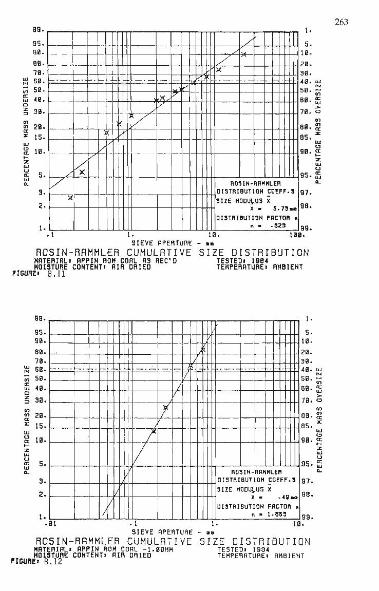
263

.1 1. 10. 100. SIEVE APERTURE - •«

ROSIN-RflMMLER CUMULRTIVE SIZE DISTRIBUTION MATERIRLi APPIN ROM CORL AS REC'D TESTEDi 1984 MOISTURE CONTENTI AIR DRIED TEHPERATUREi RMBIENT

ricmzi B.ll

99.

95. 90.

70. UJ M

cn ir UJ

a z 3 <n tn a X

60. 50.

40. 30.

?n. 15.

UJ u (Z I -z UJ u CC UI 0 .

10.

5.

3.

2 .

1. /

/ /

?•

ROSIM-RRMMLER DISTRIBUTIOH COEFF-S SIZE MODU;.US X

X - . 4 S M

DISTRIBUTION FRCTOR » n • 1-B53

1.

5. 10.

20. 38. 40. 58. 03.

7S.

80.

85.

90.

10.

95.

97.

98.

UJ M -. tn OC bJ > • o tn cn OC 3C

UJ C3 CC •-z lU

o CC UJ

a.

99. .01 .1

SIEVE APERTURE - •«

ROSIN-RRMMLER CUMULATIVE SIZE DISTRIBUTION MATERIRLi APPIN ROM CORL -1.00HM TESTEDi 1984 MOISTURE CONTENTi AIR DRIED TEHPERATUREi AMBIENT

FICUREi B.12

264 99.

95. 99.

80. 70.

^ 60. OT 5 0 . £ 40. o -3 30 . OT OT CZ

z Ui C3 CC t -z UJ u tu a.

20.

15.

10.

5.

3.

2.

1.

I .

01

— —

- - -

<

/ / /

. 1

/

) /

/ "

v / /

/ Ai.

Ro; OlSTRI SIZE M

OlSTRI

1-

1

SIH-HRMMLER BUTION COEFF. ODUi.US X

X « -BSi BUTION FRCTOR

n • 1.187

- 5-- 10.

_ 20 . - 38 .

- 50 . -^ OT

- 80. S _ 70. o

OT

- 80. S - 85. ^

UJ t 3

90 . a:

CO

• iRC

EN

T

a.

5 97 .

^ 98.

99 . 10.

a a SIEVE APERTURE -

ROSIN-RflMMLER CUMULATIVE SIZE DISTRIBUTION MATERIRLI APPIN HOH CORL -2.38HH TESTEDi 1984 MOISTURE CONTENTI AIR DRIED TEHPERATUREi AMBIENT

FIGUREi B.13

ut M » - . OT OC UI Q z r) OT OT CC

z UJ C3 CC h-Z UI o tc tu ft.

gg.

95. 90.

80-70. 60. 50. 40.

30.

20. 15.

10.

5.

3.

2.

I .

/ /

r 7?

A

^/

,^

%

z

nOSIH-RHMMLER DISTRIBUTION COEFF-S

SIZE HODUi-US X X - l - U o a

DISTRIBUTION FRCTOR i n « I .B34

I.

5. 10.

20 . 30. 4 0 . UJ 50. eg.

73.

80 . 85.

90.

95.

97 .

98 .

99.

tn tc UJ >• o OT OT CC

s: l U 13 CC \-z UJ t-3 cc:

10. . 01 • I SIEVE APERTURE - BB

ROSIN-RflMMLER CUMULRTIVE SIZE DISTRIBUTION MATERIALi APPIN ROM COAL -4.00HM I SIISiT.' J f OMBTFUT MOISTURE CONTENTi AIR DRIED TcHPERATUREi RMBIENT

FIGUWEi B.14

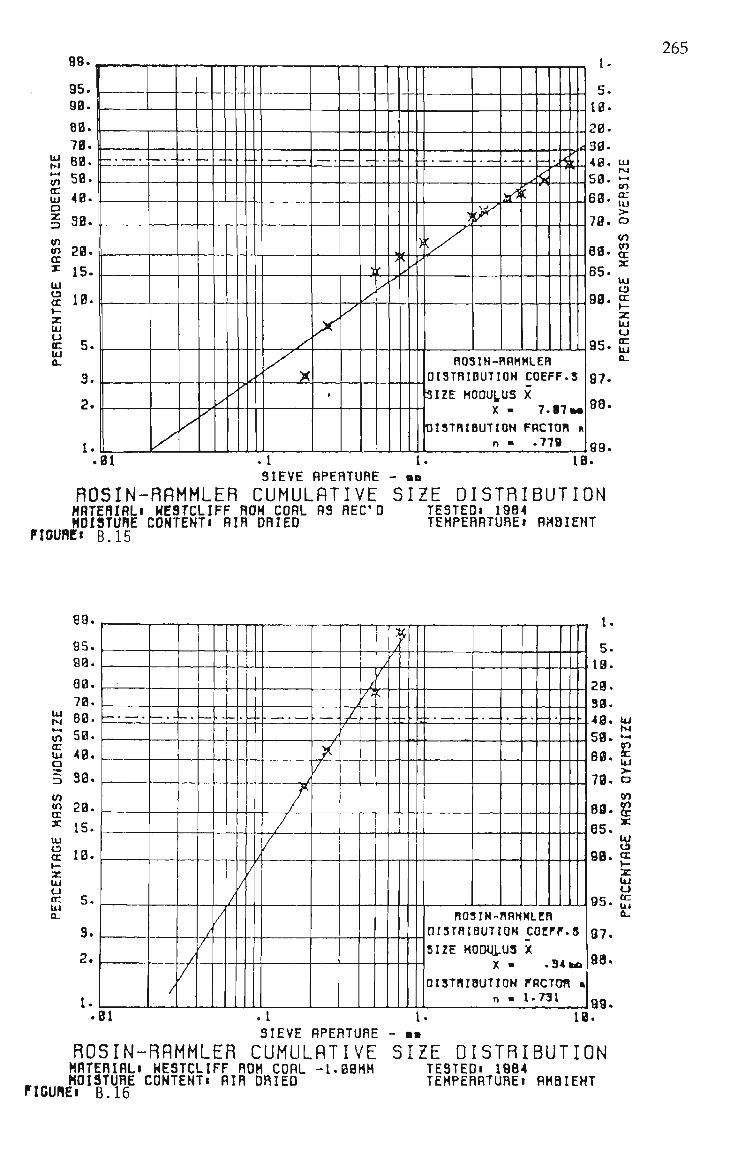
UJ t*J

98.

95. 90.

80. 70 . 60.

cn 50. £ 40. a

-J 30.

OT 20. QC

^ 15. tu t t 10.

265

z UJ u IC UJ a.

5.

3.

2 .

01

X

.1

t

\

r sr'f

s.

M

ROSIM-RRMMLER DISTRIBUTIOH COEFF-S

SIZE MODULUS X

X • 7 - B 7 M i

DISTRIBUTION FRCTOR K n - .778

• . • IB

I .

5. 10. 20 . 30 . 40 50.

. 6 0 .

78.

80.

85.

J99 .

. tu .—. OT o: lu >• o OT OT CE

95.

97.

98.

99.

l U C3 CC t~ z tu CJ

«c lU 0-

SIEVE APERTURE

ROSIN-RflMMLER CUMULATIVE SIZE DISTRIBUTION MATERIRLi WESTCLIFF ROM CORL RS REC'D TESTEDi 1984 MOISTURE CONTENTi AIR DRIED TEHPERATUREi AMBIENT

FIOUREi B.15

89.

95. 90.

00. 70.

lU

OT CC UI Q z OT OT tr z

60. 50. 40.

30.

?0. 15.

UJ t3 CC »-Z lU CJ tn UJ a.

01

/ /

/ /

1

— - -

/ /

/

I

I 1

I ' ' •

/ /

.1

/

/ /

/ / /

/ . / ^

f • / - •

/

^

— T " T * — ' • ' • —

Ro; niSTRI

SIZE H

OlSTRI

, .

- , . - — • - —

. _

SIN-RRHMLER BUTIOH COCFF-

OOMl-US X X - -34

BUTION FRCTOn ry - 1.731

- "

8

M l

IB

10.

5.

3.

2.

1.

SIEVE APERTURE

ROSIN-RAMMLER CUMULATIVE MATERIRLi HESTCLIFF ROM CORL -1.09HH

,.^ MOISTURE CONTENTi AIR DRIED FICUNEi B.16

1.

5. 19.

29. 30. 40. 58 .

80 .

70.

89

85.

QB.

JJJOS.

UJ M

.—*

UJ

>• C3

OT

' "a cr K-Z lU

u tu ft.

97.

98.

99.

• • SIZE DISTRIBUTION

TESTEDI 1984 TEMPERRTUREi RHBIEHT

266

• — •

OT KZ UJ >• O

tu UI CE y~ X Ui o az UJ CL.

SIEVE APERTURE - «B

ROSIN-RAMMLER CUMULATIVE SIZE DISTRIBUTION MATERIAL! HESTCLIFF ROM COAL -2.36HH TESTEDi 1984

„ ^ . MOISTURE CONTENTi AIR DRIED TEMPERRTUREi AMBIENT FICUREi B.17

99.

95. 90.

80. 70.

M 8 0 . m 50. tu 4 0 . a i 30. OT

CC

* 15. lu }? 10. 1 -z UJ

u F. 5-lu

3.

2.

>. . i y

31

/ /

/ /

—

/

/ -

. / ^ / /

.1

^ /

/ /

V

—'

> /'

yi

/ ' l/—-

'T

ROt DISTRI

SIZE M

DISTRI

, , •

—

/ : ^ (—

^ •/'-

.

JIN-RRMMLER nUTIQH COEFF.8

OOUi.US X X - 1 . 1 2 M

BUTION FRCTOn » n - l . N S

IB

1.

5. 18. 29. 30. 43. 50. 80. 7a.

85.

OS.

95.

97.

98.

99.

UJ NI

a

g

• •

FIGU

SIEVE APERTURE -ROSIN-RflMMLER CUMULRTIVE SIZE DISTRIBUTION MATERIRLi HESTCLIFF ROM COAL -4.00HM TESTEDi 1884 NOISTURE CONTENTi AIR DRIED

TOi B.18 TEHPERATUREi AMBIENT

267

18- IBS. SIEVE APERTURE - OB

ROSIN-RflMMLER CUMULRTIVE SIZE DISTRIBUTION MATERIRLi HESTCLIFF PROD. COAL RS REC'D TESTEDi 1984

TEHPERATUREI RHBIEHT MOISTURE FIGUREi B.19

CONTENTI AIR DRIED

99. - , ! •

lU tu OT cn UJ > •

a OT OT

cn

lU ta OC I -z lU o a: tu 0.

SIEVE APERTURE - BB

ROSIN-RRMMLER CUMULRTIVE SIZE DISTRIBUTION MATERIRLi HESTCLIFF PROD. COAL -1.00HH MOISTURE CONTENTi AIR DRIED

FIGUREi B.20

TESTEDi 1984 TEMPERRTUREi AMBIENT

268 89-

95. 90.

80. 70.

OT az UJ a z 3

60. 50. 40.

30.

OT 2 0 . CC X

tu t3 CC \~ z UJ a (C UJ 0 .

15.

10.

3.

2 .

1

i 1

!

1

.01

t

1 - • h • -^ •

i

1

/ /

1 I j

1

[_ 1

/ l/

/

.1

1

/

-^d

. /

/ /

/ i / 1

/1

/ A r

/

[f •-/

ROSIM-RRMMLER DtSTRIBUTIDH COEFF-S

SIZE MODUj;.US X

DISTRIBUTION FRCTOR •> n • 1-533

.. 10

I .

5. 10.

20-30 .

J 4 0 . UJ

59- OT

89- fT;

70.

80-

85-

93.

95.

97.

98 .

99 .

tu

OT

CC

s: tu ta CC V -

z lU t_> tc lu a.

B B SIEVE APERTURE -

ROSIN-RRMMLER CUMULATIVE SIZE DISTRIBUTION MATERIRLi HESTCLIFF PROD. CORL -2.38HM JESTEDi 1984 „„^^^^.^ MOISTURE CONTENTI AIR DRIED TEMPERRTURti AMBIENT

FIGUREi B.21

.01 .1 SIEVE APERTURE - BM

ROSIN-RRMMLER CUMULRTIVE SIZE DISTRIBUTION HATEfllRLi HESTCLIFF PROD. COAL -4.00MH TESTEDi 1984 MOISTURE CONTENTI AIR DRIED TEHPERATUREi RHBIEHT

FIGURE I B.22

269 89.

95. 90-

80. 70.

1 68. OT 50. u 40. a 1 30.

3.

2.

i

/ /

1 i i 1

y

/

/

y • ^

1

/l /

\

r - .

>^^ ^

X-/

..*f. .-

/ 7^'

/ 1 — •

• — L •

ROSIH-RRMMLER OISTRIBUTIOH COEFF-S

SIZE MODULUS X

X •

DISTRIBUTION n "

FRCTOR « .872

1.

s. 10-

20. 30. 40. 50. rr 60.

UJ Ivl

70.

85.

95.

97.

98.

99. .01 . 1 1.

SIEVE APERTURE - BB 10.

ROSIN-RAMMLER CUMULATIVE SIZE DISTRIBUTION M A T E R I A L I HESTCLIFF CORL+FINES-CLAY COHP. TESTEDi 1984 MOISTURE CONTENTI AIR DRIED TEHPERATUREi RMBIENT

FIOUREi B.23

OT

lU

OT OT

cr

tu C3 CC H -

z UJ CJ CC UJ

a.

AH. , 1.

5. 18.

20-38. 48. 53-

60.

70.

80.

85.

98.

95.

97.

80.

99. 1 . 10.

SIEVE APERTURE - BB

ROSIN-RAMMLER CUMULATIVE SIZE DISTRIBUTION MATERIALI HESTCLIFF COAL+FINES- CLAY COHP.TESTEDi 1084

„^, MOISTURE CONTENTI HET SIEVED TEMPERRTUREi AMBIENT FlCUnEi B.24

tu t»j .—. OT tc u a z

OT OT CC

tu o CC H z UJ tJ vc MX

a.

95. 90.

00. 70. R0.

50.

40.

,30.

20.

15.

in.

5.

3.

?.

1. .1 31

X /

.1

W y

y

. _

^ <'

^7'

.)

y \ - ~ - -

Ro; DISTRI

SIZE M

OlSTRI

. , •

^^ f^ - . —

—.,

y*^

. — , . . .

5IH-RRMMLER BUTIOH CDEFF.S

ODUi-US X

X • . 63 KA

BUTION FRCTOR » n >- -sai

10

OT «r UJ > • a OT OT CE 3C

tu ta CC »-z lU o tc tu ft.

270

COMPARISION OF EXPERIMENTALLY DETERMINED FLOW

PROPERTIES

APPENDIX C

INSTANTANEOUS AND TIME FLOW FUNCTION

271

<210

^ 9 i/i UJ

^8

37 UJ

>= 6 D ^ 5 u.

§<* u z => 3

2

1

n

Legend

1 : 2 ! 3 :

-

> < / •

t\^\ ....

Air Dried 10%wb, 15%wb,

1 1

, . . . . ...

{Instantaneous) (Instantaneous) (Instantaneous)

1 1 r 1 1

1

/

1 1

-•^/ V

7 ^

/ _ _ - - ^ ^ ' ' ^

<

1 ^

1

0 1 2 8 9 10 15 MAJOR CONSOLIDATION STRESS - kPa

20

Figure C.l Comparison of Flow Functions for Coalcl i f f ROM Coal (-2.36mni)

0 9 10 15 MAJOU LUN'iULllJAllUN S 1 ULSS - kl>d

Figure C.2 Comparison of Flow Functions for Coalcl i f f ROM Coal (15% wb)

37 UJ

Air Dried (Instantaneous) 6%wb, (Instantaneous) 10*wb, (Instantaneous) 15%wb, (Instantaneous) 15%wb, Time (3 Days)

3-

2-

>S>y <C-y

0 1 2 3 8 9 10 15 MAJOR CONSOLIDATION STRESS - kPa

272

^-^''^^^^^^^^^^''/'^ / ^ ^ -'-' ^ "' ^

'^^^^^^^^ / ^ < ^ ^ ^ ^ ^ ^ ^ '

/ 1 1 1 1 1 1 1 1 1 . 1 1 1

20

Figure C.3 Comparison of Flow Functions for South Bul l i Product Coal (-2.36mm)

alO I

(/I 1/1 UJ

on

UJ

Legend

Air Dried, Instantaneous 6%wb, Instantaneous 6%wb, Time (3 Days) 10%wb, Instantaneous 10%wb, Time (3 Days) 15%wb, Instantaneous 15%wb, Time (3 Days)

W V 10 MAJOR CONSOLIDATION STRESS - kPa

/()

Figure C.4 Comparison of Flow Functions for Huntley ROM Coal (-2.36mm)

273

1 2 3 8 9 10 15 MAJOR CONSOLIDATION STRESS- kPa

Figure C.5 Comparison of Flow Functions fo r Metropolitan ROM Coal (-l.OOmm)

2 3 4 5

Figure C.6 Comparison of Fl

8 9 10 15 MAJOR CONSOLIDATION STRESS- kPa

ow Functions for Metropoli tan ROM Coal (-2.36mm)

274

0 9 10 15 MAJOR CONSOLIDATION STRESS - kPa

Figure C.7 Comparison of Flow Functions for Metropolitan ROM Coal (-4.00mm)

1^10

UJ

^ 8 1/1

UJ

> 6 Q UJ 2

or 2 O u 2 3

0 1 2

• • - r -

Legend

1 : Air Dried 2 : 6%wb, Instantaneous 3 ; 6%wb, Time (3 Days) 4 : 10%wb, Instantaneous 5 ! 10%wb, Time (3 Days) 6 ! lS%wb, Instantaneous 7 ! 15%wb, Time (3 Days)

-

: : ^ _ _ i — 1 1 1 1 1 1 1 1

' — - I •

'^J^'^ - ' < ^ ^ - ^ ^ ^

1

^^^^

1^

1

1

^^'y-^^^'


20

Figure C.8 Comparison of Flow Functions for Appin ROM Coal (-l.OOmm)

275


Fioure C.9 Conparison of Flow Functions for Appin ROM Coal (-2.36mm)

tJlO

^ 9 1/1 UJ

^ 8 on

37 UJ

>= 6 Q

^ 5

u 2 => 5

Legend

Air Dried 6%wb, Instantaneous 6%wb, Time (3 Days) 10%wb, Instantaneous 10%wb, Time (3 Days) 15%wb, Instantaneous 15%wb, Time (3 Days)

0 1 2 6 7 8 9 10 ' 1 5 MAJOR CONSOLIDATION STRESS- kPa

20

Figure C IO Comparison of Flow Functions for Appin ROM Coal (-4.00mm)

276

1 2 3 4 5 6 7 8 9 10 15 MAJOR CONSOLIDATION STRESS - kPa

Figure L . l l Comparison of Flow Functions fo r Westc l i f f ROM Coal (-l.OOmm)

I

i/i UJ

a H

37 UJ

Legend

Air Dr ied 6%wb, I n s t a n t a n e o u s 6%wb, Time (3 Days)

I n s t a n t a n e o u s Time (3 Days) I n s t a n t a n e o u s

10%wb, 10%wb, 15%wb, 15%wb, Time (3 Days)


Figure C.12 Comparison of Flow Functions fo r Westc l i f f ROM Coal (-2.36mm)

277

8 9 10 15 MAJOR CONSOLIDATION STRESS -

Figure C.13 Comparison of Flow Functions for Westcliff ROM Coal (-4.00mm)

ai

UJ ft p

Legend

1 : 6%wb, Instantaneous 2 : 10*wb, Instantaneous 3 : lS%wb, Instantaneous


Figure C.14 Comparison of Flow Functions for Westcliff Product Coal (-0.50mm)

278

!n9 i/i UJ P8 i/i

37 UJ

> 6 0 ^ 5 u.

u z z> 3

2

1

fl

Le

1 2 3

. 4 5 6

-

- /

' ^ <

gend

: 6%wb, : 6%wb, ! 10%wb, : 10%wb, : 15%wb, : 15%wb,

1

I

I n s t a n t a n e o u s Time (3 Days) I n s t a n t a n e o u s Time (3 Days) I n s t a n t a n e o u s Time (3 Days)

r 1 t 1 1

^ ^ ^ ^ ^ ^ ^

1 1

I 7 ' 1 -7 J- 1 ^

y ^ ^ ^^^''"^ j : =* ^ ^ - < : ^ ^'^'^ ^y^^'^^ ^^y^^ ^ - - - j : ; ^ ^ ^ ^ ^

^ ^ ^ ^ ^ ^ : ^ ^ 7

1 1

0 1 2 3 8 9 10 15 MAJOR CONSOLIDATION STRESS - kPa

20

Figure C.15 Comparison of Flow Functions for Westcliff Product Coal (-l.OOmm)

210 j « :

J ,9 1/1 UJ

^ 8 i/i

° 7 - J ' UJ

> 6 Q

^ 5 QI

g 4 LJ 2 ^ 3

2

1

0

Legend

1 ! 2 : 3 : 4 ! 5 ! 6 :

-

^

^^^..^^

^ ^ / . _

6%wb, 6%wb,

10*wb, 10%wb, 15%wb, 15%wb,

^ ^ c J ^

• " ^ ^ ^

—J- 1

• I

I n s t a n t a n e o u s Time (3 Days) I n s t a n t a n e o u s Time (3 Days) I n s t a n t a n e o u s Time (3 Days)

1 1 1 1

^^J;^ ^::^^^^^^

1 1

1 y

^7 ^y

y

1

1 y V A V ^

<.^y O'X

y

1

i^-p-

1 >v.

^ ^ ^ ^ ^ ^ ^ ^

^ * « - ^ ^ ^

-

I

0 1 8 9 10 15

MAJOR CONSOLIDATION STRESS - kPa 20 2 3 4 5 6 7

Figure C.16 Comparison of Flow Functions for Westcliff Product Coal (-2.36mm)

279

£10

Ji9 UJ

^ 8 l/l

q 1

> 6 D

5

-

-

-

-

-

-

legend

1 ! 6%wb, 2 : 6%wb, 3 : 10%wb, 4 : 10%wb, 5 ! 15%wb, 6 ; 15%wb,

1 1 1

Instantaneous Time (3 Days) Instantaneous Time (3 Days) Instantaneous Time (3 Days)

t 1 .1 . 1.

1 y

oy ^y

V

1 1

r

'^y 'y ^'-"""^

"^ .y'''^^

^^''y-^^

• - - ^ ^ ^ ^ ^

J ^ ^ ^ : : : ^ - ^ ^

'

-


20

Figure C.17 Comparison of Flow Functions fo r Westc l i f f Product Coal (-4.00mm)

(Sic I

1/1 (/I UJ CC I -t/i

Q UJ H iZ 2 O u 2

-0.50mm Test Sample (Instantaneous) -l.OOmm Test Sample (Instantaneous) -2.36iraii Tost Sample (Instantaneous) -4.00mm Test Sample (Instantaneous)

1 2 8 9 10 15 MAJOR CONSOLIDATION STRESS - kPa

20

Figure C.18 Comparison of Flow Functions fo r Westc l i f f Product Coal (10% wb.)

280


Figure C.19 Comparison of Flow Functions fo r Westc l i f f Product Coal (15% wb)


Figure C.20 Comparison of Flow Functions fo r Westc l i f f ROM Coal (Tumbled 1 1/2 hours and Remixed -2.36mm)


Figure C.21 Comparison of Flow Functions for Various Coals (-2.36mm, 10%wb)

9 10 15 MAJOR CONSOLIDATION STRESS - kPa

Figure C.22 Comparison of Flow Functions fo r Various Coals (-2.35mm, 15%wb)

282


Figure C.23 Comparison of Flow Functions for Various Coals (10% wb., -2.36mmj


Figure C.24 Comparison of Flow Functions fo r Various Coals (15% wb, -2.36mm)

2 3

Legend

1 : Metropolitan ROM Coal, Instantaneous 2 : Appin ROM Coal, Instantaneous 3 : Westcliff ROM Coal, Instantaneous 4 : Westcliff Product Coal, Instantaneous


20


£10

i/i 9 tn UJ

^ 8 tn

° 7

> 61-

Q

u.

3 -

2 -

1-

-

-

« — - 1 1 I,

1

y^^^"^^

1 I . l . . . . 1

—y

1 1

1

^y yy y

1

v>' y^ 1 y -• 1

y ^>^

^J>-7^^^^^^^

Legend

1 : Metropolitan ROM Coal, Instantaneous 2 : Appin ROM Coal, Instantaneous 3 : Westcliff ROM Coal, Instantaneous

4 : Westcliff Product Coal, Instantaneous

> 1

0 1 8 9 10 15 MAJOR CONSOLIDATION STRESS - kPa

20


284


Figure C.27 Comparison of Flow Functions for Westc l i f f ROM Coal with Bentonite (4.00mm, Various Moisture Contents)

£10

tn tn UJ

I/)

UJ

^ e Q UJ r 2 3 U.

§4 u 2 => :i

9-

1

Legend

.1 : Westcliff ROM Coal (Control) 10%wb Instantaneous

2 : Westcliff ROM Coal (Control) 15%wb Instantaneous

. 3 : Westcliff ROM Coal + Fines, 5%wb. 4 : Westcliff ROM Coal + Fines,10%wb. 5 : Westcliff ROM Coal + Fines,12.5%wb

• 6 : Westcliff ROM Coal + Fines,15%wb.

yj>^

-..'^'^ y ^f^^yy^^"^^

^—' ' ' ' ' 1 ' '

^

1

1

y <^y S^

y/ V

1

7 8 9 10 11 12

&y

y 5;

: Westcliff : Westcliff ! Westcliff : Westcliff : Westcliff : Westcliff

1

6>

ROM ROM ROM ROM ROM ROM

u.

1 ^

^y%^

^^ ^J>^y

Coal Coal Coal Coal Coal Coal

^ ^ 1 yo

+ Kaolin, 5%wb. + Kaolin, 10%wb. + Kaolin, 12%wb. + Bentonite, + Bentonite, + Bentonite,

t

5%wb. 10%wb. 15%wb.

, <:

_


20

Figure C.28 Comparison of Flow Functions fo r Westc l i f f ROM Coal Samples from Free Clay Test Program (-4.00mm)

285

8 9 MAJOR

Figure C.29 Comparison of Flow Clay (-4.00mm,

10 15 CONSOLIDATION STRESS - kPa

Functions for Westcliff ROM Coal Without Free Various Moisture Contents)

9 10 15 MAJOR CONSOLIDATION STRESS - kPa

Figure C.30 Comparison of Flow Functions for Westcliff ROM Coal with Kaolin (-4.00mm, Various Moisture Contents)

286

APPENDIX D

EFFECTIVE ANGLE OF INTERNAL FRICTION

287

8 0 . [••' I ' I • I ' I ' I ' I ' I ' I ' I

in UJ UJ CC o UJ a

40. ' - « • '

0. , I . I . I . I • I • 1 • L _ i — L _ i — L _ J — I — 1 — I • I I — I ' l l — ' • ' • — I

R. 10. 15. 20. 5. 10. 15. MAJOR CONSOLIDATION STRESS - kPo

EFFECTIVE RNGLE OF INTERNAL FRICTION LEGENDi -1- -2.3BHM 10X COALCLIFF

-3- SOUTH BULLI -5- flPPIH -7- HESTCLIFF PnOD.

-2- HUNTLET -4- METROPOLITAN -6- HESTCLIFF ROM

Figure D.l Comparison of 6 for Various Coals (-2.36mm, 10% wb)

n g . I . I . I • I • I I I • I • I • I • I • I ' I ' I ' I ' I ' I ' i ' ' ' ' ' ' '

tn lU UJ CC o UJ a

70.

40. 0.

' • ' • I • I . I — I 1 — 1 L _ i — I — i _ J - ! • • • ' • ' t • I • I • I •

5. 10. 15. MAJOR CONSOLIDATION STRESS - kPo

EFFECTIVE RNGLE OF INTERNRL FRICTION

20.

LEGENDI -I- -2.38HM 15X COALCLIFF -9- SOUTH BULLI -5- APPIN -7- HESTCLIFF PROD.

-2- HUNTLET -4- METROPOLITAN -8- HESTCLIFF ROM

Fiaure D.2 Comparison of 6 for Various Coals (-2.36mm, 15% wb)

GG.

to UJ UJ CC o UJ o

r 70.

60.

50.

40.

-I—'—r

J, . I I I I >

288

- I — I — ' — I — ' — I — ' r - . — I — ' — I — ' — I — ' r - I — I — ' — r - ' — r — ' — I — ' "

0. I . I I I . I . I 1 I I — I — I — I — ' — I — • — ' — ' — 1 — <

5. 10. 15. ' • ' . ' ' I • —

20. HAJOR CONSOLIDATION STRESS - kPo

EFFECTIVE RNGLE OF INTERNRL FRICTION -2- 10X METROPOLITAN -4- 10% HESTCLIFF PROD. -6- 15Z METROPOLITRH -8- 15X HESTCLIFF PROD.

LEGENDi -I- -4.00MM 10X APPIN -3- 10X HESTCLIFF ROM -5- -4.00HH 15X APPIN -7- 15Z HESTCLIFF ROM

Figure D.3 Comparison of 5 for Various ROM Coals (-4.00mm, 10% and 15% wb)

tn UJ UJ tn ta UJ tZi

OS.

70.

40.

-y—t—r-l—r—'—r—1—I—T—r-l—i i i >—|- > i—.—i » i > i • | ' i ' i ' i • • •

' • ' . ' • ' I I 1 I • 1 i _ j 1 1 • ' • ' • 1 . 1

0. 5. 10. 15. HAJOR CONSOLIDATION STRESS - kP»


20.

LEGENDi -1- APPIN -2.38 AD -3- RPPIN 10X

-2- APPIN ex -4- APPIN 15X

Figure D.4 Variation of 6 with Moisture Content (-2.36mm)

289

tn UJ VU CC e j UJ a 1

•o

fit). I ' 'I ' I • I ' I ' I ' I ' I ' ' ' '

70.

I T I I I I I I I I I • I ' I ' I ' '

60.

50.

40.

^°-0^r-^-^^^^^5r-^^-^^"r0. l i '2B. MAJOR CONSOLIDATION STRESS - kPo

EFFECTIVE RNGLE OF INTERNRL FRICTION LEGEND! -1- HESTCLIFF ROM -2-38 AD -2- HESTCLIFF ROM 8X '-^""" _3- SESTCLIFF ROM 10% -4- HESTCLIFF ROM 15X

Figure D.5 Variation of 6 with Moisture Content for Westcliff ROM Coal (-2.36mm)

0 3 . t •. r ' I ' I ' I ' I ' ' ' ' ' ' ' ' ' I ' ' ' ' ' ' ' ' I ' I ' I ' I ' "

m UJ UJ OC o UJ a

50. -

40. _ i . I t . I I 1 • 1 I • I » I > — L . I 1

0. , I • I • ' • ' • • • I • ' • ' • ' • ' '--

10. 15. 28. MAJOR CONSOLIDATION STRESS - kPa

EFFECTIVE RNGLE OF INTERNRL FRICTION LEGENDI -I- HESTCLIFF PROD. 10Z -0.5 -2- HESTCLIFF PROD. -1.00

-9- HESTCLIFF PROD. -2.38 -4- HESTCLIFF PROD. -4.00

Figure D.6 Variation of 6 with Particle Top Size for Westcliff Product Coal (10% wb)

290

tn UJ UJ CC o tu C3

.©

00.

50.

40.

-I— ' — I — ' — r - 1 — I — I — I — . — I — . — r - ' — I — ' — I — ' — r I ' I ' I ' I

' • ' • ' • ' .1 • I • I • J - . I I . I . I I I I • I • 1 i - J

5. 10. 15. 23. MAJOR CONSOLIDATION STRESS - kPa

EFFECTIVE RNGLE OF INTERNRL FRICTION LEGENDi -1- HESTCLIFF PROD. 15X -0.5 -2- HESTCLIFF PROD. -1.00

-3- HESTCLIFF PROD. -2.38 -4- HESTCLIFF PROD. -4.00

Figure D.7 Variation of 6 with Particle Top Size for Westcliff Product Coal (15% wb)

tn tu l U CC a lU a

0 0 . I •• I • I ' I ' I

70.

80.

50.

40.

n—'—I—<—I—'—I" I ' I ' I ' I ' I ' I '

0. > • t . I . I . I t ' • I . I . ' • I • I . I • I • I I I t I » I • I ' ' • J

5. 10. 15. 2a. MAJOR CONSOLIDATION STRESS - kP«

EFFECTIVE RNGLE OF INTERNRL FRICTION LEGENDi -I- METROPOLITAN 10X -1.00

-3- METROPOLITAN 10% -4.00 -5- METROPOLITAN 15X -2.38

-2- METROPOLITAN 10Z -2.38 -4- METROPOLITAN 15X -LOB -8- METROPOLITAN 15Z -4.00

Figure 0.8 Variation of 6 for Metropolitan ROM Coal with Particle Top Size (10% and 15% wb)

291

t n U J U J O C t a UJ a

«3

0 0 . I 1 t I • I I I ' I ' 1 ' I ' I ' I ' I ' ' ' I ' I '

40.

I ' I ' I ' I '

• I • I . ' . ' . I • ' J I I I . I . I . I • I • — I • I • — ' • ' • ' ' ' ' • _

10. 15. 20. B. 5. HAJOR CONSOLIDATION STRESS - kP«

EFFECTIVE RNGLE OF INTERNRL FRICTION LEGENDi -I- QUEENSLAND COAL 10%

-3- HESTCLIFF ROM 10% -5- HESTCLIFF PROD 10%

-2- QUEENSLAND CORL 15X -4- HESTCLIFF ROM 15% -8- HESTCLIFF PROD. 15Z

Figure D.9 Comparison of 6 for Three Coals with Similiar Particle Distributions (-2.36mm, 10% and 15% wb)

tn lU ui CC ID UJ C3

00, r — ' — I ' I ' I ' I ' — I ' I '

70.

i n \ f ' • I 1 I I I — 1 — I — 1

^"'0. 5. I • I I 1 I I I I I

10. 15. I . I

20. MAJOR CONSOLIDATION STRESS - kPa

EFFECTIVE RNGLE OF INTERNRL FRICTION LEGENDi -1- HE3TCLIFF CONTROL 10%

-3- HESTCLIFF TUMBLED 10% -2- HESTCLIFF CONTROL 15% -4- HESTCLIFF TUMBLED 15%

Figure D.IO Comparison of 6 for Westcliff Coal Tumbled and Remixed (-2.36mm, 10% and 15% wb)

tn UJ UJ IE ta UJ o

7R.

60.

50.

40. 0.

I ' r -<—r I ' 1 - r — 1 — r

I I I... • — u ' • I 1 I — I -

I ' I ' I ' I '

I . I • I • I 1.

10. 15. MAJOR CONSOLIDATION STRESS - kPa


20

LEGENDI -I- HE3TCLIFF+FINES -3- HESTCLIFF+DENTONITE 5%

-2- HESTCLIFF+KROLIH 5%

292

Figure D.ll Comparison of 6 for Coal Samples from the Clay Testing Program (-4.00mm, 5% wb)

S s ) . 1—'—I—'—1—'—I—'—r

tn UJ Ui CC ta UI a

MAJOR CONSOLIDATION STRESS - kPtJ

EFFECTIVE RNGLE OF INTERNRL FRICTION LEGENDI -1- HESTCLIFF CONTROL 10%

-3- HESTCLIFF+FINE3 10% -5- HESTCLIFF+KROLIN 10% -7- HESTCLIFF+BENTONITE 10%

-2- HESTCLIFF CONTROL 15% -4- HESTCLIFF+FINES 15% -8- HESTCLIFF+KROLIN VIX -8- HESTCLIFF+BENTONITE 15X

Figure D.12 Comparison of 6 for Coal Samples from the Clay Testing Program (-4.00mm, 10% and 15% wb)

293

APPENDIX E

STATIC ANGLE OF INTERNAL FRICTION

294

86. T—'—I '"I

tn ut UJ tc ta UJ

o

50.

40.

30. I . 1 . 1 . 1 . 1

T — ' 'I •—T"^!—r 1 ' ' ' T — ' — I — < - I ' I — ' — I ' I '

I .. l_ . I . I . I I I » 1 J 1 . I I I 0. 5. 10. 15.

MAJOR CONSOLIDATION STRESS - kPa

STRTIC RNGLE OF INTERNRL FRICTION

20

LEGENDI -1- -2.38MM 10% HUNTLET -3- APPIN -5- HESTCLIFF PROD.

-2- METROPOLITAN -4- HESTCLIFF ROM

Figure E.l Comparison for Various Coals (-2.36mm, 10%wb)

tn tu UI tc ta UI ca


STRTIC RNGLE OF INTERNRL FRICTION LEGENDI -1- METROPOLITAN 10% -1.00

-3- METROPOLITAN 10% -4.00 -5- METROPOLITAN 15% -2.38

-2- METROPOLITAN 10% -2.38 -4- HETROPOLITRN 15% -1-00 -8- HETROPOLITRN 15% -4.08

Figure E.2 Variation of cj) for Metropolitan ROM Coal with Particle Top Size (10% and 15%wb)

295

on. •I ' ' I ' '—I—'—r • t ' I I • T—'—I—'—r - . 1—r—j—.—r-^ ->—I—.—I—.-

tn tu UJ tc ta UI a

50. -

40.

90 . 0 .

• 1 . . I I

5. _!_ . ! _ . 1 1 1 . I I I I I

10. 15. 1 I 1 . . » • I .


STRTIC RNGLE OF INTERNRL FRICTION LEGENDi -1- -2.98MM 15% HUNTLET

-3- METROPOLITAN -5- HESTCLIFF ROM

-2- SOUTH BULLI -4- APPIN -8- HESTCLIFF PROD.

20.

Figure E.3 Comparison for Various Coals (-2.36mm, 15%wb)

to l U UJ CC ta lU

68.

50.

40.

90.

20.

-"—I ' I

•I . 1

I ' I ' I ' I -r-'—r-'—r—'—r

g . . 1 -X -J -X- I . I J i_

- .—I •• I •••—r

5. 10. 15. 1 I I » I .. I.


STRTIC RNGLE OF INTERNRL FRICTION LEGENDi -1- -4.00MH 10% APPIN

-3- 10% HESTCLIFF ROM -5- -4.00HM 15% APPIN -7- 15% HESTCLIFF ROM

-2- 10% METROPOLITAN -4- 10% HESTCLIFF PROD--8- 15% METROPOLITAN -8- 15% HESTCLIFF PROD.

20.

Figure E.4 Comparison for Three ROM Coals (-4.00mm, 10% and 15% wb)

tn U I UJ CC

a UI

0 0 . t - X • I

30.

20 . 0.

T- '—r -.—r—•—r-'—I—>—I—'—I—• I •—I—'—r-l—r

J L J 1 1 1 . — 1 _

T—'—r

5. • I • I • I . I • I i_t I I i_j . I . l . I . l . I . l .

10. 15. MAJOR CONSOLIDATION STRESS - kPo

STATIC RNGLE OF INTERNRL FRICTION

2S.

LEGENDI -1- HESTCLIFF PROD. 10% -1.00 -2- HESTCLIFF PROD. -2.38 -9- HESTCLIFF PROD -4.00 -4- HESTCLIFF PROD. 15% -1.08 -5- HESTCLIFF PROD. -2.38MH -8- HESTCLIFF PROD. -4.08

Figure E.5 Variation of (^t for Westcliff Product Coal with Particle Top Size (10% and'15% wb)

296

tn lU UJ CC t a UJ a

GB.

50.

40 .

30 .

-,—.—I—'—I—1—r -r—J—1 1 1 1—. 1—. I . 1—I I < 1—r- T—'—r

_l__l I . I . I • I . I I . I I I . I

- .—I • I <—r

5. 10. 15. I . I . I I I

20 MAJOR CONSOLIDATION STRESS - kPa

STRTIC RNGLE OF INTERNRL FRICTION LEGENDi -I- APPIN -2-38 8%

-9- flPPIH 15% -5- HESTCLIFF ROM 10%

-2- APPIN 10% -4- HESTCLIFF ROM -2.38 8% -8- HESTCLIFF ROM 15X

Figure E.6 Variation of <^^ for Appin and Westcliff ROM Coal with Moisture Content (-2.36mm)

297

tn ui tu OC ta UI a

G3. I ' I ' I ' I

50.

40.

30. 0.

I . l . I-

-I—' I '—I—'—r -1—'—1—'—1—'—r

. 1 • L-

10. . 1 I l . l l — 1 _

I • r '—I ' I

I . I I I . 1 .. 15. 28

HAJOR CONSOLIDATION STRESS - kP«

STRTIC RNGLE OF INTERNRL FRICTION LEGENDi -1- QUEENSLAND COAL 10%

-3- HESTCLIFF ROM 10% -5- HESTCLIFF PROD. 10%

-2- QUEENSLAND CORL 15% -4- HESTCLIFF ROM 15% -8- HESTCLIFF PROD. 15%

Figure E.7 Variation of (j) for Three Coals with Similar Particle Distributions (-2.36mm, 10% and 15%wb)

tn Ui tu a: ta UJ

a I

5 . J . I I I • I

40.

30.

~ i — ' — I — ' — I — ' — r I ' ' • T — ' — I — ' — r

J .. I I L . l . l l l-

- | — . — I — . — , — 1 — f -

. I I 1 — 1 1 — 1 l — i l _ i I . I . I • I •

0. 5. 10. 15. HAJOR CONSOLIDATION STRESS - kPn

STRTIC RNGLE Of INTERNRL FRICTION

2S.

LEGENDI -1- HESTCLIFF CONTROL 10% -3- HESTCLIFF TUMBLED 10%

-2- HESTCLIFF CONTROL 15% -4- HESTCLIFF TUMBLED 15%

Figure E.8 Comparison of (j)t for Westcliff Coal Tumbled and Remixed (-2.36mm, 10% and 15%wb)

tn Ui Ui CC ts Ui a

58.

40.

30.

298

1—'—I—I—I—.—I—'—I—'—I—'—r 1—'—I' ' I—'—r ^~r

± \ 5. 10. 15. 20 MAJOR CONSOLIDATION STRESS - kPtj

STATIC RNGLE OF INTERNAL FRICTION - 2 - HESTCLIFF+KROLIN 5% LEGENDI - 1 - HESTCLIFF+FINES 5%

- 3 - HESTCLIFF+DENTONITE 5%

Figure E.9 Comparison of (\)i for Coal Samples from the Clay Testing Program (-4.00mm, 5%wb)

tn tu UI tn ta UJ 1:3

60.

50.

40.

30.

2B.

T-' I T-.—\—'—r "T—'—I—<- "1—'—I—'—r-'—r

10. 15. MAJOR CONSOLIDATION STRESS - kPti

STRTIC RNGLE OF INTERNRL FRICTION LEGENDI -1- HESTCLIFF CONTROL 10%

-3- HESTCLIFF+FINES 10% -5- HESTCLIFF+KnOLIN IBX -7- HESTCLIFF+DENTONITE 10%

_L_i 1

23

-2- HESTCLIFF CONTROL 15% -4- HESTCLIFF+FINES 15% -B- HESTCLIFF+KROLIN liX -8- HESTCLIFF+BENTOHITE 15X

Figure E.IO Comparison of (|) for Coal Samples from the Clay Testing Program (-4.00mm, 10% and 15%wb)

299

APPENDIX F

KINEMATIC ANGLE OF WALL FRICTION

300

tu UI CC ta UI C3

10. •1 . • Tl ' I

40. -

30. -

20.

10.

- J — I — I — I — [ — . — I — 1 — I — I — I — I — I — > — I — ' — I — ' — [ — ' t~~' T " ' I ' ' • .

-2.3Q 10% RUSTY MS COALCLIFF -1- : HUNTLET -2- '-

SOUTH BULLI -3- ; METROPOLITAN -4- j

RPPIN -5- : HESTCLIFF ROM -8- I

HESTCLIFF PROD -7- I

"•I ru u-fifa;

' • I . l . I I I 1 I I 1. .._1_ I . I . 1 J_

^

. I . - 1

20. 5. 10. 15. MAJOR CONSOLIDATION STRESS - kPti

KINEMATIC RNGLE OF WRLL FRICTION

Figure F.l Variation of (f) for Various Coals (-2.36mm, 10%wb) on Rusty Mild Steel

tu Ui CC ta lU a

1 — I — I — ' — I ' l l — [ ' I — ' — I ' 1 ' — I ' I ' I • I • r

-2.30 15% RUSTY MS COALCLIFF -1-HUNTLEY -2-

30UTM BULLI -3-HETROPOLITAN -4-

APPIN -5-HESTCLIFF ROM -6-

HESTCL

^~^]

USTCLIFJ PROD -7-

=^i~ = • n = J-rrrf

i_j i_i_j_ j - ^ I • I . ' . I

5. 10. 15. MAJOR CONSOLIDATION STRESS - kP«»

KINEMRTIC RNGLE OF WRLL FRICTION

20.

Figure F.2 Variation of (j) for Various Coals (-2.36mm, 15%wb) on Rusty Mild Steel

301

lU Ui tc ta Ui

a

? fr

50.

40.

30.

20.

10.

-I—I—I—I—I—r 1 ' I ' "1—'—I—'—:—'—r I ' 1 '—r

•rt3 >-

•2.38 10% 304 33 COALCLIFF -1-HUNTLEY -2-

SOUTH BULLI -3-HETROPOLITRN -4-

flPPIN -5-HESTCLIFF ROM -8-

HESTCLIFF PROD. -7-

I . I . I I I I I I . I

0. 5. 10. 15. MAJOR CONSOLIDATION STRESS - kPo

KINEMRTIC ANGLE OF WALL FRICTION

20.

Figure F.3 Variation of cj) for Various Coals (-2.36mm, 10%wb) on 304-2B Stainless Steel

UI tu CC ta UI o

•J. 10. 15.

MAJOR CONSOLIDATION STRESS - kPo

KINEMRTIC ANGLE OF WRLL FRICTION

Figure F.4 Variation of (j) for Various Coals (-2.36mm, 15%wb) on 304-2B Stainless Steel

302

UI tu CC ta Ui a

>

1—[ • I •—r—'—r—'—I ' [ '

•2.38MM 10% PRCTEHE COALCLIFF - 1 -HUNTLEY - 2 -

3QUTH DULLI - 3 -HETADPOLITAN - 4 -

APPIN - 5 -HE3TCLIFF ROM -0-

HE3TCLIFF PROO -7-

MAJOn CONSOLIDATION STRESS - kPo


Figure F.5 Variation of (j) for Various Coals (-2.36mm, 10%wb) on Pactene

I . I I I • I ' — I ' I ' — r ' I ' I ' I - , — I — I > I • — I ' I ' — r ' I

-2.38 15% PfiCTEME COALCLIFF -1-HUNTLEY -2-

30UTH DULLI -3-HETROPOLITON -4-

RPPIM -5-HE3TCLIFF ROM -8-

HESTCLIFF PROD -7-

I I I . I I > .-15. 20.

MRJOR CONSOLIDATION STRESS - kP«i

KINEMRTIC RNGLE OF WALL FRICTION

Figure F.6 Variation of (}> for Various Coals (2.36mm, 15%wb) on Pactene

UI UI OC o Ui ca

50.

40.

30.

20.

1—'—I—'—I—'—I—'—I—'—I—'—I—'—I—'—I—'—I—'—I—'—I—'—I—'—r

APPIN -2.38KM RUSTY MS AD - 1 -nUSTY H3 8% -2-nUSTY M3 10% -3-nUSTT MS 15% -4-

10. _L_i I » t . 1 . I • I 1 I 1 I 1 I • I • 1 I 1



^

I . I

20

Figure F.7 Variation of cj) for Appin ROM Coal (-2.36mm) at Various Moisture Contents on Rusty Mild Steel

303

tii UI CC ta Ui C3

>

,<« . I—'II •—I—'—r

40.

30.

20 .

10. . . i . I I I I

-1—I—I—I—1—I—1—r T—^—r -1—'—I—'—I—'—r

HEST ROM RUSTY H3 AD -l-nU3TT MS 6% -2-nUSTY MS 10% -3-RU3TY MS 15% -4-

I I 1 I I - i — i I I I I i_ I . l - I . l .

0. 5. 10. 15. HAJOR CONSOLIDATION STRESS - kPa


20.

Figure F.8 Variation of (j) for Westcliff ROM Coal (-2.36mm) at Various Moisture Contents on Rusty Mild Steel

304

nq.

40.

lU UI tc to Ui ta 30. -'

20.

10.



Figure F.9 Variation of (j) for Westcliff ROM Coal (-2.36mm) at Various Moisture Contents on 304-2B Stainless Steel

Ui Ui CC a tu ta

HAJOR CONSOLIDATION STRESS - kPo


Figure F.IO Variation of i? for Appin ROM Coal (-2.36mm) at Various Moisture Contents on 304-2B Stainless Steel

305

UI UI tc ta UJ

3 ^



Figure F.l l Variation of cj) for Westcliff ROM Coal (-2.36mm) at Various Moisture Contents on Pactene

50. - ] — i ^ — I — ' — I — ' — I — ' "

UJ UJ CC ta UJ C3

3i

- T - r - r . I . I . I . I ' I ' I ' I ' I ' ' ' ' ' ' ' ' ' .

RPPIN -2.3GMH PACTENE AD - l -PACTENE 8% -2-PRCTENE 10% -3-PACTENE 15% -4-

i s . | . ' • ' i ' • ' i j . ' ' i s r - ^ ' • I • ' •

20 HAJOR CONSOLIDATION STRESS - kPtj


Figure F.12 Variation of tj) for Appin ROM Coal (-2.36mm) at Various Moisture Contents on Pactene

UI Ui (C ta UI CJ

5R. r- '' I ' I ' — I ] — '

40.

30.

20.

1 — ' — r 1 — ' — I — ' — 1 — ' — r ' I ' I

HEST PROD 10% -.5 RUSTY MS -I-

-1.0 RUSTY MS -2-

-2.38HM RUSTY MS -3--4.0 RUSTY H3 -4-

I ' r

10. J • ' • ' ' ' • • I I 1 1 . 1 I I _ l _ i u I • I . • • I . I • I .

0. 5. 10. 15.



28.

Figure F.13 Variation of cf) for Westcliff Product Coal (10%wb) at Various Particle Top Sizes on Rusty Mild Steel

306

UJ UI tc ta UI ta

50.

40.

30.

20.

10. I . 1 . I I I

-T 1 — 1 — I — I 1 — . — I — . 1 — . — I — I — I — I — I — . 1 — . — j — . 1 — r — I 1 I . r

HEST PROD 15% -.5 RUSTY MS -1-

-1.0 RUSTY MS -2-

-2.38 RUSTY MS -3-

-4.0 RUSTY MS -4-

4.»». -tM-

I I I • I I I . 1 I 1 I I . I I I . I I I

0. 5. 10. 15. MAJOR CONSOLIDATION STRESS - V.Pn


23.

Figure F.14 Variation of (}> for Westcliff Product Coal (15%wb) at Various Particle Top Sizes on Rusty Mild Steel

UI UI DC ta UJ

a

50.

40.

30.

20.

- p - . — I — i — I — 1 — I — . — I — i — I — 1 — I — . — I — • — I — . — p - ' — I — . — I — ' — I — ' — I — . — j — ' — I — ' — I — ' I — ' r~^

HEST PROD 10% -.5 PACTENE - 1 --1.0 PACTENE - 2 -

-2.38 PACTENE - 3 --4.0 PACTENE - 4 -

L3j-

10. 0.

' • ' . ' . — I . . . I . t - i _ . 1 . 1 . — I — . -

5. 10. 15. ' . I • I . I '

20. MAJOR CONSOLIDATION STRESS - kPt»


Figure F.15 Variation of (j) for Westcliff Product Coal (10%wb) at Various Particle Top Sizes on Pactene

307

Ui UJ tc ta UJ C3

f ) . I—'—I—'—I—'—I—'—r

40.

30.

20.

10.

T—'—r—1—r—'—I • I

• • I • I . I .._L I I I

I ' I ' I ' I ' I

ENE - 1 - :

-1—I . I • I I I '

HL'ST PnUD ISy. -.5 PnCTENE -1.0 PACTENE - 2 -

-2.38 PRCTENE -3--4.0 PRCTENE - 4 -

^ ^

I . l . ' . '

0. 5. 10- 15-HAJOR CONSOLIDATION STRESS - kP«

KINEMATIC ANGLE OF WRLL FRICTION

I . ' . ' • I • — I

20.

Figure F.16 Variation of (}) for Westcliff Product Coal (15%wb) at Various Particle Top Sizes on Pactene

U i U J t c t a U i c a

50.

40.

30.

" T — ' — I — » — T — ' — I — ' — I — ' — 1 — ' — I — ' — I — ' — I — ' — I — ' — I — ' — I — ' — I — ' — I — ' — I — ' — I — ' — I — ' — 1 — ' — I — ' -

HEST PROD 10% -.5 304 33 -1--1.0 304 33 -2--2.38 304 S3 -3--4.0 304 SS -4-

20.

10. _!_. t.. • I I L I 5. 10.

I . I t I I L

15. I . I » I .,

20 MAJOR CONSOLIDATION STRESS - kPo


Figure F.17 Variation of cj) for Westcliff Product Coal (10%wb) at Various Particle Top Sizes on 304-2B Stainless Steel

308

Ui

w OC ta UI

5. 10. 15. MRJOR CONSOLIDATION STRESS - kPt.


Figure F.18 Variation of (() for Westcliff Product Coal (15%wb) at Various Particle Top Sizes on 304-2B Stainless Steel

309

UJ UJ CC la UJ a

50.

40.

30.

20.

10.

-r—i—1—^

. I I I • 1

j - . - ^ ^ T—'—r'' I T "T—'—I—'—T 1—'-| '—r—'—r—^

RUSTY MS 10% H'LAND -1-RU3TT MS 15% Q'LAND -2-

RUSTY MS 10% HEST. ROM -9-RUSTY MS 15% HEST. ROM -4-

RUSTT MS 10% HEST. PROD. -5-RUSTT MS 15% HEST. PROD. -8-

_. 1 1 I 1 I I I 1 I L _ J • I • ' • I , I . I • ' • I . I



20

Figure F.19 Variation of ^ for Three Coals with Similiar Particle Distributions (-2.36mm, 10% and 15%wb) on Rusty Mild Steel

tu UJ OC la UI o

50.

40.

30.

20.

10

"T—'—I—'—I—'—r -\—'—r "T—'—r—<—I—'—r 1 — ' — I — ' — I — ' — I — • -

304-20 S3 10% Q'LRND -I-304-28 S3 15% 0'LAND -2-

304-28 S3 10% HEST. ROM -3-304-2B SS 15% HEST. ROM -4-

304-28 S3 10% HEST. PROD. -5-304-2B 33 15% HEST. PROD. -8-

. I • I . t . I • I I 1 . .1 I 1 I i _

'0. 5. 10. 15. MAJOR CONSOLIDATION STRESS - kP»


20

Figure F.20 Variation of <p for Three Coals with Simil iar Particle Distributions (-2.36mm, 10% and 15%wb) on 304-2B Stainless Steel

310

Ui tu tc o Ui C3

uo.

40.

- . — I — ' — I — 1 ^ — I ' I — ' — I — ' — I — ' — r

30.

20.

10.

—, p - T — t " - . 1 — r — J — I 1 1 1 1 1 1 — 1 ' I • I '

PRCTENE 10% Q'LAND -1-PRCTENE 15% Q'LAND -2-

PACTENE 10% HEST. ROM -3-PACTENE 15% HEST. ROM -4-

PRCTENE 10% HEST. PROD. -5-PRCTENE 15% HEST. PROD. -0-

J—. L. -i_j U 1 1 I I I I g. 5. 10. 15.

HRJOn CONSOLIDATION STRESS - kPt>


20.

Figure F.21 Variation of <}) for Three Coals with Similar Particle Distributions (-2.36mm, 10% and 15%wb) on Pactene

Ui Ui CC o UJ tzx

50.

40.

30.

20.

10.

I ' I • 1 I ' I ' I ' I " " "T^ T — ' I ' — I • ' I •

I

304-28 S3 10% CON. - l -304-20 33 10% YUMULED -2-

PACTENE 10% CON. -3-PRCTENE 10% TUMBLED -4-304-2B 33 15% CON -5-304-28 15% TUMBLED -8-

PACTENE 15% CON -7-PACTENE 15% TUMBLED -8-

5. l . l l I 1 . 1 I . I I i . I I 1 . I

10. 15. 20 MAJOR CONSOLIDATION STRESS - kP«

KINEMATIC RNGLE OF WRLL FRICTION

Figure F.22 Variation of <p for Westcliff ROM Coal, Tumbled and Remixed, (-2.36mm, 10% and 15%wb) on Pactene and 304-2B

Stainless Steel

UI Ui OC 13 UI a

50. t ' l v , ""

40.

30.

20.

10.

-p-1—I ' I < — I ' I ' I ' I — ' — I ' I ' I ' I ' I ' I

RUSTT MS 10% CON. -1-RU3TY MS 15% CON. -2-RU3TY MS 10% FINES -3-RUSTT MS 15% FINES -4-

I I I

10. I I i_ I I I

15. 20 MRJOR CONSOLIDATION STRESS - kP«


311

Figure F.23 Variation of cf) for Westcliff ROM Coal, Control and Coal + Fines Samples from the Clay Testing Program (-4.00mm, 10%

and 15%wb) on Rusty Mild Steel

UJ Ui CC ta UJ

50.

40.

90.

n— ' I '—r

20.

10*. I . I . I

-I 1—t—r—T—|—r—,—I—j- -.—|—I—r ->—I • r

304-2B 33 10% CON. -1-304-2B 33 15% CON. -2-304-2B 33 10% FINES -9-304-28 SS 15% FINES -4-

I . I I I I 1 I . . 1 . 1 . 1 . I

5. 10. 15. MAJOR CONSOLIDATION STRESS - KPa


20.

Figure F.24 Variation of (j) for Westcliff ROM Coal, Control and Coal + Fines Samples from the Clay Testing Program (-4.00mm, 10%

and 15%wb) on 304-2B Stainless Steel

5 0 . I ' I • I—'— \—>—r

Ui tu tn ta Ui

a

- . — t • ( 1 — 1 • I » -f—^—I ' I ' — r - 1 — I — I I I — I • I

40.

30.

20.

10.

PACTENE 10% CON. -1-PACTENE 15% CON, -2-PACTENE 10% FINES -3-PRCTENE 15% FINES -4-

I I I I I . ' • I • I I I I . j _ i I . I . t I I . I • I . I

5. 10. 15. 20 MAJOR CONSOLIDATION STRESS - kPa


312

Figure F.25 Variation of (j) for Westcliff ROM Coal, Control and Coal + Fines Samples from the Clay Testing Program (-4.00mm, 10%

and 15%wb) on Pactene

UI III tc ta UI

a

50.

40. 7ar

90.

20.

10. . I . 1 . - 1 . i

1 — ' — I — ' — I — ' - I I I I I

RUSTY MS 10% FINES -1-RUSTY MS 15% FINES -2-RUSTT MS 10% BENT. -3-RUSTT MS 15% BENT. -4-RUSTT MS 10% KAOLIN -5-RU3TT MS 15% KAOLIN -8-

=«=*=

I I 1 . I I I -J- I . I I I I I . I . -t I . — I I t_



20.

Figure F.26 Variation of (j) for Westcliff ROM Coal and Added Clays from the Clay Testing Program (-4.00mm, 10% and 15%wb) on Rusty

Mild Steel

Ui tu OC ta tu a

50. 1 — ' — I — ' — I — ' — I — f -

40.

- t3^»y>

30.

20. -

10. I .1... I

"1—'—r—'—I—'—r T—'—r - , — I — i — I — . — I — 1 — I — . —

304-28 33 10% FINES -1-304-28 SS 15% FINES -2-304-2B S3 10% KAOLIN -3-304-28 S3 15% KAOLIN -4-304-28 33 10% DENT. -5-304-2B S3 15% BENT. -8-

I J I l . l l i_ I . I . I . 1

0. 5. 10. 15. HAJOR CONSOLIDATION STRESS - kPa


20.

313

Figure F.27 Variation of (^ for Westcliff ROM Coal and Added Clays from the Clay Testing Program (-4.00mm, 10% and 15%wb) on

304-2B Stainless Steel

UI UJ OC 13 UJ

a

50.

40.

30.

20.

10.

' I ' I ' I ' I I ' I

I

I ' I I ' I

PRCTENE 10% FINES -1-PACTENE 15% FINES -2-PACTENE 10% KAOLIN -3-PACTENE 15% KAOLIN -4-PACTENE 10% BENT. PACTENE 15% DENT. -8-

1.. 1 . l . l l . 1 . 1 . I I I



I I 1

20.

Figure F.28 Variation of <t> for Westcliff ROM Coal and Added Clays from the Clay Testing Program (-4.00mm, 10% and 15%wb) on Pactene

314

APPENDIX G

BULK DENSITY

315 1200. I I i 1 1 • 1 1 1 1 I I 1 1 I ,

1100.

tn

X 1000. 5C

tn 2: UJ a

oa

900.

800.

700.

• ' ' I ' ' ' ' I ' ' ' • I ' I ' I I ' . . • I • . I • 1 1 I » I I I i I I 1 1

8 0 0 . J • • • ' • ' ' ' ' . ' . • ' ' ' • • • • ' I •• 11

0. 25

MAJOR CONSOLIDRTIGN STRESS ~ kP»

BULK DENSITY LEGENDI -1- HUNTLEY -2.38HH 10% -2- SOUTH BULLI -2.38HH IBX

-3- APPIN -2.38MM 10% -4- METROPOLITAN -2.38MH 18% -5- HFSTCLIFF ROM -S-SSHH 10% -B- HESTCLIFF PROD -2.38MM 18%

Figure G.l Comparison of Bulk Density Variations for Various Coals (-2.36mm, 10%wb)

to a

to a: UJ Q

l a

m


BULK DENSITY LEGENDI -1- COALCLIFF -2.38HM 15% -2- HUNTLEY -2.98MH 15%

-9- SOUTH BULLI -2.38MM 15% -4- RPPIN -2.38MM 15% -5- METROPOLITAN -2.38MM 15% -8- HESTCLIFF ROM -2.38MM 15% -7- HESTCLIFF PROD -2.38HM 15%

Figure G.2 Comparison of Bulk Density Variations for Various Coals (-2.36mm, 15%wb)

75.

316

25. 50. MRJOR CONSOLIDATION STRESS - kPo

BULK DENSITY

75.

LEGENDi -1- HESTCLIFF PROO -1.00MH 15%-2- HESTCLIFF PROD -2.36HM 15% -3- HESTCLIFF PROD -4.00MH 15%-4- HESTCLIFF PROD -D.50MM 15%

Figure G.3 Comparison of Bulk Density Variations for Westcliff Product Coal (15%wb) at Various Particle Top Sizes

1000.

cn

900. -

800.

tn

S 700. a

ZD CD

600.

500.

T-r't'T Y * ' '~T I ^ - n T y r r - T T y r~r' yr^ T r y t r r r I T T T-| f i - T i r TT'T T r}-r i T T-pT T T' r ]• TT > r |

• ' ' ' • * t « ^ » i i t i i i t t t l \ t * % t l l t t t l % t * l l t l f t \ t t t l l k A t \ t ^ » M t t t l % A » i i t t A t ^ t » j


BULK DENSITY

75.

LEGENDi -1- HESTCLIFF PROD -1.00MH 10%-2- HESTCLIFF PROD -2.98MH IBX -3- HESTCLIFF PROD -4.00MM 10%-4- HESTCLIFF PROD -0.5BHH 10%

Figure G.4 Comparison of Bulk Density Variations for Westcliff Product Coal (10%wb) at Various Particle Top Sizes

317

tn M

I

>-

1200.

1100.

1008.

tn

5 900. C3

- J r3 tn

800.

700.

' ' ' ' ) ' '' ' I I ' ' ' I I i I • I [ I r • ' I ' • . ' I ' ' ' ' I ' ' ' ' I ' ' • ' I I ' I . I T I I I I I I I I I . I I I ( I I I I I

' ' ' ' ' ' ' ' ' ' ' ' ' ' • ' ' • ' • I ' ' ' ' • • • ' . ' ' ' ' ' I ' . . . I • . • • ' • • • 1 I . . . . < • . . . I . . . . I . . . . I .

25. 50. 75 MRJOR CONSOLIDATION STRESS - kPa

BULK DENSITY LEGENDi -1- HUNTLEY -2.38MH RD

-9- HUNTLEY -2.38MM 10% -2- HUNTLET -2.96HH 8% -4- HUNTLET -2.3BHM 15%

Figure G.5 Comparison of Bulk Density Variations for Huntley ROM Coal (-2.36mm) at Various Moisture Contents

UB0.

700.

vi-fy-^^T-t-y f r 1 r ^ rt -r T |"r"i"T-T-TT r r T ] T T T T y T t T-» | T T r T y r * T T t-rt ir ^-f T-T T J I"I ••-TY-rT'VT f-r ri •*-

0- 25. 50. 75. MAJOR CONSOLIDATION STRESS - kPe

BULK DENSITY LEGENDi -I- SOUTH BULLI -2.38HM RD -2- SOUTH BULLI -2.98HM 8%

-3- SOUTH BULLI -2.38MH 10% -4- SOUTH BULLI -2.38MH 15%

Figure G.6 Comparison of Bulk Density Variations for South Bulli Product Coal (-2.36mm) at Various Moisture Contents

318

l l 8 9 * r" '*- " frr r-y-'i r T r i 7 1 i i T |

1888.

to 3

300.

^ . T ' I I 1 . r I I I I • I I I I I > r I T I I j 1 I f . ; 1 1 I I I I I . . ] ' ' . '

tn

?. 8B8. Ci

tn

700.

Q o a t . • • . < . . . • I • . • • I • • • • 1 • • • • I . • • . I . ' . • 1 . ' . . 1 . . . • ' • ' « . 1 ' I ' ' < I • . ' 1 1 • I ' 1 ' . ' ' I • • • ' _

^^"'0 . 25. 50. 75. MRJOR CONSOLIDATION STRESS - kPa

BULK DENSITY LEGENDi -1- APPIN -4.80MM RD

-9- RPPIN -4.00HM 10% -2- RPPIN -4.00MM 6% -4- APPIN -4.08HM 15%

Figure G.7 Comparison of Bulk Density Variations for Appin ROM Coal (-4.00mm) at Various Moisture Contents

tn •

I

> -

1000.

tn

£ 900. a

= j 03

1 2 0 0 . I . I • I T ' ' I ' I ' ' ' ' I ' ' ' ' M ' ' ' I ' ' ' ' I ' ' ' ' I ' ' ' ' I ' ' ' ' I ' ' ' ' I ' ' ' ' ' ' ' ' ' ' ' ' ' ' ' ' ' ' ' ' ' ' ' '

1100.

000. -

700. . 1 . . . . I . . . . 1 . . X . 1 . . I . I 11 I 1 I I I I I I . I I I I I I I I I > . . . I • . • I I I . > I I . . t . I . . f

0. 25. 50. 75. MAJOR CONSOLIDATION STRESS - kPa

BULK DENSITY LEGEND! -1- METROPOLITAN -4.00MM AD -2- METROPOLITAN -4.00MM 8%

-9- METROPOLITAN -4.00MM 10% -4- METROPOLITAN -4.B0MH 15%

Figure G.8 Comparison of Bulk Density Variations for Metropolitan ROM Coal (-4.00mm) at Various Moisture Contents

319

1000.

S00. oo

I

tn z UI a

800.

m 700.

f r-> T ^ ? » 1-T y T-f I r y T-f T-»-*-T r t T' r? »-r > y r t T T p r i - i T-prTT-f-y-T • o r-^-yi i t y i-f r i ^ - r r r f ; r r i 17' •• r-rT

600. 0.

. * f f l ' * ' ' * * ' ' * * ' f ' ' * * * ' ' ' ' * ' ' * 1 ' ' * ' -t, >J-1 » J » 1.1 t I 1,1 > 11..* 1 I..I I I, 1 « 4.t 1.A I l-I *-l.*..*.*^


BULK DENSITY

75.

LEGENDi -1- HESTCLIFF PROD REMIX 10% -2- HESTCLIFF ROM REMIX 18% -9- QUEENSLAND COAL REMIX 10%

Figure G.9 Comparison of Bulk Density Variations for Three Coals at Similiar Particle Distributions (-2.36mm, 10%wb)

l c 0 0 . r ' ' ' I I' . ' I' ' I . " . I 1'^ I I . . I . I I

tn fl

tn z UJ a

r3

1100.

1000.

900.

800.

700.

I ' ' ' ' I ' I • • I ' ' ' ' 1 ' " I " ' ' T~T'T'r~T T T- T T I ' ' ' ' ! ' ' * '

0. . 1 1 1 1 . 1 1 1 1 1 . . I • . . . 1 • 1 . . I J . 1 . 1 . . . • 1 . . . . I . . . . 1 . . • • I


BULK DENSITY

i i t i i > t t t t » . « i i t * t t |

75.

LEGENDI -1- HESTCLIFF PROO REMIX 15% -2- HESTCLIFF ROM REMIX 15% -9- QUEENSLAND COAL REMIX 15%

Figure G.IO Comparison of Bulk Density Variations for Three Coals at Similar Particle Distributions (-2.36mm, 15%wb)

1100.

1000.

900.

tn ^ 800. C3

tn

03

700.

320

y-^'i r y ^ ^ r t -^ »'i r r yr y-f T-yr r T r-r-r T r-r- ] T-T T T-y-r-TT > y T i T r- y-r T i r T T r f T y T i T T ' y r - T T T pT'T t t j T » T-t

Q Q Q , ! . » > » • I - « * * « ^ < * ^ i « « l t i » t l » . i * l i t » i . l i t . . 1 > i t i t « t f .

0. i.fc. t.l.LjLJLLa..J

25. 50. MAJOR CONSOLIDATION STRESS - kPo

BULK DENSITY

75.

LEGENDi -I- HESTCLIFF TUM i REMIX 10% -2- HESTCLIFF TUM 4 REMIX 15% CON -3- HESTCLIFF TUM t REMIX 15%

Figure G.ll Comparison of Bulk Density Variations for Westcliff ROM Coal, Tumbled and Remixed (-2.36mm, 10% and 15%wb)

1200.

1100.

tn a ca

i(Z

I

> -

CO z UJ o

Z3

1000.

300.

600.

700.

600.

I . I I i I I I I r ' l I I I I I I 1 f > [ I 1 . I [ I I I f I I I I I I I I I I I ' I ' . I ' ' ' I I • ' ' ' I • ' ' ' • ' • • • '

I . . . . I 1 . . . . I . . . . I . . • • 1 1 . I I I . I l l I I I I I I • I I I I I I . . I • I • I I I • I I

25. 50 . MAJOR CONSOLIDRTIGN STRESS - kPo

BULK DENSITY LEGENDI -1- HESTCLIFF CON 10%

-9- HESTCLIFF+FINES 5% -5- HE3TCLIFF*FINE3 12.7%

-2- HESTCLIFF CON 15% -4- HESTCLIFF+FINES 10% -8- HESTCLIFF+FINES 15%

75.

Figure G.12 Comparison of Bulk Density Variations for Westcliff ROM Coal, Control and Coal + Fines Samples from the Clay Testing Program (-4.00mm) at Various Moisture Contents

321

cn n

i2s^n.

1100 .

1000 .

>->--

tn z ui a

ca

sm.

808.

700.

600.

• 7 T-T-T-T • f I r » I J -T ' p r r r-r~f~r r T T -pr ? -T-T T I I I ( T T 1 r ] f I I T J I 1-1 T T ^ I T I

25 . 50 . 75 MflJOfl CONSOLIORTIOH STRESS - kPe

BULK DENSITY LEGENDI -1- HESTCLIFF CON 10%

-9- HESTCLIFF+KROLIN 10% -2- HESTCLIFF+FINES 10% -4- HESTCLIFF+BENTONITE 10%

Figure G.13 Comparison of Bulk Density Variations for Westcliff ROM Coal and Added Clays from the Clay Testing Program

(-4.00mm, 10%wb)

1 2 0 ? ! . ( ' ' ' ' r ' ' •• - f ' ' • ' 1 • • - • 1

1100.

tn .1

>-1 -.~ • (/) T. UI

CQ

1000.

900.

800.

708.

t ^ r T- r T 1 r-T- T -f~T- r r ; * t r 1 j 1 i ' T y f-< t T-J T T T r y T T-r -T- | T T-»- >-

LA.f, i t l l f l ^ l t i t 1 ^ 1 1 t l t I f I ll t J f 1 ' I t ' i i i i I J 1 1 A t i t - l t J - l J ^ J « t J

0. 25. 50. HAJOR CONSOLIDATION STRESS - kPo

BULK DENSITY

75.

LEGEND! -I- HESTCLIFF CON 15% -3- HESTCLIFF+KROLIN 12%

-2- HESTCLIFF+FINES 15% -4- HESTCLIFF+BENTONITE 15%

Figure 0.14 Comparison of Bulk Density Variations for Westcliff ROM Coal and Added Clays from the Clay Testing Program

(-4.00mm, 15%wb)

322

APPENDIX H

SUMMARY OF CRITICAL MASS FLOW HOPPER GEOMETRY

PARAMETERS

Table H.l: Summary of Mass Flow Hopper Geometry Parameters for Coalcliff ROM Coal, for Various Moisture Contents and Sample Particle Top Sizes

Wall Material Instantaneous

Conditions

c c

(deg.) (mm.) "p

(deg.) \

(mm.)

-2.36mm Test Sample, Air Dried

Rusty Mild Steel


Pactene

4.0 25

4.5 25

» »

14.0

15.0

»

15

15 *

-2.36mm Test Sample, 10% w.b. Moisture Content

Rusty Mild Steel


Pactene

* *

21.0 870

12.5 770

»

30.0

21.5

»

385

370

-2.36mm Test Sample, 15% wb. Moisture Content

Rusty Mild Steel


Pactene

8.5 870

22.0 1050

18.0 990

17.5

31.5

27.5

430

460

450

-l.OOmm Test Sample, 15% wb. Moisture Content

Rusty Mild Steel


Pactene

3.5 900

20.0 1185

11.0 1020

13.0

28.5

20.0

470

505

485

Critical Parameters are governed by wall friction considerations and particle interlocking rather than cohesive arching.

323

Table H.2: Summary of Mass Flow Hopper Geometry Parameters for

South Bulli Product Coal (-2.36mm Test Sample).


Conditions

«c ^c «p \

(deg.) (mm.) (deg.) (mm.)

TimeStorage

Conditions (3Days)

«ct ^ct «pt \ t


Air Dried

Rusty Mild Steel


Pactene

* * 8.5 60

1.5 110 14.0 60 » * » »

-

-

.

-

-

-

6% w.b. Moisture Content

Rusty Mild Steel


Pactene

4.0 725 13.5 375

21.0 880 31.0 410

20.5 875 31.5 410

-

-

.

-

-

-


Rusty Mild Steel


Pactene

5.5 895 15.0 455

22.0 1085 31.5 495

21.5 1080 32.0 49

-

-

.

-

-

-


Rusty Mild Steel


Pactene

5.0 1285 14.5 660

23.5 1520 34.0 725

19.0 1460 29.5 705

5.5 1435 15.0

24.0 1720 35.0

19.5 1645 30.0

735

810

790

Critical Parameters are governed by wall friction considerations

and particle interlocking rather than cohesive arching.

324

Table H.3: Summary of Mass Flow Hopper Geometry Parameters for Huntley ROM Coal, (-2.36mm Test Sample)


Conditions «^ B^ a B„ c c p p


TimeStorage

Conditions (3Days)

"ct

(deg.)

\ t

(mm.) "pt \ i

(deg.) (mm.)

Air Dried Moisture Content

Rusty Mild Steel


Pactene

3.5 120 13.5 65

19.5 140 29.5 70

10.0 130 20.0 65

-

-

-

-

-

-

-

-

-

-

-

-


Rusty Mild Steel


Pactene

1.5 605 11.0 320

18.0 735 27.0 345

22.0 775 33.5 355

3.5

21.5

22.5

870

1130

1150

13.0

31.0

33.5

455

500

505


Rusty Mild Steel


Pactene

4.5 1135 14.0 585

23.5 1395 34.0 645

19.0 1330 29.5 63

15% w.b. Moisture Conten

Rusty Mild Steel


Pactene

2.5 755 12.0 400

24.0 935 35.0 445

18.0 885 28.0 430

5.0

24.5

19.5

1305

1645

1550

14.5

35.0

30.0

670

740

720

3.0

25.0

19.0

910

1130

1065

12.5

36.0

29.5

480

535

515

325

Table H.4: Summary of Mass Flow Hopper Geometry Parameters for Metropolitan ROM Coal (10% w.b. Moisture Content)


Conditions

«c

(deg.)

\ «P \

(mm.) (deg.) (mm.)

TimeStorage

Conditions (3Days)

«ct

(deg.)

«ct

(mm.) V «ct

(deg.) (mm.)

-l.OOmmTest Sample

Rusty Mild Steel


Pactene

3.0

9.5

16.0

815 12.5 425

900 17.5 435

985 25.5 455

5.0

19.5

18.0

1480

1955

1900

14.0

27.5

28.5

755

805

810

-2.36mm. Test Sample

Rusty Mild Steel


Pactene

6.0

18.0

18.0

930 15.5 475

1065 27.0 500

1070 28.5 505

7.0

22.0

20.0

1465

1815

1760

16.5

32.0

30.5

735

795

790


Rusty Mild Steel


Pactene

9.0

24.0

19.5

860 19.0 435

990 34.5 465

950 30.0 455

9.5

26.0

21.0

1220

1435

1370

19.5

37.0

32.0

615

665

650


Metropolitan ROM Coal (15% w.b. Moisture Content)

326


Conditions

«c

(deg.)

Be "p Bp

(mm.) (deg.) (mm.)

TimeStorage

Conditions (3Days)

«ct

(deg.)

Set

(mm.)

«pt \ t

(deg.) (mm.)

-l.OOmmTest Sample

Rusty Mild Steel


Pactene

4.5

10.0

9.5

660 14.0 335

745 17.0 340

735 17.0 340

6.0

20.5

17.5

1710

2345

2175

15.5

29.5

27.0

840

900

890


Rusty Mild Steel


Pactene

6.5

20.5

17.0

800 16.5 405

940 30.5 435

905 27.0 430

7.0

21.5

18.0

935

1105

1060

16.5

31.5

28.0

475

510

500


Rusty Mild Steel


Pactene

2.5

21.5

18.5

565 12.0 295

690 32.0 325

665 28.5 320

4.5

23.5

19.5

755

915

880

14.0

34.0

30.0

390

430

4201

327


Appin ROM Coal (6% w.b. Moisture Content)


Conditions

«c

(deg.)

B„ a„ B„ c p p

(mm.) (deg.) (mm.)

TimeStorage

Conditions (3Days)

«ct

(deg.)

\ t

(mm.) "pt «ct

(deg.) (mm.)

-l.OOmmTest Sample

Rusty Mild Steel


Pactene

»

»

1.5

* 5.5 195 * * »

375 12.5 200

»

»

10.5

*

*

620

8.0 *

20.0

290 »

310


Rusty Mild Steel


Pactene

4.0

14.0

16.5

530 13.5 275

585 22.5 285

600 26.0 290

4.5

18.0

18.0

705

805

805

14.0

27.5

28.0

365

390

390


Rusty Mild Steel


Pactene

5.0

19.5

20.0

645 14.5 335

745 29.0 355

750 30.5 360

5.5

20.5

20.5

720

840

835

15.0

30.5

31.0

370

400

400

Critical Parameters are governed by wall friction considerations

and particle interlocking rather than cohesive arching.

328




Conditions

«c

(deg.)


(mm.) (deg.) (mm.)

TimeStorage

Conditions (3Days)

«ct

(deg.)

\ t

(mm.)

«pt \ i

(deg.) (mm.)

-l.OOmmTest Sample

Rusty Mild Steel


Pactene

5.5

20.0

15.0

1520 15.0 780

1755 30.5 840

1670 25.0 820

6.0

21.5

15.5

1815

2105

1995

16.0

32.0

26.0

930

1000

975


Rusty Mild Steel


Pactene

5.5

21.0

15.5

845 15.0 435

1005 31.0 470

945 25.0 455

6.5

22.5

16.5

1065

1270

1195

16.0

33.0

26.5

540

590

570


Rusty Mild Steel


Pactene

6.0

20.0

16.0

850 15.5 435

980 30.0 465

940 26.5 455

6.5

21.0

17.0

980

1145

1100

16.0

31.5

27.0

500

540

530

329

Table H.8; Summary of Mass Flow Hopper Geometry Parameters for



Conditions

«c

(deg.)

\ «p \ (mm.) (deg.) (mm.)

TimeStorage

Conditions (3Days)

«ct

(deg.)

\ t

(mm.)

«pt \ t

(deg.) (mm.)

-l.OOmmTest Sample

Rusty Mild Steel


Pactene

5.0

20.5

16.0

1625 14.5 830

1910 30.5 895

1825 26.0 875

5.5

21.5

16.5

1920

2240

2135

15.0

31.5

27.0

985

1060

1035


Rusty Mild Steel


Pactene

7.5

23.5

16.5

1140 17.0 580

1305 34.0 625

1230 26.5 605

7.5

24.0

17.0

1340

1535

1450

17.5

35.0

27.5

685

740

715


Rusty Mild Steel


Pactene

7.0

23.0

16.5

1065 16.5 545

1220 33.5 585

1155 27.0 570

9.0

24.5

18.5

1500

1735

1640

18.5

35.5

29.0

755

820

795

330


Westcliff ROM Coal (6% w.b. Moisture Content)


Conditions

«c

(deg.)


(mm.) (deg.) (mm.)

TimeStorage

Conditions (3Days)

«ct \ t

(deg.) (mm.) V \ i

(deg.) (mm.)

-l.OOmmTest Sample

Rusty Mild Steel


Pactene

2.5 K-

18.5

52 12.0 275

* 6.5 270

615 29.0 300

4.0 925

7.5 960

19.5 1085

14.0

17.0

30.5

480

490

520


Rusty Mild Steel


Pactene

1.5

7.5

22.0

530 11.0 280

565 16.5 285

660 33.5 310

3.0 690

12.5 765

22.5 850

12.5

21.5

34.0

360

375

300


Rusty Mild Steel


Pactene

5.0

16.5

21.5

680 14.5 350

770 25.5 370

810 32.5 380

5.5 770

17.5 885

21.5 925

15.0

27.0

32.5

395

420

430

331




Conditions

«c

(deg.)


(mm.) (deg.) (mm.)

TimeStorage

Conditions (3Days)

«ct

(deg.)

\ t

(mm.) "pt

(deg.) (

«ct

mm.)

-l.OOmmTest Sample

Rusty Mild Steel


Pactene

4.0

20.5

19.0

1630 13.5 835

1975 29.5 900

1945 29.5 900

4.5

22.0

19.0

1985

2440

2365

14.0

31.5

30.0

1015

1105

1095


Rusty Mild Steel


Pactene

7.0

22.5

20.5

1145 16.5 575

1375 32.0 620

1345 31.0 615

7.5

23.5

21.0

1455

1745

1695

17.0

34.0

32.0

735

795

785


Rusty Mild Steel


1 Pactene

9.5

24.0

20.5

1240 19.5 625

1425 34.5 625

1380 31.0 655

10.0

25.5

21.0

1680

1940

1870

20.0

36.5

32.0

845

910

8951

332

Table H.l l : Summary of Mass Flow Hopper Geometry Parameters for



Conditions

«c

(deg.)

«c «p \ (mm.) (deg.) (mm.)

TimeStorage

Conditions (3Days)

«ct

(deg.)

\ t

(mm.) V

(deg.) (

«ct

mm.)

-l.OOmm. Test Sample

Rusty Mild Steel


Pactene

6.5

23.0

16.5

1820 16.0 925

2130 32.5 1000

2010 26.5 970

7.0

23.5

17.0

2005

2360

2220

16.5

33.5

27.0

1015

1100

1065


Rusty Mild Steel


Pactene

6.0

21.0

17.0

1265 15.5 645

1440 31.0 695

1390 27.5 685

7.0

22.5

18.0

1575

1815

1745

16.5

33.0

28.5

805

865

850


Rusty Mild Steel


Pactene

5.0

26.0

18.5

1120 14,5 580

1340 37.0 640

1260 28.5 615

6.0

26.5

19.0

1280

1535

1440

15.5

38.0

29.5

655

725

700

333


Westcliff Product Coal (6% w.b. Moisture Content)


Conditions

«c

(deg.) "c °P =P

(mm.) (deg.) (nun.)

TimeStorage

Conditions (3Days)

«ct

(deg.)

^ct

(mm.) "pt ^ct

(deg.) (mm.)

-l.OOmmTest Sample

Rusty Mild Steel


Pactene

2.0

4.0

19.5

535 11.5 280

545 13.5 285

650 30.0 305

3.5

7.5

20.0

650

680

785

13.0

17.0

30.5

340

345

370


Rusty Mild Steel


Pactene

2.0 *

18.5

355 12.0 185

6.5 180

425 28.5 200

5.5

8.5

19.5

495

515

585

15.0

17.5

30.0

255

260

275


Rusty Mild Steel


Pactene

3.5 *

16.5

210 13.0 110 * » *

245 26.5 120

4.0 *

16.5

235 *

270

13.5 *

27.0

120 »

130

Critical Parameters are governed by wall friction considerations and particle interlocking rather than cohesive arching.

334

Table H.l3: Summary of Mass Flow Hopper Geometry Parameters for



Conditions

«c

(deg.)

Be «p Bp

(mm.) (deg.) (mm.)

TimeStorage

Conditions (3Days)

«ct

(deg.)

^ct

(mm.) "p' ^ct

(deg.) (mm.)


Rusty Mild Steel


Pactene

11.0

14.5

18.0

1115 20.5 545

1170 23.0 550

1225 28.5 565

12.5

19.5

19.0

1785

1940

1935

23.0

29.0

29.5

865

895

895


Rusty Mild Steel


Pactene

4.5

19.0

18.0

560 14.0 290

695 27.5 310

685 28.0 310

10.0

24.0

20.0

1110

1350

1280

19.5

34.0

31.0

545

590

580


Rusty Mild Steel


Pactene

8.0

21.5

19.5

855 18.0 410

900 31.0 435

1035 30.0 430

10.0

23.0

20.5

855

1210

1220

20.0

33.5

31.5

545

575

570

335




Conditions

«c

(deg.)


(mm.) (deg.) (mm.)

TimeStorage

Conditions (3Days)

«ct

(deg.)

\ t

(mm.) "pt ^ct

(deg.) (mm.)


Rusty Mild Steel


Pactene

10.5

21.5

16.0

1300 20.0 645

1485 31.5 680

1395 26.0 665

11.5

24.0

18.0

1930

2295

2110

21.5

34.5

28.5

935

995

965


Rusty Mild Steel


Pactene

12.0

23.5

17.5

1065 22.5 530

1175 34.0 560

1115 28.0 545

13.0

25.0

19.5

1530

1730

1635

23.0

36.5

30.0

755

805

780


Rusty Mild Steel


Pactene

6.5

19.0

15.0

895 16.0 450

1055 28.0 480

1005 24.5 470

9.5

23.5

19.0

2025

2420

2295

19.0

34.0

30.0

1005

1085

1060

336

Table H.15: Sim\mary of Mass Flow Hopper Geometry Parameters for

Comparison Between Three Different Coals, at similar Particle

Distributions and Moisture Contents

(-2.36mm Test Sample)


Conditions

a^ B^ a« B^ c c p p

(deg.) (nun.) (deg.) (mm.)

TimeStorage

Conditions (3Days)

«ct ^ct

(deg.) (mm.) "pt «ct

(deg.) (mm.)

Westcliff ROM Coal 10% w.b. Moisture Content

Rusty Mild Steel


Pactene

9.0 890 19.0 445

21.0 1020 30.5 470

18.0 980 28.0 465

10.0 1190

23.5 1425

19.0 1340

20.0

33.5

29.5

585

630

615

Queensland ROM Coal 10% w.b. Moisture Content

Rusty Mild Steel


Pactene

12.5 1035 22.5 495

22.0 1175 31.0 515

19.5 1135 30.0 510

Westcliff Product Coal 10% w.b. Mois

Rusty Mild Steel


Pactene

4.5 560 14.0 290

19.0 695 27.5 310

18.0 685 28.0 310

14.5 1785

25.5 2115

21.0 1970

24.5

36.0

31.5

835

885

865

ture Content

10.0 1110

24.0 1350

20.0 1280

19.5

34.0

31.0

545

590

580

Westcliff ROM Coal 15% w.b. Moisture Content

Rusty Mild Steel


Pactene

10.0 1135 19.5 565

18.0 1230 27.5 585

17.5 1225 27.5 585

11.5 1445

19.5 1590

18.5 1570

21.0

29.5

28.5

710

740

735

Queensland ROM Coal 15% w.b. Moisture Content

Rusty Mild Steel


Pactene

11.0 965 20.5 475

27.5 1150 38.0 520

18.5 1045 28.0 495

13.5 1600

29.5 1955

21.5 1765

23.5

40.5

31.5

770

840

800

Westcliff Product Coal 15% w.b. Moisture Content

Rusty Mild Steel


Pactene

12.0 1065 22.5 530

23.5 1175 34.0 560

17.5 1115 28.0 545

13.0 1530

25.0 1730

19.5 1635

23.0

36.5

30.0

755

805

780

337

Table H.16: Summary of Mass Flow Hopper Geometry Parameters for Westcliff ROM Coal Tumbled and Remixed, (-2.36mm Test Sample).


Conditions

«c \ «p \ (deg.) (mm.) (deg.) (mm.)

TimeStorage

Conditions (3Days)

«ct

(deg.) (

«ct

mm.) "pt «ct

(deg.) (mm.)

15 Control% w.b. Moisture Content

Rusty Mild Steel


Pactene

7.0 700 16.5 355

21.0 790 31.5 380

14.5 745 24.5 370

8.5

22.5

15.5

830

945

890

18.0

33.0

26.0

420

450

435

10% wb Mositure Content, Tumbled Sample

Rusty Mild Steel


Pactene

9.5 730 19.0 365

20.5 825 30.0 385

16.0 785 25.5 375

10.0

22.0

17.5

915

1055

1000

20.0

32.0

27.5

455

480

470

15% wb Moisture Content, Tumbled Sample

Rusty Mild Steel


1 Pactene

5.0 670 14.5 345

24.5 800 35.5 380

17.0 750 27.0 370

6.0

25.0

17.5

775

920

860

15.5

36.0

28.0

400

440

420

338

Table H.l7: Summary of Mass Flow Hopper Geometry Parameters for Preliminary Free Ash Test, Westcliff ROM Coal (-4.00mm Test Sample).

Wall Material

Contro

Rusty Mild Steel


Pactene

Instantaneous

Conditions

c c

(deg.) (mm.) "P

(deg.) =P

(mm.)

Sample, 11.5 % w.b. Moisture Content

9.5 810

15.5 880

17.5 900

19.5

23.5

28.0

400

405

415

Coal + Kaolinite, 11.0% w.b. Moisture Content

Rusty Mild Steel


Pactene

14.5 1270

25.0 1435

19.0 1340

25.0

35.5

30.0

610

645

625

Coal + Bentonite Sample, 11.4% w.b. Moisture Content

Rusty Mild Steel


Pactene

16.5 1105

26.0 1265

20.0 1160

27.0

37.0

30.5

510

535

520

339

Table H.18: Summary of Mass Flow Hopper Geometry Parameters for Westcliff ROM Coal -i- Kaolin, (-4.00mm Test Sample).


Conditions

«c ^c «p \


TimeStorage

Conditions (3Days)

«ct

(deg.)

\ t

(mm.) "pt \ t

(deg.) (mm.)

5.3% w.b. Moisture Content

Rusty Mild Steel


Pactene

8.5 470 18.0 240

17.5 525 27.5 250

20.0 540 31.0 255

9.5

18.5

20.5

540

605

620

19.0

28.5

31.5

270

285

285


Rusty Mild Steel


Pactene

13.5 720 23.0 335

22.0 825 31.0 350

18.5 780 28.5 345

16.0

26.5

20.0

1885

2300

2030

26.5

37.5

31.0

840

895

865


Rusty Mild Steel


Pactene

16.5 1600 26.5 755

26.0 1775 36.5 795

20.0 1665 30.5 770

18.0

27.0

21.0

2510

2800

2615

28.0

38.0

32.0

1160

1215

1180

340

Table H.19: Summary of Mass Flow Hopper Geometry Parameters for Westcliff ROM Coal + Bentonite, (-4.00mm Test Sample).


Conditions

". \ «p =p (deg.) (mm.) (deg.) (mm.)

TimeStorage

Conditions (3Days)

«ct

(deg.)

^ct

(mm.) "pt ^ct

(deg.) (mm.)


Rusty Mild Steel


Pactene

9.0 265 18.5 135

16.5 290 26.0 140

23.5 315 35.0 145

10.0

20.5

24.0

465

530

550

20.0

31.0

35.5

235

245

250


Rusty Mild Steel


Pactene

15.0 620 25.0 285

24.0 710 33.5 300

17.0 640 26.5 290

17.0

27.5

21.0

1425

1880

1575

27.5

38.0

31.0

585

620

595


Rusty Mild Steel


Pactene

12.0 710 21.5 345

27.0 870 38.5 375

18.0 770 28.5 355

19.5

30.0

22.5

2930

3220

3010

30.0

42.0

33.5

1415

1495

1440

341


Westcliff ROM Coal Control and Coal + Fines Samples for Coal

-I- Free Clay Program, (-4.00mm Test Sample).


Conditions a„ B a B c c p p


TimeStorage

Conditions (3Days)

«ct ^ct

(deg.) (mm.) "pt ^ct

(deg.) (mm.)

Control Sample, 10.0% w.b. Moisture Content

Rusty Mild Steel


Pactene

* * 8.5 235

7.5 495 14.5 240

12.0 530 20.5 245

10.0 1230

22.0 1510

17.5 1395

19.0

30.5

27.0

580

615

605

Control Sample, 15.0% w.b. Moisture Content

Rusty Mild Steel


Pactene

13.0 1115 23.0 545

24.5 1265 35.0 580

19.0 1190 29.0 560

14.0 1400

25.5 1615

19.5 1505

24.0

36.5

30.0

670

710

690

Coal + Fines Sample, 5.0% w.b. Moisture Content

Rusty Mild Steel


Pactene

6.0 420 15.5 215

* * 7.0 210

11.5 450 21.5 220

6.5 500

1.5 470

12.0 535

16.0

12.0

22.0

255

250

265

Coal + Fines Sample 10.0% w.b. Moisture Content

Rusty Mild Steel


Pactene

11.0 1380 21.0 675

22.0 1575 31.5 710

19.0 1520 29.5 705

11.5 1875

24.0 2245

19.5 2105

21.5

34.0

30.0

900

960

940


Rusty Mild Steel


Pactene

16.0 1375

23.0 1525 32.5 650

17.5 1415 28.0 635

17.0 2450

25.5 3010

20.0 2645

27.0

35.5

30.5

1030

1075

1045


Rusty Mild Steel


Pactene

12.5 1160 22.0 550

25.5 1390 36.0 590

18.0 1250 27.5 565

18.0 3660

29.0 5175

22.0 4105

27.0

39.5

32.0

1410

1528

1450

342

APPENDIX I

COMPUTER PROGRAM FP, FLOW PROPERTY PROCESSING

AND ANALYSIS

Table I.l FORTRAN Subroutines of Program FP

SUBROUTINE

CIRCLE.FOR

COMLIN.FOR

COMPRM.FOR

DRAW. FOR

EDIT.FOR

FFN.FOR

FIT3P.FOR FITEQ.FOR

FK.FOR FPDRIVER.FOR FPMAIN.FOR

GETOPT.FOR

HPSERVER.FOR INCRO.FOR INTERF.FOR

lYL.FOR

LINEAR.FOR

LINMIN.FOR

LOGAX.FOR

MAXLAB.FOR

MCF.FOR

MINLAB.FOR

MINVI.FOR MONCLEAR.FOR

PHI3P.FOR

PHIGPH.FOR

PHILIN.FOR PLOT.FOR

RBH.FOR

SCALE.FOR

SIZE(bytes)

804

881 14654

2290

9946

13197

2598 4127

2338

2986 11533 421

4078 568 527

14818

1139

1935 1102

919

2405

985 4103 697 2522

16742

2043

2057

8898

1156

NUMBER OF LINES

26

36

475

103

380

410

103 177

83 122

366

16

159 25 16 504

55

101 32

30 82

34 124

27 92

510

81

70

365

47

343

SUBROUTINE SIZE(bytes) NUMBER OF LINES

48

504

41

24

398

27

160

401

Ll PROGRAM LISTING OF FPMAIN.FOR

SOLVE.FOR SSQMIN.FOR TITLE.FOR TRIMM.FOR TYL.FOR

UYF.FOR

VXSERVER.FOR WYL.FOR

941 10536 1038 645 12236 894

3978 12823

PROGRAM FPMAIN C A FORTRAN GRAPHICS PROGRAM TO READ AND PROCESS EXPERIMEITrAL FLOW C PROPERTY DATA. THE FLOW PROPERTIES ARE PRESENTED GRAPHICALLY C AND ALSO DESCRIBED BY VARIOUS CHARACTERISTIC EQUATIONS. THE C F O L L O W M ; FLCW P R O P E R H E S MAY B E PROCESSED :-C (I) INSTANTANEOUS YIELD LOCUS, BOTH LOW AND HIGH PRESSURE. C (II) TIME YIELD LOCUS, BOTH LOW AND HIOl PRESSURE. C (III) PLOT AND B3UATI0N FIT BOTH THE LDM AND HIGH C PRESSURE INSTAOTANBOUS AND TIME FLOW FUNCTIONS. C PROVIDE ALSO DELTA AND PHI-T VARIAHONS. C (IV) PLOT AND CURVE FIT WALL YIELD DATA C (V) PRESHfT THE VARIATION OF PHI-W FOR VARIOUS WALL YIELD LOCI C KNOWDJG THE DELTA VARIATION. PROVIDE BOTH GRAPHICAL AND C CURVE FITTED BQUATICW FIT. C

COMMON /VALUES/FPVAL(10,5) COMMON /B/TITLEB,/C/TITLBC,/T/XTIME COMMON /HPOUT/ PFILE,PI11UM INTEGIR CTTOPT,OPTI(X^ CHARACTER*30 FILEll CHARACTER*12 PFILE CHARACTER*(30) XTIME CHARACTER*(60) TrTLEB,TrTLEC CHARACrER*3 PUJUM CHARACTER*?? LINE CHARACrER*ll CTIMEl, CTIME2 CHARACTER*8 CDATE, FNAME

C C Recxard keeping C

CALL DATE( CDATE ) CALL TIME( CTIMEl )

C CALL UNDERO(.TRUE.) CALL OVEFL(.TRUE.) PLNUM='-00' TITLEB='MATERIAL: TESTED:

344

TITLEC='MOISTURE CCNTEMT: TEMPERATURE: * '

XTIME='CONSOLIDATION TIME: C C WRITE OUT TITLE - WHICH HAS BEEN STORED IN FILE D:FP-TITLE C

OPQ}(28,FILE='D:FP-TITLE') CALL MONCLEAR(O) PRINT,'lml;lf' PRINT,CHAR(201),(CHAR(205),111=2,78),CHAR(187) DO 7 1=2,23 READ(28,'(1X,A77)',M)=39) LINE

? PRINT,CHAR(186),LINE,CHAR(186) 39 PRINT,CHAR(200),(CHAR(205),111=2,78),CHAR(188)

CLOSE(28) PRINT,'0m25;18f Press H for help or any key to continue ' OPM(2?,FILE='C0N' ,ACCESS='TRANSPARENT') IDUM=GErOPT()

C C IF HELP HAS BEEN REQUESTED WRITE OUT THE FILE D:FP-HELP A C PAGE AT A TIME C

IF( IDUM.EQ.ICHARCh') .OR. IDUtl.BQ.ICHAR('H') )THEN CALL MONCLEAR(O) CALL SYSTEMC'DIR \FP\HELP > DiHELP.-mP") 0PEW(28,FILE>='D:HELP.TMP') OPEII(26,FILE='D:FP-HELP' ,ACCESS='DIRECT' ,RECLF8,FC»M='FC«MATrED

*•) READ(28,'(A)') (LINE,11=1,6) PRINT,CHAR(201),(CHAR(205),111=2,78),CHAR(187) DO 48 111=2,22

48 PRINT, CHAR(186),(• ',11=1,77),CHAR(186) PRINT,CHAR(200),(CHAR(205),111=2,78),CHAR(188) PRINT,'25;9f7mE0m Exit ?niNam Next page ?mB0

*m Back one page 7inP0m Print this text' NRCD=0

40 READ(28,'(A)',EWI>=41) FNAME(1:8) IF( FNAME(1:1).NE.' ' )THEU

NRCD=NRCDfl WRITE(26,'(A8)',REC=NRCD) FNAME(1:8) GOTO 40

EM)IF 41 IRC]>=1

CLOSE( 28 ) 42 READ(26,'(A8)',REC=IRCD) FNAMEdrS)

OPEN(28,FILE='\FP\HELP\'//FNAME(1:8)) 8 DO 9 1=2,23

READ(28,'(A77)',END=38) LINE IF{ I.LT.IO )THEW

PRINT '(lX,"",Il,";2f",A,"",Il,";2f")', I, * LINE.I-l

ELSEIF( I.BQ.IO )THEW PRINT '(lX,"",I2,";2f",A,"",Il,";2f")', I,

* LINE,I-1 ELSE

PRINT '(lX,"",I2,";2f",A,"",I2,";2f")', I, * LINE,I-1

WDTF

345 9 COtfTIMJE 38 IF( I .LT.23 )THEN

DO 49 111=1,22 49 PRINT, CHAR(186),(' ',11=1,77),CHAR(186)

EIJDIF PRINT,'24; 2f' CLOSE( 28 ) IDUM=GETOPT() IF( IDUM.EQ.ICHAR('N') .OR. IDUM.BQ.ICHAR('n') )THEN

IRa>=IRC]Hl IF( IRCD.CT.NRCD ) IRCD=1 GOTO 42

ELSEIF{ IDUM.EQ.ICHAR('B') .OR. IDUM.BQ.ICHARCb') )THEW IRCD=IRCD-1 IF( IRCD.LT.l ) IRCD=NRCD GOTO 42

ELSEIF( IDUM.BQ.ICHAR('P') .OR. IDUM.BQ.ICHAR('p') )THEN CALL SYSTEMC'PRINT \FP\HELP\"//FNAME(1:8)//" > NUL") GOTO 42

ENDIF CLOSE(26)

ENDIF C C OPEN PLOT PACKAGE C

CALL PPBGNC ') NYL=0 NHYLFO

C C CLEAR THE SCREEN AND SHOW BULK SOLIDS CHARACTERISTICS INPUT PAGE C

CALL NONCLEAR(O) PRINT,'llti' PRINT,'l;lf' WRITE(6,100)

100 FORMAT{27X,'BULK SOLID CHARACTERISTICS') PRINT, (CHAR(205),111=1,80),'4;If* WRITE(6,110)

110 PORMATC EJTTER MATERIAL DATA AS REQUESTED') C C OPEN FILES REQUIRED AND READ MATERIAL PROPERTIES C

PRINT, 'Om' WRITE(6,120)

120 PORMAT(/,' MATERIAL TESTED: 4m *0m',//) WRITE(6,130)

130 FORMAT(/,' MOISTURE CONTENT: 4m Om', *//)

WRITE(6,140) 140 F0RMAT(/,' DATE TESTED: 4m Om',//)

WRITE(6,150) 150 FORMAT(/,' TEMPERATURE <AMBIEM'>: 4m Om')

PRINT,'8;24f' READ(6,'(A)')TITLEB(11:39) PRINT,'12 ;24f' READ(5,'(A)')TITLEC(19:39) PRINT,'16;24f' READ(5,'(A)')TrTLEB(49:60)

346 PRINT, • 20;24f • READ(5,'(A)')TITLEX:(54:60) IF(TITLEC(54:54).BQ.' ' ) TrTLBC(54:60)='AMBIENT'

C C PRESQTT FILE ASSIOCffiNT PAGE C

CALL MONCLEAR(O) PRINT, ' lml; lf ' WRITE(*,102)

102 FORMAT (29X,' REPORT FILE ASSIQfffiOT') PRINT,(CHAR(205),111=1,80) PRINT,'6;4fOmPROCESSED DATA STORAGE FILE <ljnREPORT0m>:' PRINT,'6;42f4ffi 0m6;42f' READ(*,'(A)') FILEll IF( LEW(CHARNB(FILEll)).BQ.l ) FILE11='REPORT' 0PEW(11,FILE=FILE11) PRINT,'8;7fPLOT STMIAGE FILES CODE NAME <lmFPOm>:' PRINT,'8;42f4ffi Om8;42f' READ(*,'(A)') PFILE IF( LEW(CHARNB(PFILE)).BQ.l ) PFILE='FP' 0PEll(12,FniE='DATA')

C C WRITE OUT MATERIAL DETAILS TO FILES 11 C

WRITE{11,'(A,/)') TrTLEB(l:39) WRITEdl,' (A,/)')TrTLBC(l:40) WRITEdl,' (A,/)')TITLEB(41:60) WRITEdl,'(A,/)') TTTLEC (41:60) WRITE(11,160)

160 PORMATC MATERIAL PARAMETER EQUATIONS ARE IN STRESS UNITS OF ', */,' KILOPASCALS.',/)

C C WHICH PLOT IS REQUIRED C 10 CALL MONCLEAR(O)

PRINT,'Im' PRINT,'1; If WRITE(*,169)

169 FORMAT(25X,'FLOW PROPERTY TESTS AVAILABLE',26(' ')) PRINT, (CHAR(205),111=1,80),'4;If' WRITE(6,170)

170 PORMATC WHICH FLOW PROPERTY TEST DO YOU REQUIRE TO PROCESS') PRINT, '(k' PRINT,'7;lf' WRITE(*,176)

175 PORMATC ESC - FINISH', */,' Fl - INSTANTANEOUS YIELD LOCI AND FLOW FUNCTION', */,' F2 - TIME YIELD LOCI AND FLOW FUNCHONS', */,' F3 - WALL YIELD LOCI', */,' F4 - KINEMATIC ANGLE OF WALL FRICTION VARIATION', */,' F5 - BULK DENSITY VARIATION') PRINT, 'Im' WRITE(*,176)

176 PORMAT(/,' OPTION ') PRINT,'Om' PRINT,'16;llf' OPnON=GErOPT()

C C PROCESS INSTANTANEOUS YIELD LOCI AND FLOW FUNCTION C

347 IF(OPTION.03.1) THEN CALL IYL(NYL,NHYL,1)

C C WRITE OUT TO FILE 12 C

WRITEd2, ' ( / /"INST")' ) DO 20 1=1,NYL WRrTE(12,' (3F8.2)') FPVAL(I,1) ,FPVALd,2) ,FPVALd,3)

20 CONTINUE IF(NHYL.NE.O) THEN

DO 30 I=NYL,NYL+NHYL WRrTE(12,' (3F8.2)') FPVALd,!) ,FPVAL(I,2) ,FPVAL(I,3)

30 CONTINUE EMDIF

C C PROCESS TIME YIELD LOCIAND FLOW FUNCnONS C

ELSE IF(0PTI0N.E)Q.2) THEU C C READ INSTANTANEOUS DATA IF NECESSARY C

IF(NYL.LE.O) THEN CALL MGNCLEAR(4) WRITE(6,210)

210 FORMAT(/,' PLEASE ENTER INSTANTANEOUS YIELD DATA FIRST',

* /,' PRESS RETURN TO ElfTER INSTANTANEOUS DATA OR Fl TO', * ' RETURN TO MAIN MEMJ')

IGO=GErOPT{) IF( IGO.BQ.O )THEN

CALL IYL{NYL,NHYL,1) ELSE

GOTO 10 ENDIF

QJDIF CALL TYL(NYL,NHYL,1)

C ELSE IF(0PTI0N.EQ.3) THEN

C C PROCESS WALL YIELD LOCI C

CALL WYL C

ELSE IF(0PTI0N.EQ.4) THEN C C DISPLAY KINEMnC ANOuE OF WALL FRICTICN VARIAHCN C

CALL PHIGPH(O) C

ELSE IF(OPnON.EQ.5) THEN C C PROCESS BULK DENSITY C

CALL COMPRM C

ENDIF C C RirrURN TO TOP OF PROGRAM KM NEXT OPTICA IF REQUIRED C

348 IF(QPTION,NE.O) GO TO 10

C C WRITE OUT CONCLUDING REMARKS C

CALL M3NCLEAR(0) NN=LEN(CHARNB(PFILE)) IF( NN.Cr.5 ) NN=5 IF( PIMJM.BQ.'-OO' )THEN

PRINT,' NO PLOT FILES PRODUCED' ELSEIF( PLNUM.EJQ.'-Ol' )THIN

PRINT,' YOUR PLOT FILE IS ',PFILE(l:NN)//'-01'//'.PLT' ELSE

PRINT,' YOUR PLOTS EHST IN FILES NAMED: ' ,PFILE(1:NN), '-01.PLT * TO ',PFILEd:NN)//PIMJM//'.PLT' ENDIF WRITE(6,240) FILEll

240 FORMAT(/,' A REPORT LISTING DATA POINTS', *' AND FITTED EJ^UATIONS', */,' EHSTS IN FILE :',A) WRITE(6,260)

260 FORMAT(/,' THE ABOVE FILE MAY BE DISPLAYED:', */,' 1: to print (if a printer is attached) PRINT filename',/ *,' 2: to display on terminal TYPE filename ! MORE')

C C CLOSE FILES USED C

CLOSE(11) CLOSE(12)

C C TERMINATE PLOT PACKAGE C

CALL PPEND C C Record keeping - elapsed time C

READ(CTIME1,'(3(I2,1X))') IHR,IMIN,ISEC CALL TIME( CTIME2 ) READ(CTIME2,'(3(I2,1X))') JHR,JMIN,JSEC KSBC=CSBC-ISEC IF( KSEC.LT.O )THEW JMIN=anN+l KSEC=60+-KSEC ENDIF

KMIM=OMIN-IMIN IF( KMIN.LT.0 )THEN JHR=JHR+1 KMIN=60+-KMIN ENDIF KHR=JHR-IHR IF( KHR.LT.O ) KHR=KHR+24

OPEN(30,FILE='\BAM\FP-STAT.SYS' ,ACCESS='APPEND') BACKSPACE 30 READ(30,'(A)',END=1) LINE READ(LINE,'(24X,15)') NREC NREC4WEC+1 GOTO 2

1 NRBC=1 2 BACKSPACE 30

WRITE(30,'(A7,A8,A7,A11,A12,2(I2,A1),I2)') ' DATE: ',CDATE,' TIME:

349

* ',CTIMEl,' DURATION: ' ,KHR, ' : ' ,K1IIN,': ' ,KSBC WRITEOO,*) HTLEB WRITE (30,*) TITLBC READ(LINE,'(48X,13,2(IX,12))') IHR,IMIN,ISEC ISEC=ISEC+KSEC IF( ISEC.GE.60 )THEN

ISEC=ISEC-60 IMIN=IMINd

ENDIF IMIN=IMIN+-KMIN IF( IKtN.GE.60 )'nffiN

IMIN=IMIN-60 IHR=IHR+1

ENDIF IHR=IHR+KHR WRrTE(30,' ( / , A 8 0 ) ' ) ' ~~

^ ,

WRITEOO,'(A20,I5,A17,I3,A6,I2,A7,I2,A5)')' Total No. of Runs: ' *,NRBC,' Total Duration: ',IHR,' HRS :',IMIN,' MINS :',ISEC,' SECS' WRnE(30,' (A80,/)')' " ^ ,

CLOSE( 30 ) END

1.2 FLOW PROPERTY REPORT PRODUCED BY PROGRAM FP FOR

EXAMPLE

MATERIAL: RUN OF MINE COAL

MOISTURE CCWTENT: 10% Nom.

TESTED: JANUARY,1988

"TEMPERATURE: AMBIENT

MATERIAL PARAMETER EQUATIONS ARE IN STRESS UNITS OF KILOPASCALS.

BISTANTANBOUS YIELD LOCI DATA

DATA FOR YIELD LOCUS: 1 END PODTT OF YIELD LOCUS SIGMA - kPa SICMAC - kPa 4.882 5.013

POINTS ON YIELD LOCUS SIGMA - kPa SIOMC - kPa 3.014 3.923 2.391 3.425 2.080 3.176 1.769 2.927

http://IKtN.GE.60

350

DATA FOR YIELD LOCUS: 2 END POINT OF YIELD LOCUS SIOIA - kPa SIGMAC - kPa 3.637 3.855

POINTS ON YIELD LOCUS SIGMA - kPa SIGMAC - kPa 2.385 2.074 1.762 1.451

3.151 2.933 2.696 2.385

DATA FOR YIELD LOCUS: 3 END POINT OF YIELD LOCUS SIGMA -2.379

kPa SIGMAC -2.553

POINTS CN YIELD LOCUS SIGMA -1.445 1.289 1.133 0.978

kPa SIGMAC -2.117 1.931 1.818 1.719

TIME YIELD LOCI DATA

- kPa

- kPa

CONSOLIDATION TIME: 3 Days

DATA FOR TIME YIELD LOCUS: 1 POINTS ON TIME YIELD LOCUS SIGMA - kPa SIGMAC - kPa 3.014 2.391 2.080 1.769

4.372 3.715 3.543 3.164

DATA FOR TIME YIELD LOCUS: 2 POINTS CN TIME YIELD LOCUS

IGMA -2.696 2.385 2.074 1.762

kPa SIGMAC -3.674 3.375 3.156 2.860

kPa

DATA TOR "TIME YIELD LOCUS: 3 POINTS CN TIME YIELD LOCUS SIGMA - kPa SIGMAC - kPa 1.445 2.242 1.289 2.130 1.133 1.974 0.978 1.850

FLOW FUNCTION DATA

SIGMAl -11.880 8.994 5.707

• kPa SIGMAC -6.292 5.175 3.772

kPa DELTA -53.51 55.57 59.64

• Deg SIGMACT -7.056 5.904 4.397

- kPa PHIt - Deg 43.47 40.53 40.56

351

INSTANTANEOUS FLOW FUNCTION F

EFFECTIVE ANGLE GP INTERNAL FRICTK^ DELTA

TIME FLCW FUNCnCW

STAnC ANGLE OF INTERNAL FRICTION

ET =

0.41*SIQ1A1 + 1.46

1.52 - -3358.91/(52.71 + SIGMAl)

0.43*SIQ!A1 + 1.96

PEET = 0.46*SiaiAl + 37.44

COMPRESSIBILITY DATA

NETT MASS = 32.33 GRAMS V Kg 0.12 0.62 1.12 2.12 4.12 8.12 16.12

H mm 15.82 14.40 13.69 13.13 12.47 11.89 11.33

si(m kPa 0.37 1.92 3.46 6.55 12.73 26.09 49.81

RHO Kg/m**3 645.13 708.85 745.67 777.40 818.57 858.79 901.16

RHO= 775.01*( SIGMAl / 5.925 )**0.0694

WALL YIELD LOCI DATA

DATA FOR WALL YIELD LOCUS: 1 WALL MATERIAL: SIGMA -0.504 1.750 2.995 4.241 5.486 6.732 7.977 9.223 10.468 11.714

kPa RUSTY MILD ffTEEL TAU - kPa 0.374 1.245 2.117 2.865 3.425 4.347 4.967 5.437 6.277 6.850

S = 0.57*SIGMA + 0.30

DATA FOR WALL YIELD LOCUS WALL MATERIAL: SIOIA -0.604 1.750 2.995 4.241 5.486 6.732 7.977 9.223 10.468 11.714

kPa PACTENE TAU - kPa 0.336 0.803 1.246 1.644 2.105 2.510 2.896 3.413 3.880 4.353

S = 0.35*SIGMA + 0.16

352

DATA FOR WALL YIELD LOCUS: 3 WALL MATERIAL: 304-2B STAINLESS STEEL SIGMA - kPa TAU - kPa 0.604 0.448 1.750 0.841 2.995 1.208 4.241 1.688 5.486 1.943 6.732 2.292 7.977 2.616 9.223 2.989 10.468 3.338 11.714 3.624

S = 0.28*SIGMA + 0.35

END OF REPORT.

353

APPENDDCJ

COMPUTER PROGRAM BD, DETERMINATION OF MASS

FLOW HOPPER GEOMETRY PARAMETERS

Table J.l FORTRAN Subroutines of Program BD

SUBROUTINE

ALFA.FOR

ALVSB.FOR

BDDRIVER.FOR

BDMAIN.FOR

CRITB.FOR

DERIVl.FOR

FALPHA.FOR

FLFAC.FOR

GAMMA.FOR

GETOPT.FOR

HPSERVER.FOR

INPUT.FOR

MASSFLOW.FOR

MAXLAB.FOR

MINVI.FOR

MONCLEAR.FOR

PHIFIN.FOR

PLOT.FOR

READ.FOR

SALPHA.FOR

SCALE.FOR

TEXTl.FOR

VXCLEAR.FOR

VXSERVER.FOR

SIZE(bytes)

655

1479

3005

4082

3744

763

283

807

221

423

4078

10888

9925

366

5726

615

2526

2123

512

3269

1821

1174

152

3978

NUMBER OF LINES

24

59

123

136

138

27

13

33

12

17

159

344

312

16

192

24

84

69

23

123

79

42

9

160

354

J.l PROGRAM LISTING OF BDMAIN.FOR

PROGRAM BDMAIN C THE MAIN ACCESS PROGRAM FOR MASS FLOW C HOPPER CTCMETRY PARAMETER DETERMINATiai. C AFTER ENTERING THE DATA FILENAMES, THE FLOW PROPERTIES OF C BULK SOLID ARE ENTERED AS EMPIRICAL EQUATIONS. C

COMMON /DATA/ M,DEL(3) ,AREC,GAM(3) ,FF(2,2) ,FFI C0MM3N /RADIAN/ RTOD,DTOR,PYE COMMON /TEXT/ SOIHAM,BLINE,DLINE COMMON /WAIMAT/ NWM,NWL,WMNAM(10) ,WYLdO,3) COMMON /HPCUT/ PFILE,PINUM

C CHARACTEK*60 SOLNAM CHARACTER*?? LINE CHARACrER*80 DLINE,BLINE CHARACTER*25 FILEll,PFILE CHARACTER*3 PLNUM CHARACTER*11 WMNAM INTEGER GEHOPT

C RTOD=0.5729578E+2 DTOR=0.1?453292E-1 PYE=3.1415926

C DO 13 1=1,80 BLINEd:I)=' '

13 DUNE(I:I)=CHAR(205) C

PmM='000' C C CREATE PLOT FILE C

CALL PPBGN ('BIN DIMENSIONS') OPEN(27,FILE='CCN' ,ACCESS='TRANSPARENT')

C C SET UP UNDER AND OVER FLOW ERR(»S FOR MATH PACK C

CALL UNDFL(.TRUE.) CALL OVEFL(.TRUE.)

C CALL MONCLEAR(0,0) CALL VXCLEAR

C C Write out title - which has been stored in file [\BD\BD-TrrLE.TXT] C

OPEN(28,FILE='\BD\BD-TITLE.TXT') PRINT,'1ml;If PRINT,CHAR(201), (CHAR(205) ,111=2,78) ,CHARd87) DO ? 1=2,23 READ(28,'(1X,A?7)',END=39) LINE

7 PRINT,CHAR(186),LINE,CHAR(186) 39 PRINT,CHAR(200),(CHAR(205),111=2,78),CHAR(188)

CLOSE(28) PRINT,'0m25;18f Press H for help or any key to continue '

355 c C IF HELP HAS BEEN REQUESTED WRITE CUT THE FILE \BD\BD-HELP.TXT A C PAGE AT A TIME C

IKJM=GErOPT() IF( nXJM.BQ.ICHARCh') .OR. IDUM.BQ.ICHAR('H') )THEN

CALL MONCLEAR(0,0)

OPEN(28,FILE='\BD\BD-HELP.TXT') PRINT,CHAR(201),(CHAR(205),111=2,78),CHAR(18?)

8 DO 9 1=2,23 READ(28,'(1X,A77)',ENI>=38) LINE

9 PRINT,CHAR(186),LINE,CHARd86) PRINT,CHAR(200),(CHAR(205),111=2,78),CHAR(188) PRDTT,'26;16fPress E to exit or any key for the next page' IDUM=GErOPT() IF( IDUM.NE.ICHARCE') .AND. IDUM.NE.ICHAR('e') )THEN PRINT,'2;lf' GOTO 8

ENDIF 38 IF( I.LT.23 )THEN

ijm=' ' WRrTE(6,'(lX,A77,/)') (LINE,111=1,22) ENDIF

PRINT,CHAR(200),(CHAR(205),111=2,78),CHAR(188) PRINT,'25;18fPress any key to return to the program' IDUM=GETOPT() CLOSE(28) END IF CALL MONCLEAR(0,0)

C FIRST PAGE OF DATA ENTRY PRINT,'2;26flmBULK SOLID FLOW CHARACTERISTICS' PRINT,DLINE PRINT,'Om' PRINT,'10;lfINPl7T EQUATION SUMMARY FILE <lmEQN-SUMMOm>:' PRINT,'10;41f4m 0ml0;41f' READ(*,'(A)') FILEll IF (LEN(CHARNB(FILEll)).BQ.l) FILE11='E)2N-SUIIM' 0PEN(11,FILE=FILE11) PRINT,'12;6fPLOT STORAGE FILES CODE NAME <lmBDOm>:' PRINT,'12;41f4m 0ml2;41f' READ(*,'(A)') PFILE IF( LEN(CHARNB(PFILE)).BQ.l ) PFILE='BD'

C PRINT,'12;lf PLOT DATA STORAGE FILE <lmBD-PLaTOm>:' C PRINT,'12;41f4m Om' C PRBrT,'12;41f' C

CALL M0NCLEAR(10,12) C C Call the subroutine for the data equation input C required by the program C

10 CALL INPUT C

CALL MDNCLEAR(0,0) C 20 PRINT, 'lm2;29fHOPPER GBCMTRY DESIO^',DLINE, 'Om'

PRINT, '5;2f SELECT FRO! THE FOLLOWING' PRINT, '7;2?fESC - FINISH' PRINT,'8;28fFl - CALCULATE MASS FLOW HOPPER GBCMETRY' PRINT,'9;28fF2 - ALTER BUliC a)LID FLOW PROPERTIES'

71 PRINT,' 11;24f ImOPTION-Om'

356

NS=GErOPT() CALL M0NCLEAR(7,15) IF (NS.BQ.O) GO TO 70 IF (NS.EQ.l) GO TO 30 IF (NS.EQ.2) GO TO 10 GO TO 71

30 CALL MASSFLOW GO TO 20

70 CALL M0NCLEAR(O,0) C

CALL PPEND CLOSE (1)1 CLOSE(27) STOP END

J.2 DATA INPUT SUMMARY PRODUCED BY PROGRAM BD FOR

EXAMPLE

BIN DESIGN PROGRAM INPUT.

MATERIAL TESTED: RUN OF MINE COAL, 10% Nom.

FLOW FUNCTION: SIGMAC= 0.41*SIGMA1+ 1.46

FLOW FUNCTION: SIGMAC= 0.43*SIOlAl+ 1.96

EFFECTIVE ANGLE OF FRICTION: DELTA= 1.52- -3368.91/( 52.71+SI(»IA1)

BULK DENSITY VARIAnON: RHO= 775.01*(SIGMAl/5.925 )**0.0694

WALL YIELD LOCUS EQUATION FOR RUSTY MS TAU= 0.57*SI(31A1+ 0.30

WALL YIELD LOCUS BQUAnCN YOR PACTENE TAl^ 0.36*SIGMA1+ 0 .16

WALL YIELD LOCUS EQUATION FOR 304-2B SS TAU:= 0.28*SIGMA1+ 0 .36

357

APPENDIX K

PUBLICATIONS WHILE Ph.D CANDIDATE

Refereed Articles.


'The Application of Computer Graphics to the Flow Property Testing

of Bulk Solids', Mech. Engg. Trans. I.E.Aust., Vol. ME7, No. 3,

September 1982, pp. 152 -157.


'Bulk Solids Storage and Flow Considerations for Coal Handling

Plant', in Whitmore, R.L.(Ed.),Proceedings of the Second Australian

Coal Preparation Conference, 1983, The Coal Journal, May 1984,

pp. 13 - 23.

3. Moore, B.A. and Arnold, P.C. and McLean, A.G.

'Determination of Hopper Geometry Parameters using Interactive

Computer Graphics', Bulk Solids Handling, Vol.3, No.4, Nov., 1983

pp. 795-801.

4. Arnold, P.C. and Moore, B.A.

'Modern Bin and Feeder Design for Coal Handling', Proc. Solidex 84,

Harrogate, U.K., April 1984, pp. B-1 - B-27.


'A Novel Method of Presenting Mass-Flow Hopper Geometry

Parameters', Mech. Engg. Trans., I.E.Aust, Vol ME9, No 1, April 1984,

pp. 27 - 32.

358

6. McLean, A.G. and Moore, B.A.

'Rill Tower Design', Bulk Solids Handling, Vol.5 No.2 1985

pp. 339 - 348.


'An Alternative Presentation of the Design Parameters for Mass-Flow

Hoppers', Powder Technology, Vol. 42,1985 pp. 79 - 89.


'Determination of the Mass Flow Hopper Geometry Parameters

Utilising Design Nomograms', 2nd Int. Conf. on Bulk Solids Handling,

Storage and Transport, WoUongong, July 1986, IE Aust., Mech. Engg.

Trans. I.E.Aust, Vol ME12, No. 3,1987, pp. 159 -166.

Other Publications.


'Flow Properties of Coal for Storage Bin Design.' Proc. Seminar on Coal

Preparation Related NERDDC Projects., University of N.S.W., Sydney

,April, 1983, pp. 27 - 28.


'Flow Properties of Coal for Storage Bin Design', NERDDP End of

Grant Report, 79/9079, March, 1985, 243 pages.

3. Moore, B.A. and Cook, CD.

'A Major Robot and Automation Initiative for Australian

Manufacturers', Proc. Automach 86, May 1986, Sydney, SME,

pp. 4.1 - 4.17

4. Cook, CD. and Moore, B.A.

'The Establishment of an Automation Centre Serving Australian

359

Industry',Proc. Third International Conference on Manufacturing

Engineering 1986^ Newcastle, August 1986, I.E.Aust., pp. 70 - 75.

5. Cook, CD. and Moore, B.A.

'Australia's Automation Centre', in The Automation Supplement,

Factory Equipment News, Thomson Publications, November, 1986,

pp. 3 -10.


'Determination of Coal Storage Bin Geometries by Design

Nomograms' Proc. Second Australian Coal Science Conference, AIE,

Newcastle, December 1986, pp. 175 -184

7. Arnold, P.C. and Moore, B.A.

'The Storage and Feeding of Coal - Achieving Reliable Performance',

Proc. Second Australian Coal Science Conference, AIE, Newcastle,

December 1986, pp. 165 - 174.

360

APPENDIX L

REPRINTS OF SELECTED RELEVANT PAPERS

i) Moore, B.A. and Arnold, P.C and McLean, A.G.

'Determination of Hopper Geometry Parameters using

Interactive Computer Graphics', Bulk Solids Handling,

Vol.3, No.4, Nov., 1983 pp. 795 - 801.

ii) Moore, B.A. and Arnold, P.C.

'A Novel Method of Presenting Mass-Flow Hopper

Geometry Parameters', Mech. Engg. Trans., I.E.Aust.,

Vol ME9, No 1, April 1984, pp. 27 - 32.

iii) Moore, B.A. and Arnold, P.C

'An Alternative Presentation of the Design Parameters for

Mass-Flow Hoppers', Powder Technology, Vol. 42,1985

pp. 79 - 89.

iv) Moore, B.A. and Arnold, P.C.

'Determination of the Mass Flow Hopper Geometry

Parameters Utilising Design Nomograms', 2nd Int. Conf. on

Bulk Solids Handling, Storage and Transport, WoUongong,

July 1986, lEAust., Mech. Engg. Trans. I.E.Aust., Vol ME12,

No. 3,1987, pp.159-166.

kross

Text Box

The contents of APPENDIX L have been removed for copyright - please refer to the published versions of the listed papers.

1988 flow properties and design procedures for coal

Documents