© The Aerospace Corporation

195 ANALOG ENSEMBLE SCHEME FOR

OBJECTIVE, SHORT-TERM CLOUD FORECASTING

Timothy J. Hall Rachel N. Thessin

Greg J. Bloy Carl N. Mutchler

The Aerospace Corporation 15049 Conference Center Drive

Chantilly, VA 20151 1. INTRODUCTION Clouds impact a wide range of military, civil, and commercial activities. They impact choices of weapons systems, air combat strategies, aviation operations, and reconnaissance activities requiring a cloud-free line-of-sight (Norquist 1999, Reinke and Forsythe 2003). Due to their high spatial and temporal variability along with their reflectance of incoming shortwave radiation, clouds strongly modulate solar irradiance (Girodo et al. 2006), which directly affects the amount of solar energy available to fuel solar photovoltaic power plants and throttles electricity demand. In this paper, we present findings from the development and testing of a non-parametric, statistical approach to very short-range (1 to 5-hr), probabilistic forecasting of cloud-free sky condition based on a k-nearest neighbor (k-nn) analog forecast algorithm (KAF). This algorithm generated probabilistic forecasts of clear sky condition using an ensemble of historical analogs to a given a set of weather features describing the atmosphere at a particular time. Forecasts were produced for six areas of regard (AORs) representing different weather regimes within the continental United States (CONUS). Our approach is a contemporary implementation of the analog forecasting paradigm and is similar to the method applied by Hansen (2007). This work represents a significant extension of research previously reported in Hall et al. (2009). Corresponding author address: Tim Hall, The Aerospace Corporation, 8455 Colesville Rd., Silver Spring, MD 20910; email: Timothy.J.Hall@aero.org

2. OBS-BASED CLOUD FORECASTING Obs-based forecast techniques, driven by analysis of current and historical data, have emerged from a number of technical disciplines including statistics, applied mathematics, artificial intelligence (AI), cognitive psychology, engineering, knowledge discovery in databases, and meteorology. The time frame from near-zero up to approximately six hours into the future represents a sweet spot for obs-based weather forecasting techniques (Bankert and Hadjimichael 2007, Hansen 2007, Vislocky and Fritsch 1997). Climatological forecasting is a primitive, obs-based method based on the statistics of average (or normal), historical weather conditions. Analog forecasting involves predicting future weather conditions based on the outcome of similar past events or patterns. We consider two common types of obs-based, persistence forecasts to be analog forecasting: Basic persistence (BP) and the climatological-expectancy-of-persistence (CEP). BP (i.e., the future weather condition will be the same as the current weather condition) is the simplest form of obs-based forecasting. BP is based on the assumption that the current conditions are an analog for future conditions (i.e., because the current conditions will persist for some period of time). CEP, a term coined by Enger et al. (1962), was developed as an objective tool for operational forecasters to help them predict future conditions by matching an initial condition (e.g., the current state of the atmosphere) with historical conditions by categorizing the initial condition in terms of stratified climatological data. CEP is also referred to as the persistence climatology, conditional climatology, persistence probability, or conditional persistence. CEP-based cloud forecasting techniques using

space-based observations have been applied by Kelly (1988), Combs et al. (2004), Connell et al. (2001), Hall et al. (1998), and Reinke et al. (2003). In this paper, CEP is based on meteorological satellite data. 3. DATA The research database for this project, which spans from 1 May 2003 to 29 June 2008, consists of features extracted from satellite imagery and meteorological parameters derived or extracted from analysis fields generated by the NCEP’s Eta model data assimilation system (EDAS) (Black 1994). The Eta analyses used in this investigation were extracted from a North American sector archived at 3-hr temporal resolution, 40-km horizontal spatial resolution, and 25 vertical levels. These data are maintained for research in the NCAR Computational & Information Systems Laboratory (CISL) Research Data Archive (RDA). Cloud structural features were extracted from digital weather satellite imagery collected by NOAA Geostationary Operational Environmental Satellites (GOES-10 and GOES-12). Half-hourly GOES-12 imagery from the National Climate Data Center (NCDC) archive comprised the primary source of satellite observations. Once the GOES data were processed, a cloud detection algorithm was applied based on the bispectral composite threshold (BCT) technique (Jedlovec et al. 2008). An attractive feature of the BCT method is that it provides relatively consistent day-and-night cloud detection. The result of applying the BCT algorithm in this investigation was a five-year, half-hourly time series of cloud-no cloud (CNC) image composites, each of which represents a map of the clouds at a specific observation time. This investigation expanded previous research (Hall et al. 2009) from two to six AORs representing different weather regimes (Fig. 1). Each of the AORs is referred to by the name of the city or other landmark over which the local target pixel is centered including Buffalo, Boston, Cape Canaveral (Cape), Ft Hood, St Louis, and Denver. A 5-yr database comprised of 105 features was built for each AOR. The features are a mix of real and categorical variables extracted or derived from the EDAS model analyses, satellite-based CNC composites and

Figure 1: Map showing six CONUS areas of regard for this investigation. The point at the center of each area is the local target pixel. The inner square represents the regional (100 x 100-km area) target. The outer square depicts the 1000 x 1000-km extent of the satellite data used to build the feature database for the AOR. (Map background reprinted courtesy of NASA) astronomical calculations (e.g., solar zenith angle). The meteorological parameters extracted from the EDAS analyses included variables such as potential temperature (θ), pressure, wind and geopotential height, and parameters derived from them such as the mean layer vector wind (MLVW) (Blanchard and Lopez 1985) and dry static stability (Δθ/Δz). Given the three-hour time-step between each successive EDAS analysis, these data were interpolated temporally in order to populate the feature databases at the half-hourly frequency of the CNC composites. Since one of our objectives was to develop an approach that could be applied globally, EDAS moisture-related variables were excluded from use due to the unreliable quality moisture parameters in these type of analyses (especially in data-sparse regions). Fifty cloud structural features were extracted from the CNC maps and IR imagery. The cloud features fall into five categories:

(1) Static sky condition features that represent the percent coverage of cloudy or clear pixels at the current observation time in some region near or around the target

(2) Static sky condition features stratified by MLVW

(3) Dynamic sky condition features created by analyzing the change (or trend) in percent area coverage of cloudy or clear conditions over an interval of time (e.g., 6 hr).

(4) Features that capture the persistency of a particular sky condition over an interval of time.

(5) IR image statistical features derived from the distribution of brightness temperatures in each 10.7-µm image including mean, variance, skew, and kurtosis. A complete list of the features can be found in Hall et al. (2010). For algorithm development, feature selection, and testing, the feature database was divided into two subsets. The first three years were designated as training data. The last two years of data were reserved for testing. All performance metrics, discussed below, are based on validation against the 2-yr test dataset. 4. METHOD The focus of this investigation was on two types of forecast “targets” within each AOR: (1) A local target comprised of the 4 x 4-km pixel demarcated by the points at the center of each AOR in Fig. 1; (2) A regional target comprised of a 100 x 100-km area centered on T. The regional target type was included to compare the ability to forecast for a specific point to forecasting for the general sky condition in an area. The forecast objective for the local target was to determine the probability of clear for target pixel as determined using the BCT algorithm. For the regional target, the objective was to forecast the probability of ≥ 75% clear over the entire area. This 75% threshold was an arbitrary choice. In this investigation, one version of a non-parametric, k-nn algorithm was developed using the Buffalo feature database (based on the choices described below) and applied to both target types all six AORs. The particular feature subset used to identify the analog ensembles for a forecast was tailored to both target types in each AOR at the 1, 2, 3, 4, and 5-hr forecast intervals. Therefore, a total of 60, unique feature sets were specified. Implementation of the KAF scheme required a number of decisions regarding the approach including feature similarity assessment, feature weighting, overall feature vector similarity scoring, choice of k (i.e., the number of neighbors or analogs), and approach to determination of the probability of clear given a set of analogs. We found that the performance of the algorithm was sensitive to some of the choices made, but not others. In this section, the theoretical basis for the KAF algorithm and the details of the design decisions is discussed. a. Theoretical background

k-nn is a statistical technique for nonparametric density estimation (Fukunaga 1990) that was adopted as a classification method in the 1960s (Johns 1961). k-nn is referred to as supervised, instance-based learning by the machine learning community (Witten and Frank 2005). k-nn algorithms classify based on identification of the closest points in multi-dimensional feature space. In this investigation, these nearest neighbor vectors in feature space comprise the analogs. There were two primary assumptions made in applying k-nn to sky condition forecasting in this investigation. First, analogous weather situations (as defined by the chosen features) evolve similarly. Second, features selected sufficiently characterize the state of the atmosphere with regard to the present and future sky condition such that analogs cluster in multi-dimensional feature space. b. Feature selection Given the sensitivity of k-nn algorithms to noise (Witten and Frank 2005), irrelevant features (Wettschereck 1994) and the number of feature-space dimensions (Beyer et al. 1999), it is helpful to prune certain variables from the feature space. Witten and Frank (2005) summarize a number of strategies used to prune the feature space prior to application of a predictive learning algorithm. One of the most effective ways to select features is manually, based on domain subject matter expertise. Other strategies include: exhaustive search; data-mining using machine learning algorithms or linear regression; and elimination of highly correlated features. All of these methods were applied against the training data to assist with feature selection. Exhaustive search was used to test all possible combinations of up to three features. Data-mining was applied based on regression trees (Breiman et al. 1998) as implemented in the MATLAB Statistics Toolbox and decision trees as implemented in the commercial See5 software package based on Quinlan (1986). Random Forest variable importance lists (Breiman 2001) and single feature k-nn trials provided additional insights. Linearly correlated features were identified using multiple linear regression and principal component analysis. The final feature sets for the AORs were consensus lists comprised of 10-16 features. A constraint of ~15 features was used to mitigate the known susceptibility of k-nn algorithms to the “curse of dimensionality” (Bellman 1961, Beyer

et al. 1999). The most important feature in terms of performance at every forecast interval, for every target was always a satellite-based cloud feature (but not same one for every target or every forecast interval). c. Similarity assessment and analog identification The main challenge with analog forecasting is the obvious one—finding good analogs. The state of the atmosphere at any particular location and time is essentially unique from anything that has occurred before. Therefore, the goal is not to find exact matches, but to find instances with a high degree of similarity. To determine similarity, an approach similar to Hansen (2007), was applied. In this approach, fuzzy similarity (SIM) functions defined by a domain subject matter expert are used to score the similarity between the value of any given feature in a query vector and the value of that same feature in a vector from a database of examples. The resultant similarity value ranges from zero and one. As an example, Fig. 2a shows the SIM function used to assess the similarity in the time of day between two cases. Fig. 2b depicts a more complex SIM function designed to score the similarity in percent areal coverage of cloud between the “current case” and a candidate, previous case. The first step in each analog search was to score the features in all historical vectors with respect to the query vector. In effect, this transformed the original feature space into a SIM space and normalized all features to the same scale (i.e, 0 to 1). The most similar neighbors were then found using a vector similarity scoring metric. Metrics assessed included the min, max, mean, geometric mean and median similarity of all features in a vector, and the Euclidean distance of the historical similarity vector to the query vector (a vector of ones in SIM space). The mean was chosen due to its superior differentiation of potential analogs, stability in situations when a given query vector had few neighbors with a non-zero similarity, and minimal computer run-time required to apply it in practice. d. Feature weighting Feature weighting is appropriate for probabilistic forecasting problems where the features in the input feature vectors have an unequal impact on class assignment, particularly when the relative influence changes with the location of the vector in feature space (Aha

Figure 2: Examples of similarity functions used to compare each “current” case with “historical” cases to assign a similarity score between 0 and 1. 2a is the Time of Day SIM function. 2b is the Percent Areal Coverage SIM function. 1998). Feature weighting algorithms can be applied globally (i.e., equally over the entire feature space) as well as locally (where feature weights differ between local regions of feature space). After testing global weighting schemes against the Buffalo training data with disappointing results, we applied a local weighting scheme based upon single-feature Bayes classifiers. For each feature in the feature list, the classifier was trained on the developmental data set, producing the probability of a clear sky condition as a function of the feature value. A weighting function was then designed such that a feature was weighted zero at the feature value for which the classifier predicted the probability of cloudy was equal to the prior probability of cloudy (i.e., the classifier is completely unsure of the outcome), and the feature was weighted one at the feature value for which the Bayes classifier predicted the probability of cloudy was either 1 or 0 (i.e., the

classifier is completely certain of the outcome). The weights varied linearly as a function of feature value between these three points. In the final analysis, the local weighting scheme generally had a small (nearly negligible), positive impact on k-nn performance. e. Choice of k Noise in feature space can be attributed to the inclusion of features that are irrelevant or inconsistently related to the predictand, and to random or systematic errors in the feature data. Noisy feature vectors lower the performance of a k-nn scheme because they may repeatedly cause misclassification of new cases. Large values of k can be used to mitigate the negative effects of noise. The more noise, the greater the theoretically optimal value of k. In this investigation, between 100 and 500 nearest neighbors (i.e., from k = 100 to k = 500) provided the best performance during testing on the Buffalo data. Given this finding, k = 100 was chosen for the final version of KAF. f. Approach to determination of probability of clear Once the ensemble of 100 analogs to an individual case was identified, the percentage of these 100 analogs that turned out clear at each forecast interval was used as the probabilistic forecast for the “current” case. In other words, of the 100 analogs to a given query vector, if 75 of them turned out clear in 1 hr, the 1-hr probabilistic forecast was a 75% chance of a clear sky condition. 5. BENCHMARK FORECAST METHODS The three forecast benchmarks were computed as detailed below based on information in the features databases. a. Basic persistence (BP) BP of clear for any given forecast interval was taken to be a 0% or 100% probability of clear at forecast time based on the initial sky condition. For the local target, this translates to a 100% forecast probability of clear if the initial sky condition is clear in the CNC composite. For the regional target, the BP forecast was translated to a 100% probability of ≥ 75% clear in the future given an initial condition of ≥ 75% clear. b. Conditional-expectancy-of-persistence (CEP)

CEP was derived using the 3-yr training dataset and was calculated as the probability (i.e., the frequency of occurrence) of clear at each forecast interval (1, 2, 3, 4, and 5 hr) given the current (or initial) sky condition (i.e., cloudy or clear) based on training data events within ± 1 hr and ± 30 d of that time of day and day of year. There was no differentiation between true persistence and recurrence in these calculations. c. Satellite Cloud Climatology (SCC) The SCC forecasts were based on the unconditional, prior probability of cloud-free conditions at each local or regional target calculated using the 3-yr training dataset for given (time of day, day of year) combinations. For all observations within ± 1 hr and ± 30 d, the percentage of occurrences with clear conditions were used as the a priori (i.e., climatological) sky condition probability for that time of day and time of year. 6. RESULTS No single measure of performance can completely and unambiguously describe the quality of a forecast system. Therefore, our approach to assess the KAF forecasts was multifaceted. Overall performance potential was assessed using relative operating characteristic (ROC) analysis. Additional insights were gleaned from an ensemble of metrics including sharpness, accuracy, a value metric we refer to as expected best cost (EBC), and reliability. The following conventions are used to describe sky condition events: E = 0 corresponds to clear conditions for the local target and ≥ 75% clear total areal coverage for the regional target. Likewise, E = 1 corresponds to cloudy conditions for the local target and < 75% clear for the regional target. a. ROC analysis Receiver operating characteristic (ROC) analysis is useful to assess the overall performance potential of a probabilistic weather forecast technique since the process of forecasting a discrete meteorological event is analogous to the detection of a signal against a background of noise (Harvey et al. 1992, Mason and Graham 2002). Following Mason (1982), algorithm performance in a series of instances can be represented using a 2 x 2 verification matrix (Fig. 3).

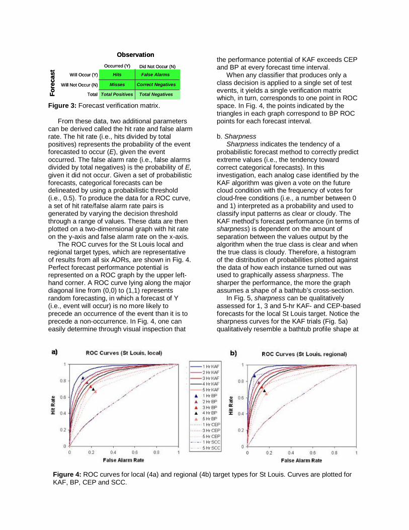
Figure 3: Forecast verification matrix. From these data, two additional parameters can be derived called the hit rate and false alarm rate. The hit rate (i.e., hits divided by total positives) represents the probability of the event forecasted to occur (E), given the event occurred. The false alarm rate (i.e., false alarms divided by total negatives) is the probability of E, given it did not occur. Given a set of probabilistic forecasts, categorical forecasts can be delineated by using a probabilistic threshold (i.e., 0.5). To produce the data for a ROC curve, a set of hit rate/false alarm rate pairs is generated by varying the decision threshold through a range of values. These data are then plotted on a two-dimensional graph with hit rate on the y-axis and false alarm rate on the x-axis. The ROC curves for the St Louis local and regional target types, which are representative of results from all six AORs, are shown in Fig. 4. Perfect forecast performance potential is represented on a ROC graph by the upper left-hand corner. A ROC curve lying along the major diagonal line from (0,0) to (1,1) represents random forecasting, in which a forecast of Y (i.e., event will occur) is no more likely to precede an occurrence of the event than it is to precede a non-occurrence. In Fig. 4, one can easily determine through visual inspection that

the performance potential of KAF exceeds CEP and BP at every forecast time interval. When any classifier that produces only a class decision is applied to a single set of test events, it yields a single verification matrix which, in turn, corresponds to one point in ROC space. In Fig. 4, the points indicated by the triangles in each graph correspond to BP ROC points for each forecast interval. b. Sharpness Sharpness indicates the tendency of a probabilistic forecast method to correctly predict extreme values (i.e., the tendency toward correct categorical forecasts). In this investigation, each analog case identified by the KAF algorithm was given a vote on the future cloud condition with the frequency of votes for cloud-free conditions (i.e., a number between 0 and 1) interpreted as a probability and used to classify input patterns as clear or cloudy. The KAF method’s forecast performance (in terms of sharpness) is dependent on the amount of separation between the values output by the algorithm when the true class is clear and when the true class is cloudy. Therefore, a histogram of the distribution of probabilities plotted against the data of how each instance turned out was used to graphically assess sharpness. The sharper the performance, the more the graph assumes a shape of a bathtub’s cross-section.

In Fig. 5, sharpness can be qualitatively assessed for 1, 3 and 5-hr KAF- and CEP-based forecasts for the local St Louis target. Notice the sharpness curves for the KAF trials (Fig. 5a) qualitatively resemble a bathtub profile shape at

observed noobserved yes

correct negativesmisses

false alarmshits

Fore

cast

Total NegativesTotal PositivesTotal

Correct NegativesMisses

False AlarmsHits

Occurred (Y)

Observation

Did Not Occur (N)

Will Occur (Y)

Will Not Occur (N)

observed noobserved yes

correct negativesmisses

false alarmshits

Fore

cast

Total NegativesTotal PositivesTotal

Correct NegativesMisses

False AlarmsHits

Occurred (Y)

Observation

Did Not Occur (N)

Will Occur (Y)

Will Not Occur (N)

Figure 4: ROC curves for local (4a) and regional (4b) target types for St Louis. Curves are plotted for KAF, BP, CEP and SCC.

Figure 5. 1-, 3-, and 5-hr Sharpness curves for the local target type in the St Louis AOR. a) KAF sharpness curves. b) CEP sharpness curves. all hours while the “floor” of the tub is elevated with each passing forecast hour. The CEP sharpness curves (Fig. 5b) contain multiple peaks and hence don’t qualitatively assume a bathtub profile shape (i.e., they are relatively less sharp than the KAF curves). These data are representative of the performance at all forecast intervals for both AORs and target types. c. Accuracy Accuracy for this investigation was taken as the percent correct match (PCM) defined as the percent of total forecasts (i.e., total forecasts = hits + correct negatives + misses + false alarms)

that turned out to be correct (i.e., either a hit or a correct negative). It is derived from the parameters in the verification matrix (Fig. 3) as (hits + correct negatives)/(total forecasts). Determination of PCM requires choosing a probabilistic decision threshold at which the forecast is made. Given a forecast sky condition probability provided by the KAF algorithm in this investigation, we used a threshold of 0.5 to transform each probabilistic forecast into a categorical forecast of cloudy or clear. This threshold minimizes the probability of error, P(error) which is equal to 1 – P(correct forecast). PCM is the maximum likelihood estimator for P(correct forecast). The average accuracy of KAF, CEP, BP, and SCC across all AORs at each forecast interval for both target types is shown in Fig. 6. KAF’s accuracy, on average, is greater than the benchmark methods at all forecast intervals with the advantage of KAF increasing with time. The accuracy of CEP and BP was essentially equal, on average, at all forecast intervals. d. EBC One advantage of probabilistic forecast methods over deterministic methods is that they allow predictions to be ranked, expected costs minimized, and value maximized. In a situation where the decision cost of a false alarm is high (in terms of resources or risk), actions that cause expenditure of resources or unpalatable exposure to risk should be taken only when there is high confidence in the event occurring. Conversely, if the cost of a miss, rather than of a false alarm, is prohibitively high, the number of actions should be increased by relaxing the required confidence level (i.e., probability threshold) that prompts a decision to act. So, each user of a forecast system has a specific or cost-loss operating structure with a uniquely optimal balance of hits and false alarms. In this investigation, EBC (a value metric) was used to assess the performance of each forecast method in operating paradigms with different cost-value ratios. The basic premise of the cost-loss problem is that a decision maker is faced with the uncertain prospect of a weather event (E). As discussed by Murphy and Ehrendorfer (1987), the prototype cost-loss scenario is a problem involving two possible decisions to act or not and the two weather events (E), described previously. Let f = 0 represent a categorical forecast of clear sky condition and f = 1 a cloudy sky condition forecast. The decision maker

incurs a cost c (> 0) if action is taken and (E = 1), a cost equivalent to (c – v) if action is taken and E = 0, and a cost equivalent to (v – c) if no action is taken and (E = 0). Here, v (≥ 0) is the additional value of taking the action when (E = 0) (not including the cost of the action). Note that if (v > c), the cost would turn out to be negative meaning a “profit” is realized. For this investigation, this problem was considered in terms of an expected best cost (EBC) expressed in terms of the value-cost ratio (α = v/c). If (E = 1), then (v = 0). The decision maker was assumed to take action or not in order to maximize “profit” (i.e., minimize cost) such that α > 1. The use of a specific probabilistic threshold to transform the probabilistic forecast output by the KAF algorithm into a categorical forecast will generate the following probabilities: P00 = P(f = 0 | E = 0), P10 = P(f = 1 | E = 0), P01 = P(f = 0 | E = 1), P11 = P(f = 1 | E = 1). The training data can also be used to generate the a priori probabilities P0 = P(E = 0), and P1 = P(E=1). It can be shown that the EBC, or max net “profit” per action taken or not taken based on a forecast method, on average, is equivalent to:

101010)1(2)1( PPPPcEBC

With c = -100 monetary units, the variation in average EBC across all AORs for KAF, CEP, SCC, and BP with increasing value-cost ratio (α) is shown in Fig. 7 for both target types. Similarly, Fig. 8 depicts the variation in EBC with increasing forecast interval. KAF is the most profitable forecast method (on average) across the six AORS, for all values of α from 2 to 5 (Fig. 7), and all forecast intervals (Fig. 8). The advantage of KAF over CEP increases with increasing α and decreases slightly with increasing forecast interval. The advantage of KAF over BP increases both with increasing α, and increasing forecast interval. The profit gap between KAF and SCC narrows with increasing α (Fig. 7) for both target types. Taken out to α = 15 (not shown), EBC for CEP and SCC are essentially equivalent (for α ≥ ~ 10), but remain less profitable than KAF. e. Reliability Reliability is equivalent to bias and answers the question of how well the predicted probabilities of an event correspond to their observed frequencies. It complements ROC analysis and the EBC metric. To calculate reliability, probabilities output from the KAF algorithm were rounded to the nearest tenth and binned. All cases falling in each bin were examined to determine how many had an outcome of clear (E = 0). The observed

Figure 6: Average accuracy for the local (6a) and regional (6b) target types across all AORs for KAF, BP, CEP and SCC.

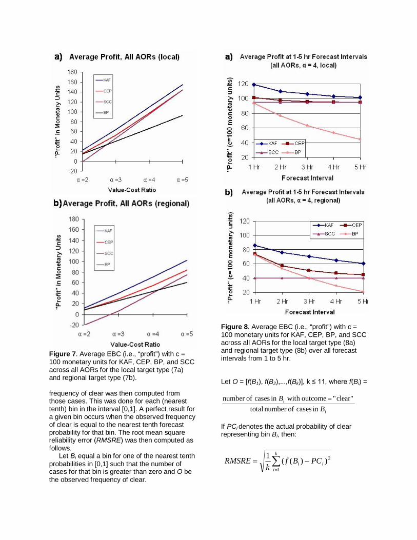
Figure 7. Average EBC (i.e., “profit”) with c = 100 monetary units for KAF, CEP, BP, and SCC across all AORs for the local target type (7a) and regional target type (7b). frequency of clear was then computed from those cases. This was done for each (nearest tenth) bin in the interval [0,1]. A perfect result for a given bin occurs when the observed frequency of clear is equal to the nearest tenth forecast probability for that bin. The root mean square reliability error (RMSRE) was then computed as follows. Let Bi equal a bin for one of the nearest tenth probabilities in [0,1] such that the number of cases for that bin is greater than zero and O be the observed frequency of clear.

Figure 8. Average EBC (i.e., “profit”) with c = 100 monetary units for KAF, CEP, BP, and SCC across all AORs for the local target type (8a) and regional target type (8b) over all forecast intervals from 1 to 5 hr. Let O = [f(B1), f(B2),...,f(Bk)], k ≤ 11, where f(Bi) =

i

i

BB

in cases ofnumber total clear"" outcome with in cases ofnumber

If PCi denotes the actual probability of clear representing bin Bi, then:

2

1))((1 ii

k

iPCBf

kRMSRE

Reliability for the KAF and CEP methods is shown in Fig. 9 for the St Louis local and regional targets at all five forecast intervals by plotting the observed frequency of clear versus the forecast probability of clear (nearest tenth), together with the value computed for the average RMSRE. Theoretical, perfect reliability is shown by the emboldened line that extends from the origin (0,0) to the point (1,1) in the upper right-hand corner of the chart. Note that the performance of KAF is highly reliable over the range of forecast probabilities. These results are representative of all AORs. 7. DISCUSSION The findings from this investigation demonstrate that an analog forecast scheme based on a k-nn algorithm can successfully generate high quality, very short-range, probabilistic, sky condition forecasts for local and regional targets in six weather regimes. Based on ROC analysis, accuracy, EBC, sharpness, and reliability, the KAF algorithm outperformed BP, CEP and SCC forecasts at all intervals for both target types. For a global application, a CHANCES-class (Reinke et al. 2003), high spatial/temporal resolution satellite imagery, multi-year time series constructed from low-earth orbiting and geostationary weather satellites would be required. Additionally, imagery from future LEO

satellites such as NPOESS would be needed to initialize analog queries for some geographic regions (e.g., polar). CEP cloud forecasts, based on past satellite records, performed very well and would be worthy of use if a forecast based on a predictive scheme such as KAF is not available. 8. ACKNOWLEDGEMENTS This work was sponsored by the NPOESS program under contract number DG133E07CQ0005. We extend our appreciation to Ken Knapp for his assistance with developing a GVAR reader. 9. REFERENCES Aha, D. W., 1998: Feature weighting for lazy learning algorithms. Feature Extraction. Construction, and Selection: A Data Mining Perspective, H. Liu and H. Motoda, eds., Kluwer, 13-29. [Available for download at http://www.aic.nrl.navy.mil/papers/1998/AIC-98-003.ps] Bankert, R. L, and M. Hadjimichael, 2007: Data mining numerical model output for single-station cloud-ceiling forecast algorithms. Wea. Forecasting, 22, 1123-1131.

Figure 9: Reliability for St Louis local and regional target types for KAF (9a) and CEP (9b). Perfect reliability is indicated by emboldened black line extending from the origin (0,0) to the upper right-hand corner (1,1). RMSRE is average root mean squared reliability error for all forecast intervals.

Bellman, R. E., 1961: Adaptive control processes. Princeton University Press. 273 pp. Beyer, K., J. Goldstein, R. Ramakrishnan, and U. Shaft, 1999: “When Is `Nearest Neighbor' Meaningful?”, Proc. 7th International Conference on Database Theory, Jerusalem, Israel, Assoc. Comp. Machinery Spec. Int. Group on Man. of Data, 217-235. Black, T. L., 1994: The new NMC mesoscale Eta Model: Description and forecast examples. Wea. Forecasting, 9, 265-278. Breiman, L., 2001: Random forests. Machine Learning, 45, 5-32. Breiman, L., J. H. Friedman, R. A. Olshen, and C. J. Stone, 1998: Classification and regression trees. Chapman & Hall, 368 pp. Blanchard, D. O., and R. E. Lopez, 1985: Spatial patterns of convection in south Florida. Mon. Wea. Rev., 113, 1282-1299. Combs, C.L., W. Blier, W. Strach, M., DeMaria, 2004: Exploring the timing of fog formation and dissipation over San Francisco Bay area using satellite cloud composites. Preprints, 13th Conf. Satellite Meteorology and Oceanography, Norfolk, VA, Amer. Meteor. Soc. Connell, B. H., K. Gould, and J. F. W. Purdom, 2001: High-resolution GOES-8 visible and infrared cloud frequency composites over northern Florida during the summers 1996-1999. Wea. Forecasting, 16, 713-724. Enger, I., L. J. Reed, and J. E. MacMonegle, 1962: An evaluation of 2-7-hr aviation terminal-forecasting techniques. Interim Report Technical Publication 20 prepared for the Federal Aviation Agency, Systems Research and Development Service by the Travelers Research Center Inc., 43 pp. Fukunaga, K., 1990: Introduction to Statistical Pattern Recognition. Academic Press, 592 pp. Girodo, M., R. W. Mueller, and D. Heinemann, 2006: Influence of three-dimensional cloud effects on satellite derived solar irradiance estimation—first approaches to improve the Heliosat methods. Solar Energy, 80, 1145-1159.

Hall, T. J., D. L. Reinke, and T. H. Vonder Haar, 1998: Forecasting applications of high-resolution satellite cloud composite climatologies. Wea. Forecasting, 13, 16-23. Hall, T. J., R. N. Thessin, G. J. Bloy and C. N. Mutchler, 2009: Analog sky condition forecasting based on a k-nn algorithm. Submitted to Wea. Forecasting. Hall, T. J., C. N. Mutchler, and S. K. Gaffney, 2010: Operational concept for observation-based forecasting of clear sky condition. 6th Annual Symp. of Future NPOESS and GOES-R, Atlanta, GA, Amer. Meteor. Soc. Hansen, B., 2007: A fuzzy logic-based analog forecasting system for ceiling and visibility. Wea. Forecasting, 22, 1319-1330. Harvey, L. O. Jr., K. R. Hammond, C. M. Lusk, and E. F. Mross, 1992: The application of signal detection theory to weather forecasting behavior. Mon. Wea. Rev., 120, 863-883. Jedlovec, G. J., S. L. Haines, and F. J. LaFontaine, 2008: Spatial and temporal varying thresholds for cloud detection in GOES imagery. IEEE Trans. Geosci. Rem. Sens., 46, 1-13. Johns, M. V. 1961: An empirical Bayes approach to nonparametric two-way classification. Studies in item analysis and prediction, H. Soloman, ed., Stanford University Press, 221-232. Kelly, F. P., 1988: Spatial and temporal short range total cloud cover estimation by metric analysis of composite imagery, Ph.D. dissertation, Department of Atmospheric Science, Colorado State University, Fort Collins, CO, 152 pp. Mason, S. J., and N. E. Graham, 2002: Areas beneath the relative operating characteristic (ROC) and relative operating levels (ROL) curves: Statistical significance and interpretation. Q. J. R. Meteorol. Soc., 128, 2145-2166. Mason, I., 1982: A model for assessment of weather forecasts. Aus. Met. Mag., 30, 291-303.

Murphy, A. H., and M. Ehrendorfer, 1987: On the relationship between the accuracy and value of forecasts in the cost-loss ratio situation. Wea. Forecasting, 2, 243-251. Norquist, D. C., 1999: Cloud predictions diagnosed from global weather model forecasts. Mon. Wea. Rev., 128, 3528-3555. Quinlan, J. R., 1986: Induction of decision trees. Machine Learning, 1, 81-106. Reinke, D. L., C. L. Combs, S. Q. Kidder and T. H. Vonder Haar, 1992: Satellite cloud composite climatologies: A new high-resolution tool in atmospheric research and forecasting. Bull. Amer. Meteor. Soc., 73, 278-285. Reinke, D. L., and J. M. Forsythe, 2003: A cloud hangs over Iraq. CIRA Newsletter, Colorado State University, 19, 3-7. Reinke, D. L., J. M. Forsythe, J. A. Kankiewicz, K. R. Dean, C. L. Combs, and T. H. Vonder Haar, 2003: Development and applications of regional cloud products from the CHANCES global cloud database. 12th Conf. on Satellite Meteorology and Oceanography, Long Beach, CA, Amer. Meteor. Soc. Vislocky, R. L., and J. M. Fritsch, 1997: An automated, observation-based system for short-term prediction of ceiling and visibility. Wea. Forecasting, 12, 31-43. Wettschereck, D., 1994: A study of distance-based machine learning algorithms. Doctoral dissertation, Oregon State University, Department of Computer Science. Witten, I. H., and E. Frank, 2005: Data Mining: Practical Machine Learning Tools and Techniques. Morgan Kaufmann, 560 pp.