18/6/2008 andrew beddall tr-atlas gaziantep grid workshop june 19-21 2008 1 introduction to data...
Post on 20-Dec-2015
221 views
TRANSCRIPT

18/6/2008 Andrew Beddall TR-ATLAS Gaziantep Grid Workshop June 19-21 2008 1
Introduction to Data Analysis1. An Apple Collider Experiment
(Toy Monte Carlo Simulation)
2. A couple of analysis examples from ALEPH at the LEP collider (data taking 1989 to 1995)
3. What does it look like at ATLAS? (data taking 2008[?] ...)
Dr Andrew Beddall, University of Gaziantep

Introduction to Data Analysis
1. An Apple Collider Experiment(Toy Monte Carlo Simulation)
18/6/2008 2Andrew Beddall TR-ATLAS Gaziantep Grid Workshop June 19-21 2008

Counting ExperimentsExperimental High Energy Physics is about counting (frequency) experiments.
Example: An apple-apple collider.
If we perform n apple-apple collisions (at high energy, of course)and observe m cherries amongst the mush, then we can say therate (or probability) R(apple,apple cherry + mush) m/n Or more specifically R = (m/n) ± (m /n) (counting error)*
But what is the relationship between probability and counting?
*assuming m is > 10 or so.
18/6/2008 Andrew Beddall TR-ATLAS Gaziantep Grid Workshop June 19-21 2008 3
AfterBefore

18/6/2008 Andrew Beddall TR-ATLAS Gaziantep Grid Workshop June 19-21 2008 4
You can find anything at Wikipedia!http://en.wikipedia.org/wiki/Frequentist

18/6/2008 5Andrew Beddall TR-ATLAS Gaziantep Grid Workshop June 19-21 2008
Counting (n = n):Entries 436 ± 20.9 cherries Log likelihood fit:L.L. fit = 27.250 ± 1.305 x16 bins 436.0 ± 20.9 cherries
Cherry rate calculation:C = 436.0 ± 20.9 cherries 106 collisions
(4.360 ± 0.209) x 10-4
Cherries per collision
Experiment 1: Say, in nature R(apple,apple cherry + mush) = 4 x 10⁻⁴
Perform one million apple-apple collisions, count the number of cherries.
χ2 fitting underestimates in the presence of low statistics (the dash line); so we won’t use that here.
x

18/6/2008 Andrew Beddall TR-ATLAS Gaziantep Grid Workshop June 19-21 2008 619/06/2008 6Andrew Beddall TR-ATLAS Gaziantep Grid Workshop June 19-21 2008
Counting (n = n):Entries 374 ± 19.3 cherries Log likelihood fit:L.L. fit = 23.375 ± 1.2086 x16 bins 374.0 ± 19.3 cherries
Cherry rate calculation:C = 374.0 ± 19.3 cherries 106 collisions
(3.740 ± 0.193) x 10-4
Cherries per collision
Experiment 2: Repeat the experiment.
x

18/6/2008 Andrew Beddall TR-ATLAS Gaziantep Grid Workshop June 19-21 2008 719/06/2008 Andrew Beddall TR-ATLAS Gaziantep Grid Workshop June 19-21 2008 719/06/2008 7Andrew Beddall TR-ATLAS Gaziantep Grid Workshop June 19-21 2008
Counting (n = n):Entries 414 ± 20.3 cherries Log likelihood fit:L.L. fit = 25.875 ± 1.2716 x16 bins 414.0 ± 20.3 cherries
Cherry rate calculation:C = 414.0 ± 20.3 cherries 106 collisions
(4.140 ± 0.203) x 10-4
Cherries per collision
Experiment 3: Repeat the experiment.
x

18/6/2008 Andrew Beddall TR-ATLAS Gaziantep Grid Workshop June 19-21 2008 8
Summary:
In nature R(apple,apple cherry + mush) = 4 x 10⁻⁴
Exp. 1: C = (4.36 ± 0.21) x 10-4 (1.7 )Exp. 2: C = (3.74 ± 0.19) x 10-4 (1.4 )Exp. 3: C = (4.14 ± 0.20) x 10-4 (0.7 )
But is “n = n” true, and is actually meaningful?
Number of standard deviations from the true rate.

18/6/2008 Andrew Beddall TR-ATLAS Gaziantep Grid Workshop June 19-21 2008 9
The normal (Gaussian) distribution.The numbers of ’s defines confidence intervals.
Exp. 1: R = (4.36 ± 0.21) x 10-4 R = (4.36 ± 0.42) x 10-4
Exp. 2: R = (3.74 ± 0.19) x 10-4 R = (3.74 ± 0.38) x 10-4
Exp. 3: R = (4.14 ± 0.20) x 10-4 R = (4.14 ± 0.40) x 10-4
1 68% confidence 2 ’s 95% confidence
We expect that if we repeat the experiment many times, then 68% (95%) of our results would be within 1 (2 ) of the true rate.
true rate 4 x 10⁻⁴
SO LET’S DO IT! ...
Here, is about 0.2 (the experimental accuracy)

18/6/2008 Andrew Beddall TR-ATLAS Gaziantep Grid Workshop June 19-21 2008 10
Each entry in the histogram is the result of an experiment to determine R.
We have a perfect fit to a Gaussian function!
The value of is 0.2 That’s the same as the accuracy of our individual results. This explains what is .
Furthermore, is the standard deviation of the distribution, the standard error SE = /10000 = 0.002 x 10⁻⁴ is a measure of the uncertainty in the mean.
So we can write the overall result as: R = (3.995 ± 0.002) x 10-4 fitted R = (3.999 ± 0.002) x 10-4 calculated[two more decimal places of accuracy]

Summary so far• I did not fiddle the results in any way – honest!
• This toy Monte Carlo has demonstrated the basic concept of n errors and how they are used to obtain estimates of accuracy in counting experiments.
• The experimental accuracy scales as 1/ n .but if statistics are large then systemic errors dominate.
• χ2 fits tend to underestimate when statistics are small.
• If stats are very small (discoveries) probability estimation is very different(see the endless debates in the statistic forums/conferences).
• What if our signal is mixed with background?See next .....
18/6/2008 Andrew Beddall TR-ATLAS Gaziantep Grid Workshop June 19-21 2008 11

18/6/2008 Andrew Beddall TR-ATLAS Gaziantep Grid Workshop June 19-21 2008 12
New situation: R(apple,apple cherry + mush) = 4 x 10⁻⁴
But the some of the mush is selected with the signalPerform one million apple-apple collisions, count the number of cherries.
The background mixes with the signal, the bin-to-bin variations are increased in the signal region and we don’t know which is signal and which is background!
This time we must use fitting, to estimate the background + signal and subtract the background estimate from the signal estimate.
The fitting function is
f(x) = p1 + p2 for 0.42 < x < 0.58 f(x) = p2 elsewhere p1 x 16 bins = signal count.
p1 and p2 are free parameters in the fit.
x

18/6/2008 Andrew Beddall TR-ATLAS Gaziantep Grid Workshop June 19-21 2008 13
Experiment 1: (same signal as in the previous Exp 1)Perform one million apple-apple collisions, count the number of cherries.
Entries 2962 cherries+mush
Log likelihood fit:p1 = 27.842 ± 1.894x16 bins 445.5 ± 30.3 cherries
(4.455 ± 0.303) x 10-4
Cherries per collision
Check:p2 = 25.170 ± 0.546x100 bins 2517.0 ± 54.6 mush
445.5+2517.0 = 2962.5 entries, ok.x

18/6/2008 Andrew Beddall TR-ATLAS Gaziantep Grid Workshop June 19-21 2008 1419/06/2008 Andrew Beddall TR-ATLAS Gaziantep Grid Workshop June 19-21 2008 14
Experiment 2: (same signal as in the previous Exp 2)Repeat the experiment .
Entries 2862 cherries+mush
Log likelihood fit:p1 = 25.384 ± 1.841x16 bins 406.1 ± 29.5 cherries
(4.061 ± 0.295) x 10-4
Cherries per collision
Check:p2 = 24.562 ± 0.539x100 bins 2456.2 ± 53.9 mush
406.1+2456.2 = 2862.3 entries, ok.x

18/6/2008 Andrew Beddall TR-ATLAS Gaziantep Grid Workshop June 19-21 2008 1519/06/2008 Andrew Beddall TR-ATLAS Gaziantep Grid Workshop June 19-21 2008 1519/06/2008 Andrew Beddall TR-ATLAS Gaziantep Grid Workshop June 19-21 2008 15
Experiment 3: (same signal as in the previous Exp 3)Repeat the experiment.
Entries 2961 cherries+mush
Log likelihood fit:p1 = 25.095 ± 1.857x16 bins 401.5 ± 29.7 cherries
(4.015 ± 0.297) x 10-4
Cherries per collision
Check:p2 = 25.599 ± 0.550x100 bins 2559.9 ± 55.0 mush
401.5+2559.9 = 2961.4 entries, ok.x

18/6/2008 Andrew Beddall TR-ATLAS Gaziantep Grid Workshop June 19-21 2008 1619/06/2008 Andrew Beddall TR-ATLAS Gaziantep Grid Workshop June 19-21 2008 16
Summary and Discussion: the analysis repeated with background
In nature R(apple,apple cherry + mush) = 4 x 10⁻⁴
Exp. 1: C = (4.46 ± 0.30) x 10-4 (1.5 )Exp. 2: C = (4.06 ± 0.30) x 10-4 (0.2 )Exp. 3: C = (4.02 ± 0.30) x 10-4 (0.05 ) chance!
Number of standard deviations from the true rate.
The effect of background has been to increased from 0.20 to 0.30
Let’s repeat the experiment 10,000 times and look at the distribution of R values. .....
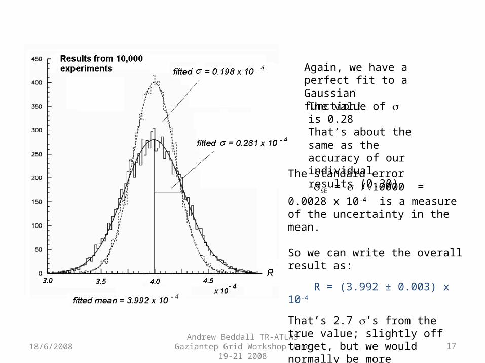
18/6/2008 Andrew Beddall TR-ATLAS Gaziantep Grid Workshop June 19-21 2008 17
Again, we have a perfect fit to a Gaussian function!
The value of is 0.28 That’s about the same as the accuracy of our individual results (0.30).
The standard error SE = /10000 = 0.0028 x 10⁻⁴ is a measure of the uncertainty in the mean.
So we can write the overall result as:
R = (3.992 ± 0.003) x 10-4
That’s 2.7 ’s from the true value; slightly off target, but we would normally be more conservative than this;fitting can be tricky a tricky business.

18/6/2008 Andrew Beddall TR-ATLAS Gaziantep Grid Workshop June 19-21 2008 18
Note that the background amplitude is the about the same as the signal amplitude.
As n then, because we have twice the number of counts, we expect to increase by a factor of 2.
For signal only data = 0.198 x 10⁻⁴
With signal + background we expect = 0.198 x 10-4 x 2 = 0.280 x 10⁻⁴
We actually see 0.281 x 10⁻⁴ Same!
Conclusion:In our counting experiment, the statistics behave as we expect.
x

18/6/2008 Andrew Beddall TR-ATLAS Gaziantep Grid Workshop June 19-21 2008 19
An Apple Collider Experiment (Toy Monte Carlo Simulation)
SUMMARY * This was a long winded way to say: “We observe n events with an uncertainty n”, but we proved it! (for this experiment at least).
* Background degrades statistical accuracy (see signal significance). Caution: * If we have background we usually rely on fitting (which is not to be trusted 100%).
* χ2 fits tend to underestimate when statistics are small.
* If stats are very small (discoveries) probability estimation is very different. (use Poisson statistics).
* Experiments are much more complex than this toy simulation (see next section).
* In reality R(apple,apple cherry + mush) <<< 4 x 10⁻⁴ !

Additional Notes – Signal Significance, Q
We select S signal events with and uncertainty (S+B)where B is the number of selected background events.
The ratio Q = S/ (S+B) is called signal significance;sometimes written as S/ B (what if B 0 ?!)
It is desirable to maximise Q (to minimise the relative error in a measurement).This is usually done by optimising cuts such that background is reduced withminimal reduction in signal.
“Optimal” is often not easy to quantify, especially where selection cuts aremulti-dimensional.
A quantitative method for cut optimisation is to maximise the product:
Signal Purity x Signal Efficiency
18/6/2008 Andrew Beddall TR-ATLAS Gaziantep Grid Workshop June 19-21 2008 20

18/6/2008 Andrew Beddall TR-ATLAS Gaziantep Grid Workshop June 19-21 2008 21
Selection of signalwith more or less background
Signal
Signal

18/6/2008 Andrew Beddall TR-ATLAS Gaziantep Grid Workshop June 19-21 2008 22
Introduction to Data Analysis
2. A couple of analysis examples from ALEPH at the LEP collider
(data taking 1989 to 1995)
18/6/2008 Andrew Beddall TR-ATLAS Gaziantep Grid Workshop June 19-21 2008 23
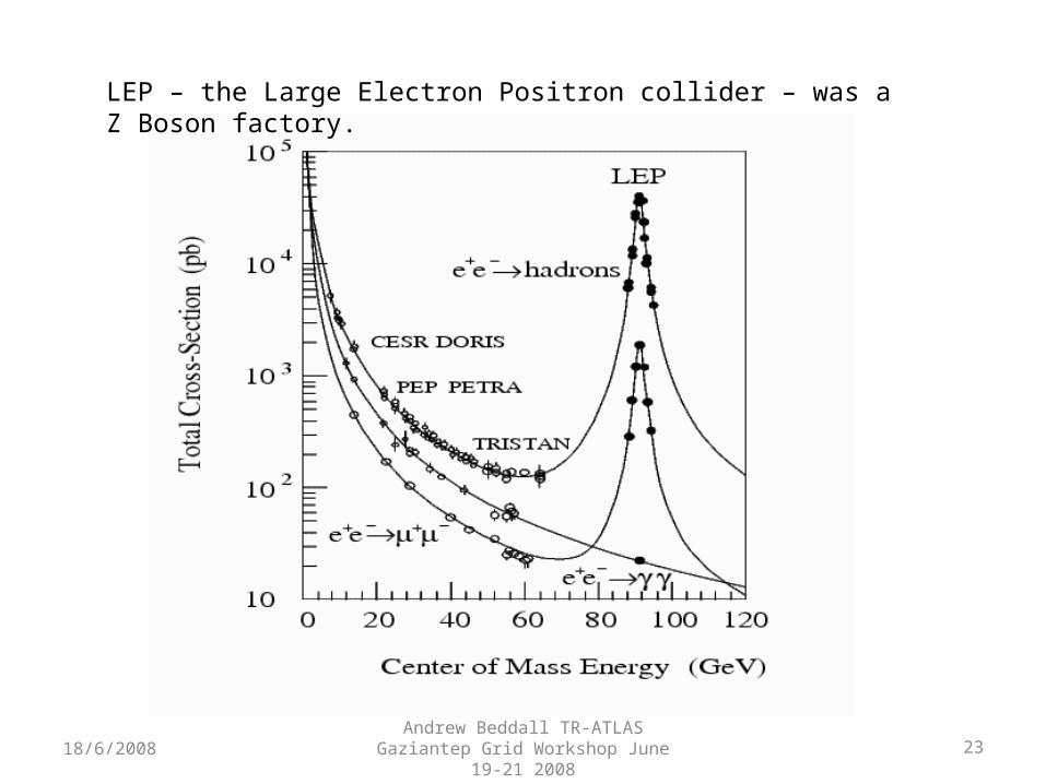
LEP – the Large Electron Positron collider – was a Z Boson factory.

18/6/2008 Andrew Beddall TR-ATLAS Gaziantep Grid Workshop June 19-21 2008 24

18/6/2008 Andrew Beddall TR-ATLAS Gaziantep Grid Workshop June 19-21 2008 25
18/6/2008 Andrew Beddall TR-ATLAS Gaziantep Grid Workshop June 19-21 2008 26

18/6/2008 Andrew Beddall TR-ATLAS Gaziantep Grid Workshop June 19-21 2008 27

18/6/2008 Andrew Beddall TR-ATLAS Gaziantep Grid Workshop June 19-21 2008 28

18/6/2008 Andrew Beddall TR-ATLAS Gaziantep Grid Workshop June 19-21 2008 29

18/6/2008 Andrew Beddall TR-ATLAS Gaziantep Grid Workshop June 19-21 2008 30

18/6/2008 Andrew Beddall TR-ATLAS Gaziantep Grid Workshop June 19-21 2008 31

18/6/2008 Andrew Beddall TR-ATLAS Gaziantep Grid Workshop June 19-21 2008 32

Example 1
A simple analysis: BR(Z + -)
Extracts from the presentation given by Bob Jacobsen
“From Raw Data to Physics”CERN Summer School 2006
For the full presentation (on video), seehttp://agenda.cern.ch/fullAgenda.php?ida=a062776
18/6/2008 Andrew Beddall TR-ATLAS Gaziantep Grid Workshop June 19-21 2008 33

18/6/2008 Andrew Beddall TR-ATLAS Gaziantep Grid Workshop June 19-21 2008 34
Measure:
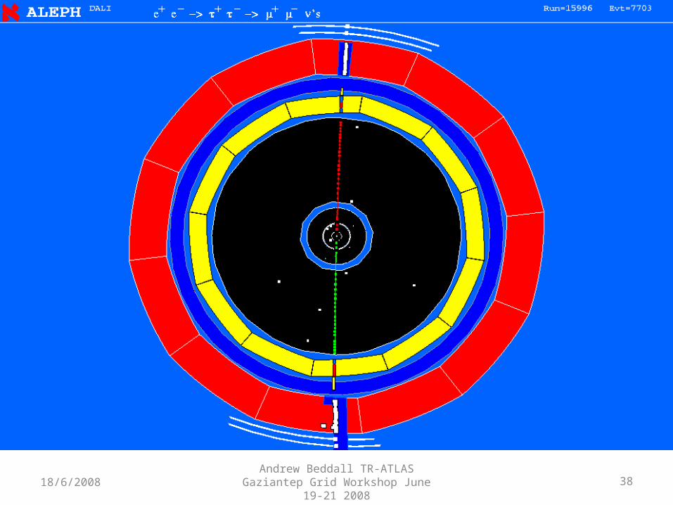
Take a sample of events, and count those with a final state.
Look for two tracks, approximately back-to-back with the expected |p|Empirically, other kinds of events have more tracks
Look for muon hits in outer layersMuons are very penetrating, travel through entire detector
Look for only small energy in calorimetersElectrons will deposit most of their energy early in the calorimeter,muons deposit little energy.
BR Z 0 Number of events
Total number of events
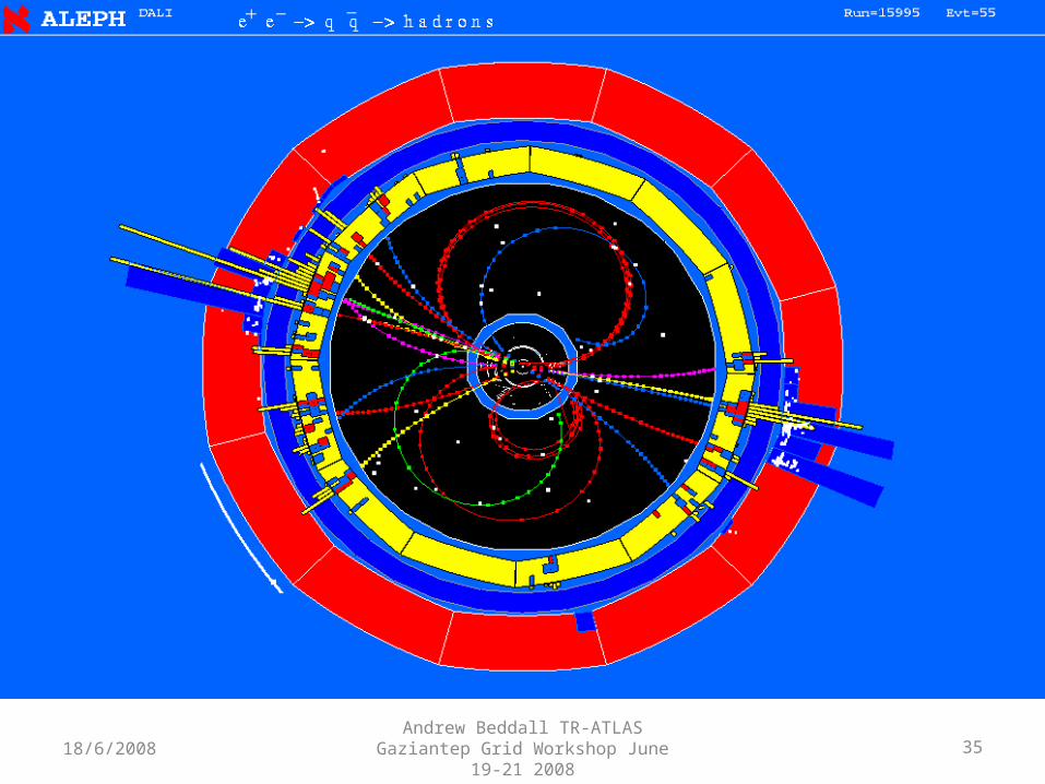
18/6/2008 Andrew Beddall TR-ATLAS Gaziantep Grid Workshop June 19-21 2008 35

18/6/2008 Andrew Beddall TR-ATLAS Gaziantep Grid Workshop June 19-21 2008 36

18/6/2008 Andrew Beddall TR-ATLAS Gaziantep Grid Workshop June 19-21 2008 37
18/6/2008 Andrew Beddall TR-ATLAS Gaziantep Grid Workshop June 19-21 2008 38

18/6/2008 Andrew Beddall TR-ATLAS Gaziantep Grid Workshop June 19-21 2008 39

18/6/2008 Andrew Beddall TR-ATLAS Gaziantep Grid Workshop June 19-21 2008 40

18/6/2008 Andrew Beddall TR-ATLAS Gaziantep Grid Workshop June 19-21 2008 41

18/6/2008 Andrew Beddall TR-ATLAS Gaziantep Grid Workshop June 19-21 2008 42

18/6/2008 Andrew Beddall TR-ATLAS Gaziantep Grid Workshop June 19-21 2008 43

18/6/2008 Andrew Beddall TR-ATLAS Gaziantep Grid Workshop June 19-21 2008 44
And so on ....... For ~ a million events

18/6/2008 Andrew Beddall TR-ATLAS Gaziantep Grid Workshop June 19-21 2008 45
We see, for example, 26400 Z + - events in a total of 1,000,000 events.
The result, including statistical uncertainty is
BR( Z + - ) = N / Ntotal ± N/ Ntotal
= 0.026400 ± 0.000162
But we don’t see all events (some are lost own the beam pipe) and so we need to apply an efficiency correction factor of, for example 1.250 ± 0.004
The final result is:
BR( Z + - ) = 0.0330 ± 0.0002 ± 0.0001
0.026400 x 1.25 0.0330 x 0.004/1.250=0.0330 x 0.32% 0.000162 x 1.25
Statistical error Systematic error

18/6/2008 Andrew Beddall TR-ATLAS Gaziantep Grid Workshop June 19-21 2008 46
Example 2
± meson production in Z decays
We wish to measure the production rate of the ±
(average number per hadronic Z decay), and themomentum spectra.
test of hadronisation models.
http://durpdg.dur.ac.uk/hepdata/online/rsig/index.htmlAn up-to-date archive of data on hadronic cross sectionmeasurements in e+e- interactions.

18/6/2008 Andrew Beddall TR-ATLAS Gaziantep Grid Workshop June 19-21 2008 47

18/6/2008 Andrew Beddall TR-ATLAS Gaziantep Grid Workshop June 19-21 2008 48

18/6/2008 Andrew Beddall TR-ATLAS Gaziantep Grid Workshop June 19-21 2008 49

18/6/2008 Andrew Beddall TR-ATLAS Gaziantep Grid Workshop June 19-21 2008 50
This is a very problematic analysis!
• Large combinatoric background from charge particles• Huge combinatoric background from neutral pions• Very wide signal (on a large background)
also: • Reflections from other resonances• Böse Einstein correlations
both complicate the background shape
Very difficult to extract the signal!

18/6/2008 Andrew Beddall TR-ATLAS Gaziantep Grid Workshop June 19-21 2008 51
Let’s go back to the beginning and see how the analysis is done.....
18/6/2008 Andrew Beddall TR-ATLAS Gaziantep Grid Workshop June 19-21 2008 52
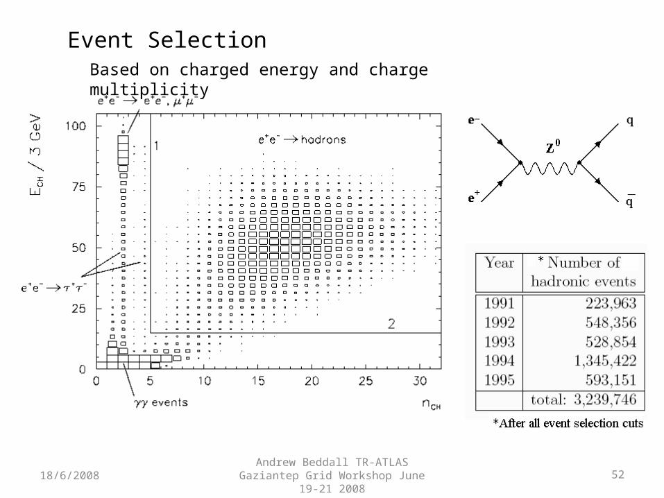
Event SelectionBased on charged energy and charge multiplicity

18/6/2008 Andrew Beddall TR-ATLAS Gaziantep Grid Workshop June 19-21 2008 53
Selecting Neutral Pions
18/6/2008 Andrew Beddall TR-ATLAS Gaziantep Grid Workshop June 19-21 2008 54
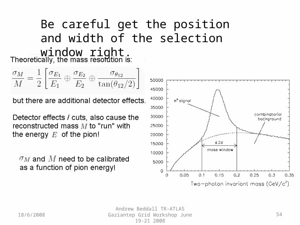
Be careful get the position and width of the selection window right.

18/6/2008 Andrew Beddall TR-ATLAS Gaziantep Grid Workshop June 19-21 2008 55
Width calibration

18/6/2008 Andrew Beddall TR-ATLAS Gaziantep Grid Workshop June 19-21 2008 56
Mass calibration

18/6/2008 Andrew Beddall TR-ATLAS Gaziantep Grid Workshop June 19-21 2008 57
Selecting Charged Pions
Mostly pions, but there is some background from electrons, muons, kaons, protons, ...
Some background can be removed by inspecting the rate of ionisation in theTPC

18/6/2008 Andrew Beddall TR-ATLAS Gaziantep Grid Workshop June 19-21 2008 58
dE/dxRate of energy loss per unit distance.

18/6/2008 Andrew Beddall TR-ATLAS Gaziantep Grid Workshop June 19-21 2008 59
Significant background is removed with a cut in the range:

18/6/2008 Andrew Beddall TR-ATLAS Gaziantep Grid Workshop June 19-21 2008 60
Also make sure tracks originate from close to the Interaction point.
Systematics!Don’t cut too tight on quantities that are not well modelled in the MC
18/6/2008 Andrew Beddall TR-ATLAS Gaziantep Grid Workshop June 19-21 2008 61
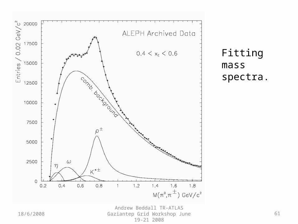
Fitting massspectra.

18/6/2008 Andrew Beddall TR-ATLAS Gaziantep Grid Workshop June 19-21 2008 62

18/6/2008 Andrew Beddall TR-ATLAS Gaziantep Grid Workshop June 19-21 2008 63
A fitted signal in one of the energy intervals.

18/6/2008 Andrew Beddall TR-ATLAS Gaziantep Grid Workshop June 19-21 2008 64
Repeat for each energy interval, and again many times to determine systematic uncertainties.

18/6/2008 Andrew Beddall TR-ATLAS Gaziantep Grid Workshop June 19-21 2008 65
Results !

18/6/2008 Andrew Beddall TR-ATLAS Gaziantep Grid Workshop June 19-21 2008 66
Total rate
18/6/2008 Andrew Beddall TR-ATLAS Gaziantep Grid Workshop June 19-21 2008 67
Introduction to Data Analysis
3. What does it look like at ATLAS? (data taking 2008[?] ...)
Extracts from the presentation given by Karl Jacobs“Physics at Hadronic Colliders”
CERN Summer School 2006
For the full presentation (on video), seehttp://agenda.cern.ch/fullAgenda.php?ida=a062814

Proton proton collisions at the LHC ~109 pp collisions / s (superposition of 23 pp-interactions per bunch crossing: pile-up)
~1600 charges particles in the detector
high particle densities high requirements for the detectors
18/6/2008 68Andrew Beddall TR-ATLAS Gaziantep Grid Workshop June 19-21 2008

What experimental signatures can be used ?
If leptons with large transverse momentum are observed: interesting physics !
Example: Higgs boson production and decay
Important signatures: • Leptons und photons • Missing transverse energy
p pqq
q
p pqq
H
WW
No leptons / photons in the initial and final state
Quark-quark scattering:
q
18/6/2008 69Andrew Beddall TR-ATLAS Gaziantep Grid Workshop June 19-21 2008

Suppression of background: Reconstruction of objects with large transverse momentum
Reconstructed tracks with pt > 25 GeV
18/6/2008 70Andrew Beddall TR-ATLAS Gaziantep Grid Workshop June 19-21 2008

The ATLAS experiment• Solenoidal magnetic field (2T) in the central region (momentum measurement)
High resolution silicon detectors: - 6 Mio. channels (80 m x 12 cm) -100 Mio. channels (50 m x 400 m) space resolution: ~ 15 m
• Energy measurement down to 1o to the beam line • Independent muon spectrometer (supercond. toroid system)
Diameter 25 mBarrel toroid length 26 mEnd-cap end-wall chamber span 46 mOverall weight 7000 Tons
18/6/2008 71Andrew Beddall TR-ATLAS Gaziantep Grid Workshop June 19-21 2008

Top Quark Production
Pair production: qq and gg-fusion Electroweak production of single top-quarks(Drell-Yan and Wg-fusion)
Run I
1.8 TeV
Run II
1.96 TeV
LHC
14 TeV
gg
90%
10%
85%
15%
5%
95%
(pb) 5 pb 7 pb 600 pb
Run I
1.8 TeV
Run II
1.96 TeV
LHC
14 TeV
(qq) (pb)
(gW) (pb)
(gb) (pb)
0.7
1.7
0.07
0.9
2.4
0.1
10
250
60
18/6/2008 72Andrew Beddall TR-ATLAS Gaziantep Grid Workshop June 19-21 2008

BR (t→Wb) ~ 100%
Both W’s decay via W ℓ (ℓ=e or ; 5%) dilepton
One W decays via Wℓ (ℓ=e or ; 30%) lepton+jets
Both W’s decay via Wqq (44%) all hadronic, not very useful
Top Quark Decays
Important experimental signatures: : - Lepton(s)
- Missing transverse momentum
- b-jet(s)
dilepton channel
lepton + jet channel

Technique used for W-mass measurement at hadron colliders:
Observables: PT(e) , PT(had)
PT() = - ( PT(e) + PT(had) ) long. component cannot
be
measured
In general the transverse mass MT is used for the determination of the W-mass
(smallest systematic uncertainty).
DØ
Z ee
,cos12 lT
lT
TW PPM
Event topology:
18/6/2008 74Andrew Beddall TR-ATLAS Gaziantep Grid Workshop June 19-21 2008

mTW (GeV)
mW= 79.8 GeV
mW= 80.3 GeV
Shape of the transverse mass distribution is sensitive to mW, the measured distribution is fitted with Monte Carlo predictions, where mW is a parameter
Main uncertainties:
result from the capability of the Monte Carlo prediction to reproduce real life:
• detector performance (energy resolution, energy scale, ….)
• physics: production model pT(W), W, ...... • backgrounds
Dominant error (today at theTevatron, and most likely also at the LHC) : Knowledge of lepton energy scale of the detector !
18/6/2008 75Andrew Beddall TR-ATLAS Gaziantep Grid Workshop June 19-21 2008

Signature of Z and W decays
Zl+l– Wl
18/6/2008 76Andrew Beddall TR-ATLAS Gaziantep Grid Workshop June 19-21 2008

How can one claim a discovery ?
Suppose a new narrow particle X is produced:
Signal significance:
B
S
N
N S
NS= number of signal eventsNB= number of background events
in peakregion
NB error on number of background events, for large numbers otherwise: use Poisson statistics
S > 5 : signal is larger than 5 times error on background. Gaussian probability that background fluctuates up by more than 5 : 10-7 discovery
peak width due to detectorresolution
m
18/6/2008 77Andrew Beddall TR-ATLAS Gaziantep Grid Workshop June 19-21 2008

Two critical parameters to maximize S
1. Detector resolution: If m increases by e.g. a factor of two, then need to enlarge peak region by a factor of two to keep the same number of signal events
NB increases by ~ 2 (assuming background flat)
S = NS/NB decreases by 2
S ~ 1 / m
“A detector with better resolution has larger probability to find a signal”
Note: only valid if H << m. If Higgs is broad detector resolution is not relevant. mH = 100 GeV → H ~0.001 GeV mH = 200 GeV → H ~ 1 GeV
mH = 600 GeV → H ~ 100 GeV H ~ mH3
2. Integrated luminosity :
NS ~ LNB ~ L
S ~ L
18/6/2008 78Andrew Beddall TR-ATLAS Gaziantep Grid Workshop June 19-21 2008
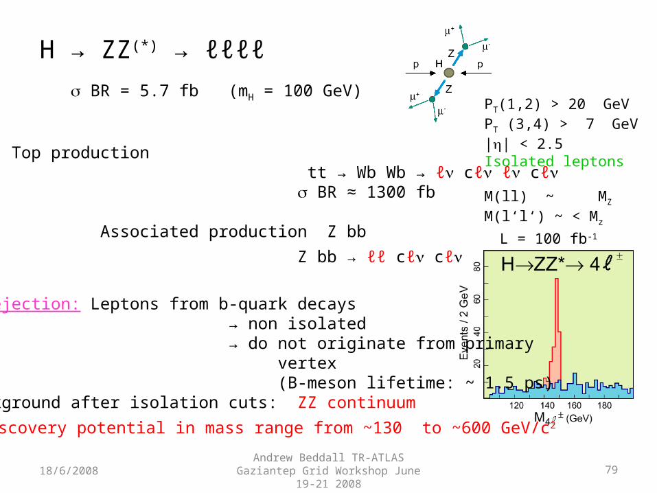
H → ZZ(*) → ℓℓℓℓSignal: BR = 5.7 fb (mH = 100 GeV)
Background: Top production tt → Wb Wb → ℓ cℓ ℓ cℓ BR ≈ 1300 fb
Associated production Z bb
Z bb → ℓℓ cℓ cℓ
Background rejection: Leptons from b-quark decays → non isolated → do not originate from primary vertex (B-meson lifetime: ~ 1.5 ps)Dominant background after isolation cuts: ZZ continuum
L = 100 fb-1
Discovery potential in mass range from ~130 to ~600 GeV/c2
PT(1,2) > 20 GeV PT (3,4) > 7 GeV|| < 2.5 Isolated leptons
M(ll) ~ MZ M(l‘l‘) ~ < Mz
18/6/2008 79Andrew Beddall TR-ATLAS Gaziantep Grid Workshop June 19-21 2008

H→ contCMS 100 fb-1
100 fb-1
ATLAS
Signal / background ~ 4% (Sensitivity in mass range 100 – 140 GeV/c2)background (dominated by events *) can be determined from side bands important: -mass resolution in the calorimeters, / jet separation
*) detailed simulations indicate that the -jet and jet-jet background can be suppressed to the level of 10-20% of the irreducible -background
Two isolated photons: PT(1) > 40 GeV PT(2) > 25 GeV || < 2.5
Mass resolution for mH = 100 GeV/c2:
ATLAS : 1.1 GeV (LAr-Pb)CMS : 0.6 GeV (crystals)
18/6/2008 80Andrew Beddall TR-ATLAS Gaziantep Grid Workshop June 19-21 2008

CERN-Fermilab Hadron Collider Physics Summer School August 9-18, 2006 “Physics Analysis”, John Womersleyhttp://vmsstreamer1.fnal.gov/VMS_Site_03/Lectures/HCPSS/060816Womersley/index.htm
CERN-Fermilab Hadron Collider Physics Summer School August 9-18, 2006 Louis Lyons - Practical Statistics for Discovery at Hadron Collidershttp://vmsstreamer1.fnal.gov/VMS_Site_03/Lectures/HCPSS/060817Lyons/index.htm
See also
2006 CERN-Fermilab HCP Summer Schoolhttp://vmsstreamer1.fnal.gov/VMS_Site_03/Lectures/HCPSS/index.htm
2007 CERN-Fermilab HCP Summer Schoolhttp://indico.cern.ch/conferenceOtherViews.py?view=cdsagenda&confId=6238
The 2008 Hadron Collider Physics Summer SchoolFermilab, August 12-22, 2008http://hcpss.web.cern.ch/hcpss/
CERN Summer School 2006“From Raw Data to Physics”, Bob Jacobsen http://agenda.cern.ch/fullAgenda.php?ida=a062776
CERN Summer School 2006“Physics at Hadronic Colliders”, Karl Jacobshttp://agenda.cern.ch/fullAgenda.php?ida=a062814
Further Viewing
18/6/2008 81Andrew Beddall TR-ATLAS Gaziantep Grid Workshop June 19-21 2008