NASA Contractor Report185676

//_ / .

7

Reference Equations of Motion forAutomatic Rendezvous and Capture

David M. HendersonTRW Systems Services Company,

Houston, Texas(TFIW Report Number 91:J431.1-182)

Inc.

Prepared forLyndon B. Johnson Space Flight Center

under contract NASg-17900

1992

(NASA-CR-185676) REFERENCE

EQUATIONS OF UOTION FOR AUTOMATIC

RENDEZVOUS A_D CAPTURE (TRW) 40 p

N93-29652

Unclas

G3/13 0176443

https://ntrs.nasa.gov/search.jsp?R=19930020463 2020-02-18T06:43:07+00:00Z

NASA Contractor Report 185676

ReferenceAutomatic

Equations ofRendezvous

Motion for

and Capture

David M. Henderson

Contract NAS9-17900

April 1992

TABLE OF CONTENTS

3.0

4.0

5.0

6.0

7.0

8.0

INTRODUCTION ...................................................... 1

TRANSLATION DYNAMICS - MOTION OF THE CENTEROF MASS .......................................................... 3

ROTATIONAL DYNAMICS - VEHICLE ANGULAR MOTIONABOUT THE CENTER OF MASS ........................................... 9

SIX DEGREES OF FREEDOM EQUATIONS OF MOTION .......................... 1 1

TRANSlaTION CONTROL PARAMETERS .................................. 1 4

ROTATION CONI"ROL PARAMETERS ....................................... 2 1

CONCLUSIONS AND RECOtV_ENDA_ ................................. 2 5

REFERENCES ...................................................... 2 6

APPENDIX A

APPENDIX B

APPENDIX C

SUGGESTED INTEGRABLE PARAMETER UST ........................... 2 7

GRAVITATIONAL ACCELERATION .................................... 2 9

PARTIAL DERIVATIVES OF THE GRAVITATIONAL ACCELERATION VECTOR ..... 3 2

iii

f

REFERENCE EQUATIONS OF MOTION FOR

AUTOMATIC RENDEZVOUS AND CAPTURE

David M. Henderson

TRW/Houston

1.0 INTRODUCTION

The analysis presented in this paper defines the reference

coordinate frames and control parameters necessary to model the

relative motion and attitude of spacecraft in close proximity with

another space system during the Automatic Rendezvous and Capture

phase of an on-orbit operation. Translation motion equations

relative to the geodesic LVLH frame are developed yielding the

Clohessy-Wiltshire differential equations of motion.

Perturbations of the gravity partial derivative matrix due to a

4x4 gravity model show the expected deviations from the Clohessy-

Wiltshire approximation. For the docking case, however, as the

relative separation distances become small, both relative

gravitational and inertial accelerations can be omitted from the

translation equations of motion.

Euler's equation for the rotational rate accelerations of a rigid

body are developed with expected torque effects indicated. The

actual torque computations are problematic and these specific

models are not developed as part of this work.

The relative docking port target position vector and the attitude

control matrix are defined based upon an arbitrary spacecraft

design. These translation and rotation control parameters could

be used to drive the error signal input to the vehicle flight

control system. Measurements for these control parameters would

become the bases for an autopilot or FCS design for a specific

spacecraft.

Cartesian analysis is used throughout the paper for the clarity

and compactness in representing component equations. The use of

Cartesian tensor notation makes the task of repeated

differentiation of transformation equations considerably easier

and more understandable. For instance, the position vector in

inertial space is given by

x = a R + X (I.I)

where aR is a transformation matrix times the vector R. Equation

I.i defines both rotation and translation in the inertial frame.

Differentiating Equation I.i for velocity is simply,

v -- a_ + V (1.2)

where

= W R + 9 (1.3)

and W is the skew-symmetry angular velocity matrix. The vector

is recognized from vector analysis [see Reference 4.0, Page 208]

as the operator,

+ -- x

dt(1.4)

However, in Equation 1.2 the inertial coordinates are preserved

and no ambiguities arise as to which coordinate system the vectors

components are represented.

2

2.0 TRANSLATIONAL DYNAMIC MOTION OF CENTER OF MASS

Let (o) be the origin of an imaginary coordinate frame attached to

a mass in orbital motion about the planet's center. Further

assume that there is no contact force acting upon this mass so

that it moves along the geodesic arc in the inertial frame whose

origin coincides with the center of mass of the planet. Also

attached to the origin (o) is the Local-Vertical-Local-Horizontal

(LVLH) coordinate reference frame. For circular orDital motion

the LVLH system rotates downward about its y-axis at the orbital

rate.

Xn

LVLH

m n

Xn

(o)

Xo

PLANET CENTER

XFigure 2-1

The Cartesian equation,

Xon = aoXon + X o (2.1)

Represents the components of the inertial vector to any coordinate

center located at (n) as seen from (o), where ao is the

transformation matrix LVLH to inertial and

3

Xn = aoRon + Xo (2.2)

represents vectors to the center of mass m. at (n) or

ao Xon = Xn - Xo. (2.3)

This is their relative position relationship at any time t.

Differentiating Equation 2.3 for velocity

ao _on = V. - Vo (2.4)

where

_on = W Xon + Von

and

n

W = 0 -_

is the skew-symmetric angular velocity matrix.

relative velocity in the LVLH frame,

Solving for

9on = (ao) T (V.-Vo) - WXon.

4

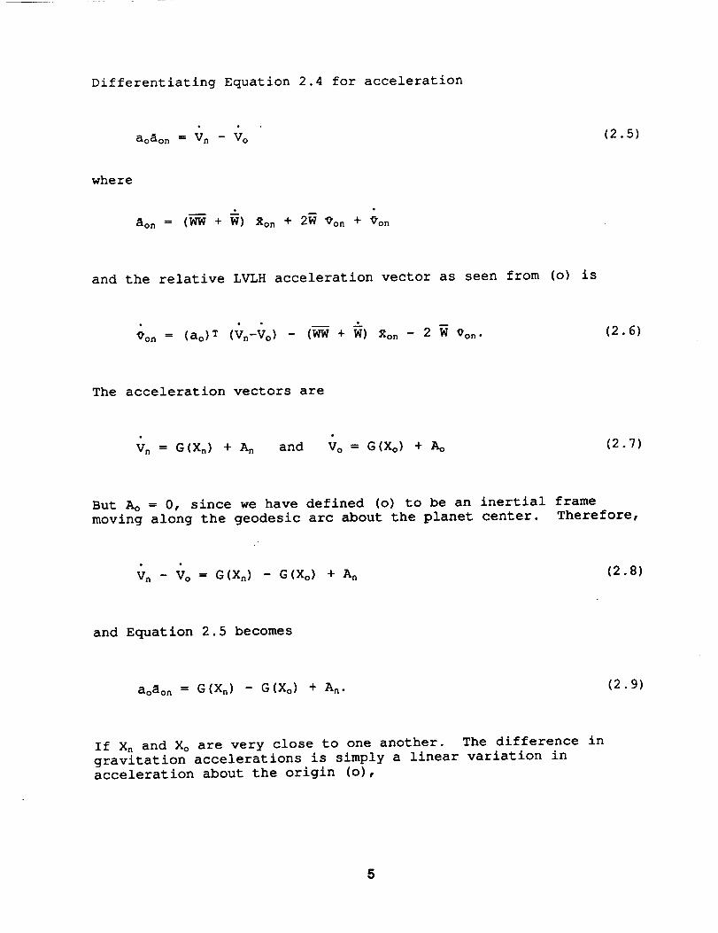
Differentiating Equation 2.4 for acceleration

ao_on = Vn - Vo (2.5)

where

_L"

aon = (WW + W) Son + 2W 9on + Con

and the relative LVLH acceleration vector as seen from (o) is

Con = (ao) T (Vn-Vo) - (WW + W) Son - 2 W Con. (2.6)

The acceleration vectors are

V, = G(Xn) + A n and Vo = G(Xo) + Ao (2.7)

But Ao = 0, since we have defined (o) to be an inertial frame

moving along the geodesic arc about the planet center. Therefore,

V n - V O = G(Xn) - S(Xo) + A n (2.8)

and Equation 2.5 becomes

aoaon = G(Xn) - G(Xo) + An. (2.9)

If Xn and Xo are very close to one another. The difference in

gravitation accelerations is simply a linear variation in

acceleration about the origin (o),

5

_G(Xo) ---G(Xn) - G(Xo)

and

_3

8G(Xo) = 6Xo =

8Xo

(Xn-Xo) --- Px (Xn-Xo) , (2.10)

therefore, Equation 2.9 becomes

aoaon = Px (Xn-Xo) + An- (2 .II)

From Equation 2.3 we have

aoaon = Px (aoXon) + An (2.12)

and solving for the acceleration in the LVLH frame,

Aon = [ (ao)TPx ao] Xon + (ao)TAn (2.13)

k D

aon = Px Xon + An (2.14)

where

D m

An = (ao)TAn and Px = [ (ao)TPx ao].

I

The Px matrix is defined from the similarity transformation for

matrices as described in Reference 5.0, Pages, 317 and 318, then

Equation 2.14 becomes,

D

9on = (Px-WW-W) Xon - 2W 9on + An. (2.15)

Equation 2.15 is the equation for motion for mass m in the LVLH

coordinates system attached to the geodesic point (o) in Figure

1.0. The Px matrices are used here for simplicity and also

contribute to understanding in the analysis, however, it should be

pointed out that the _x matrices are non-linear and their region of

numeric stability about the geodesic origin is small. Hence, for

very accurate relative motion computations the difference

equations of Equation 2.9 become a more reliable relationship on

which to base computational algorithms. Equation 2.15 can be

represented by the sum of two vectors,

9on = AIn + An, (2.16)

m

where Ain are the combined gravitational and inertial accelerations

effecting the relative motion of the center of mass.

w

The Px matrix reduces to (see Appendix C)

i 001 001Px = -_R-3 1 0 = -_ 1 0 . (2.17)

0 -2 0 -2

In a spherical gravitational field, i.e., where all gravity

harmonics are assumed zero,

7

WW =E°°IE°!°I[!oo0 0 0 - 0 0

o 0 0 o 0 0 -m{,

(2.18)

and for uniform circular orbit motion

W = 0. (2.19)

However, in the "real world" small oscillatory motions do occur

about the LVLH axes due to the gravity harmonics. Then Equation

2.15 reduces to

z 3m_ _- - 2m o 9 x +

n m

= AIx + A x

= Aiy + Ay

A z = Aiz + A z

(2.20)

which are recognized as the Clohessy-Wiltshire approximation for

the differential equations of relative motion [as described in

Reference 1.0]. The AI in Equation 2.20 are the combined relative

gravitational and inertial acceleration effects in the LVLH

system.

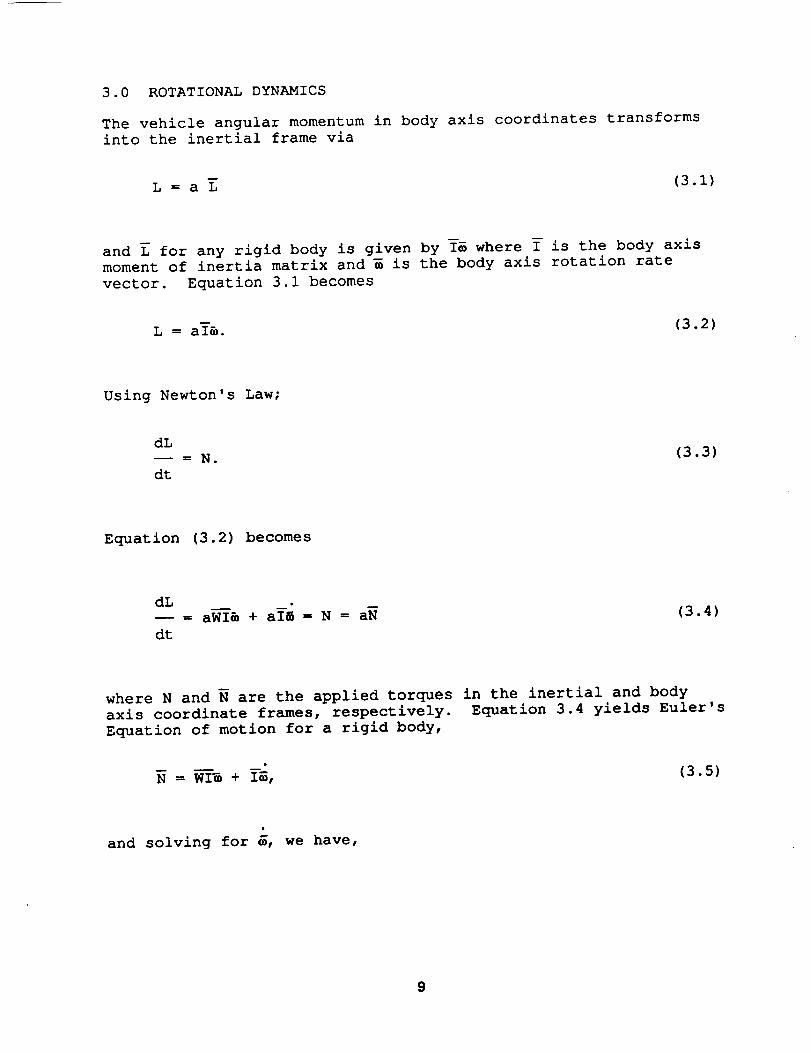
3.0 ROTATIONALDYNAMICS

The vehicle angular momentum in body axis coordinates transformsinto the inertial frame via

D

L = a L (3. I)

and L for any rigid body is given by I_ where I is the body axis

moment of inertia matrix and _ is the body axis rotation rate

vector. Equation 3.1 becomes

m

L = aI_. (3.2)

Using Newton's Law;

dL

== N.

dt

(3.3)

Equation (3.2) becomes

dL

_i --= aWI& + a = N = aN

dt

(3.4)

where N and N are the applied torques in the inertial and body

axis coordinate frames, respectively. Equation 3.4 yields Euler's

Equation of motion for a rigid body,

(3.5)

and solving for _, we have,

9

= J (N-WI_) (3.6)

where J = I-I, is the inverse of the body axis moment of inertia

matrix. The applied torques are composed of

N = NG + NT + NA + Np (3.7)

gravity, thrusting, aerodynamic and plume impingement torques,

respectively, and Equation 3.6 becomes

= J [NG + N T + N^ + Np + NI] (3.8)

where the inertial torques are N I = -WI_, which results due to

rotational motion of the vehicle itself. Integrals of this

equation [see Reference 3.0] provide the body axis rotation ratevector as a function of time.

I0

4.0 SIX DEGREES-OF-FREEDOM EQUATIONS OF MOTION

From Equation (2.20),

go

$n ------ _ mn + A--in

Wn

(4.1)

for translational dynamics and Euler's equation

= Jn (Nn - Wn In _n) (4.2)

for rotation dynamics, where;

go

Wn

Summation of contact forces acting on vehicle n

(LVLH Ref)

m

AIn " Inertial and gravitational accelerations of CM

of vehicle n (LVLH Ref)

m

I,

m

Jn

- Moment of inertia matrix of vehicle n

- Inverse of moment of inertia matrix of vehicle n

I

Nn " Body axis torques about the CM of vehicle n

D

Wn " Skew symmetric angular velocity matrix

(vehicle n)

- Body axis rotation rate vector (vehicle n)

- Body axis rotation rate acceleration vector for

vehicle n.

11

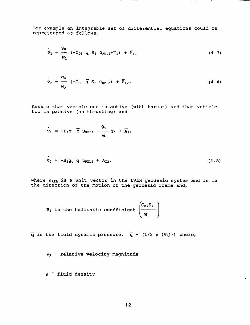
For example an integrable set of differential equations could berepresented as follows,

go

91 = -- (-CDI q S1 QRELI+TI) + AII

WI

(4.3)

go

92 = -- (-CD2 q $2 QREL2) + AI2.

W2

(4.4)

Assume that vehicle one is active (with thrust) and that vehicle

two is passive (no thrusting) and

• go

91 = -B1go q URELI + -- TI + AI1

WI

m

92 = -B2go q UREL2 + AI2, (4.5)

where URZL is a unit vector in the LVLH geodesic system and is in

the direction of the motion of the geodesic frame and,

Bi is the ballistic coefficient ICDiSi 1w±

m

q is the fluid dynamic pressure, q = (1/2 p (VR)2) where,

VR - relative velocity magnitude

p - fluid density

12

and the OREL vector in the LVLH reference frame is approximately,

UREL -----li°I0 .

0

(4.7)

With the above example in mind, Appendix A shows a suggested

integrable parameter list for a time-wise step solution to the

problem. More precise equations of motion can be defined by

computing the driving values for Fn and Nn in Equations 4.1 and

4.2, respectively, however, the same 6-DOF solution procedures

will apply.

13

5.0 TRANSLATION CONTROL PARAMETERS

As in Figure 2-1, the geodesic center is the motion of an

imaginary point falling along the local gravity geodesic arc. No

drag or other contact forces are acting at the geodesic center.

The rotating LVLH coordinate axes are attached to the geodesic

center. The position vector in the inertial coordinate system to

a point in space can be computed from each of the coordinate

systems shown in the following figure.

X1

X1

(nl)

LVLH

1

m

Xol

(o)

m

Xo2(n=) m

X2

PLANET CENTER

X

Figure 5-1

14

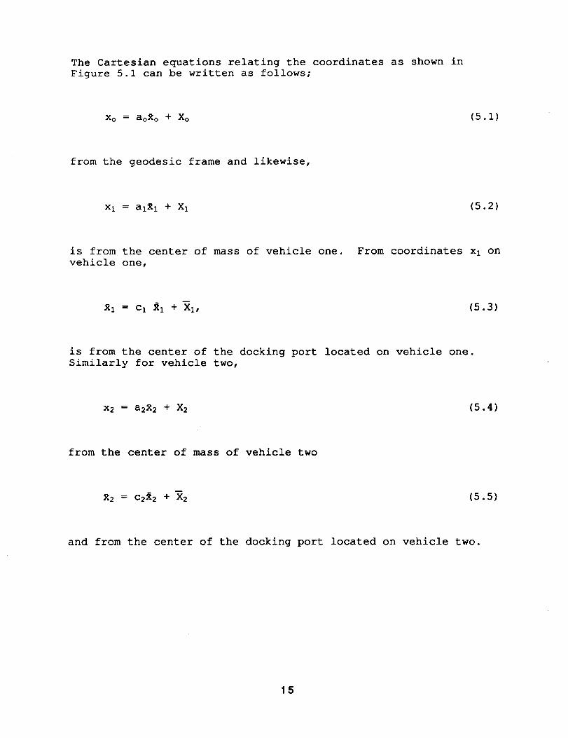
The Cartesian equations relating the coordinates as shown in

Figure 5.1 can be written as follows;

Xo = aoXo + Xo (5.1)

from the geodesic frame and likewise,

xl = alXl + Xl (5.2)

is from the center of mass of vehicle one.

vehicle one,

From coordinates xl on

I

_i -- ci _i + XI, (5.3)

is from the center of the docking port located on vehicle one.

Similarly for vehicle two,

x 2 = a222 + X 2

from the center of mass of vehicle two

(5.4)

I

X 2 = C2_ 2 + X 2 (5.5)

and from the center of the docking port located on vehicle two.

15

The following definitions apply to Equations 5.1 through 5.5

ao - The LVLH to inertial transformation matrix attached to

the geodesic coordinate center (a time varying matrix)

al - i TM body axis to inertial transformation matrix

(a varying matrix)

X i " The inertial coordinates of the ith coordinate center

(a dynamic vector in motion about the planet center)

ci - i th docking port to body axis transform matrix

(a constant matrix)

X--i - Body axis coordinates of the ith body docking port

coordinate center (a constant vector).

The target docking port inertial position is

XT = a2 _2 + X2

Xw = a2 (c2_2+X2) + X2 (5.6)

but

X2 = 0,

since the target is the docking port coordinate center and

therefore Equation 5.6 reduces to

m

XT = a2 X2 + X2, (5.7)

the target location in inertial coordinate. Hence, the position

relative geometry in the inertial coordinate reference frame

becomes

16

a2 X2 + X2 = al (cl_l+Xl) + Xl (5.8)

from Equation 5.1

Xl -- aoXol + Xo and X2 = aoXo2+ Xo (5.9)

and substituting these into Equation 5.8

a2X2 + aoXo2= al (cl Xl+Xl) + ao Xol (5.10)

where the _o2 and Xo2 are the position vectors to the vehicle oneand two center of mass measured in the LVLH geodesic coordinateframe of reference.

By multiplying Equation 5.10 by the transformation matrix (ao) T,the equation is transformed to the LVLH frame,

(ao) T a2 X2 + Xo2 = (ao)T az (czRli-Xz.) + R.o2. (5.11)

Now let bl = (ao)Tal and b 2 = (ao)Ta2, be the transformation matrices

for the body axes to the LVLH reference frame. Then Equation 5.11

becomes

D

(Ro2- R.ol) = bl (Cliz+Xl) - b2X2' (5.12)

the relative position vector between the two vehicles in the LVLH

frame and solving for El,

41 = (cl)T[ (bl)T{ (Xo2-Xol)+b2X2} - Xl] • (5.13)

17

We have the position control vector as seen from the vehicle one

docking port coordinate center. The GN&C systems should drive

this vector to zero for docking contact. Written in body axis

coordinates we have,

Xl = ClXl = (bl) T (b2_2+ (Ro2-Rol)) - Xl, (5.14)

the control vector as seen from the active vehicle (vehicle one).

Hence, a candidate commanded velocity in the vehicle frame

becomes,

9 c = K R R 1 (5.15)

where the gain,

KR = --

can be applied in an Flight Control System (FCS) with appropriate

limiters for proper closing rates. For the velocity of the target

docking port we differentiate Equation 5.9

a2W2X2 + aoWoXo2 + ao9o2 = aiWl (cIXI+XI)

m

+ alCl91 + aoWoRol + ao$ol. (5.16)

Again by multiplying by (ao) T the equation is reduced to LVLH

coordinates,

18

(ao)Ta2W2 X2 + WoXo2 + 902 = (ao)TaiW1 (clRI+XI)

+ (ao)TalCl_l + WoRol + 9oi (5.17)

and the relative velocity difference in the LVLH frame is,

w _ m

(9o2-9ol) = blWI(clXI+XI) + bic1_i - b2W2X2 - Wo(Xo2-Xol) (5.18)

and the docking port relative velocity of the docking port

coordinate center on vehicle two (the target) is

91 = (Cl)T[ (bl)T{ (9o2-9ol)+Wo(Xo2-Xol)+b2W2X2}-WI(ClXI+Xl) ] • (5.19)

The control velocity vector in vehicle body axis coordinates

becomes,

91 = cl_l = (bl) T [ (9o2-9oi) +Wo (Xo2-Xol) +b2W2X2 ] -WI (Cl_l+Xl) . (5.20)

Using Equations 5.15 and 5.20, the AV command for translation

control becomes,

I

AVc= _'c - 91, (5.21)

and when applied with appropriate limiters or closing gates, the

algorithm can be used to the control closing conditions for safe

docking. The acceleration of the control vector is found by

differentiation of Equation 5.16 and becomes

19

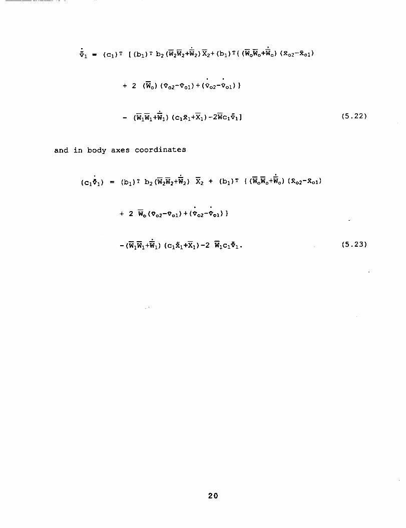
vz = (Cl) T [ (bl) T b2 (W2W2+W2) X2+ (bl) T{ (WoWo+Wo) (_o2--_.ol)

+ 2 (Wo) ('_o2-';'ol) + (%2-%1) }

- (WzWI+WI) (CIRI+Xl)-2Wc191] (5.22)

and in body axes coordinates

(cl@l) = (bl) T b2 (W2W2+W2) X2 + (bl) T { (WoWo+Wo) (Xo2-Xol)

+ 2 Wo (O'o2-_'oZ) + (_'o2-O'oz) }

- (W1WI+WI) (cl_I+'Xl)-2 WICI_'].. (5.23)

20

6.0 ROTATION CONTROL PARAMETERS

The attitude control matrix may be derived as from rotation

equations as follows

X 1 = al_ 1 x2 = a2_ 2

_I == Cl_l _2 = c2_2

xl = [alcl] RI x2 = [a2c2]R2 (6.1)

The desired attitude condition at docking is that the two systems

have approximately the same orientation in inertial space and,

therefore,

alcl --"a2c2. (6.2)

If vehicle number one is the active control vehicle,

al_ = a2c2 (cl) _ (6.3)

is the desired attitude matrix for vehicle number one.

control matrix becomes

The

alXl = aldXld

Xl ----[ (al)Tald]Xld

Ri = [ (ai) Ta2c2 (Cl) T] Rid

CN = [ (ai)T a2c2 (ci)T] (Attitude Control Matrix) (6.4)

21

That is, the CN matrix will become the unit matrix when the dockingports are aligned. By extracting the Hamilton Quaternion from the

CN matrix a desired rotation can be found to align the docking

ports as follows;

ql

q2I=

,q4 J

'COS (m12)

sin (m12) cosa

sin (m12) cos_

sin (_12) cos7

(6.5)

where

m = 2 cos -I (ql), (6.6)

is the instantaneous angular control rotation required to alignthe docking ports.

The eigen axis about which the controlled rotation of vehicle one

must occur becomes

cosa ] 1 " q2

== q3 •sin (e/21

kcos7 ] q4

(6.7)

Hence, as m approaches zero, the CN matrix approaches the unit

matrix and the desired attitude condition of Equation 6.4 can be

reached. The vehicle one attitude GN&C functions must be designed

to control the spacecraft to this desired attitude.

The soft singularity indicated in Equation 6.7 will not be reached

since m will fall into the control attitude deadband before m - 0.

A candidate commanded body axis rate vector may be estimated by

selecting a scaler quantity _ for the desired angular closing rate

for the control quaternion and the desired body axis rotation ratebecomes

22

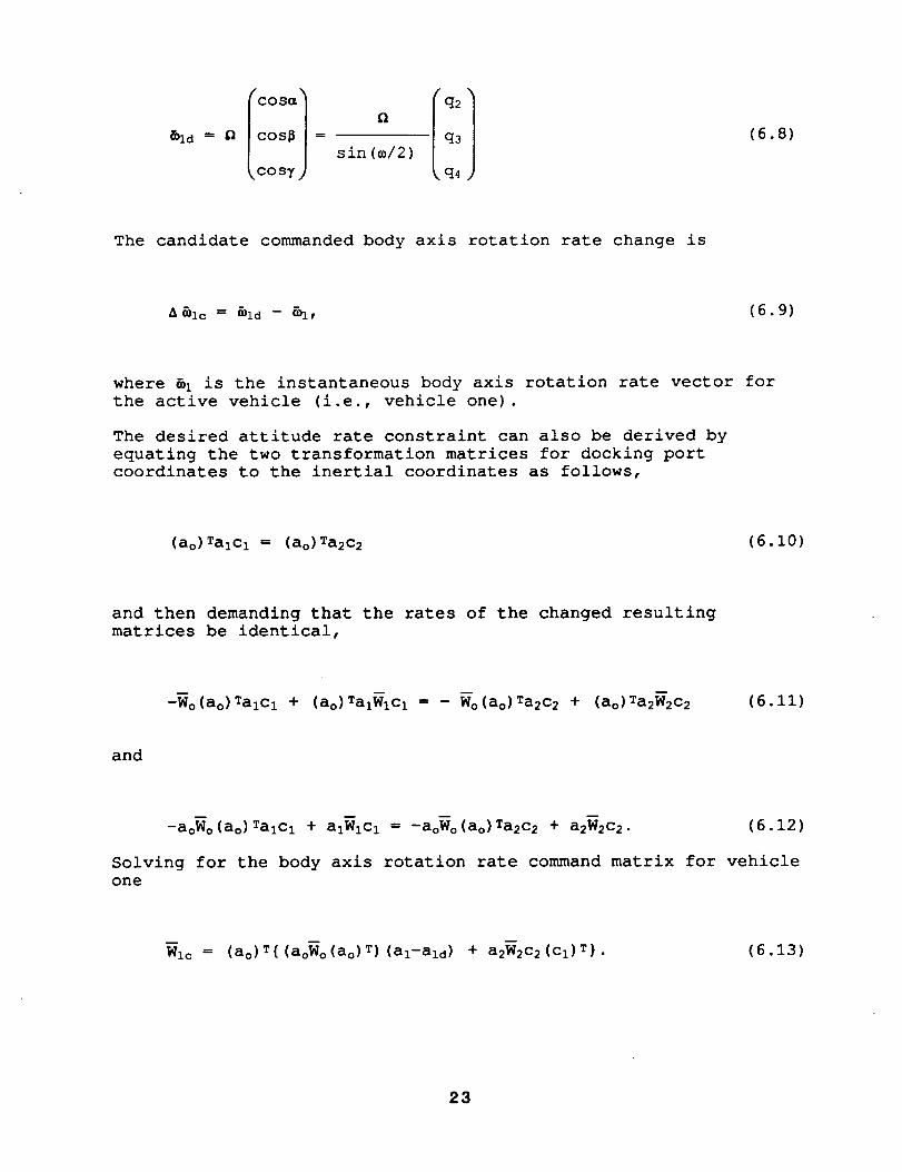
olq21kCO s7 ] q4

The candidate commanded body axis rotation rate change is

A _Ic = _id -- _I, (6.9)

where _i is the instantaneous body axis rotation rate vector for

the active vehicle (i.e., vehicle one).

The desired attitude rate constraint can also be derived by

equating the two transformation matrices for docking port

coordinates to the inertial coordinates as follows,

(ao) Talcl = (ao) Ta2c2 (6.10)

and then demanding that the rates of the changed resulting

matrices be identical,

-Wo(ao) Talcl + (ao)TaiWlcl = - Wo (ao)Ta2c2 + (ao)Ta2W2c2 (6.11)

and

-aoWo(ao) Talcl + aIWlcl = -aoWo (ao)Ta2c2 + a2W2c2. (6.12)

Solving for the body axis rotation rate command matrix for vehicle

one

Wlc = (ao)T{ (aoWo(ao) T) (al-ald) + a2W2c2(cl) T}. (6.13)

23

The ald matrix is the desired attitude matrix given by Equation

6.3. Note that when the al matrix approaches the ald (desired

attitude matrix) the steady state rotation rate command matrix for

vehicle one becomes

Wlc = (al)Ta2W2C2(Cl)T.

The candidate FCS could monitor the error signal, (al-ald) from

Equation 6.13 above and apply appropriate gains and limiters to

control the attitude of vehicle one during docking.

24

7.0 CONCLUSIONS AND RECOMMENDATIONS

Detailed analysis of the Automatic Rendezvous and Capture problem

indicate three different regions of mathematical description for

the GN&C algorithms; (I) multi-vehicle orbital mechanics to the

rendezvous interface point, i.e., within I00 NM, (2) relative

motion solutions (such as Clohessy-Wiltshire type) from the far

field to the near field interface, i.e., within 1 NM and (3) close

proximity motion - the near field motion where relative

differences in the gravitational and orbit inertial effects can be

neglected from the equations of motion. Limit boundaries to these

regions can be precisely defined by further analysis and will also

be a function of the tracking measurement accuracies and the

computer resources available to the solution algorithms.

The subjects of this paper analyze the regions (2) and (3) above

and presents the derivation and discussion of the general case of

gravitational perturbed relative motion. Mathematical deviations

from the spherical gravity case of Clohessy-Wiltshire are

presented in the analysis. Based upon the preliminary analysis ofthis work it is recommended that further efforts be used to assess

the relative position and velocity differences in region (2) due

to non-spherical effects (especially that of J2) in the gravity

perturbations. Future GN&C systems using relative motion

measurements from either an onboard laser tracking systems or from

the GPS will possibly be able to detect and predict these

perturbations in the relative motion.

The docking port relative position and velocity target vectors as

outlined in this work couples the effects of the translation and

rotation control activity. Based on these preliminary control

parameters it is recommended that guidance and control systems

functions couple translation and attitude control in region (3)

for safe docking maneuvers. In region (2) the relative range

between the docking port targets is assumed large enough so that

translation and rotation G&C functions can be independent of one

another.

25

8.0

[1]

[2]

[33

[4]

[5]

REFERENCES

W. H. Clohessy and R. S. Wiltshire, "A Terminal Guidance

System for Satellite Rendezvous," Aero/Space Science, Vol. 27,

Pg. 653, September 1960.

Pedro Ramon Escobal, "Methods of Orbit Determination," John

Wiley & Sons, Inc., 1965.

David Henderson, "Solution of Euler's Equations of Motion for

a Rigid Body Using the Quaternion," presentation at

JSC/Houston, TX, AIAA Technical Mini Symposium, March 21,

1978.

Harry Lass, "Vector and Tensor Analysis," McGraw-Hill Book

Company, Inc., 1950.

Henry Margenau and George Murphy, "The Mathematics of Physics

and Chemistry," (Second Edition), D. Van Nostrand Company,

Inc., Pg. 317-318, January 1956

26

SUGGESTED INTEGRABLE PARAMETER LIST

APPENDIX A

The following list contains the fundamental parameters necessaryto solve for the motion and attitudes of two vehicles relative to

the geodesic LVLH frame and the body axis frame, respectively. A

numerical process to perform the first order solution of this set

of simultaneous differential equations is required. This process

will perform the integral

x(t+_t) = x(t) + dt.

The process of Runge-Kutta-Gill is recommended, however, in some

applications requiring high frequencies (i.e., small At) the Cauchy-

Euler solution method is adequate for an accurate solution.

27

Suggested list

x(t) x(t)

Vehicle

Number

One

Vehicle

Number

Two

I ,

2.

3.

4.

5.

6.

7.

8.

9.

10.

II.

12.

13.

14.

15.

16.

17.

18.

19.

20.

21.

22.

23.

24.

25.

26.

Xol

_oI

ql

(Position)

LVLH Ref.

(Velocity)LVLH Ref.

(Quaternion)

(Body axis to

inertial)

(Body Axis

Rotation Rates)

:_o2

'0'o2

q2

"qol

go--BIqgoOVREL + -- TI + All

WI

ql

Ji (NI-WI II&1 )

_'o2

D

--B2_goUvREL + AI2

(_2

J2 (N2-W2 I2¢2 )

In the event that the absolute inertial state is required, the

following additions can be made to the integrable parameter list

Inertial

StateI 27.

28.

29.

30.

31.

32.

Xo

Vo

x(t) _(t)

Vo

Go --- V O

where Go is the acceleration due to gravity at the point Xo, the

geodesic coordinate center (see Figure 2-1).

28

GRAVITATIONAL ACCELERATIONS

APPENDIX B

Using the Newtonian formulation of gravity the inertial

gravitational acceleration vector in a spherical gravity field is

G(x) = -_R-3 x (B.I)

where x is the column vector for position from the gravitating

mass center, that is,

Ixlx = y . (B.2)

z

To transform B.I into the LVLH coordinate frame use Equation 2.1

in B.I,

G(R) = - _R-3aoR - _R-3 x o (B.3)

and transform G(R) to the LVLH frame,

(ao)TG(X) = G(R) = - _R-3(X) - _R-3(aTXo) . (B.4)

Since the LVLH coordinate axes are aligned with the Z-axis in the

-R direction, Equation B.4 reduces to

G(x) = - _R-3

2-Ro

(B.5)

29

The gravitational acceleration vector in a field perturbed by non-

spherical gravity harmonics, we write,

G(x) = - _R-3 (I+_)x (B.6)

where I is the unit matrix an • is a diagonal matrix,

= _O _Y0 _z0 (B.7)

For example, using the J2 harmonic only as shown in Reference 2,

Pages 50 and 51,

_X

I III312 2 II1sR3/2 J2 3-5 R

(B.8)

Here, RE is the reference planetary equatorial radius and J2 is the

first zonal harmonic. For instance, the J2 harmonic for the earth

is -I.0826271xi0 -2 (unitless) and has the most pronounced effect on

the motion of the low earth orbit spacecraft.

n

Transforming G(x) in Equation B.6 into G(R) we have

where I is the unit matrix and _ is given by the similarity

t rans format ion,

3O

= a T _ a, (B.10)

and becomes a full matrix in the LVLH coordinate frame. Using the

J2 harmonic only from Equation B.8 and reducing to LVLH coordinates

Equation B.9 becomes,

IaT[K]a-5 IRIIII [i_Rol(B.II)

where the matrix [K] is a constant matrix given by

[K] =

i.0 0 0 ]

0 1.0 0 •

0 0 3.0

(B.12)

81

PARTIAL DERIVATIVES OF THE

GRAVITATIONAL ACCELERATION VECTOR

APPENDIX C

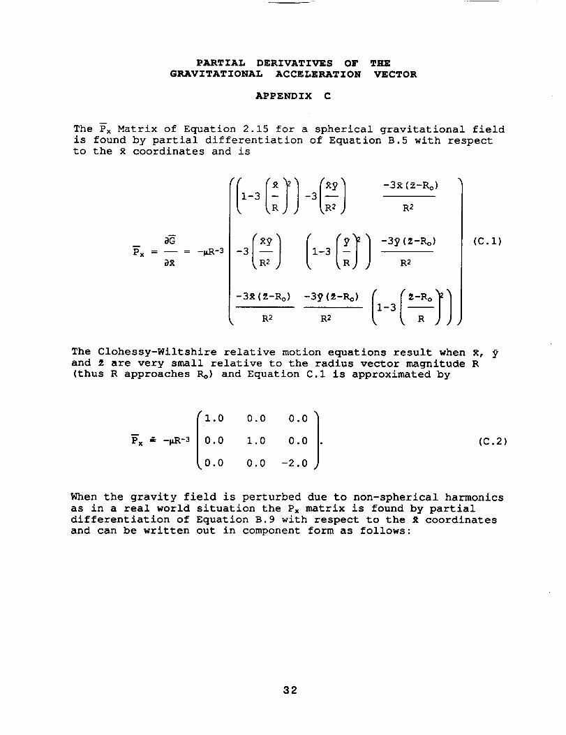
The Px Matrix of Equation 2.15 for a spherical gravitational field

is found by partial differentiation of Equation B.5 with respect

to the X coordinates and is

aG

Px .... _R-3

%X

-3£ (2-Ro)

R 2

-3R (2-Ro) -3 9 (2-R o)

R 2 R 2

(C.l)

The Clohessy-Wiltshire relative motion equations result when X,

and 2 are very small relative to the radius vector magnitude R

(thus R approaches Ro) and Equation C.I is approximated by

I.0 0.0 0.0 1

Px --"-MR-3 0.0 1.0 0.0 . (C.2)

0.0 0.0 -2.0

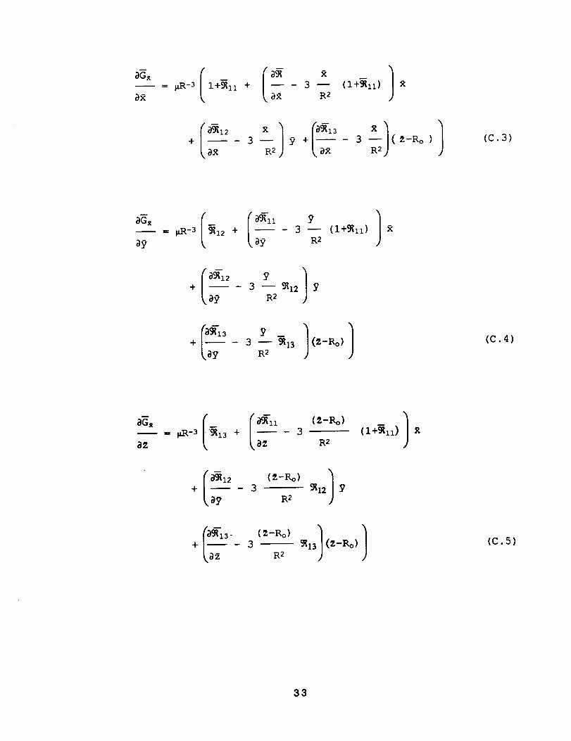
When the gravity field is perturbed due to non-spherical harmonics

as in a real world situation the Px matrix is found by partial

differentiation of Equation B.9 with respect to the R coordinates

and can be written out in component form as follows:

32

I I%G_ _LR-3 i+_11 + 3-

aX _X R 2

m

_12 X

R2( _-Ro ) (C.3)

m

_)Gx

a9I I-_12 +

_9

3--R2

(i+9_ii)

+ -- 3 -- _12 Y

kay R2

-- 3 -- _13 (Z-Ro)

_ay R2

(C.4)

1

a,. ka_.

(_--Ro)

3R2

(l+_n)

+ _i2 (Z-Ro) )-- 3 _12

_,a9 R2

Y

-- 3 _13

_a_ R2

(_-Ro) (C.5)

33

%R

= _R-3I I-_21 + 3

R2

+ / C_'_22

R2(1+_22)

+ la_-23 z-- 3 -- 9_2a

_ax R2(C.6)

-- = _R-3 1 + 9_22+ --a9 _,a9

Y3--

R2

I o_22 9'+ -- 3 --a:_ R2

( 1 +'_'_2 2 )9

+ , ) )3 -- _23R2

(C.7)

-- __ fAR-3

(2-Ro)3

R 2(l+Rn)

,_22 (Z-Ro)+ -- 3

aZ R 2(I+C_22)

+a_Tn (Z-Ro) 1-- 3 _23

La_ R2(_--Ro ) (C.8)

34

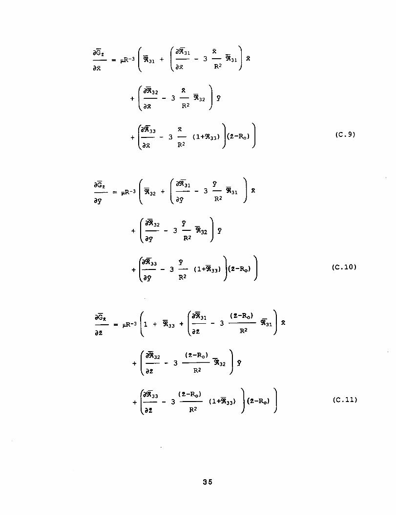
aGz

-- _ jlR-3 I Ia_1_31 + --

%X

3 -- _31

R 2

R

+i __

o-_32

3 -- _32

R2

3

_,a_ R2

(1+_33)(C.9)

B

%Gz

a_[ I_I_32 + --

a_

3 -- _31 £

R2

+ , )3 -- _32R2

+ , ) )3- (i+_33) (Z-Ro)

R 2

(c.10)

C__aGx = I_R-3 1 + _33 + 3 W3_

_az R2

+a_n (Z-Ro) _ 1- 3 _32 9

_2 R 2

+

(Z-Ro)

3 (I+_33)

R2/ (Z-Ro) ) (c.11)

35

As R, @ and 2 approach zero (R approaches Ro) and Equations C.3

through C.II form the _x matrix as in Equation C.2 but for non-

spherical case,

_:, -- -_,_-3

l+_ll-R° -- -- --

_31-Ro -- 32-Ro 2 +2_33-R o

(C.12)

Typical values for the Px matrix in a 4x4 gravity field at 190 NM

altitude (orbit inclination 28.5") as a function of orbital

longitude (L) are;

For L = 0.0",

(Px = -_LR-30.100211132E+1 -0.127455301E-2 0.860795280E-4 |

J-0.127455552E-2 0.I00374459E+I 0.141282142E-5

0.441508313E-4 -0.992324472E-4 -0.200586443E+1

(C.13)

For L -- 91. 914"

( 1-- 0. 999755725E+0 0. 656077200E-4 -0.128398836E-3

Px = -p/_-3 0.658219319E-4 0.100197258E+1 -0.497582344E-2

-0.780933175E-4 -0.490363083E-2 -0.200185338E+1

(C.14)

For L = 184.114"

0.I00217612E+I

0.I19982659E-2

0.223653423E-30.119984812E-2 0.174780536E-3 10.I00371725E+I 0.414833236E-3

0.303452941E-3 -0.200589351E+1

(C.15)

For L = 276.309"

\0.999822606E+0 -0.917771447E-4 -0.183744890E-3 |

J-0.916192270E-4 0.I00211408E+1 0.474542054E-2

-0.217657097E-3 0.482754340E-2 -0.200180233E+1

(C.16)

36

REPORT DOCUMENTATION PAGEForm Approved

OMB NO. 0704-0188

Pubh( reporting our_en for this collection of information rS estimated to average 1 hour oer res_onse, indu¢ling the time for reviewing irlsti'uctlofls, searching existing data sources,

gathering and maintaining the data neecle_i, anO ¢omDietlng aria reviewing the collection of information SenO comments regarding this burden estimate or anv other asDect of th,s

collection Of intot'matton, _ncJu_lng suggestions for re_<lng _hls _uraen to Washington Heaa_uarter$ Services. D(redorate for _ntorma_on O_ratlons ariel Repotls. 12 _5 Jefferson

Daws Highway, Su*te 1204, Arlington, VA 22202-4302. and to the Off,ce of Management and Budget. Paperwork Reduction Pro ect (0704-0188), Washington, DC 20503.

1. AGENCY USE ONLY '{Leave blank) 2. REPORT DATE

April 19924. TITLEANDSUBTITLEReference EquationsAutomatic Rendezvous

6. AUTHOR(S)

David M. Henderson

of Motion for

and Capture

7. PERFORMING ORGANIZATION NAME(S) AND ADORESS(ES)

3. REPORT TYPE AND DATES COVERED

Technical Re)ort5. FUNDING NUMBERS

NAS9-17900

i

8. PERFORMING ORGANIZATION

TRW Systems Services Company,P.O. Box 58327

Houston, Texas 77258

Inc.

9.SPONSORING/MONITORINGAGENCY NAME(S)AND ADDRESS(ES)

National Aeronautics and Space Administration

Lyndon B. Johnson Space CenterHouston, Texas 77058

REPORT NUMBER

TRW Report No.91:J431.1-182

10. SPONSORING/MONITORING

AGENCY REPORT NUMBER

NASA CR 185676

11. SUPPLEMENTARY NOTES

12a.OISTRIBUTION/AVAILABILITYSTATEMENTUnlimited

Publicly Available

12b. DISTRIBUTIONCODE

Subject Catagory13

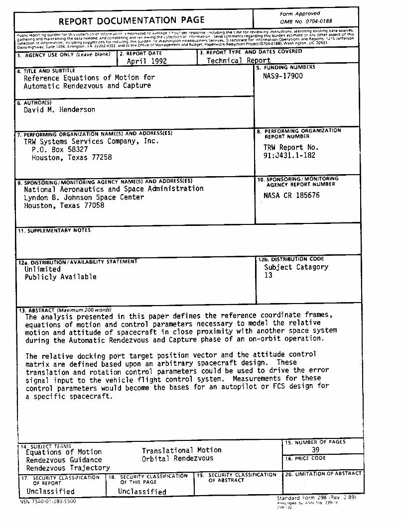
13. ABSTRACT (Maximum 200 wor_)

The analysis presented in this paper defines the reference coordinate frames,

equations of motion and control parameters necessary to model the relative

motion and attitude of spacecraft in close proximity with another space system

during the Automatic Rendezvous and Capture phase of an on-orbit operation.

The relative docking port target position vector and the attitude control

matrix are defined based upon an arbitrary spacecraft design. Thesetranslation and rotation control parameters could be used to drive the error

signal input to the vehicle flight control system. Measurements for these

control parameters would become the bases for an autopilot or FCS design fora specific spacecraft.

14 SUBJECTTER._ISEquations of Motion Translational MotionRendezvous Guidance Orbital Rendezvous

Rendezvous Trajectory

17. SECURITY CLASSZFfCATION J.18. SECURITY CLASSIFICATION lg. SECURITY CLASSIFICATION

OF REPORT I OF THIS PAGE OF ABSTRACTUncl assi fied Unclassi fied

NSN 75_.0-0_ -280-5500

15. NUMBER OF PAGES

3916. PRICE CODE

20. LIMITATION OF ABSTRACT i

Stanclard ;orm 29B {Rev 2-89)

Z'4_.'_ 32