18.305 lecture notes: stochastic...

18.305 Lecture Notes:

Stochastic Calculus

Homer Reid

December 8, 2015

Abstract

Contents

1 Motivation 2

2 Stochastic Variables 32.1 Stochastic Variables . . . . . . . . . . . . . . . . . . . . . . . . . 32.2 Probability densities, cumulative probabilities . . . . . . . . . . . 32.3 Moments and characteristic functions . . . . . . . . . . . . . . . . 52.4 Vector-valued stochastic variables . . . . . . . . . . . . . . . . . . 62.5 Multidimensional Gaussian stochastic variables . . . . . . . . . . 72.6 New random variables from old . . . . . . . . . . . . . . . . . . . 72.7 The discrete Wiener process . . . . . . . . . . . . . . . . . . . . . 8

3 Stochastic Processes 113.1 Gaussian stochastic processes . . . . . . . . . . . . . . . . . . . . 113.2 The Wiener process . . . . . . . . . . . . . . . . . . . . . . . . . 12

3.2.1 Probability of hitting specific values . . . . . . . . . . . . 123.2.2 Mean-square variation from time t to t+ ∆t . . . . . . . . 13

4 Stochastic calculus 144.1 Stochastic integrals . . . . . . . . . . . . . . . . . . . . . . . . . . 14

4.1.1 Stochastic integrals a la Ito . . . . . . . . . . . . . . . . . 144.1.2 Stochastic integrals a la Stratonovich . . . . . . . . . . . . 14

4.2 Stochastic ODEs . . . . . . . . . . . . . . . . . . . . . . . . . . . 14

5 Other processes 145.1 Poisson process . . . . . . . . . . . . . . . . . . . . . . . . . . . . 145.2 Levy process . . . . . . . . . . . . . . . . . . . . . . . . . . . . . 155.3 Ornstein-Uhlenbeck process . . . . . . . . . . . . . . . . . . . . . 155.4 White noise . . . . . . . . . . . . . . . . . . . . . . . . . . . . . . 15

1

18.305 Lecture Notes 2

A Green’s function approach 16A.1 Statistical solution of ODEs subject to stochastic forcing terms . 16A.2 Causal Green’s function for a 1D particle in a viscous fluid subject

to a harmonic restoring force . . . . . . . . . . . . . . . . . . . . 16A.3 Fluctuations of a Brownian particle in a harmonic trap . . . . . . 17


1 Motivation

Everything we have discussed in 18.305 has been essentially deterministic innature: we have exclusively solved ODEs with deterministic forcing functions,we have exclusively evaluated integrals with deterministic integrands, etc. Inthis, our approach has been in keeping with the general strategy of the greatmajority of courses in mathematics, science, and engineering: we teach you allthe deterministic stuff, but relegate stochastics to the status of an afterthoughtor secondary advanced topic.

In the second half of the 20th century there developed an increasing aware-ness among researchers and educators that this approach was fundamentallyunsuited to the nature of modern research, in which most interesting problemsinvolve stochastic entities. This may be because the very nature of the problemin question is unavoidably stochastic at heart—as is true, for example, in thestudy of diffusion processes and other fluctuation-induced phenomena—or itmay be simply because probabilistic methods are often the best way of solvingdeterministic problems, a phenomenon in evidence across a wide range of fieldsfrom graph theory to computational particle physics.1 In the same way thatphysics educators of the 1930s were forced to undertake a thorough revampingof their curricula, which had been rendered quaint and outdated by the adventof quantum mechanics, there will come a day sometime in the early 21st centurywhen applied-math educators will have no choice but to reboot the canonicalcurriculum in such a way as to emphasize stochastic methods from the getgo.These notes may be thought of as a preliminary attempt to jumpstart this pro-cess by introducing some of elements of the mathematical toolbox known asstochastic calculus.

1For a particularly forceful, fascinating and erudite discussion of this point from a mas-ter of pure mathematics (and, by his own admission, a former skeptic regarding the utilityof probabilistic methods who is now a full Kool-Aid-drinking convert), see the essay “TheDawning Age of Stochasticity” by the famous algebraic geometry guru David Mumford:https://www.researchgate.net/publication/27298183_The_Dawning_Age_of_Stochasticity.

https://www.researchgate.net/publication/27298183_The_Dawning_Age_of_Stochasticity

https://www.researchgate.net/publication/27298183_The_Dawning_Age_of_Stochasticity


2 Stochastic Variables

2.1 Stochastic Variables

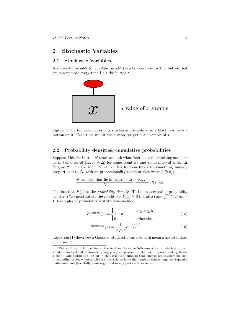
A stochastic variable (or random variable) is a box equipped with a button thatemits a number every time I hit the button.2

Figure 1: Cartoon depiction of a stochastic variable x as a black box with abutton on it. Each time we hit the button, we get out a sample of x.

2.2 Probability densities, cumulative probabilities

Suppose I hit the button N times and ask what fraction of the resulting numberslie in the interval [x0, x0 + ∆] for some point x0 and some interval width ∆(Figure 2). In the limit N → ∞ this fraction tends to something linearlyproportional to ∆, with an proportionality constant that we call P (x0) :

# samples that lie in [x0, x0 + ∆]

N

N→∞−−−−−→ P (x0)∆.

The function P (x) is the probability density. To be an acceptable probabilitydensity, P (x) must satisfy the conditions P (x) ≥ 0 (for all x) and

∫∞∞ P (x) dx =

1. Examples of probability distributions include

P uniform(x) =

1

b− a, a ≤ x ≤ b

0 otherwise(1a)

P gaussian(x) =1

σ√

2πe−

(x−µ)2

2σ2 . (1b)

Equation (1) describes a Gaussian stochastic variable with mean µ and standarddeviation σ.

2Think of the little machine at the bank or the driver’s-license office on which you pusha button and get out a number telling you your position in the line of people waiting to seea clerk. One distinction is that in that case the numbers that emerge are integers emittedin ascending order, whereas with a stochastic variable the numbers that emerge are typicallyreal-valued and (hopefully!) not organized in any particular sequence.


-1

-0.5

0

0.5

1

1.5

2

0 50 100 150 200 250 300

Val

ue o

f nth

sam

ple

Sample index nFigure 2: Values of 300 samples of a stochastic variable x, which in this caseare uniformly distributed throughout [0 : 1].


2.3 Moments and characteristic functions

Given a probability density P (x), I can compute its moments by evaluatingdefinite integrals. The most famous moments are the mean

〈x〉 =

∫ ∞−∞

xP (x) dx (2)

and the variance σ2 =⟨x2⟩−⟨x⟩2

where

⟨x2⟩

=

∫ ∞−∞

x2P (x) dx. (3)

More generally, the pth moment is

〈xp〉 =

∫ ∞−∞

xpP (x) dx (4)

Given a probability distribution P (x), it quickly gets annoying to have to eval-uate a separate integral for each separate moment. Because differentiation iseasier than integration, it’s convenient to define a gadget that I can differen-tiate p times to get the pth moment of my distribution. Such a gadget is thecharacteristic function of the probability density P (x), defined as a function ofan auxiliary variable s by

C(s) = 〈esx〉 =

∫ ∞−∞

esxP (x) dx.

The point of this definition is that it establishes C(s) as the generating functionfor the moments of the probability distribution:

〈xp〉 =dp

dspC(s)

∣∣∣∣s=0

.

Thus, knowledge of C(s) is equivalent to knowledge of P (x); one function en-codes all properties of the other function.3 The characteristic functions corre-sponding to the probability densities (1) are

Cuniform(s) =esb − esa

s(b− a), (5a)

Cgaussian(s) = e12σ

2s2+µs (5b)

3This is actually obvious from the fact that C(s) is just the Fourier transform of P (x)

evaluated at an imaginary argument, C(s) = 2πP̃ (is).


2.4 Vector-valued stochastic variables

An easy generalization of the stochastic-variable concept is the notion of a D-dimensional vector-valued stochastic variable. This is again a box with a button,but now whenever I hit the button I get not just a single number but D numbersx1, x2, · · · , xD: instead of just one:

Figure 3: A vector-valued random variable. Each time we hit the button, weget a vector of D numbers x.

Everything that we discussed above has an immediate and easy generaliza-tion to this case. For example, if I hit the button N times and ask for the fractionof outputs that live within a D-dimensional hypercube of side ∆ with one cornerat x0, I find that as N → ∞ this number tends to something proportional tothe hypercube volume ∆D:

# samples that lie in hypercube of side ∆ with vertex at x0

N

N→∞−−−−−→ P (x0)∆D

where the probability density must satisfy

P (x) ≥ 0 for all x ∈ RD and

∫P (x)dDx = 1

where the integral runs over all of RD.I can also generalize the concepts of moments and generating functions to the

multidimensional case. The various possible moments I can compute are nowindexed by D-dimensional vectors p = (p1, p2, · · · , pD) of integers (specifyingone power for each entry in the stochastic-variable vector) and I can write

〈xp〉 = 〈xp11 xp22 · · ·x

pdd 〉

=

∫xp11 x

p22 · · ·x

pdd P (x) dDx

which I once again think of as the derivative of generating function:

=dp1

dsp11

dp2

dsp22

· · · dpD

dspDDC(s)

∣∣∣∣s=0


with

C(s) ≡⟨ex·s

⟩=

∫ex·sP (x) dDx. (6)

Note that the meaning of the multivariable moment here is the following:I hit the button on my box N times, and from each vector that comes out Iextract the ath and bth components and add their product to a running sum.This sum, normalized by N , is the moment corresponding to the vector p with1s in the a, b slots and zeros in all other slots:∑∞

n=1 value of xaxb on nth sample

N

N→∞−−−−−→⟨xaxb

⟩(7)

2.5 Multidimensional Gaussian stochastic variables

To specify the probability density for a one-dimensional Gaussian stochasticvariable (1b) requires specifying two numbers: the mean µ and the standarddeviation σ (equivalent to specifying the variance σ2.) The D-dimensional ana-logue of this requires specifying a D-dimensional vector µ (whose componentsare the mean values of the components of the stochastic variable vector) and aD×D-dimensional matrix Σ, whose entries specify the covariances; the PDF is

P (x) =1√

(2π)D det Σe−

12 (x−µ)TΣ−1(x−µ) (8)

The mean values and covariances of the components of this vector-valued stochas-tic variable are ⟨

xn⟩

= µn,⟨xmxn

⟩= Σmn. (9)

If the Σ matrix is diagonal, then (8) just describes D independent Gaussianstochastic variables, with the dth variable having mean µd and standard devia-tion

√Σdd.

The moment generating function for the D-dimensional Gaussian stochasticvariable with mean vector µ and covariance matrix Σ is the multidimensionalgeneralization of (5b); now it is a function of a D-dimensional auxiliary variables:

C(s) = e12 sΣs+µ·s. (10)

2.6 New random variables from old

Given one stochastic variable x, I can construct a new stochastic variable y =f(x) by applying some function or other mathematical operation to x.

One example of such an operation is averaging: Define I to be the averageof the components of a D-dimensional random variable:

I =1

D

D∑d=1

xd.


In the special case in which the component of x are independent and identicallydistributed, the random variable I has the same mean as each of the componentsx, but D times smaller variance. This is one principle at work behind MonteCarlo integration, which approximates the value of a definite integral by sum-ming D samples of an integrand function to form a single sample of a stochasticvariable, constructed so as to ensure that its value is the integral we want and itsvariance decreases linearly with N (so its standard deviation, the actual error inthe approximation, decreases like

√N , the characteristic error-decay behavior

of Monte-Carlo integration.)Another example is dot-producting: Suppose x is a D-dimensional vector-

valued stochastic variable, and suppose f is any arbitrary (deterministic, notstochastic) D-dimensional vector. Then the scalar-valued quantity v defined bythe dot product of f and x is a 1-dimensional stochastic variable:

v ≡ f · x =

D∑d=1

fdxd. (11)

The mean and variance of v are related to the mean µ and covariance matrixΣ of the underlying process according to⟨

v⟩

=⟨∑

fdxd

⟩=∑

fd 〈xd〉

=∑

f · µ⟨v2⟩−⟨v⟩2

=

A slightly tweaked version of (11) that will prove useful in what follows is therandom variable u defined by two copies of (11) with an index shift:

u =

D−1∑d=1

fd

[xd+1 − xd

]. (12)

The significance of this construction will become clear when we discuss stochas-tic integrals; for present purposes the point is that it is just another randomvariable with a mean and variance that we can compute via standard procedures.

2.7 The discrete Wiener process

I will use the term discrete Wiener process or discrete Brownian motion to referto a D-dimensional vector-valued stochastic variable W = {W1,W2, · · · ,WD}that is a special case of the multidimensional Gaussian stochastic variable withthe following properties:

• All components of the stochastic-variable vector have zero mean, µd = 0.


• The covariance between components Wm and Wm is the lesser of m andn:

Σmn = min (m,n). (13)

The covariance matrix thus looks like

Σ =

1 1 1 · · · 11 2 2 · · · 21 2 3 · · · 3...

......

. . ....

1 2 3 · · · D

My naming convention here comes from interpreting the components of W assamples—taken at evenly-spaced time points t1, · · · , tD—of the total distancefrom the origin traveled by a diffusing Brownian particle that starts at the originat time t = 0.

A good way to think about the significance of W in this case is the following:

• Every day for some huge number of days N , an experimentalist came intothe laboratory, looked into a microscope, pinpointed a single Brownian-diffusing particle to study (for example, perhaps one of many grains ofpollen in a test tube of water under the microscope), and then pro-ceeded to write down measurements—at evenly-spaced time points tn ={t1, · · · , tD}—of the total displacement xn ≡ x(tn) of the particle relativeto where it started when the experimentalist first sat down.

• At the end of each day, the experimentalist saved a computer file contain-ing the D numbers x1, x2, · · ·xD. The filenames she chose for this purposewere

W1.dat, W2.dat, , · · · , W100.dat, · · ·

Note that each of these files contains the complete trajectory of one singleBrownian particle diffusing over the entire time. Thus, the numbers withineach file are samples of a nice continuous function describing a physically-realizable particle trajectory.

• So now, for the purposes of post-processing, you have access to a ginor-mous hard disk on which are stored all of the experimentalist’s data files.You would like to compute e.g. the ensemble average

⟨xmxn

⟩(the av-

erage, over all of the experimentalist’s data runs, of the product of theparticle displacement at times m and n). Your algorithm for doing so isthe following:

1. Set Sigma=0.

2. Read data file W1.dat into a vector named x in your julia4 session.

3. Sigma+=x[m]*x[n]

4Or matlab, if you haven’t evolved yet.


4. Repeat for all N data files.

5. At the end of the calculation, take⟨xmxn

⟩= Sigma/N.

The point here is that operations on a vector-valued random variable may beinterpreted as operations performed one at a time on individual deterministicvectors, with the randomness arising from the fact that we eventually averagethe result of our calculation over a large collection of such vectors. (This issometimes called an “ensemble average.”)

Quadratic variation in the discrete Wiener process

Before moving on, let’s do one quick calculation involving the discrete Wienerprocess: We will compute the mean-square value of the quantity Wn+1−Wn, thechange in sample value between adjacent timesteps. The calculation is totallystraightforward:⟨(

Wn+1 −Wn

)2⟩=⟨W 2n+1

⟩︸︷︷︸

n+1

−2⟨WnWn+1

⟩︸︷︷︸

n

+⟨W 2n

⟩︸︷︷︸

n

(14)

= 1 (15)

where the underbraces are invocations of equations (9) and (13).


3 Stochastic Processes

Stochastic processes are the continuous-time (infinite-dimensional) limits of thediscrete-time (finite-dimensional) stochastic-variable scenario described above.One way to think about a stochastic process x(t) is that it represents an infinitecollection of stochastic variables, one for each time point t. This picture suggestsan uncountably infinite array of boxes with buttons on them, each associatedwith a single point on the t axis, and when I hit the button on the box at point tI get out a number x which I can interpret as the value of the stochastic processat time t, x(t).

However, I personally think it’s easier to think of a stochastic process interms of a single box with a button on it; whenever I hit the button I get outa function x(t), which I can then evaluate at any time t to obtain a number forthe value of the process at time t:

Figure 4: A stochastic process is the infinite-dimensional limit of the vector-valued random variable cartooned in the previous figure; now every time I pressthe button I get a deterministic function x(t) that I can evaluate at any time tto obtain a value for the underlying process at that time. In this picture, therandomness arises only in the choice of which deterministic function I get.

3.1 Gaussian stochastic processes

Recall that a D-dimensional Gaussian stochastic variable was specified by aD− dimensional mean vector µ and a D×D covariance matrix Σ. In the limitD →∞, the following things happen:

• The vector µ = {µ1, µ2, · · · , µD} goes over to a function µ(t).

• The D ×D matrix Σ goes over to a two-variable function Σ(t1, t2).

• Vector dot products and vector-matrix-vector products go over to one-dimensional and two-dimensional integrals:

s · µ D→∞−−−−−→∫s(t)µ(t) dt, sTΣs

D→∞−−−−−→∫∫

s(t)Σ(t, t′) s(t′) dt dt′.


• The characteristic function (10) goes over to a functional of a function-valued auxiliary variable s(t):

C{s(t)

}= e

12

∫∫s(t)Σ(t,t′)s(t′) dt dt′+

∫µ(t)s(t) dt (16)

To effect the transition from discrete to continuous, think of the entries of D-dimensional vectors such as µ as representing samples, at evenly-spaced timepoints separated by a time spacing ∆t, of a continuous function µ(t):

{µ1, µ2, · · ·µD} = {µ(∆t), µ(2∆t), · · · , µ(D∆t)}∆→0−−−−→ µ(t)

3.2 The Wiener process

The Wiener process W (t), first studied by the famous MIT mathematician Nor-bert Wiener in the 1930s, is the continuous limit of the discrete Wiener processwe considered above. It is a Gaussian stochastic process with the followingproperties:

• The mean-value function is µ(t) = 0 identically. The mean value of theprocess at any time t is zero.

• The covariance function is the continuous generalization of (13), i.e.⟨W (t1)W (t2)

⟩= Σ(t1, t2) = min(t1, t2).

The characteristic functional of the Wiener process may be computed in closedform and reads

C{s(t)

}=⟨ei

∫s(t)W (t) dt

⟩= e−

12

∫∫s(t)Σ(t,t′)s(t′) dt dt′

= e−12

∫∫s(t)s(t′) min(t,t′) dt dt′ (17)

3.2.1 Probability of hitting specific values

With what probability does the Wiener process take the value x at time t? Wecan get at this by computing the expectation value of the quantity⟨

δ(x−W (t)

)⟩=⟨∫ ∞−∞

dλ

2πeiλ[x−W (t)]

⟩(18)

(where I introduced a representation of the δ function involving an integral overan auxiliary variable λ)

=

∫ ∞−∞

dλ

2π

⟨eiλ[x−W (t)]

⟩(19)


By adroit use of equation (17) it is pretty easy to do this calculation to yield

=1√2πt

e−x2

2t (20)

Where have we seen that quantity before? It’s just the usual heat kernel de-scribing the diffusion of a temperature disturbance.

3.2.2 Mean-square variation from time t to t+ ∆t

Here’s the continuous version of the calculation we did in equation (15):⟨(W (t+ ∆t)−W (t)

)2⟩=⟨W (t+ ∆t)2

⟩︸︷︷︸

(t+∆t)

−2⟨W (t+ ∆t)2

⟩︸︷︷︸

t

+⟨W (t+ ∆t)2

⟩︸︷︷︸

t

(21)

= ∆t. (22)

In the limit ∆t→ 0, I obtain a relation between infinitesimals that is sometimeswritten in the (somewhat schematic) form

(dW )2 = dt. (23)

The novelty here is that the LHS is the square of a differential, which in ordinarycalculus is always taken to vanish; in stochastic calculus this quantity does notvanish, but is instead equal to the first-order differential with respect to thetime. Later we will see how to make practical use of the relation (23).


4 Stochastic calculus

Having defined stochastic processes, the next task is to use them to do stochas-tic calculus: evaluating integrals and solving differential equations involvingstochastic integrands and forcing functions.

4.1 Stochastic integrals

4.1.1 Stochastic integrals a la Ito

The first step is to consider the continuous limit of the scalar-valued randomvariable defined by equation (12), with the vector f promoted to a function f(t)and with the Wiener process W used as the stochastic variable x:

limD→∞

D−1∑n=0

{f(tn)

[W (tn+1)−W (tn)

]}D→∞−−−−−→

∫ t

0

f(t′) dW ≡ u(t) (24)

where the correspondence between the discrete and continuum settings is ef-fected by

tn = {0,∆t, 2∆t, · · · } ∆t =T

D.

I think of the RHS of (4.2) as the definition of a time-dependent function u(t).By playing with the properties of Gaussian stochastic variables in the finite-

dimensional case, and then taking the continuum limit D →∞, you can easilyderive the famous result known as Ito’s isometry, which says that the meansquare value of the scalar stochastic variable u(t) defined by equation (4.2) maybe expressed in terms of a deterministic integral involving f(t):

⟨[u(T )]2

⟩=

∫ T

0

⟨(∫ T

0

f(t)dW

)2⟩=

∫ T

0

{⟨|f(t)|2

⟩}dt (25)

4.1.2 Stochastic integrals a la Stratonovich

4.2 Stochastic ODEs

du =

∫ t

0

f(t′)dW

du = g(t)dt+ f(t)dW

5 Other processes

5.1 Poisson process

A D-fold shot noise process describes a total of D events which occur at randomtimes {td} with random magnitudes {Sd}:


S(t) = limD→∞

SD(t)

SD(t) =

D∑d=1

Snδ(t− td)

5.2 Levy process

5.3 Ornstein-Uhlenbeck process

5.4 White noise


A Green’s function approach

A.1 Statistical solution of ODEs subject to stochastic forc-ing terms

Lu = f(t) =⇒ u(t) =

∫ t

0

G(t, u)f(u) du

u(t1)u(t2) =

∫ t1

0

∫ t2

0

G(t1, u)G(t2, v)f(u)f(v) du dv

=⇒⟨u(t1)u(t2)

⟩=

∫ t1

0

∫ t2

0

G(t1, u)G(t2, v)⟨f(u)f(v)

⟩︸︷︷︸

δ(u−v)

du dv

=

∫ min(t1,t2)

0

G(t1, u)G(t2, u)du. (26)

A.2 Causal Green’s function for a 1D particle in a viscousfluid subject to a harmonic restoring force

md2

dt2u = −µdu

dt−mω2

0u

or

Lu = 0, L =d2

dt2+µ

m

du

dt+ ω2

0

with general solution

u(t) = Aes+t +Bes−t, s± = − µ

2m± 1

2m

√µ2 − 4m2ω2

0 .

I will use the symbols −γ and ω for the real and imaginary parts of s, i.e.

s± = −γ ± iω.

Causal GF:

LG(t, t′) = δ(t− t′) subject to causal BCs: G = 0 for t < t′

G(t, t′) =

0, t < t′

e−γt[Aeiωt +Be−iωt

], t > t′

Imposing the usual continuity and derivative-jump conditions on G, i.e.

limε→0

G(t, t′)∣∣∣t=t′+εt=t′−ε

= 0 anddG

dt

∣∣∣∣t=t′+εt=t′−ε

= 1

then yields

G(t, t′) =1

ωe−γ(t−t′) sinω(t− t′). (27)


A.3 Fluctuations of a Brownian particle in a harmonictrap

Now use (26):

⟨u(t1)u(t2)

⟩=

∫ min(t1,t2)

0

e−γ(t1+t2−2u) sin[ω1(t1 − u)

]sin[ω1(t2 − u)

]du

= Im

∫ tmin

0

e−(γ−iω)(t1+t2−2u) du

where tmin = min(t1, t2). The integral evaluates to

= Ime−(γ−iω)(t1+t2) − e−(γ−iω)|t1−t2|

γ − iω

and for the particular case t1 = t2 I find⟨u(t)2

⟩= e−2γtω cos 2ωt+ γ sin 2ωt

γ2 + ω2

18.305 lecture notes: stochastic...

Documents