18.01 single variable calculus fall 2006 for information ... · 2y 0 x-1 figure 15: graph of x ......

MIT OpenCourseWare http://ocw.mit.edu

18.01 Single Variable Calculus Fall 2006

For information about citing these materials or our Terms of Use, visit: http://ocw.mit.edu/terms.

http://ocw.mit.edu

http://ocw.mit.edu/terms

Lecture 1 18.01 Fall 2006

Unit 1: Derivatives

A. What is a derivative?

• Geometric interpretation

• Physical interpretation

• Important for any measurement (economics, political science, finance, physics, etc.)

B. How to differentiate any function you know.

d � � For example: e x arctan x . We will discuss what a derivative is today. Figuring out how to •

dx differentiate any function is the subject of the first two weeks of this course.

Lecture 1: Derivatives, Slope, Velocity, and Rate of Change

Geometric Viewpoint on Derivatives

Tangent line

Secant line

f(x)

P

Q

x0 x0+∆x

y

Figure 1: A function with secant and tangent lines

The derivative is the slope of the line tangent to the graph of f(x). But what is a tangent line, exactly?

1


• It is NOT just a line that meets the graph at one point.

• It is the limit of the secant line (a line drawn between two points on the graph) as the distance between the two points goes to zero.

Geometric definition of the derivative:

Limit of slopes of secant lines PQ as Q P (P fixed). The slope of PQ:→

P

Q(x0+∆x, f(x0+∆x))

(x0, f(x0))

∆x

∆fSecant Line

Figure 2: Geometric definition of the derivative

lim Δf

= lim f(x0 + Δx) − f(x0) = f �(x0)

Δx 0 Δx Δx 0 Δx � �� → → � �� “difference quotient” “derivative of f at x0 ”

1 Example 1. f(x) =

x

One thing to keep in mind when working with derivatives: it may be tempting to plug in Δx = 0 Δf 0

right away. If you do this, however, you will always end up with = . You will always need to Δx 0

do some cancellation to get at the answer.

Δf 1 1 1 � x0 − (x0 + Δx)

� 1

� �

= x0 +Δx − x0 = = −Δx

= −1

Δx Δx Δx (x0 + Δx)x0 Δx (x0 + Δx)x0 (x0 + Δx)x0

Taking the limit as Δx 0,→

lim −1

= −1

Δx→0 (x0 + Δx)x0 x20

2


y

xx0

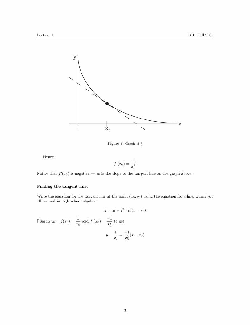
Figure 3: Graph of x 1

Hence,

f �(x0) = −

2

1x0

Notice that f �(x0) is negative — as is the slope of the tangent line on the graph above.

Finding the tangent line.

Write the equation for the tangent line at the point (x0, y0) using the equation for a line, which you all learned in high school algebra:

y − y0 = f �(x0)(x − x0)

Plug in y0 = f(x0) = 1

and f �(x0) = −

2

1 to get:

x0 x0

y − x

1

0 = −x2

0

1(x − x0)

3


y

xx0


Just for fun, let’s compute the area of the triangle that the tangent line forms with the x- and y-axes (see the shaded region in Fig. 4).

First calculate the x-intercept of this tangent line. The x-intercept is where y = 0. Plug y = 0 into the equation for this tangent line to get:

0 −1

= −

2

1(x − x0)

x0 x0

−1 −1 1 = x +2x0 x0 x0

1 2 x = 2x0 x0

2 x = x 20( ) = 2x0

x0

So, the x-intercept of this tangent line is at x = 2x0. 1 1

Next we claim that the y-intercept is at y = 2y0. Since y = and x = are identical equations, x y

the graph is symmetric when x and y are exchanged. By symmetry, then, the y-intercept is at y = 2y0. If you don’t trust reasoning with symmetry, you may follow the same chain of algebraic reasoning that we used in finding the x-intercept. (Remember, the y-intercept is where x = 0.)

Finally,1 1

Area = (2y0)(2x0) = 2x0y0 = 2x0( ) = 2 (see Fig. 5) 2 x0

Curiously, the area of the triangle is always 2, no matter where on the graph we draw the tangent line.

4


y

xx0 2x0

y0

2y0

x-1


Notations

Calculus, rather like English or any other language, was developed by several people. As a result, just as there are many ways to express the same thing, there are many notations for the derivative.

Since y = f(x), it’s natural to write

Δy = Δf = f(x) − f(x0) = f(x0 + Δx) − f(x0)

We say “Delta y” or “Delta f” or the “change in y”.

If we divide both sides by Δx = x − x0, we get two expressions for the difference quotient:

Δy =

Δf Δx Δx

Taking the limit as Δx → 0, we get

Δy Δx

→ dy dx

(Leibniz’ notation)

Δf Δx

→ f �(x0) (Newton’s notation)

When you use Leibniz’ notation, you have to remember where you’re evaluating the derivative — in the example above, at x = x0.

Other, equally valid notations for the derivative of a function f include

df , f �, and Df

dx

5


Example 2. f(x) = x n where n = 1, 2, 3...

dWhat is x n?

dx

To find it, plug y = f(x) into the definition of the difference quotient.

n nΔy =

(x0 + Δx)n − x0 =(x + Δx)n − x

Δx Δx Δx

(From here on, we replace x0 with x, so as to have less writing to do.) Since

(x + Δx)n = (x + Δx)(x + Δx)...(x + Δx) n times

We can rewrite this as � � x n + n(Δx)x n−1 + O (Δx)2

O(Δx)2 is shorthand for “all of the terms with (Δx)2, (Δx)3, and so on up to (Δx)n.” (This is part of what is known as the binomial theorem; see your textbook for details.)

n nΔy =

(x + Δx)n − x=

xn + n(Δx)(xn−1) + O(Δx)2 − x= nx n−1 + O(Δx)

Δx Δx Δx

Take the limit: Δy

lim = nx n−1

Δx 0 Δx→

Therefore,

d n x = nx n−1

dx

This result extends to polynomials. For example,

d 9(x 2 + 3x 10) = 2x + 30x dx

Physical Interpretation of Derivatives

You can think of the derivative as representing a rate of change (speed is one example of this).

On Halloween, MIT students have a tradition of dropping pumpkins from the roof of this building, which is about 400 feet high.

The equation of motion for objects near the earth’s surface (which we will just accept for now) implies that the height above the ground y of the pumpkin is:

y = 400 − 16t2

Δy distance travelled The average speed of the pumpkin (difference quotient) = =

Δt time elapsed

When the pumpkin hits the ground, y = 0,

400 − 16t2 = 0

6


Solve to find t = 5. Thus it takes 5 seconds for the pumpkin to reach the ground.

400 ft Average speed = = 80 ft/s

5 sec

A spectator is probably more interested in how fast the pumpkin is going when it slams into the ground. To find the instantaneous velocity at t = 5, let’s evaluate y�:

y� = −32t = (−32)(5) = −160 ft/s (about 110 mph)

y� is negative because the pumpkin’s y-coordinate is decreasing: it is moving downward.

7


Lecture 2: Limits, Continuity, and TrigonometricLimits

More about the “rate of change” interpretation of the derivative

y = f(x)y

x

∆x

∆y

Figure 1: Graph of a generic function, with Δx and Δy marked on the graph

3. T temperature gradient

Δy Δx

→ dy dx

as Δx → 0

Average rate of change → Instantaneous rate of change

Examples

1. q = charge dq dt

= electrical current

2. s = distance ds dt

= speed

dT = temperature =

dx

1


4. Sensitivity of measurements: An example is carried out on Problem Set 1. In GPS, radio signals give us h up to a certain measurement error (See Fig. 2 and Fig. 3). The question is

ΔLhow accurately can we measure L. To decide, we find . In other words, these variables are

Δh related to each other. We want to find how a change in one variable affects the other variable.

L

hs

satellite

you

Figure 2: The Global Positioning System Problem (GPS)

hs

L

Figure 3: On problem set 1, you will look at this simplified “flat earth” model

2

�


Limits and Continuity

Easy Limits

x2 + x 32 + 3 12lim = = = 3 x→3 x + 1 3 + 1 4

With an easy limit, you can get a meaningful answer just by plugging in the limiting value.

Remember,

lim Δf

= lim f(x0 + Δx) − f(x0)

x→x0 Δx x→x0 Δx

is never an easy limit, because the denominator Δx = 0 is not allowed. (The limit x x0 is computed under the implicit assumption that x =� x0.)

→

Continuity

We say f(x) is continuous at x0 when

lim f(x) = f(x0) x x0→

Pictures

x

y

Figure 4: Graph of the discontinuous function listed below

x + 1 x > 0 f(x) = −x x ≥ 0

3


This discontinuous function is seen in Fig. 4. For x > 0,

lim f(x) = 1x 0→

but f(0) = 0. (One can also say, f is continuous from the left at 0, not the right.)

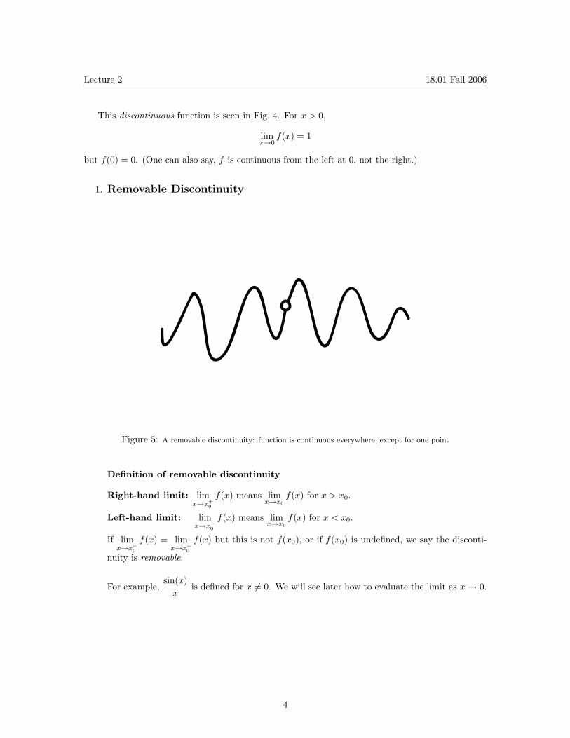
1. Removable Discontinuity

Figure 5: A removable discontinuity: function is continuous everywhere, except for one point

Definition of removable discontinuity

Right-hand limit: lim f(x) means lim f(x) for x > x0.+0

x x0→x x→

Left-hand limit: lim f(x) means lim f(x) for x < x0. 0x−

f(x) = lim f(x) but this is not f(x0), or if f(x0) is undefined, we say the disconti

x x0x →→

If lim +0 0x−→

nuity is removable. x x x→

For example, sin(

x

x) is defined for x = 0. We will see later how to evaluate the limit as � x → 0.

4


2. Jump Discontinuity

x0

Figure 6: An example of a jump discontinuity

lim for (x < x0) exists, and lim for (x > x0) also exists, but they are NOT equal.+0

−x0x x x→ →

3. Infinite Discontinuity

y

x

Figure 7: An example of an infinite discontinuity: 1

x

1 1Right-hand limit: lim = ∞; Left-hand limit: lim

x→0+ x x→0− x = −∞

5


4. Other (ugly) discontinuities

Figure 8: An example of an ugly discontinuity: a function that oscillates a lot as it approaches the origin

This function doesn’t even go to ±∞ — it doesn’t make sense to say it goes to anything. For something like this, we say the limit does not exist.

6


Picturing the derivative

x

y

xy’

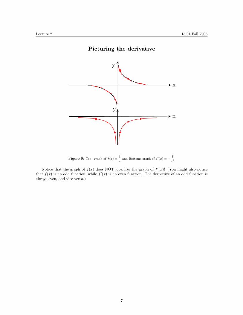
Figure 9: Top: graph of f (x) = 1

and Bottom: graph of f �(x) = − 12x x

Notice that the graph of f(x) does NOT look like the graph of f �(x)! (You might also notice that f(x) is an odd function, while f �(x) is an even function. The derivative of an odd function is always even, and vice versa.)

7


Pumpkin Drop, Part IIThis time, someone throws a pumpkin over the tallest building on campus.

Figure 10: y = 400 − 16t2 , −5 ≤ t ≤ 5

Figure 11: Top: graph of y(t) = 400 − 16t2 . Bottom: the derivative, y�(t)

8


Two Trig Limits

Note: In the expressions below, θ is in radians— NOT degrees!

lim sin θ

= 1; lim 1 − cos θ

= 0 θ 0 θ θ 0 θ→ →

Here is a geometric proof for the first limit:

1θ

arclength = θ

sinθ

Figure 12: A circle of radius 1 with an arc of angle θ

sin θ

arclength = θ

1θ

Figure 13: The sector in Fig. 12 as θ becomes very small

Imagine what happens to the picture as θ gets very small (see Fig. 13). As θ 0, we see that sin θ

→

1. θ

→

9


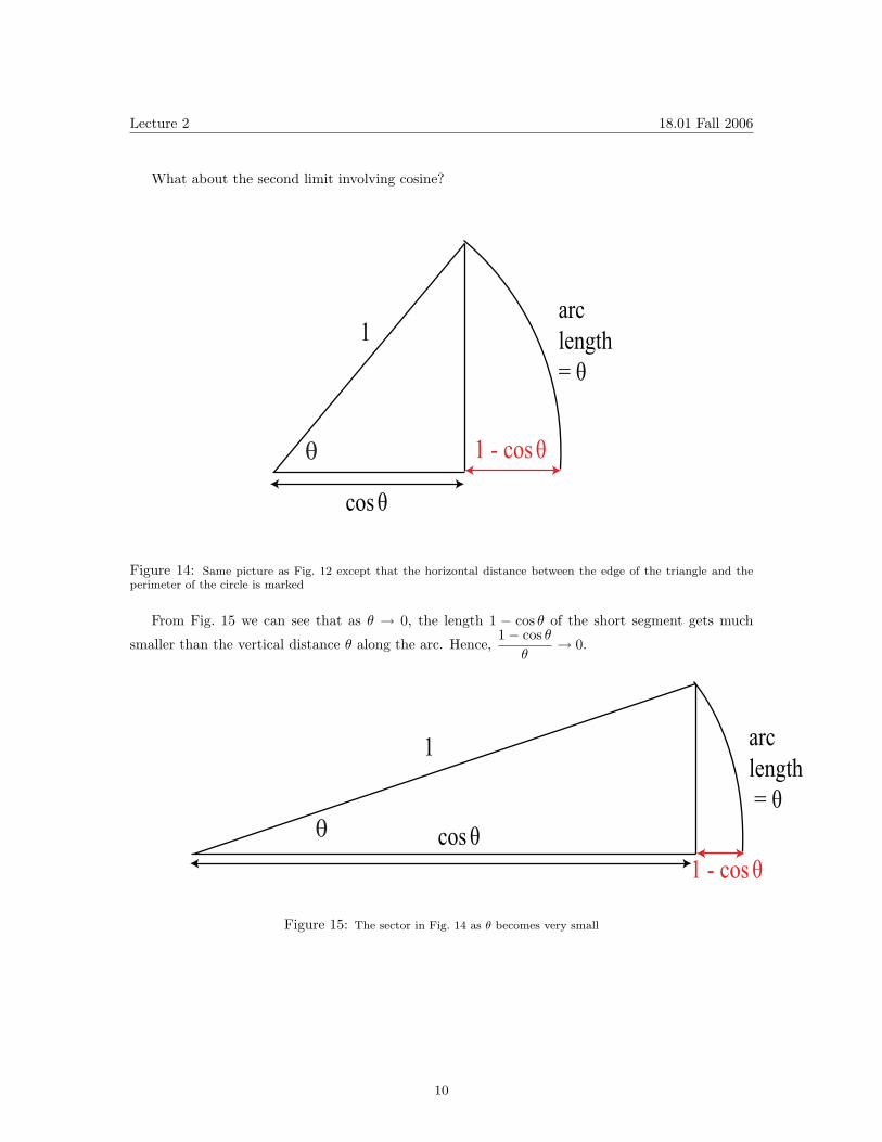
What about the second limit involving cosine?

1

cos θ

1 - cos θ

arclength = θ

θ

Figure 14: Same picture as Fig. 12 except that the horizontal distance between the edge of the triangle and the perimeter of the circle is marked

From Fig. 15 we can see that as θ → 0, the length 1 − cos θ of the short segment gets much

smaller than the vertical distance θ along the arc. Hence, 1 − cos θ

0. θ

→

1

cos θ1 - cos θ

arclength = θ

θ

Figure 15: The sector in Fig. 14 as θ becomes very small

10

� �


We end this lecture with a theorem that will help us to compute more derivatives next time.

Theorem: Differentiable Implies Continuous. If f is differentiable at x0, then f is continuous at x0.

f(x) − f(x0)Proof: xlim

x0

(f(x) − f(x0)) = xlim

x0 x − x0 (x − x0) = f �(x0) · 0 = 0.

→ →

Remember: you can never divide by zero! The first step was to multiply by x − x0 . It looks as

0 x − x0

if this is illegal because when x = x0, we are multiplying by . But when computing the limit as 0

x → x0 we always assume x �= x0. In other words x − x0 �= 0. So the proof is valid.

11

� �


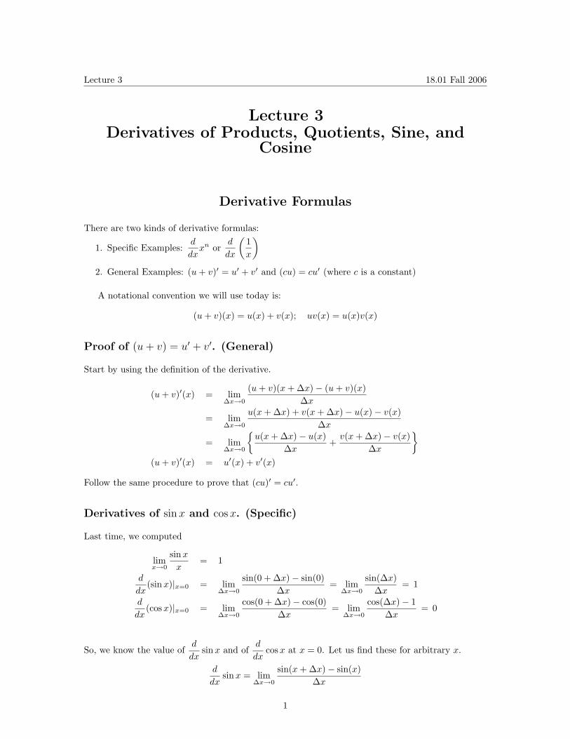
Lecture 3 Derivatives of Products, Quotients, Sine, and

Cosine

Derivative Formulas

There are two kinds of derivative formulas: d d 1

1. Specific Examples: x n or dx dx x

2. General Examples: (u + v)� = u� + v� and (cu) = cu� (where c is a constant)

A notational convention we will use today is:

(u + v)(x) = u(x) + v(x); uv(x) = u(x)v(x)

Proof of (u + v) = u� + v�. (General)

Start by using the definition of the derivative.

(u + v)�(x) = lim(u + v)(x + Δx) − (u + v)(x)

Δx 0 Δx→

= lim u(x + Δx) + v(x + Δx) − u(x) − v(x)

Δx 0 Δx→ � �

= lim u(x + Δx) − u(x)

+ v(x + Δx) − v(x)

Δx 0 Δx Δx→

(u + v)�(x) = u�(x) + v�(x)

Follow the same procedure to prove that (cu)� = cu�.

Derivatives of sin x and cos x. (Specific)

Last time, we computed

sin xlim = 1 x→0 x

d (sin x) x=0 = lim

sin(0 + Δx) − sin(0) = lim

sin(Δx)= 1

dx |

Δx→0 Δx Δx→0 Δx d

(cos x) x=0 = lim cos(0 + Δx) − cos(0)

= lim cos(Δx) − 1

= 0 dx

|Δx→0 Δx Δx→0 Δx

d dSo, we know the value of sin x and of cos x at x = 0. Let us find these for arbitrary x.

dx dx d

sin x = lim sin(x + Δx) − sin(x)

dx Δx 0 Δx→

1

� � � �


Recall:sin(a + b) = sin(a) cos(b) + sin(b) cos(a)

So,

d sin x = lim

sin x cos Δx + cos x sin Δx − sin(x) dx Δx 0 Δx→ � �

= lim sin x(cos Δx − 1)

+ cos x sin Δx

Δx 0 Δx Δx→ � � � �

= lim sin x cos Δx − 1

+ lim cos x sin Δx

Δx 0 Δx Δx 0 Δx→ →

Since cos Δx − 1

0 and that sin Δx

1, the equation above simplifies to Δx

→ Δx

→

d sin x = cos x

dx

A similar calculation gives d

cos x = − sin x dx

Product formula (General)

(uv)� = u�v + uv�

Proof:

(uv)� = lim (uv)(x + Δx) − (uv)(x)

= lim u(x + Δx)v(x + Δx) − u(x)v(x)


Now obviously, u(x + Δx)v(x) − u(x + Δx)v(x) = 0

so adding that to the numerator won’t change anything.

(uv)� = lim u(x + Δx)v(x) − u(x)v(x) + u(x + Δx)v(x + Δx) − u(x + Δx)v(x)

Δx 0 Δx→

We can re-arrange that expression to get

(uv)� = lim u(x + Δx) − u(x)

v(x) + u(x + Δx) v(x + Δx) − v(x)

Δx 0 Δx Δx→

Remember, the limit of a sum is the sum of the limits. � � � � ��

lim u(x + Δx) − u(x)

v(x) + lim u(x + Δx) v(x + Δx) − v(x)


(uv)� = u�(x)v(x) + u(x)v�(x)

Note: we also used the fact that

lim u(x + Δx) = u(x) (true because u is continuous) Δx 0→

This proof of the product rule assumes that u and v have derivatives, which implies both functions are continuous.

2


u ∆u

∆v

v

Figure 1: A graphical “proof” of the product rule

An intuitive justification:

We want to find the difference in area between the large rectangle and the smaller, inner rectangle. The inner (orange) rectangle has area uv. Define Δu, the change in u, by

Δu = u(x + Δx) − u(x)

We also abbreviate u = u(x), so that u(x + Δx) = u + Δu, and, similarly, v(x + Δx) = v + Δv. Therefore the area of the largest rectangle is (u + Δu)(v + Δv).

If you let v increase and keep u constant, you add the area shaded in red. If you let u increase and keep v constant, you add the area shaded in yellow. The sum of areas of the red and yellow rectangles is:

[u(v + Δv) − uv] + [v(u + Δu) − uv] = uΔv + vΔu

If Δu and Δv are small, then (Δu)(Δv) ≈ 0, that is, the area of the white rectangle is very small. Therefore the difference in area between the largest rectangle and the orange rectangle is approximately the same as the sum of areas of the red and yellow rectangles. Thus we have:

[(u + Δu)(v + Δv) − uv] ≈ uΔv + vΔu

(Divide by Δx and let Δx 0 to finish the argument.) →

3


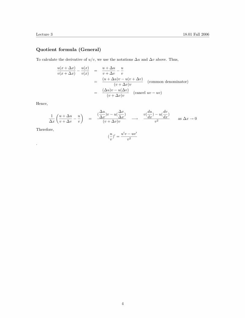
Quotient formula (General)

To calculate the derivative of u/v, we use the notations Δu and Δv above. Thus,

u(x + Δx) u(x)=

u + Δu u v(x + Δx)

− v(x) v + Δv

− v

=(u + Δu)v − u(v + Δv)

(common denominator) (v + Δv)v

= (Δu)v − u(Δv)

(v + Δv)v (cancel uv − uv)

Hence,

1 Δx

� u + Δu v + Δv

− u v

�

= ( Δu Δx

)v − u( Δv Δx

)

(v + Δv)v −→

v( du dx

) − u( dv dx

)

v2 as Δx → 0

Therefore,

( u v

)� = u�v − uv�

v2

.

4

Lecture 4 Sept. 14, 2006 18.01 Fall 2006

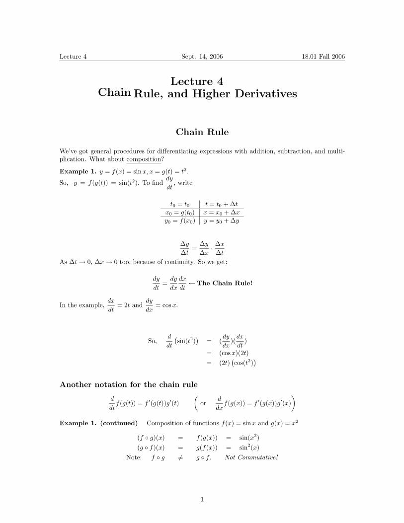
Lecture 4 Chain

Rule, and Higher Derivatives

Chain Rule

We’ve got general procedures for differentiating expressions with addition, subtraction, and multi plication. What about composition?

Example 1. y = f(x) = sin x, x = g(t) = t2 .

So, y = f(g(t)) = sin(t2). To find dy

, writedt

t = t0 + Δtt0 = t0

x = x0 + Δxx0 = g(t0) y = y0 + Δyy0 = f(x0)

Δy =

Δy Δx Δt Δx

· Δt

As Δt 0, Δx 0 too, because of continuity. So we get: → →

dy dy dx = The Chain Rule!

dt dx dt ←

In the example, dx dt

= 2t and dy dx

= cos x.

So, d dt

� sin(t2)

� = (

dy dx

)( dx dt

)

=

=

(cos x)(2t) (2t)

� cos(t2)

�

Another notation for the chain rule � � d dt

f(g(t)) = f �(g(t))g�(t) or d dx

f(g(x)) = f �(g(x))g�(x)

Example 1. (continued) Composition of functions f(x) = sin x and g(x) = x2

(f g)(x) = f(g(x)) = sin(x 2)◦ (g f)(x) = g(f(x)) = sin2(x)◦

Note: f ◦ g �= g ◦ f. Not Commutative!

1

� �

� � � �


x g g(x) f(g(x))f

Figure 1: Composition of functions: f g(x) = f(g(x))◦

d 1Example 2. cos = ?

dx x 1

Let u = x

dy =

dy du dx du dx dy du 1 du

= − sin(u); dx

= − x2 � �

1 � � sin dy sin(u) x

= = (− sin u) −1

= dx x2 x2 x2

d � � Example 3. x−n = ?

dx � �n1 1There are two ways to proceed. x−n = , or x−n =

x xn

1. d �

x−n �

= d

� 1 �n

= n

� 1 �n−1 �

−1 �

= −nx−(n−1)x−2 = −nx−n−1

dx dx x x x2

2. d �

x−n �

= d 1

= nx n−1 −1= −nx−n−1 (Think of xn as u)

dx dx xn x2n

2

� �


Higher Derivatives

Higher derivatives are derivatives of derivatives. For instance, if g = f �, then h = g� is the second derivative of f . We write h = (f �)� = f ��.

Notations

f �(x)

f ��(x)

f ��(x)

f (n)(x)

Df

D2f

D3f

Dnf

df dx

d2f dx2

d3f dx3

dnf dxn

Higher derivatives are pretty straightforward —- just keep taking the derivative!

nExample. Dnx = ?Start small and look for a pattern.

Dx = 1

D2 x 2 = D(2x) = 2 ( = 1 2)· D3 x 3 = D2(3x 2) = D(6x) = 6 (= 1 2 3)· · D4 x 4 = D3(4x 3) = D2(12x 2) = D(24x) = 24 (= 1 2 3 4)· · · Dn x n = n! we guess, based on the pattern we’re seeing here. ←

The notation n! is called “n factorial” and defined by n! = n(n − 1) 2 1· · · ·

Proof by Induction: We’ve already checked the base case (n = 1).

nInduction step: Suppose we know Dnx = n! (nth case). Show it holds for the (n + 1)st case.

Dn+1 x n+1 = Dn Dxn+1 = Dn ((n + 1)x n) = (n + 1)Dn x n = (n + 1)(n!)

Dn+1 x n+1 = (n + 1)!

Proved!

3

� �

� �

� �


Lecture 5 Implicit

Differentiation and Inverses

Implicit Differentiation

dExample 1. (x a) = ax a−1 .

dx We proved this by an explicit computation for a = 0, 1, 2, .... From this, we also got the formula for a = −1, −2, .... Let us try to extend this formula to cover rational numbers, as well:

m m

a = ; y = x n where m and n are integers. n

We want to compute dy

. We can say yn = xm so nyn−1 dy = mx m−1 . Solve for

dy :

dx dx dx

dy =

m xm−1

dx n yn−1

( m We know that y = x n ) is a function of x.

dy =

m xm−1

dx n yn−1

m xm−1

= n (xm/n)n−1

m xm−1

= n xm(n−1)/n

= x(m−1)− m(n

n −1)m

n m n(m−1)−m(n−1)

= x n n m nm−n−nm+m

= x n n m m n

= x n − n n

dy m m So, = x n − 1

dx n

This is the same answer as we were hoping to get!

Example 2. Equation of a circle with a radius of 1: x2 +y2 = 1 which we can write as y2 = 1−x2 . So y = ±

√1 − x2. Let us look at the positive case:

� 1y = + 1 − x2 = (1 − x 2) 2

dy =

1(1 − x 2)

−21 (−2x) =

−x = −x

dx 2 √

1 − x2 y

1


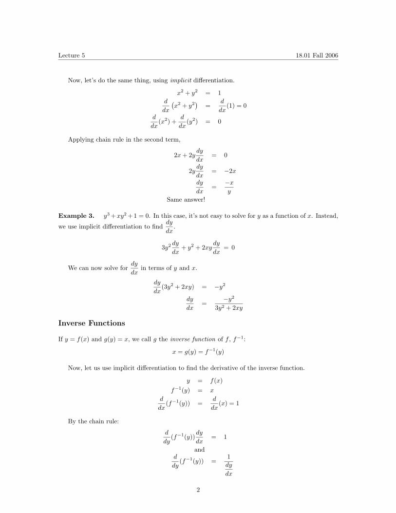
Now, let’s do the same thing, using implicit differentiation.

x 2 + y 2 = 1 d �

2� d

x 2 + y = (1) = 0 dx dx

d d(x 2) + (y 2) = 0

dx dx

Applying chain rule in the second term,

2x + 2ydy

= 0 dx

2ydy

= −2x dx dy

= −x

dx y Same answer!

Example 3. y3 + xy2 + 1 = 0. In this case, it’s not easy to solve for y as a function of x. Instead,

we use implicit differentiation to find dy

. dx

3y 2 dy + y 2 + 2xy

dy = 0

dx dx

We can now solve for dy

in terms of y and x. dx

dy dx

(3y 2 + 2xy) = −y 2

dy =

−y2

dx 3y2 + 2xy

Inverse Functions

If y = f(x) and g(y) = x, we call g the inverse function of f , f−1:

x = g(y) = f−1(y)

Now, let us use implicit differentiation to find the derivative of the inverse function.

y = f(x) f−1(y) = x

d d(f−1(y)) = (x) = 1

dx dx

By the chain rule:

d dy(f−1(y)) = 1

dy dx and

d 1(f−1(y)) =

dy dy dx

2

�


So, implicit differentiation makes it possible to find the derivative of the inverse function.

Example. y = arctan(x)

tan y = x d dx

[tan(y)] = dx dx

= 1

d dy

[tan(y)] � 1

cos2(y)

�

dy dx dy dx

=

=

1

1

dy dx

= cos2(y) = cos2(arctan(x))

This form is messy. Let us use some geometry to simplify it.

1

x

(1+x2)1/2y

Figure 1: Triangle with angles and lengths corresponding to those in the example illustrating differentiation using the inverse function arctan

In this triangle, tan(y) = x soarctan(x) = y

The Pythagorian theorem tells us the length of the hypotenuse:

h = 1 + x2

From this, we can find 1

cos(y) = √1 + x2

From this, we get � �21 1 cos2(y) = =√

1 + x2 1 + x2

3


So, dy

= 1

dx 1 + x2

In other words, d 1

arctan(x) = dx 1 + x2

Graphing an Inverse Function.

Suppose y = f(x) and g(y) = f−1(y) = x. To graph g and f together we need to write g as a function of the variable x. If g(x) = y, then x = f(y), and what we have done is to trade the variables x and y. This is illustrated in Fig. 2

f−1(f(x)) = x f−1 f(x) = x◦

f(f−1(x)) = x f f−1(x) = x◦

f(x)g(x)

a=f-1(b)

b=f(a)

x

y y=x

Figure 2: You can think about f −1 as the graph of f reflected about the line y = x

4

��


Lecture 6: Exponential and Log, Logarithmic Differentiation, Hyperbolic Functions

Taking the derivatives of exponentials and logarithms

Background

We always assume the base, a, is greater than 1.

a 0 = 1; a 1 = a; a 2 = a a; . . . ·

a x1+x2 = a x1 a x2

(a x1 )x2 = a x1 x2

p q

qa = √

ap (where p and q are integers)

rTo define a for real numbers r, fill in by continuity.

d Today’s main task: find a x

dx

We can write d ax+Δx x

x a = lim − a

dx Δx 0 Δx→

We can factor out the a x:x+Δx x Δx Δx

lim a − a

= lim a x a − 1= a x lim

a − 1 Δx 0 Δx Δx 0 Δx Δx 0 Δx→ → →

Let’s call

M(a) ≡ lim aΔx − 1

Δx 0 Δx→

We don’t yet know what M(a) is, but we can say

d a x = M(a)a x

dx

Here are two ways to describe M(a):

d1. Analytically M(a) = a x at x = 0.

dx

Indeed, M(a) = lim a0+Δx − a0

= d

a x

Δx 0 Δx dx→x=0

1


M(a) (slope of ax at x=0)

ax

Figure 1: Geometric definition of M(a)

x2. Geometrically, M(a) is the slope of the graph y = a at x = 0.

The trick to figuring out what M(a) is is to beg the question and define e as the number such that M(e) = 1. Now can we be sure there is such a number e? First notice that as the base a

xincreases, the graph a gets steeper. Next, we will estimate the slope M(a) for a = 2 and a = 4 geometrically. Look at the graph of 2x in Fig. 2. The secant line from (0, 1) to (1, 2) of the graph y = 2x has slope 1. Therefore, the slope of y = 2x at x = 0 is less: M(2) < 1 (see Fig. 2).

1 1Next, look at the graph of 4x in Fig. 3. The secant line from (−

2 , 2) to (1, 0) on the graph of

y = 4x has slope 1. Therefore, the slope of y = 4x at x = 0 is greater than M(4) > 1 (see Fig. 3).

Somewhere in between 2 and 4 there is a base whose slope at x = 0 is 1.

2


y=2x

slope M(2)

slope = 1 (1,2)

secant lin

e

Figure 2: Slope M(2) < 1

y=4x

secant line

(1,0)(-1/2, 1/2)

slope M(4)

Figure 3: Slope M(4) > 1

3


Thus we can define e to be the unique number such that

M(e) = 1

or, to put it another way,

lim eh − 1

= 1 h 0 h→

or, to put it still another way, d

(e x) = 1 at x = 0 dx

d dWhat is (e x)? We just defined M(e) = 1, and (e x) = M(e)e x . So

dx dx

d (e x) = e x

dx

Natural log (inverse function of ex)

To understand M(a) better, we study the natural log function ln(x). This function is defined as follows:

If y = e x , then ln(y) = x

(or)

If w = ln(x), then e x = w

xNote that e is always positive, even if x is negative. Recall that ln(1) = 0; ln(x) < 0 for 0 < x < 1; ln(x) > 0 for x > 1. Recall also that

ln(x1x2) = ln x1 + ln x2

Let us use implicit differentiation to find d

ln(x). w = ln(x). We want to find dw

. dx dx

e w = x d

(e w) = d

(x)dx dx

d (e w)

dw = 1

dw dx

e w dw = 1

dx dw 1 1

= = dx ew x

d 1(ln(x)) =

dx x

4


d Finally, what about (a x)?

dx

There are two methods we can use:

Method 1: Write base e and use chain rule.

Rewrite a as eln(a). Then, � �x a x = eln(a) = e x ln(a)

That looks like it might be tricky to differentiate. Let’s work up to it:

d e x = e x

dx and by the chain rule,

d e 3x = 3e 3x

dx

Remember, ln(a) is just a constant number– not a variable! Therefore,

de(ln a)x = (ln a)e(ln a)x

dx or

d (a x) = ln(a) a x

dx ·

Recall that d

(a x) = M (a) a x

dx ·

So now we know the value of M(a): M(a) = ln(a).

Even if we insist on starting with another base, like 10, the natural logarithm appears:

d 10x = (ln 10)10x

dx

The base e may seem strange at first. But, it comes up everywhere. After a while, you’ll learn to appreciate just how natural it is.

Method 2: Logarithmic Differentiation.

d dThe idea is to find f(x) by finding ln(f(x)) instead. Sometimes this approach is easier. Let

dx dx u = f(x). � �

d d ln(u) du 1 duln(u) = =

dx du dx u dx

duSince u = f and = f �, we can also write

dx

f �(ln f)� = or f � = f(ln f)�

f

5

� �

� �


xApply this to f(x) = a .

d d dln f(x) = x ln a = ln(f) = ln(a x) = (x ln(a)) = ln(a).⇒

dx dx dx

(Remember, ln(a) is a constant, not a variable.) Hence,

d f � d x x(ln f) = ln(a) = = ln(a) = f � = ln(a)f = a = (ln a)a dx

⇒ f

⇒ ⇒ dx

dExample 1. (x x) = ?

dx

With variable (“moving”) exponents, you should use either base e or logarithmic differentiation. In this example, we will use the latter.

f = x x

ln f = x ln x 1

(ln f)� = 1 (ln x) + x = ln(x) + 1 · x

f �(ln f)� =

f

Therefore, f � = f(ln f)� = x x (ln(x) + 1)

If you wanted to solve this using the base e approach, you would say f = ex ln x and differentiate it using the chain rule. It gets you the same answer, but requires a little more writing.

� �k1Example 2. Use logs to evaluate lim 1 + .

k→∞ k

Because the exponent k changes, it is better to find the limit of the logarithm.

�� k �

1lim ln 1 +

k→∞ k

We know that �� k � � �

1 1ln 1 + = k ln 1 +

k k

1This expression has two competing parts, which balance: k →∞ while ln 1 +

k → 0.

�� 1 �k

� � 1 �

ln � 1 + k

1 �

ln(1 + h) 1ln 1 + = k ln 1 + = 1 = (with h = )

k k h kk

Next, because ln 1 = 0 �� k �

ln 1 + 1

=ln(1 + h) − ln(1)

k h

6


1Take the limit: h =

k → 0 as k →∞, so that

ln(1 + h) − ln(1) d �� lim = ln(x)� = 1 h 0 h dx x=1→

In all, � �k1lim ln 1 + = 1.

k→∞ k � �k1We have just found that ak = ln[ 1 +

k ] → 1 as k →∞. � �k1

If bk = 1 + k

, then bk = e ak → e 1 as k → ∞. In other words, we have evaluated the limit we

wanted:

� �k1lim 1 + = e

k→∞ k

Remark 1. We never figured out what the exact numerical value of e was. Now we can use this limit formula; k = 10 gives a pretty good approximation to the actual value of e.

Remark 2. Logs are used in all sciences and even in finance. Think about the stock market. If I say the market fell 50 points today, you’d need to know whether the market average before the drop was 300 points or 10, 000. In other words, you care about the percent change, or the ratio of the change to the starting value:

f �(t) d = ln(f(t))

f(t) dt

7

� �


Lecture 7: Continuation and Exam Review

Hyperbolic Sine and Cosine

Hyperbolic sine (pronounced “sinsh”):

sinh(x) = ex − e−x

2

Hyperbolic cosine (pronounced “cosh”):

ex + e−x

cosh(x) = 2

x xd sinh(x) =

d e − e−x

= e − (−e−x)

= cosh(x)dx dx 2 2

Likewise, d

cosh(x) = sinh(x)dx

d(Note that this is different from cos(x).)

dx Important identity:

cosh2(x) − sinh2(x) = 1

Proof: � �2 � x �2

cosh2(x) − sinh2(x) = ex +

2 e−x

− e −

2 e−x

1 � � 1 � � 1cosh2(x) − sinh2(x) =

4 e 2x + 2e x e−x + e−2x −

4 e 2x − 2 + e−2x =

4(2 + 2) = 1

Why are these functions called “hyperbolic”? Let u = cosh(x) and v = sinh(x), then

u 2 − v 2 = 1

which is the equation of a hyperbola.

Regular trig functions are “circular” functions. If u = cos(x) and v = sin(x), then

u 2 + v 2 = 1

which is the equation of a circle.

1

� �

� �


Exam 1 Review

General Differentiation Formulas

(u + v)� = u� + v�

(cu)� = cu�

(uv)� = u�v + uv� (product rule) u �

= u�v − uv�

(quotient rule) v v2

d f(u(x)) = f �(u(x)) u�(x) (chain rule)

dx ·

You can remember the quotient rule by rewriting

u � = (uv−1)�

v

and applying the product rule and chain rule.

Implicit differentiation

Let’s say you want to find y� from an equation like

y 3 + 3xy 2 = 8

dInstead of solving for y and then taking its derivative, just take of the whole thing. In this

dx example,

3y 2 y� + 6xyy� + 3y 2 = 0

(3y 2 + 6xy)y� = −3y 2

y� = −3y2

3y2 + 6xy

Note that this formula for y� involves both x and y. Implicit differentiation can be very useful for taking the derivatives of inverse functions.

For instance,y = sin−1 x sin y = x⇒

Implicit differentiation yields (cos y)y� = 1

and 1 1

y� = = cos y

√1 − x2

2

� �


Specific differentiation formulas

You will be responsible for knowing formulas for the derivatives and how to deduce these formulas n xfrom previous information: x , sin−1 x, tan−1 x, sin x, cos x, tan x, sec x, e , ln x .

dFor example, let’s calculate sec x:

dx

d d 1 −(− sin x)sec x = = = tan x sec x

dx dx cos x cos2 x

d dYou may be asked to find sin x or cos x, using the following information:

dx dx

sin(h)lim = 1 h 0 h→

lim cos(h) − 1

= 0 h 0 h→

Remember the definition of the derivative:

df(x) = lim

f(x + Δx) − f(x) dx Δx 0 Δx→

Tying up a loose end

dHow to find x r, where r is a real (but not necessarily rational) number? All we have done so far

dx is the case of rational numbers, using implicit differentiation. We can do this two ways:

1st method: base e

x = e ln x

x r = � e ln x

�r = e r ln x

d dx

x r = d dx

e r ln x = e r ln x d dx

(r ln x) = e r ln x r x

d dx

x r = x r � r

x

� = rx r−1

2nd method: logarithmic differentiation

f �(ln f)� =

f f = x r

ln f = r ln x r

(ln f)� = x

f � = f(ln f)� = x r r = rx r−1

x

3

� � ��


Finally, in the first lecture I promised you that you’d learn to differentiate anything— even something as complicated as

d x tan−1 x e dx

So let’s do it!

d d e uv = e uv (uv) = e uv (u�v + uv�)

dx dx Substituting,

de x tan−1 x = e x tan−1 x tan−1 x + x

1 dx 1 + x2

4

18.01 single variable calculus fall 2006 for information ... · 2y 0 x-1 figure 15: graph of x ......

Documents