161 force control 7. force control -...

161

Force Control7. Force Control

Luigi Villani, Joris De Schutter

A fundamental requirement for the success ofa manipulation task is the capability to han-dle the physical contact between a robot andthe environment. Pure motion control turnsout to be inadequate because the unavoid-able modeling errors and uncertainties maycause a rise of the contact force, ultimatelyleading to an unstable behavior during the in-teraction, especially in the presence of rigidenvironments. Force feedback and force con-trol becomes mandatory to achieve a robustand versatile behavior of a robotic system inpoorly structured environments as well as safeand dependable operation in the presence ofhumans. This chapter starts from the analysisof indirect force control strategies, conceivedto keep the contact forces limited by ensuringa suitable compliant behavior to the end effec-tor, without requiring an accurate model of theenvironment. Then the problem of interactiontasks modeling is analyzed, considering boththe case of a rigid environment and the case ofa compliant environment. For the specificationof an interaction task, natural constraints setby the task geometry and artificial constraintsset by the control strategy are established, withrespect to suitable task frames. This formula-

7.1 Background ......................................... 1617.1.1 From Motion Control

to Interaction Control ................... 1617.1.2 From Indirect Force Control

to Hybrid Force/Motion Control ...... 163

7.2 Indirect Force Control............................ 1647.2.1 Stiffness Control ........................... 1647.2.2 Impedance Control ....................... 167

7.3 Interaction Tasks .................................. 1717.3.1 Rigid Environment ....................... 1717.3.2 Compliant Environment ................ 1737.3.3 Task Specification ......................... 1747.3.4 Sensor-Based Contact

Model Estimation ......................... 176

7.4 Hybrid Force/Motion Control .................. 1777.4.1 Acceleration-Resolved Approach .... 1777.4.2 Passivity-Based Approach ............. 1797.4.3 Velocity-Resolved Approach .......... 181

7.5 Conclusions and Further Reading ........... 1817.5.1 Indirect Force Control ................... 1827.5.2 Task Specification ......................... 1827.5.3 Hybrid Force/Motion Control .......... 182

References .................................................. 183

tion is the essential premise to the synthesis ofhybrid force/motion control schemes.

7.1 Background

Research on robot force control has flourished in thepast three decades. Such a wide interest is motivatedby the general desire of providing robotic systemswith enhanced sensory capabilities. Robots using force,touch, distance, and visual feedback are expected to au-tonomously operate in unstructured environments otherthan the typical industrial shop floor.

Since the early work on telemanipulation, the use offorce feedback was conceived to assist the human op-

erator in the remote handling of objects with a slavemanipulator. More recently, cooperative robot systemshave been developed where two or more manipulators(viz. the fingers of a dexterous robot hand) are to becontrolled so as to limit the exchanged forces and avoidsqueezing of a commonly held object. Force controlplays a fundamental role also in the achievement ofrobust and versatile behavior of robotic systems in open-ended environments, providing intelligent response in

PartA

7

162 Part A Robotics Foundations

unforeseen situations and enhancing human–robot in-teraction.

7.1.1 From Motion Controlto Interaction Control

Control of the physical interaction between a robotmanipulator and the environment is crucial for the suc-cessful execution of a number of practical tasks wherethe robot end-effector has to manipulate an object or per-form some operation on a surface. Typical examples inindustrial settings include polishing, deburring, machin-ing or assembly. A complete classification of possiblerobot tasks, considering also nonindustrial applications,is practically infeasible in view of the large variety ofcases that may occur, nor would such a classificationbe really useful to find a general strategy to control theinteraction with the environment.

During contact, the environment may set constraintson the geometric paths that can be followed by theend-effector, denoted as kinematic constraints. This sit-uation, corresponding to the contact with a stiff surface,is generally referred to as constrained motion. In othercases, the contact task is characterized by a dynamic in-teraction between the robot and the environment that canbe inertial (as in pushing a block), dissipative (as in slid-ing on a surface with friction) or elastic (as in pushingagainst an elastically compliant wall). In all these cases,the use of a pure motion control strategy for controllinginteraction is prone to failure, as explained below.

Successful execution of an interaction task with theenvironment by using motion control could be obtainedonly if the task were accurately planned. This would inturn require an accurate model of both the robot manipu-lator (kinematics and dynamics) and the environment(geometry and mechanical features). A manipulatormodel may be known with sufficient precision, buta detailed description of the environment is difficult toobtain.

To understand the importance of task planning ac-curacy, it is sufficient to observe that in order to performa mechanical part mating with a positional approach therelative positioning of the parts should be guaranteedwith an accuracy of an order of magnitude greater thanpart mechanical tolerance. Once the absolute position ofone part is exactly known, the manipulator should guidethe motion of the other with the same accuracy.

In practice, the planning errors may give rise toa contact force and moment, causing a deviation of theend-effector from the desired trajectory. On the otherhand, the control system reacts to reduce such devia-

tions. This ultimately leads to a build-up of the contactforce until saturation of the joint actuators is reached orbreakage of the parts in contact occurs.

The higher the environment stiffness and positioncontrol accuracy are, the more easily a situation likethe one just described can occur. This drawback can beovercome if a compliant behavior is ensured during theinteraction. This compliant behavior can be achievedeither in a passive or in an active fashion.

Passive Interaction ControlIn passive interaction control the trajectory of the robotend-effector is modified by the interaction forces dueto the inherent compliance of the robot. The compli-ance may be due to the structural compliance of thelinks, joints, and end-effector, or to the compliance ofthe position servo. Soft robot arms with elastic jointsor links are purposely designed for intrinsically safeinteraction with humans. In industrial applications, a me-chanical device with passive compliance, known as theremote center of compliance (RCC) device [7.1], iswidely adopted. An RCC is a compliant end-effectormounted on a rigid robot, designed and optimized forpeg-into-hole assembly operations.

The passive approach to interaction control isvery simple and cheap, because it does not requireforce/torque sensors; also, the preprogrammed trajec-tory of the end-effector must not be changed at executiontime; moreover, the response of a passive compliancemechanism is much faster than active repositioningby a computer control algorithm. However, the use ofpassive compliance in industrial applications lacks flex-ibility, since for every robotic task a special-purposecompliant end-effector has to be designed and mounted.Also, it can only deal with small position and orientationdeviations of the programmed trajectory. Finally, sinceno forces are measured, it can not guarantee that highcontact forces will never occur.

Active Interaction ControlIn active interaction control, the compliance of therobotic system is mainly ensured by a purposely de-signed control system. This approach usually requiresthe measurement of the contact force and moment,which are fed back to the controller and used to mod-ify or even generate online the desired trajectory of therobot end-effector.

Active interaction control may overcome the afore-mentioned disadvantages of passive interaction control,but it is usually slower, more expensive, and more so-phisticated. To obtain a reasonable task execution speed

PartA

7.1

Force Control 7.1 Background 163

and disturbance rejection capability, active interactioncontrol has to be used in combination with some degreeof passive compliance [7.2]: feedback, by definition, al-ways comes after a motion and force error has occurred,hence some passive compliance is needed in order tokeep the reaction forces below an acceptable threshold.

Force MeasurementsFor a general force-controlled task, six force compo-nents are required to provide complete contact forceinformation: three translational force components andthree torques. Often, a force/torque sensor is mountedat the robot wrist [7.3], but other possibilities exist, forexample, force sensors can be placed on the fingertipsof robotic hands [7.4]; also, external forces and mo-ments can be estimated via shaft torque measurementsof joint torque sensors [7.5, 6]. However, the majorityof the applications of force control (including indus-trial applications) is concerned with wrist force/torquesensors. In this case, the weight and inertia of the toolmounted between the sensor and the environment (i. e.,the robot end-effector) is assumed to be negligible orsuitably compensated from the force/torque measure-ments. The force signals may be obtained using strainmeasurements, which results in a stiff sensor, or de-formation measurements (e.g., optically), resulting ina compliant sensor. The latter approach has an advantageif additional passive compliance is desired.

7.1.2 From Indirect Force Controlto Hybrid Force/Motion Control

Active interaction control strategies can be grouped intotwo categories: those performing indirect force controland those performing direct force control. The maindifference between the two categories is that the for-mer achieve force control via motion control, withoutexplicit closure of a force feedback loop; the latter in-stead offer the possibility of controlling the contact forceand moment to a desired value, thanks to the closure ofa force feedback loop.

To the first category belongs impedance control (oradmittance control) [7.7, 8], where the deviation of theend-effector motion from the desired motion due to theinteraction with the environment is related to the con-tact force through a mechanical impedance/admittancewith adjustable parameters. A robot manipulator underimpedance (or admittance) control is described by anequivalent mass–spring–damper system with adjustableparameters. This relationship is an impedance if therobot control reacts to the motion deviation by gener-

ating forces, while it corresponds to an admittance if therobot control reacts to interaction forces by imposinga deviation from the desired motion. Special cases ofimpedance and admittance control are stiffness controland compliance control [7.9], respectively, where onlythe static relationship between the end-effector positionand orientation deviation from the desired motion andthe contact force and moment is considered. Notice that,in the robot control literature, the terms impedance con-trol and admittance control are often used to refer to thesame control scheme; the same happens for stiffness andcompliance control. Moreover, if only the relationshipbetween the contact force and moment and the end-effector linear and angular velocity is of interest, thecorresponding control scheme is referred to as dampingcontrol [7.10].

Indirect force control schemes do not require, inprinciple, measurements of contact forces and moments;the resulting impedance or admittance is typically non-linear and coupled. However, if a force/torque sensoris available, then force measurements can be used inthe control scheme to achieve a linear and decoupledbehavior.

Differently from indirect force control, direct forcecontrol requires an explicit model of the interactiontask. In fact, the user has to specify the desired motionand the desired contact force and moment in a con-sistent way with respect to the constraints imposedby the environment. A widely adopted strategy be-longing to this category is hybrid force/motion control,which aims at controlling the motion along the uncon-strained task directions and force (and moment) alongthe constrained task directions. The starting point isthe observation that, for many robotic tasks, it is pos-sible to introduce an orthogonal reference frame, knownas the compliance frame [7.11] (or task frame [7.12])which allows one to specify the task in terms of nat-ural and artificial constrains acting along and aboutthe three orthogonal axes of this frame. Based on thisdecomposition, hybrid force/motion control allows si-multaneous control of both the contact force and theend-effector motion in two mutually independent sub-spaces. Simple selection matrices acting on both thedesired and feedback quantities serve this purpose forplanar contact surfaces [7.13], whereas suitable projec-tion matrices must be used for general contact tasks,which can also be derived from the explicit constraintequations [7.14–16]. Several implementation of hybridmotion control schemes are available, e.g., based on in-verse dynamics control in the operational space [7.17],passivity-based control [7.18], or outer force control

PartA

7.1


loops closed around inner motion loops, typically avail-able in industrial robots [7.2].

If an accurate model of the environment is notavailable, the force control action and the motion con-trol action can be superimposed, resulting in a parallel

force/position control scheme. In this approach, the forcecontroller is designed so as to dominate the motion con-troller; hence, a position error would be tolerated alongthe constrained task directions in order to ensure forceregulation [7.19].

7.2 Indirect Force Control

To gain insight into the problems arising at the inter-action between the end-effector of a robot manipulatorand the environment, it is worth analyzing the effects ofa motion control strategy in the presence of a contactforce and moment. To this aim, assume that a refer-ence frame Σe is attached to the end-effector, and letpe denote the position vector of the origin and Re therotation matrix with respect to a fixed base frame. Theend-effector velocity is denoted by the 6 × 1 twist vec-tor ve = (

p�e ω�

e

)� where pe is the translational velocityand ωe the angular velocity, and can be computed fromthe n × 1 joint velocity vector q using the linear mapping

ve = J(q)q . (7.1)

The matrix J is the 6 × n end-effector geometricJacobian. For simplicity, the case of nonredundant non-singular manipulators is considered; therefore, n = 6and the Jacobian is a square nonsingular matrix. Theforce f e and moment me applied by the end-effectorto the environment are the components of the wrenchhe = (

f �e m�

e

)�.It is useful to consider the operational space formu-

lation of the dynamic model of a rigid robot manipulatorin contact with the environment

Λ(q)ve +Γ (q, q)ve +η(q) = hc −he , (7.2)

where Λ(q) = (JH(q)−1 J�)−1 is the 6 × 6 operatio-nal space inertia matrix, Γ (q, q) = J−�C(q, q)J−1 −Λ(q) J J−1 is the wrench including centrifugal andCoriolis effects, and η(q) = J−�g(q) is the wrench ofthe gravitational effects; H(q), C(q, q) and g(q) are thecorresponding quantities defined in the joint space. Thevector hc = J−�τ is the equivalent end-effector wrenchcorresponding to the input joint torques τ.

7.2.1 Stiffness Control

In the classical operational space formulation, the end-effector position and orientation is described by a 6 × 1vector xe = (

p�e ϕ�

e

)�, where ϕe is a set of Euler angles

extracted from Re. Hence, a desired end-effector posi-tion and orientation can be assigned in terms of a vectorxd, corresponding to the position of the origin pd andthe rotation matrix Rd of a desired frame Σd. The end-effector error can be denoted as Δxde = xd − xe, and thecorresponding velocity error, assuming a constant xd,can be expressed as Δxde = −xe = −A−1(ϕe)ve, with

A(ϕe) =(

I 00 T(ϕe)

)

,

where I is the 3 × 3 identity matrix, 0 is a 3 × 3 nullmatrix, and T is the 3 × 3 matrix of the mappingωe = T(ϕe)ϕe, depending on the particular choice of

the Euler angles.Consider the motion control law

hc = A−�(ϕe)KPΔxde − KDve +η(q) , (7.3)

corresponding to a simple PD + gravity compensationcontrol in the operational space, where KP and KD aresymmetric and positive-definite 6 × 6 matrices.

In the absence of interaction with the environment(i. e., when he = 0), the equilibrium ve = 0, Δxde = 0for the closed-loop system, corresponding to the de-sired position and orientation for the end-effector, isasymptotically stable. The stability proof is based onthe positive-definite Lyapunov function

V = 1

2v�

e Λ(q)ve + 1

2Δxde KPΔxde ,

whose time derivative along the trajectories of theclosed-loop system is the negative semidefinite function

V = −v�e KDve . (7.4)

In the presence of a constant wrench he, using a similarLyapunov argument, a different asymptotically stableequilibrium can be found, with a nonnull Δxde. Thenew equilibrium is the solution of the equation

A−�(ϕe)KPΔxde −he = 0 ,

which can be written in the form

Δxde = K−1P A�(ϕe)he , (7.5)

PartA

7.2

Force Control 7.2 Indirect Force Control 165

or, equivalently, as

he = A−�(ϕe)KPΔxde . (7.6)

Equation (7.6) shows that in the steady state the end-effector, under a proportional control action on theposition and orientation error, behaves as a six-degree-of-freedom (DOF) spring in respect of the external forceand moment he. Thus, the matrix KP plays the roleof an active stiffness, eaning that it is possible to acton the elements of KP so as to ensure a suitable elas-tic behavior of the end-effector during the interaction.Analogously, (7.5) represents a compliance relationship,where the matrix K−1

P plays the role of an active compli-ance. This approach, consisting of assigning a desiredposition and orientation and a suitable static relationshipbetween the deviation of the end-effector position andorientation from the desired motion and the force exertedon the environment, is known as stiffness control.

The selection of the stiffness/compliance parametersis not easy, and strongly depends on the task to be ex-ecuted. A higher value of the active stiffness meansa higher accuracy of the position control at the expense ofhigher interaction forces. Hence, if it is expected to meetsome physical constraint in a particular direction, theend-effector stiffness in that direction should be madelow to ensure low interaction forces. Conversely, alongthe directions where physical constraints are not ex-pected, the end-effector stiffness should be made highso as to follow closely the desired position. This al-lows discrepancies between the desired and achievablepositions due to the constraints imposed by the environ-ment to be resolved without excessive contact forces andmoments.

It must be pointed out, however, that a selectivestiffness behavior along different directions cannot beeffectively assigned in practice on the basis of (7.6). Thiscan easily be understood by using the classical definitionof a mechanical stiffness for two bodies connected bya 6-DOF spring, in terms of the linear mapping betweenthe infinitesimal twist displacement of the two bodies atan unloaded equilibrium and the elastic wrench.

In the case of the active stiffness, the two bodies are,respectively, the end-effector, with the attached frameΣe, and a virtual body, attached to the desired frameΣd. Hence, from (7.6), the following mapping can bederived

he = A−�(ϕe)KP A−1(ϕe)δxde , (7.7)

in the case of an infinitesimal twist displacement δxdedefined as

δxde =(

δpde

δθde

)

=(

Δ pde

Δωde

)

dt = −(

pe

ωe

)

dt ,

where Δ pde = pd − pe is the time derivative of the po-sition error Δpde = pd − pe and Δωde = ωd −ωe is theangular velocity error. Equation (7.7) shows that theactual stiffness matrix is A−�(ϕe)KP A−1(ϕe), whichdepends on the end-effector orientation through the vec-tor ϕe, so that, in practice, the selection of the stiffnessparameters is quite difficult.

This problem can be overcome by defining a geomet-rically consistent active stiffness, with the same structureand properties as ideal mechanical springs.

Mechanical SpringsConsider two elastically coupled rigid bodies A and Band two reference frames Σa and Σb, attached to A andB, respectively. Assuming that at equilibrium framesΣa and Σb coincide, the compliant behavior near theequilibrium can be described by the linear mapping

hbb = Kδxb

ab =(

K t K c

K�c Ko

)

δxbab , (7.8)

where hbb is the elastic wrench applied to body B, ex-

pressed in frame B, in the presence of an infinitesimaltwist displacement δxb

ab of frame Σa with respect toframe Σb, expressed in frame B. The elastic wrenchand the infinitesimal twist displacement in (7.8) canalso be expressed equivalently in frame Σa, since Σaand Σb coincide at equilibrium. Therefore, hb

b = hab and

δxbab = δxa

ab; moreover, for the elastic wrench applied tobody A, ha

a = K tδxaba = −hb

b being δxaba = −δxb

ab. Thisproperty of the mapping (7.8) is known as port symmetry.

In (7.8), K is the 6 × 6 symmetric positive-semidefinite stiffness matrix. The 3 × 3 matrices K t andKo, called respectively the translational stiffness and ro-tational stiffness, are also symmetric. It can be shownthat, if the 3 × 3 matrix K c, called the coupling stiffnessis symmetric, there is maximum decoupling betweenrotation and translation. In this case, the point corres-ponding to the coinciding origins of the frames Σa andΣb is called the center of stiffness. Similar definitionsand results can be formulated for the case of the com-pliance matrix C = K−1. In particular, it is possible todefine a center of compliance in the case that the off-diagonal blocks of the compliance matrix are symmetric.The center of stiffness and compliance do not necessarilycoincide.

There are special cases in which no coupling existsbetween translation and rotation, i. e., a relative transla-

PartA

7.2


tion of the bodies results in a wrench corresponding toa pure force along an axis through the center of stiff-ness; also, a relative rotation of the bodies results ina wrench that is equivalent to a pure torque about anaxis through the centers of stiffness. In these cases, thecenter of stiffness and compliance coincide. Mechanicalsystems with completely decoupled behavior are, e.g.,the remote center of compliance (RCC) devices.

Since K t is symmetric, there exists a rotation matrixRt with respect to the frame Σa = Σb at equilibrium,such that K t = Rt Γ t R�

t , and Γ t is a diagonal matrixwhose diagonal elements are the principal transla-tional stiffnessess in the directions corresponding to thecolumns of the rotation matrix Rt, known as the princi-pal axes of translational stiffness. Analogously, Ko canbe expressed as Ko = Ro Γ o R�

o , where the diagonalelements of Γ o are the principal rotational stiffnessesabout the axes corresponding to the columns of rotationmatrix Ro, known as the principal axes of rotationalstiffness. Moreover, assuming that the origins of Σa andΣb at equilibrium coincide with the center of stiffness,the expression K c = Rc Γ c R�

c can be found, where thediagonal elements of Γ c are the principal coupling stiff-nesses along the directions corresponding to the columnsof the rotation matrix Rc, known as the principal axesof coupling stiffness. In sum, a 6 × 6 stiffness matrix canbe specified, with respect to a frame with origin in thecenter of stiffness, in terms of the principal stiffnessparameters and principal axes.

Notice that the mechanical stiffness defined by (7.8)describes the behavior of an ideal 6-DOF spring whichstores potential energy. The potential energy function ofan ideal stiffness depends only on the relative positionand orientation of the two attached bodies and is portsymmetric. A physical 6-DOF spring has a predomi-nant behavior similar to the ideal one, but neverthelessit always has parasitic effects causing energy dissipa-tion.

Geometrically Consistent Active StiffnessTo achieve a geometrically consistent 6-DOF active stiff-ness, a suitable definition of the proportional controlaction in control law (7.3) is required. This control ac-tion can be interpreted as the elastic wrench applied tothe end-effector, in the presence of a finite displacementof the desired frame Σd with respect to the end-effectorframe Σe. Hence, the properties of the ideal mechanicalstiffness for small displacements should be extended tothe case of finite displacements. Moreover, to guaranteeasymptotic stability in the sense of Lyapunov, a suitablepotential elastic energy function must be defined.

For simplicity, it is assumed that the coupling stiff-ness matrix is zero. Hence, the potential elastic energycan be computed as the sum of a translational potentialenergy and a rotational potential energy.

The translational potential energy can be defined as

Vt = 1

2Δp�

de K ′PtΔpde (7.9)

with

K ′Pt = 1

2Rd KPt R�

d + 1

2Re KPt R�

e ,

where KPt is a 3 × 3 symmetric positive-definite matrix.The use of K ′

Pt in lieu of KPt in (7.9) guarantees thatthe potential energy is port symmetric also in the caseof finite displacements. Matrices K ′

Pt and KPt coincideat equilibrium (i. e., when Rd = Re) and in the case ofisotropic translational stiffness (i. e., when KPt = kPt I).

The computation of the power Vt yields

Vt = Δ pe�de f e

Δt +Δωe�de me

Δt ,

where Δ pede is the time derivative of the posi-

tion displacement Δpede = R�

e (pd − pe), while Δωede =

R�e (ωd −ωe). The vectors f e

Δ and μeΔ are, respectively,

the elastic force and moment applied to the end-effectorin the presence of the finite position displacement Δpe

de.These vectors have the following expressions whencomputed in the base frame

fΔt = K ′PtΔpde mΔt = K ′′

PtΔpde (7.10)

with

K ′′Pt = 1

2S(Δpde)Rd KPt R�

d ,

where S(·) is the skew-symmetric operator performingthe vector product. The vector hΔt = (

f �Δt m�

Δt

)� is theelastic wrench applied to the end-effector in the pres-ence of a finite position displacement Δpde and a nullorientation displacement. The moment mΔt is null in thecase of isotropic translational stiffness.

To define the rotational potential energy, a suitabledefinition of the orientation displacement between theframes Σd and Σe has to be adopted. A possible choiceis the vector part of the unit quaternion {ηde, ε

ede} that

can be extracted from matrix Red = R�

e Rd. Hence, theorientation potential energy has the form

Vo = 2εe�de KPoε

ede , (7.11)

where KPo is a 3 × 3 symmetric positive-definite matrix.The function Vo is port symmetric because εe

de = −εded.

PartA

7.2


The computation of the power Vo yields

Vo = Δωe�de me

Δo ,

where

mΔo = K ′Poεde , (7.12)

with

K ′Po = 2E�(ηde, εde)Re KPo R�

e

and E(ηde, εde) = ηde I − S(εde). The above equationsshow that a finite orientation displacement εde = R�

e εede

produces an elastic wrench hΔo = (0� m�Δo)� which is

equivalent to a pure moment.Hence, the total elastic wrench in the presence of

a finite position and orientation displacement of the de-sired frame Σd with respect to the end-effector frameΣe can be defined in the base frame as

hΔ = hΔt +hΔo . (7.13)

where hΔt and hΔo are computed according to (7.10)and (7.12), respectively.

Using (7.13) for the computation of the elasticwrench in the case of an infinitesimal twist displacementδxe

de near the equilibrium, and discarding the high-orderinfinitesimal terms, yields the linear mapping

hee = KPδxe

de =(

KPt 00 KPo

)

δxede . (7.14)

Therefore, KP represents the stiffness matrix of an idealspring with respect to a frame Σe (coinciding with Σdat equilibrium) with the origin at the center of stiff-ness. Moreover, it can be shown, using definition (7.13),that the physical/geometrical meaning of the principalstiffnesses and of the principal axes for the matricesKPt and KPo are preserved also in the case of largedisplacements.

The above results imply that the active stiffness ma-trix KP can be set in a geometrically consistent way withrespect to the task at hand.

Notice that geometrical consistency can also be en-sured with different definitions of the orientation errorin the potential orientation energy (7.11), for example,any error based on the angle/axis representation of Rd

ecan be adopted (the unit quaternion belongs to this cat-egory), or, more generally, homogeneous matrices orexponential coordinates (for the case of both positionand orientation errors). Also, the XYZ Euler angles ex-tracted from the matrix Rd

e could be used; however, inthis case, it can be shown that the principal axes of rota-tional stiffness cannot be set arbitrarily but must coincidewith those of the end-effector frame.

Compliance control with a geometrically consistentactive stiffness can be defined using the control law

hc = hΔ − KDve +η(q) ,

with hΔ in (7.13). The asymptotic stability about theequilibrium in the case he = 0 can be proven using theLyapunov function

V = 1

2v�

e Λ(q)ve + Vt + Vo ,

with Vt and Vo given in (7.9) and (7.11), respectively,whose time derivative along the trajectories of theclosed-loop system, in case the frame Σd is motionless,has the same expression as in (7.4). When he �= 0, a dif-ferent asymptotically stable equilibrium can be found,corresponding to a nonnull displacement of the desiredframe Σd with respect to the end-effector frame Σe. Thenew equilibrium is the solution of the equation hΔ = he.

Stiffness control allows to keep the interaction forceand moment limited at the expense of the end-effectorposition and orientation error, with a proper choice ofthe stiffness matrix, without the need of a force/torquesensor. However, in the presence of disturbances (e.g.,joint friction) which can be modeled as an equivalentend-effector wrench, the adoption of low values for theactive stiffness may produce large deviations with re-spect to the desired end-effector position and orientation,also in the absence of interaction with the environment.

7.2.2 Impedance Control

Stiffness control is designed to achieve a desired staticbehavior of the interaction. In fact, the dynamics ofthe controlled system depends on that of the robotmanipulator, which is nonlinear and coupled. A moredemanding objective may be that of achieving a de-sired dynamic behavior for the end-effector, e.g., that ofa second-order mechanical system with six degrees offreedom, characterized by a given mass, damping, andstiffness, known as mechanical impedance.

The starting point to pursue this goal may be theacceleration-resolved approach used for motion con-trol, which is aimed at decoupling and linearizing thenonlinear robot dynamics at the acceleration level viaan inverse dynamics control law. In the presence ofinteraction with the environment, the control law

hc = Λ(q)α+Γ (q, q)q +he (7.15)

cast into the dynamic model (7.2) results in

ve = α , (7.16)

PartA

7.2


where α is a properly designed control input with themeaning of an acceleration referred to the base frame.Considering the identity ve = Re

�vee + ˙Re

�vee, with

Re =(

Re 00 Re

)

,

the choice

α = Re�αe + ˙R�

e vee (7.17)

gives

vee = αe , (7.18)

where the control input αe has the meaning of an ac-celeration referred to the end-effector frame Σe. Hence,setting

αe = K−1M (ve

d + KDΔvede +he

Δ −hee) , (7.19)

the following expression can be found for the closed-loop system

KMΔvede + KDΔve

de +heΔ = he

e , (7.20)

where KM and KD are 6 × 6 symmetric and positive-definite matrices, Δve

de = ved − ve

e, Δvede = ve

d −vee, ve

dand ve

d are, respectively, the acceleration and the vel-ocity of a desired frame Σd and he

Δ is the elasticwrench (7.13); all the quantities are referred to theend-effector frame Σe.

The above equation describing the dynamic behav-ior of the controlled end-effector can be interpreted asa generalized mechanical impedance. The asymptoticstability of the equilibrium in the case he = 0 can beproven by considering the Lyapunov function

V = 1

2Δve�

de KMΔvede + Vt + Vo , (7.21)

Directkinematics

Inversedynamics

Impedancecontrol

Manipulatorand

environment

α τhe

qq·

pd, Rd

υd

pe, Re

υe

υ·d

Fig. 7.1 Impedance control

where Vt and Vo are defined in (7.9) and (7.11), respec-tively, and whose time derivative along the trajectoriesof system (7.20) is the negative semidefinite function

V = −Δve�de KDΔve

de .

When he �= 0, a different asymptotically stable equi-librium can be found, corresponding to a nonnulldisplacement of the desired frame Σd with respect tothe end-effector frame Σe. The new equilibrium is thesolution of the equation he

Δ = he.In case Σd is constant, (7.20) has the meaning of

a true 6-DOF mechanical impedance if KM is chosen as

KM =(

m I 00 M

)

,

where m is a mass and M is a 3 × 3 inertia tensor,and KD is chosen as a block-diagonal matrix with 3 × 3blocks. The physically equivalent system is a body ofmass m with inertia tensor M with respect to a frameΣe attached to the body, subject to an external wrenchhe. This body is connected to a virtual body attached toframe Σd through a 6-DOF ideal spring with stiffnessmatrix KP and is subject to viscous forces and momentswith damping KD. The function V in (7.21) representsthe total energy of the body: the sum of the kinetic andpotential elastic energy.

A block diagram of the resulting impedance controlis sketched in Fig. 7.1. The impedance control computesthe acceleration input as in (7.17) and (7.19) on thebasis of the position and orientation feedback as wellas the force and moment measurements. Then, the in-verse dynamics control law computes the torques for thejoint actuators τ = J�hc with hc in (7.15). This controlscheme, in the absence of interaction, guarantees thatthe end-effector frame Σe asymptotically follows thedesired frame Σd. In the presence of contact with theenvironment, a compliant dynamic behavior is imposedon the end-effector, according to the impedance (7.20),and the contact wrench is bounded at the expense of a fi-nite position and orientation displacement between Σdand Σe. Differently from stiffness control, a force/torquesensor is required for the measurement of the contactforce and moment.

Implementation IssuesThe selection of good impedance parameters ensuringa satisfactory behavior is not an easy task. In fact, thedynamics of the closed-loop system is different in freespace and during interaction. The control objectives aredifferent as well, since motion tracking and disturbance

PartA

7.2


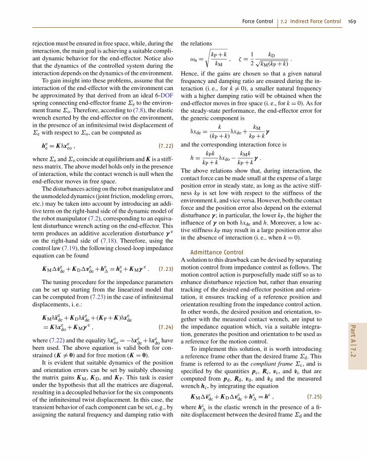
rejection must be ensured in free space, while, during theinteraction, the main goal is achieving a suitable compli-ant dynamic behavior for the end-effector. Notice alsothat the dynamics of the controlled system during theinteraction depends on the dynamics of the environment.

To gain insight into these problems, assume that theinteraction of the end-effector with the environment canbe approximated by that derived from an ideal 6-DOFspring connecting end-effector frame Σe to the environ-ment frame Σo. Therefore, according to (7.8), the elasticwrench exerted by the end-effector on the environment,in the presence of an infinitesimal twist displacement ofΣe with respect to Σo, can be computed as

hee = Kδxe

eo , (7.22)

where Σe and Σo coincide at equilibrium and K is a stiff-ness matrix. The above model holds only in the presenceof interaction, while the contact wrench is null when theend-effector moves in free space.

The disturbances acting on the robot manipulator andthe unmodeled dynamics (joint friction, modeling errors,etc.) may be taken into account by introducing an addi-tive term on the right-hand side of the dynamic model ofthe robot manipulator (7.2), corresponding to an equiva-lent disturbance wrench acting on the end-effector. Thisterm produces an additive acceleration disturbance γ e

on the right-hand side of (7.18). Therefore, using thecontrol law (7.19), the following closed-loop impedanceequation can be found

KMΔvede + KDΔve

de +heΔ = he

e + KMγ e . (7.23)

The tuning procedure for the impedance parameterscan be set up starting from the linearized model thatcan be computed from (7.23) in the case of infinitesimaldisplacements, i. e.:

KMδxede + KDδxe

de + (KP + K )δxede

= Kδxedo + KMγ e , (7.24)

where (7.22) and the equality δxeeo = −δxe

de +δxedo have

been used. The above equation is valid both for con-strained (K �= 0) and for free motion (K = 0).

It is evident that suitable dynamics of the positionand orientation errors can be set by suitably choosingthe matrix gains KM, KD, and KP. This task is easierunder the hypothesis that all the matrices are diagonal,resulting in a decoupled behavior for the six componentsof the infinitesimal twist displacement. In this case, thetransient behavior of each component can be set, e.g., byassigning the natural frequency and damping ratio with

the relations

ωn =√

kP + k

kM, ζ = 1

2

kD√kM(kP + k)

.

Hence, if the gains are chosen so that a given naturalfrequency and damping ratio are ensured during the in-teraction (i. e., for k �= 0), a smaller natural frequencywith a higher damping ratio will be obtained when theend-effector moves in free space (i. e., for k = 0). As forthe steady-state performance, the end-effector error forthe generic component is

δxde = k

(kP + k)δxdo + kM

kP + kγ

and the corresponding interaction force is

h = kPk

kP + kδxdo − kMk

kP + kγ .

The above relations show that, during interaction, thecontact force can be made small at the expense of a largeposition error in steady state, as long as the active stiff-ness kP is set low with respect to the stiffness of theenvironment k, and vice versa. However, both the contactforce and the position error also depend on the externaldisturbance γ ; in particular, the lower kP, the higher theinfluence of γ on both δxde and h. Moreover, a low ac-tive stiffness kP may result in a large position error alsoin the absence of interaction (i. e., when k = 0).

Admittance ControlA solution to this drawback can be devised by separatingmotion control from impedance control as follows. Themotion control action is purposefully made stiff so as toenhance disturbance rejection but, rather than ensuringtracking of the desired end-effector position and orien-tation, it ensures tracking of a reference position andorientation resulting from the impedance control action.In other words, the desired position and orientation, to-gether with the measured contact wrench, are input tothe impedance equation which, via a suitable integra-tion, generates the position and orientation to be used asa reference for the motion control.

To implement this solution, it is worth introducinga reference frame other than the desired frame Σd. Thisframe is referred to as the compliant frame Σc, and isspecified by the quantities pc, Rc, vc, and vc that arecomputed from pd, Rd, vd, and vd and the measuredwrench hc, by integrating the equation

KMΔvcdc + KDΔvc

dc +hcΔ = hc , (7.25)

where hcΔ is the elastic wrench in the presence of a fi-

nite displacement between the desired frame Σd and the

PartA

7.2


Directkinematics

Inversedynamics

Pos andorient

control

Impedancecontrol

Manipulatorand

environment

α τhe

qq·

pd, Rd

υd

pe, Re

υe

υ·d

pc, Rc

υc

υ·c

Fig. 7.2 Impedance control with inner motion control loop (admittance control)

compliant frame Σc. Then, a motion control strategy,based on inverse dynamics, is designed so that the end-effector frame Σe is taken to coincide with the compliantframe Σc. To guarantee the stability of the overall sys-tem, the bandwidth of the motion controller should behigher than the bandwidth of the impedance controller.

A block diagram of the resulting scheme is sketchedin Fig. 7.2. It is evident that, in the absence of interaction,the compliant frame Σc coincides with the desired frameΣd and the dynamics of the position and orientationerror, as well as the disturbance rejection capabilities,depend only on the gains of the inner motion controlloop. On the other hand, the dynamic behavior in thepresence of interaction is imposed by the impedancegains (7.25).

The control scheme of Fig. 7.2 is also known as ad-mittance control because, in (7.25), the measured force(the input) is used to compute the motion of the compli-ant frame (the output), given the motion of the desiredframe; a mapping with a force as input and a positionor velocity as output corresponds to a mechanical ad-mittance. Vice versa, (7.20), mapping the end-effectordisplacement (the input) from the desired motion tra-jectory into the contact wrench (the output), has themeaning of a mechanical impedance.

Simplified SchemesThe inverse dynamics control is model based andrequires modification of current industrial robot con-trollers, which are usually equipped with independentPI joint velocity controllers with very high bandwidth.These controllers are able to decouple the robot dy-namics to a large extent, especially in the case of slowmotion, and to mitigate the effects of external forceson the manipulator motion if the environment is suffi-ciently compliant. Hence, the closed-loop dynamics ofthe controlled robot can be approximated by

q = qr

in joint space, or equivalently

ve = vr (7.26)

in the operational space, where qr and vr are the controlsignals for the inner velocity motion loop generated bya suitably designed outer control loop. These controlsignals are related by

qr = J−1(q)vr .

The velocity vr, corresponding to a velocity-resolvedcontrol, can be computed as

ver = ve

d + K−1D (he

Δ −hee) ,

where the control input has been referred to the end-effector frame, KD is a 6 × 6 positive-definite matrix andhΔ is the elastic wrench (7.13) with stiffness matrix KP.The resulting closed-loop equation is

KDΔvede +he

Δ = hee

corresponding to a compliant behavior of the end-effector characterized by a damping KD and a stiffnessKP. In the case KP = 0, the resulting scheme is knownas damping control.

Alternatively, an admittance-type control schemecan be adopted, where the motion of a compliant frameΣc can be computed as the solution of the differentialequation

KDΔvcdc +hc

Δ = hce

in terms of the position pc, orientation Rc, and velocitytwist vc, where the inputs are the motion variables of thedesired frame Σd and the contact wrench hc

e. The motionvariables of Σc are then input to an inner position andvelocity controller. In the case KD = 0, the resultingscheme is known as compliance control.

PartA

7.2

Force Control 7.3 Interaction Tasks 171

7.3 Interaction Tasks

Indirect force control does not require explicitknowledge of the environment, although to achieve a sat-isfactory dynamic behavior the control parameters haveto be tuned for a particular task. On the other hand,a model of the interaction task is required for the syn-thesis of direct force control algorithms.

An interaction task is characterized by complexcontact situations between the manipulator and the en-vironment. To guarantee proper task execution, it isnecessary to have an analytical description of the in-teraction force and moment, which is very demandingfrom a modeling viewpoint.

A real contact situation is a naturally distributedphenomenon in which the local characteristics of thecontact surfaces as well as the global dynamics of themanipulator and environment are involved. In detail:

• the environment imposes kinematic constraints onthe end-effector motion, due to one or more contactsof different type, and a reaction wrench arises whenthe end-effector tends to violate the constraints (e.g.,the case of a robot sliding a rigid tool on a frictionlessrigid surface);• the end-effector, while being subject to kinematicconstraints, may also exert a dynamic wrench on theenvironment, in the presence of environment dynam-ics (e.g., the case of a robot turning a crank, whenthe crank dynamics is relevant, or a robot pushingagainst a compliant surface);• the contact wrench may depend on the structuralcompliance of the robot, due to the finite stiffness ofthe joints and links of the manipulator, as well as ofthe wrist force/torque sensor or of the tool (e.g., anend-effector mounted on an RCC device);• local deformation of the contact surfaces may occurduring the interaction, producing distributed contactareas (e.g., the case of a soft contact surface of thetool or of the environment);• static and dynamic friction may occur in the case ofnon ideally smooth contact surfaces.

The design of the interaction control and the perfor-mance analysis are usually carried out under simplifyingassumptions. The following two cases are considered:

1. the robot and the environment are perfectly rigidand purely kinematics constraints are imposed bythe environment,

2. the robot is perfectly rigid, all the compliance inthe system is localized in the environment, and the

contact wrench is approximated by a linear elasticmodel.

In both cases, frictionless contact is assumed. It is ob-vious that these situations are only ideal. However, therobustness of the control should be able to cope withsituations where some of the ideal assumptions are re-laxed. In that case the control laws may be adapted todeal with nonideal characteristics.

7.3.1 Rigid Environment

The kinematic constraints imposed by the environ-ment can be represented by a set of equations that thevariables describing the end-effector position and ori-entation must satisfy; since these variables depend onthe joint variables through the direct kinematic equa-tions, the constraint equations can also be expressed inthe joint space as

φ(q) = 0 . (7.27)

The vector φ is an m × 1 function, with m < n, where nis the number of joints of the manipulator, assumed tobe nonredundant; without loss of generality, the casen = 6 is considered. Constraints of the form (7.27),involving only the generalized coordinates of the sys-tem, are known as holonomic constraints. The case oftime-varying constraints of the form φ(q, t) = 0 is notconsidered here but can be analyzed in a similar way.Moreover, only bilateral constraints expressed by equal-ities of the form (7.27) are of concern; this means that theend-effector always keeps contact with the environment.The analysis presented here is known as kinetostaticanalysis.

It is assumed that the vector (7.27) is twice differen-tiable and that its m components are linearly independentat least locally in a neighborhood of the operating point.Hence, differentiation of (7.27) yields

Jφ(q)q = 0 , (7.28)

where Jφ(q) = ∂φ/∂q is the m × 6 Jacobian of φ(q),known as the constraint Jacobian. By virtue of theabove assumption, Jφ(q) is of rank m at least locallyin a neighborhood of the operating point.

In the absence of friction, the generalized interactionforces are represented by a reaction wrench that tendsto violate the constraints. This end-effector wrench pro-duces reaction torques at the joints that can be computed

PartA

7.3


using the principle of virtual work as

τe = J�φ (q)λ ,

where λ is an m × 1 vector of Lagrange multipliers.The end-effector wrench corresponding to τe can becomputed as

he = J−�(q)τe = Sf(q)λ , (7.29)

where

Sf = J−�(q)J�φ (q) . (7.30)

From (7.29) it follows that he belongs to the m-dimensional vector space spanned by the columns ofthe 6 × m matrix Sf. The inverse of the linear transfor-mation (7.29) is computed as

λ = S†f (q)he , (7.31)

where S†f denotes a weighted pseudoinverse of the matrixSf, i. e.,

S†f = (S�f WSf)

−1S�f W (7.32)

where W is a suitable weighting matrix.Notice that, while the range space of the matrix Sf

in (7.30) is uniquely defined by the geometry of the con-tact, the matrix Sf itself is not unique; also, the constraintequations (7.27), the corresponding Jacobian Jφ as wellas the pseudoinverse S†f and the vector λ are not uniquelydefined.

In general, the physical units of measure of the elem-ents of λ are not homogeneous and the columns of thematrix Sf, as well as of the matrix S†f , do not necessar-ily represent homogeneous entities. This may produceinvariance problems in the transformation (7.31) if herepresents a measured wrench that is subject to distur-bances and, as a result, may have components outsidethe range space of Sf. If a physical unit or a referenceframe is changed, the matrix Sf undergoes a transforma-tion; however, the result of (7.31) with the transformedpseudoinverse in general depends on the adopted phys-ical units or on the reference frame. The reason is thatthe pseudoinverse is the weighted least-squares solutionof a minimization problem based on the norm of thevector he − Sf(q)λ, and the invariance can be guaran-teed only if a physically consistent norm of this vector isused. In the ideal case that he is in the range space of Sf,there is a unique solution for λ in (7.31), regardless ofthe weighting matrix, and hence the invariance problemdoes not appear.

A possible solution consists of choosing Sf so that itscolumns represent linearly independent wrenches. This

implies that (7.29) gives he as a linear combination ofwrenches and λ is a dimensionless vector. A physicallyconsistent norm on the wrench space can be definedbased on the quadratic form h�

e K−1he, which has themeaning of an elastic energy if K is a positive-definitematrix corresponding to a stiffness. Hence, the choiceW = K−1 can be made for the weighting matrix of thepseudoinverse.

Notice that, for a given Sf, the constraint Jaco-bian can be computed from (7.30) as Jφ(q) = S�

f J(q);moreover, the constraint equations can be derived byintegrating (7.28).

Using (7.1) and (7.30), the equality (7.28) can berewritten in the form

Jφ(q)J−1(q)J(q)q = S�f ve = 0 , (7.33)

which, by virtue of (7.29), is equivalent to

h�e ve = 0 . (7.34)

Equation (7.34) represents the kinetostatic relation-ship, known as reciprocity, between the ideal reactionwrench he (belonging to the so-called force-controlledsubspace) and the end-effector twist that obeys the con-straints (belonging to the so-called velocity-controlledsubspace). The concept of reciprocity, expressing thephysical fact that, in the hypothesis of rigid and friction-less contact, the wrench does not cause any work againstthe twist, is often confused with the concept of orthogo-nality, which makes no sense in this case because twistsand wrenches belong to different spaces.

Equations (7.33) and (7.34) imply that the velocity-controlled subspace is the reciprocal complement of them-dimensional force-controlled subspace, identified bythe range of matrix Sf. Hence, the dimension of thevelocity-controlled subspace is 6−m and a 6 × (6−m)matrix Sv can be defined, whose columns span thevelocity-controlled subspace, i. e.,

ve = Sv(q)ν , (7.35)

where ν is a suitable (6−m) × 1 vector. From (7.33)and (7.35) the following equality holds

S�f (q)Sv(q) = 0 ; (7.36)

moreover, the inverse of the linear transformation (7.35)can be computed as

ν = S†v(q)ve , (7.37)

where S†v denotes a suitable weighted pseudoinverse ofthe matrix Sv, computed as in (7.32).

PartA

7.3


Notice that, as for the case of Sf, although the rangespace of the matrix Sv is uniquely defined, the choice ofthe matrix Sv itself is not unique. Moreover, the columnsof Sv are not necessarily twists and the scalar ν mayhave nonhomogeneous physical dimensions. However,in order to avoid invariance problems analogous to thatconsidered for the case of Sf, it is convenient to se-lect the columns of Sv as twists so that the vector ν

is dimensionless; moreover, the weighting matrix usedto compute the pseudoinverse in (7.37) can be set asW = M, being M a 6 × 6 inertia matrix; this correspondsto defining a norm in the space of twists based on thekinetic energy. It is worth observing that the transforma-tion matrices of twists and wrenches, corresponding toa change of reference frame, are different; however, iftwists are defined with angular velocity on top and trans-lational velocity on bottom, then their transformationmatrix is the same as for wrenches.

The matrix Sv may also have an interpretation interms of Jacobians, as for Sf in (7.30). Due to the pres-ence of m independent holonomic constraints (7.27), theconfiguration of the robot in contact with the environ-ment can be described in terms of a (6−m) × 1 vectorr of independent variables. From the implicit functiontheorem, this vector can be defined as

r = ψ(q) , (7.38)

where ψ(q) is any (6−m) × 1 twice-differentiable vec-tor function such that the m components of φ(q) andthe n −m components of ψ(q) are linearly indepen-dent at least locally in a neighborhood of the operatingpoint. This means that the mapping (7.38), together withthe constraint (7.27), is locally invertible, with inversedefined as

q = ρ(r) , (7.39)

where ρ(r) is a 6×1 twice-differentiable vector function.Equation (7.39) explicitly provides all the joint vectorswhich satisfy the constraint (7.27). Moreover, the jointvelocity vectors that satisfy (7.28) can be computed as

q = Jρ(r)r ,

where Jρ(r) = ∂ρ/∂r is a 6 × (6−m) full-rank Jacobianmatrix. Therefore, the following equality holds

Jφ(q)Jρ(r) = 0 ,

which can be interpreted as a reciprocity condition be-tween the subspace of the reaction torques spanned bythe columns of the matrix J�

φ and the subspace of the

constrained joint velocities spanned by the columns ofthe matrix Jρ .

Rewriting the above equation as

Jφ(q)J(q)−1 J(q)Jρ(r) = 0 ,

and taking into account (7.30) and (7.36), the matrix Svcan be expressed as

Sv = J(q)Jρ(r) , (7.40)

which, by virtue of (7.38) and (7.39), it can be equiva-lently expressed as a function of either q or r.

The matrices Sf and Sv, and their pseudoinverseS†f and S†v are known as selection matrices. They playa fundamental role for the task specification, i. e., thespecification of the desired end-effector motion and in-teraction forces and moments, as well as for the controlsynthesis.

7.3.2 Compliant Environment

In many applications, the interaction wrench betweenthe end-effector and a compliant environment can be ap-proximated by an ideal elastic model of the form (7.22).However, since the stiffness matrix K is positive definite,this model describes a fully constrained case, when theenvironment deformation coincides with the infinitesi-mal twist displacement of the end-effector. In general,however, the end-effector motion is only partially con-strained by the environment and this situation can bemodeled by introducing a suitable positive-semidefinitestiffness matrix.

The stiffness matrix describing the partially con-strained interaction between the end-effector and theenvironment can be computed by modeling the envi-ronment as a couple of rigid bodies, S and O, connectedthrough an ideal 6-DOF spring of compliance C = K−1.Body S is attached to a frame Σs and is in contact withthe end-effector; body O is attached to a frame Σo which,at equilibrium, coincides with frame Σs. The environ-ment deformation about the equilibrium, in the presenceof a wrench hs, is represented by the infinitesimal twistdisplacement δxso between frames Σs and Σo, whichcan be computed as

δxso = C hs . (7.41)

All the quantities hereafter are referred to frame Σs butthe superscript s is omitted for brevity.

For the considered contact situation, the end-effectortwist does not completely belong to the ideal velocitysubspace, corresponding to a rigid environment, because

PartA

7.3


the environment can deform. Therefore, the infinitesimaltwist displacement of the end-effector frame Σe withrespect to Σo can be decomposed as

δxeo = δxv + δxf , (7.42)

where δxv is the end-effector infinitesimal twist dis-placement in the velocity-controlled subspace, definedas the 6 − m reciprocal complement of the force-controlled subspace, while δxf is the end-effectorinfinitesimal twist displacement corresponding to theenvironment deformation. Hence:

δxv = Pvδxeo (7.43)

δxf = (I − Pv)δxeo = (I − Pv)δxso , (7.44)

where Pv = SvS†v and Sv and S†v are defined as in therigid environment case. The matrix Pv is a projectionmatrix that filters out all the end-effector twists (and in-finitesimal twist displacements) that are not in the rangespace of Sv, while I − Pv is a projection matrix thatfilters out all the end-effector twists (and infinitesimaltwist displacements) that are in the range space of Sv.The twists Pvv are denoted as twists of freedom whilethe twists (I − Pv)v are denoted as twists of constraint.

In the hypothesis of frictionless contact, the in-teraction wrench between the end-effector and theenvironment is restricted to a force-controlled subspacedefined by the m-dimensional range space of a matrixSf, as for the rigid environment case, i. e.,

he = Sfλ = hs , (7.45)

where λ is an m × 1 dimensionless vector. Premulti-plying both sides of (7.42) by S�

f and using (7.41),(7.43), (7.44), and (7.45) yields

S�f δxeo = S�

f C Sfλ ,

where the identity S�f Pv = 0 has been exploited. There-

fore, the following elastic model can be found:

he = Sfλ = K ′δxeo , (7.46)

where K ′ = Sf(S�f CSf)−1S�

f is the positive-semidefinitestiffness matrix corresponding to the partially con-strained interaction.

If the compliance matrix C is adopted as a weight-ing matrix for the computation of S†f , then K ′ can beexpressed as

K ′ = Pf K , (7.47)

where Pf = SfS†f is a projection matrix that filters out

all the end-effector wrenches that are not in the rangespace of Sf.

The compliance matrix for the partially constrainedinteraction cannot be computed as the inverse of K ′,since this matrix is of rank m < 6. However, using (7.44),(7.41), and (7.45), the following equality can be found

δxf = C′he ,

where the matrix

C′ = (I − Pv)C , (7.48)

of rank 6−m, is positive semidefinite. If the stiffnessmatrix K is adopted as a weighting matrix for the com-putation of S†v, then the matrix C′ has the noticeableexpression C′ = C − Sv(S�

v K Sv)−1S�v , showing that C′

is symmetric.

7.3.3 Task Specification

An interaction task can be assigned in terms of a desiredend-effector wrench hd and twist vd. In order to be con-sistent with the constraints, these vectors must lie in theforce- and velocity-controlled subspaces, respectively.This can be guaranteed by specifying vectors λd and νdand computing hd and vd as

hd = Sfλd, vd = Svνd ,

where Sf and Sv have to be suitably defined on the basisof the geometry of the task, and so that invariance withrespect to the choice of the reference frame and changeof physical units is guaranteed.

Many robotic tasks have a set of orthogonal ref-erence frames in which the task specification is veryeasy and intuitive. Such frames are called task framesor compliance frames. An interaction task can be spec-ified by assigning a desired force/torque or a desiredlinear/angular velocity along/about each of the frameaxes. The desired quantities are known as artificial con-straints because they are imposed by the controller; theseconstraints, in the case of rigid contact, are complemen-tary to those imposed by the environment, known asnatural constraints.

Some examples of task frame definition and taskspecification are given below.

Peg-in-HoleThe goal of this task is to push the peg into the holewhile avoiding wedging and jamming. The peg has twodegrees of motion freedom, hence the dimension of thevelocity-controlled subspace is 6−m = 2, while the di-mension of the force-controlled subspace is m = 4. Thetask frame can be chosen as shown in Fig. 7.3 and the

PartA

7.3


xt

yt

zt

Fig. 7.3 Insertion of a cylindrical peg into a hole

task can be achieved by assigning the following desiredforces and torques:

• zero forces along the xt and yt axes• zero torques about the xt and yt axes

and the desired velocities

• a nonzero linear velocity along the zt-axis• an arbitrary angular velocity about the zt-axis

The task continues until a large reaction force in the ztdirection is measured, indicating that the peg has hit thebottom of the hole, not represented in the figure. Hence,the matrices Sf and Sv can be chosen as

Sf =

⎛

⎜⎜⎜⎜⎜⎜⎜⎜⎝

1 0 0 0

0 1 0 0

0 0 0 0

0 0 1 0

0 0 0 1

0 0 0 0

⎞

⎟⎟⎟⎟⎟⎟⎟⎟⎠

, Sv =

⎛

⎜⎜⎜⎜⎜⎜⎜⎜⎝

0 0

0 0

1 0

0 0

0 0

0 1

⎞

⎟⎟⎟⎟⎟⎟⎟⎟⎠

,

where the columns of Sf have the dimensions ofwrenches and those of Sv have the dimensions of twists,defined in the task frame, and they transform accordinglywhen changing the reference frame. The task frame canbe chosen either attached to the end-effector or to theenvironment.

Turning a CrankThe goal of this task is turning a crank with an idlehandle. The handle has two degrees of motion freedom,corresponding to the rotation about the zt-axis and tothe rotation about the rotation axis of the crank. Hencethe dimension of the velocity-controlled subspace is6−m = 2, while the dimension of the force-controlledsubspace is m = 4. The task frame can be assumed asin the Fig. 7.4, attached to the crank. The task can be

xt

yt

zt

Fig. 7.4 Turning a crank with an idle handle

achieved by assigning the following desired forces andtorques:

• zero forces along the xt and zt axes• zero torques about the xt and yt axes

and the following desired velocities

• a nonzero linear velocity along the yt-axis• an arbitrary angular velocity about the zt-axis

Hence, th ematrices Sf and Sv can be chosen as

Sf =

⎛

⎜⎜⎜⎜⎜⎜⎜⎜⎝

1 0 0 0

0 0 0 0

0 1 0 0

0 0 1 0

0 0 0 1

0 0 0 0

⎞

⎟⎟⎟⎟⎟⎟⎟⎟⎠

, Sv =

⎛

⎜⎜⎜⎜⎜⎜⎜⎜⎝

0 0

1 0

0 0

0 0

0 0

0 1

⎞

⎟⎟⎟⎟⎟⎟⎟⎟⎠

,

referred to the task frame. In this case, the task frameis fixed with respect to the crank, but in motion withrespect both the end-effector frame (fixed to the handle)and to the base frame of the robot. Hence, the matricesSf and Sv are time variant when referred either to theend-effector frame or to the base frame.

Sliding a Block on a Planar Elastic SurfaceThe goal of this task is to slide a prismatic blockover a planar surface along the xt-axis, while pushingwith a given force against the elastic planar surface.The object has three degrees of motion freedom, hencethe dimension of the velocity-controlled subspace is6−m = 3 while the dimension of the force-controlledsubspace is m = 3. The task frame can be chosen at-tached to the environment, as shown in Fig. 7.5, and thetask can be achieved by assigning the desired velocities:

PartA

7.3


xt

yt

zt

Fig. 7.5 Sliding of a prismatic object on a planar elasticsurface

• a nonzero velocity along the xt-axis• a zero velocity along the yt-axis• a zero angular velocity about the zt-axis

and the desired forces and torques

• a nonzero force along the zt-axis• zero torques about the xt and yt axes

Hence, the matrices Sf and Sv can be chosen as

Sf =

⎛

⎜⎜⎜⎜⎜⎜⎜⎜⎝

0 0 0

0 0 0

1 0 0

0 1 0

0 0 1

0 0 0

⎞

⎟⎟⎟⎟⎟⎟⎟⎟⎠

, Sv =

⎛

⎜⎜⎜⎜⎜⎜⎜⎜⎝

1 0 0

0 1 0

0 0 0

0 0 0

0 0 0

0 0 1

⎞

⎟⎟⎟⎟⎟⎟⎟⎟⎠

.

The elements of the 6 × 6 stiffness matrix K ′, corres-ponding to the partially constrained interaction of theend-effector with the environment, are all zero exceptthose of the 3 × 3 principal minor K ′

m formed by rows3, 4, 5 and columns 3, 4, 5 of K ′, which can be computedas

K ′m =

⎛

⎜⎝

c3,3 c3,4 c3,5

c4,3 c4,4 c4,5

c5,3 c5,4 c5,5

⎞

⎟⎠

−1

,

where ci, j = c j,i are the elements of the compliancematrix C.

General Contact ModelThe task frame concept has proven to be very usefulfor the specification of a variety of practical robotictasks. However, it only applies to task geometries withlimited complexity, for which separate control modescan be assigned independently to three pure transla-tional and three pure rotational directions along the axesof a single frame. For more complex situations, as in

the case of multiple-point contact, a task frame maynot exist and more complex contact models have to beadopted. A possible solution is represented by the vir-tual contact manipulator model, where each individualcontact is modeled by a virtual kinematic chain betweenthe manipulated object and the environment, giving themanipulated object (instantaneously) the same motionfreedom as the contact. The velocities and force kine-matics of the parallel manipulator, formed by the virtualmanipulators of all individual contacts, can be derivedusing the standard kinematics procedures of real man-ipulators and allow the construction of bases for the twistand wrench spaces of the total motion constraint.

A more general approach, known as constraint-based task specification opens up new applicationsinvolving complex geometries and/or the use of mul-tiple sensors (force/torque, distance, visual sensors) forcontrolling different directions in space simultaneously.The concept of task frame is extended to that of multi-ple features frames. Each of the feature frames makes itpossible to model part of the task geometry using transla-tional and rotational directions along the axes of a frame;also, part of the constraints is specified in each of thefeature frames. The total model and the total set of con-straints are achieved by collecting the partial task andconstraints descriptions, each expressed in the individualfeature frames.

7.3.4 Sensor-Based ContactModel Estimation

The task specification relies on the definition of thevelocity-controlled subspace and of the force-controlledsubspace assuming that an accurate model of the contactis available all the time. On the other hand, in most prac-tical implementations, the selection matrices Sf and Svare not exactly known, however many interaction controlstrategies turn out to be rather robust against modelingerrors. In fact, to cope reliably with these situations isexactly why force control is used. The robustness ofthe force controller increases if the matrices Sf and Svcan be continuously updated, using motion and/or forcemeasurements, during task execution.

In detail, a nominal model is assumed to be available;when the contact situation evolves differently from whatthe model predicts, the measured and predicted motionand force will begin to deviate. These small incompati-bilities can be measured and can then be used to adaptthe model online, using algorithms derived from classi-cal state-space prediction–correction estimators such asthe Kalman filter.

PartA

7.3

Force Control 7.4 Hybrid Force/Motion Control 177

υyt

υxtυyr

a)

yt

xr

xt

fyt

fyt

fxt

yr

θ

θ

b)

yt

xrxt

Fig. 7.6a,b Estimation of orientation error: (a) velocity-based approach, (b) force-based approach

Figure 7.6 reports an example of error between nom-inal and measured motion and force variables, typical of

a two-dimensional contour-following task. The orienta-tion of the contact normal changes if the environmentis notplanar. Hence an angular error θ appears betweenthe nominal contact normal, aligned to the yt-axis of thetask frame (the frame with axes xt and yt), and the realcontact normal, aligned to the yr-axis of the real taskframe (the frame with axes xr and yr). This angle canbe estimated with either velocity or force measurementsonly.

• Velocity-based approach: the executed linear vel-ocity v, which is tangent to the real contour (alignedto the xr-axis), does not completely lie along thext-axis, but has a small component vyt along theyt-axis. The orientation error θ can then be approxi-mated by θ = tan−1(vyt/vxt ).• Force-based approach: the measured (ideal) contactforce f does not completely lie along the nom-inal normal direction, aligned to the yt-axis, buthas a small component fxt along the xt-axis. Theorientation error θ can then be approximated byθ = tan−1( fxt/ fyt ).

The velocity-based approach is disturbed by me-chanical compliance in the system; the force-basedapproach is disturbed by contact friction.

7.4 Hybrid Force/Motion Control

The aim of hybrid force/motion control is to split upsimultaneous control of both end-effector motion andcontact forces into two separate decoupled subproblems.In the following, the main control approaches in thehybrid framework are presented for the cases of bothrigid and compliant environments.

7.4.1 Acceleration-Resolved Approach

As for the case of motion control, the acceleration-resolved approach is aimed at decoupling and linearizingthe nonlinear robot dynamics at the acceleration level,via an inverse dynamics control law. In the presence ofinteraction with the environment, a complete decouplingbetween the force- and velocity-controlled subspaces issought. The basic idea is that of designing a model-basedinner control loop to compensate for the nonlinear dy-namics of the robot manipulator and decouple the forceand velocity subspaces; hence an outer control loop isdesigned to ensure disturbance rejection and tracking ofthe desired end-effector force and motion.

Rigid EnvironmentIn the case of a rigid environment, the external wrenchcan be written in the form he = Sfλ. The force multiplierλ can be eliminated from (7.2) by solving (7.2) for veand substituting it into the time derivative of the lastequality (7.33). This yields:

λ = Λf(q)

{S�

f Λ−1(q)[hc −μ(q, q)

]+ S�f ve

},

(7.49)

where Λf(q) = (S�f Λ−1Sf)−1 and μ(q, q) = Γ q +η.

Therefore the constraint dynamics can be rewritten inthe form

Λ(q)ve + SfΛf(q)S�f ve = P(q)

[hc −μ(q, q)

],

(7.50)

where P = I − SfΛfS�f Λ−1. Notice that P Sf = 0, hence

the 6 × 6 matrix P is a projection matrix that filters outall the end-effector wrenches lying in the range of Sf.These correspond to wrenches that tend to violate theconstraints.

PartA

7.4


Equation (7.49) reveals that the force multiplier vec-tor λ instantaneously depends also on the applied inputwrench hc. Hence, by suitably choosing hc, it is possibleto directly control the m independent components of theend-effector wrench that tend to violate the constraints;these components can be computed from the m forcemultipliers through (7.29). On the other hand, (7.50)represents a set of six second-order differential equa-tions whose solution, if initialized on the constraints,automatically satisfy (7.27) at all times.

The reduced-order dynamics of the constrained sys-tem is described by 6−m second-order equations thatare obtained by premultiplying both sides of (7.50) bythe matrix S�

v and substituting the acceleration ve with

ve = Svν + Svν .

The resulting equations are

Λv(q)ν = S�v

[hc −μ(q, q)−Λ(q)Svν

], (7.51)

where Λv = S�v ΛSv and the identities (7.36) and S�

v P =Sv have been used. Moreover, expression (7.49) can berewritten as

λ = Λf(q)S�f Λ−1(q)

[hc −μ(q, q)−Λ(q)Svν

],

where the identity S�f Sv = −S�

f Sv has been exploited.An inverse-dynamics inner control loop can be de-

signed by choosing the control wrench hc as

hc = Λ(q)Svαv + Sf fλ +μ(q, q)+Λ(q)Svν ,

(7.52)

where αv and fλ are properly designed control inputs.Substituting (7.52) into (7.51) and (7.49) yields

ν = αν

λ = fλ ,

showing that control law (7.52) allows complete de-coupling between the force- and velocity-controlledsubspaces.

It is worth noticing that, for the implementationof the control law (7.52), the constraint (7.27) aswell as (7.38) defining the vector of the configurationvariables for the constrained system are not required,provided that the matrices Sf and Sv are known or es-timated online. In these cases, the task can easily beassigned by specifying a desired force, in terms of thevector λd(t), and a desired velocity, in terms of the vectorνd(t); moreover, a force/velocity control is implemented.

The desired force λd(t) can be achieved by setting

fλ = λd(t) , (7.53)

but this choice is very sensitive to disturbance forces,since it contains no force feedback. Alternative choicesare

fλ = λd(t)+ KPλ

[λd(t)−λ(t)

], (7.54)

or

fλ = λd(t)+ K Iλ

t∫

0

[λd(τ)−λ(τ)

]dτ , (7.55)

where KPλ and K Iλ are suitable positive-definite ma-trix gains. The proportional feedback is able to reducethe force error due to disturbance forces, while the in-tegral action is able to compensate for constant biasdisturbances.

The implementation of force feedback requires thecomputation of the force multiplier λ from the meas-urement of the end-effector wrench he, which can beachieved by using (7.31).

Velocity control is achieved by setting

αν = νd(t)+ KPν

[νd(t)−ν(t)

]

+ K Iν

t∫

0

[νd(τ)−ν(τ)

]dτ , (7.56)

where KPν and K Iν are suitable matrix gains. It isstraightforward to show that asymptotic tracking of νd(t)and νd(t) is ensured with exponential convergence forany choice of positive-definite matrices KPν and K Iν .

The computation of the vector ν from the availablemeasurements can be achieved using (7.37), where theend-effector twist is computed from joint position andvelocity measurements through (7.1).

Equations (7.54) or (7.55) and (7.56) represent theouter control loop ensuring force/velocity control anddisturbance rejection.

When equations (7.27) and (7.38) are known, thematrices Sf and Sv can be computed according to (7.30)and (7.40) and a force/position control can be designedby specifying a desired force λd(t) and a desired posi-tion rd(t).

Force control can be designed as above, while posi-tion control can be achieved by setting

αν = rd(t)+ KDr[rd(t)−ν(t)

]+ KPr[rd(t)− r(t)

].

Asymptotic tracking of rd(t), rd(t) and rd(t) is ensuredwith exponential convergence for any choice of positive-definite matrices KDr and KPr . The vector r required forposition feedback can be computed from joint positionmeasurements via (7.38).

PartA

7.4

Force Control 7.4 Hybrid Force/Motion Control 179

Compliant EnvironmentIn the case of a compliant environment, according to thedecomposition (7.42) of the end-effector displacement,the end-effector twist can be decomposed as

ve = Svν +C′Sfλ , (7.57)

where the first term is a twist of freedom, the secondterm is a twist of constraint, the vector ν is defined asin (7.40), and C′ is defined in (7.48). Assuming a con-stant contact geometry and compliance, i. e., Sv = 0,C′ = 0, and Sf = 0, a similar decomposition holds interms of acceleration

ve = Svν +C′Sfλ . (7.58)

An inverse-dynamics control law (7.15) can beadopted, resulting in the closed loop (7.16), where α

is a properly designed control input.In view of the acceleration decomposition (7.58), the

choice

α = Svαν +C′Sf fλ (7.59)

allows decoupling of the force control from velocitycontrol. In fact, substituting (7.58) and (7.59) into (7.16)and premultiplying both sides of the resulting equationonce by S†v and once by S�

f , the following decoupledequations can be derived

ν = αν (7.60)

λ = fλ . (7.61)

Hence, by choosing αν according to (7.56) as for therigid environment case, asymptotic tracking of a desiredvelocity νd(t) and acceleration νd(t) is ensured, withexponential convergence. The control input fλ can bechosen as

fλ = λd(t)+ KDλ

[λd(t)− λ(t)

]

+ KPλ

[λd(t)−λ(t)

], (7.62)

ensuring asymptotic tracking of a desired force trajec-tory

(λd(t), λd(t), λd(t)

)with exponential convergence

for any choice of positive-definite matrices KDλ

and KPλ.Differently from the rigid environment case, feed-

back of λ is required for the implementation of the forcecontrol law (7.62). This quantity could be computedfrom end-effector wrench measurements he as

λ = S†f he .

However, since the wrench measurement signal is oftennoisy, the feedback of λ is often replaced by

λ = S†f K ′ J(q)q , (7.63)

where joint velocities are measured using tachometersor computed from joint positions via numerical differ-entiation and K ′ is the positive-semidefinite stiffnessmatrix (7.47) describing the partially constrained inter-action. For the computation of (7.63), only knowledge(or an estimate) of K ′ is required, and not that of thefull stiffness matrix K . Also, the implementation of thecontrol law (7.59) requires knowledge (or an estimate)of the compliance matrix C′ of the partially constrainedinteraction and not that of the full compliance matrix C.

If the contact geometry is known, but only an esti-mate of the stiffness/compliance of the environment isavailable, the control law (7.59), with (7.62), may stillguarantee the convergence of the force error, if a con-stant desired force λd is assigned. In this case, the controllaw (7.59) has the form

α = Svαν + C′Sf fλ ,

where C′ = (I − Pv)C and C is an estimate of the com-

pliance matrix. Hence, (7.60) still holds, while, in lieuof (7.61), the following equality can be found

λ = Lf fλ

where Lf = (S�f C Sf)−1S�

f C Sf is a nonsingular matrix.Thus, the force- and velocity-controlled subspaces re-main decoupled and the velocity control law (7.56) doesnot need to be modified. On the other hand, if the feed-back of the time derivative of λ is computed using (7.63),only an estimate ˙

λ can be obtained. Using (7.63), (7.57)and (7.46), the following equality can be found

˙λ = L−1

f λ .

Therefore, computing the force control law f λ asin (7.62) with a constant λd, ˙

λ in lieu of λ andKDλ = KDλ I, the dynamics of the closed-loop systemis

λ+ KDλλ+ Lf KPλλ = Lf KPλλd ,

showing that exponential asymptotic stability of theequilibrium λ = λd can be ensured, also in the pres-ence of the uncertain matrix Lf, with a suitable choiceof the gains KDλ and KPλ.

7.4.2 Passivity-Based Approach

The passivity-based approach exploits the passivityproperties of the dynamic model of the manipulator,which hold also for the constrained dynamic model (7.2).It can be easily shown that the choice of the matrix

PartA

7.4


C(q, q) that guarantees the skew symmetry of the ma-trix H(q)−2C(q, q) in the joint space, also makes thematrix Λ(q)−2Γ (q, q) skew symmetric. This funda-mental property of Lagrangian systems is at the base ofpassivity-based control algorithms.

Rigid EnvironmentThe control wrench hc can be chosen as

hc = Λ(q)Svνr +Γ ′(q, q)νr + (S†v)�Kν(νr −ν)

+η(q)+ Sf fλ , (7.64)

where Γ ′(q, q) = Γ Sv +Λ Sv, Kν is a suitable sym-metric and positive-definite matrix, and νr and f λ areproperly designed control inputs.

Substituting (7.64) into (7.2) yields

Λ(q)Svsν +Γ ′(q, q)sν + (S†v)�Kνsν

+ Sf( f λ −λ) = 0 (7.65)

with sν = νr − ν and sν = νr − ν, showing that theclosed-loop system remains nonlinear and coupled.

Premultiplying both sides of (7.65) by the matrix Sv,the following expression for the reduced-order dynamicsis achieved

Λv(q)sν +Γ v(q, q)sν + Kνsν = 0 , (7.66)

with Γ v = S�v Γ (q, q)Sv + S�

v Λ(q)Sv; it can easily beshown that the skew symmetry of the matrix Λ(q)−2Γ (q, q) implies that the matrix Λv(q)−2Γ v(q, q) isskew symmetric as well.

On the other hand, premultiplying both sidesof (7.65) by the matrix S�

f Λ−1(q), the following ex-pression for the force dynamics can be found

fλ −λ = −Λf(q)S�f

·Λ−1(q)[Γ ′(q, q)− (S†v)�K ν

]sν , (7.67)

showing that the force multiplier λ instantaneously de-pends on the control input fλ but also on the error sν inthe velocity-controlled subspace.

The asymptotic stability of the reduced-order sys-tem (7.66) can be ensured with the choices

νr = νd +αΔν , (7.68)

νr = νd +αΔxν , (7.69)

where α is a positive gain, νd and νd are the desiredacceleration and velocity, respectively, Δν = νd −ν, and

Δxν =t∫

0

Δν(τ)dτ .

The stability proof is based on the positive-definiteLyapunov function

V = 1

2s�ν Λv(q)sν +αΔx�

ν KνΔxν ,

whose time derivative along the trajectories of (7.66),

V = −Δν�KνΔν −α2Δx�ν K νΔxν ,

is a definite semi-negative function. Hence, Δν = 0,Δxν = 0, and sν = 0 asymptotically. Therefore, trackingof the desired velocity νd(t) is ensured. Moreover, theright-hand side of (7.67) remains bounded and vanishesasymptotically. Hence, tracking of the desired forceλd(t) can be ensured by setting fλ as for the acceleration-resolved approach, according to the choices (7.53),(7.54), or (7.55).

Notice that position control can be achieved if a de-sired position rd(t) is assigned for the vector r in (7.38),provided that the matrices Sf and Sv are computed ac-cording to (7.30) and (7.40), and the vectors νd = rd,νd = rd, and Δxν = rd −r are used in (7.68) and (7.69).

Compliant EnvironmentThe control wrench hc can be chosen as

hc = Λ(q)vr +Γ (q, q)vr + K s(vr −ve)+he +η(q) ,

(7.70)

where K s is a suitable symmetric positive-definite ma-trix while vr and its time derivative vr are chosen as

vr = vd +αΔx ,

vr = vd +αΔv ,

where α is the positive gain, vd and its time derivativevd are properly designed control inputs, Δv = vd −ve,and

Δx =t∫

0

Δvdτ .

Substituting (7.70) into (7.2) yields

Λ(q)s +Γ (q, q)s + K ss = 0 (7.71)

with s = vr − ve and s = vr −ve.The asymptotic stability of system (7.71) can be

ensured by setting:

vd = Svνd +C′Sfλd ,

where νd(t) is a desired velocity trajectory and λd(t) isthe desired force trajectory. The stability proof is basedon the positive-definite Lyapunov function

V = 1

2s�Λ(q)s +αΔx�K sΔx ,

PartA

7.4

Force Control 7.5 Conclusions and Further Reading 181

whose time derivative along the trajectories of (7.71),

V = −Δv�K sΔv−α2Δx�K sΔx ,

is a negative-definite function. Hence, Δv = 0 andΔx = 0, asymptotically. In the case of constant contactgeometry and stiffness, the following equalities hold

Δv = Sv(νd −ν)+C′Sf(λd − λ) ,

Δx = Sv

t∫

0

(νd −ν)dτ +C′Sf(λd −λ) ,

showing that both the velocity and force tracking errors,belonging to reciprocal subspaces, converge asymptoti-cally to zero.

7.4.3 Velocity-Resolved Approach

The acceleration-resolved approach, as well as thepassivity-based approach, require modification of thecurrent industrial robot controllers. As for the case ofimpedance control, if the contact is sufficiently com-pliant, the closed-loop dynamics of a motion-controlledrobot can be approximated by (7.26), corresponding toa velocity-resolved control.

To achieve force and velocity control, according tothe end-effector twist decomposition (7.57), the controlinput vr can be chosen as

vr = Svvν +C′Sf fλ , (7.72)

with

vν = νd(t)+ K Iν

t∫

0

[νd(τ)−ν(τ)]dτ , (7.73)

and

fλ = λd(t)+ KPλ[λd(t)−λ(t)] , (7.74)

where K Iν and KPλ are suitable symmetric and positive-definite matrix gains. Decoupling between velocity- andforce-controlled subspaces and exponential asymptoticstability of the closed-loop system can be proven as forthe acceleration-resolved approach. Also, since the forceerror has second-order dynamics, an integral action canbe added to (7.74) to improve the disturbance rejectioncapabilities, i. e.:

fλ = λd(t)+ KPλ

[λd(t)−λ(t)

]

+K Iλ

t∫

0

[λd(τ)−λ(τ)

]dτ , (7.75)

and the exponential asymptotic stability is guaranteed ifthe matrices KPλ and K Iλ are symmetric and positivedefinite.

If an estimate C of the stiffness matrix of the environ-ment is used in (7.72), as for the acceleration-resolvedapproach, the exponential convergence of λ to a constantλd can still be ensured for both (7.74) and (7.75).

In some applications, besides the stiffness matrix,also the geometry of the environment is uncertain. Inthese cases, a force/motion control law similar to (7.72)can be implemented, without using the selection matri-ces Sv and Sf to separate the force-controlled subspacefrom the velocity-controlled subspace. The motion con-trol law can be set as in (7.73), but using full velocityfeedback. Also, the force control law can be set asin (7.75), but using full force and moment feedback.That is, both motion control and force control are ap-plied in all directions of the six-dimensional (6-D)space. The resulting control, known as force control withfeedforward motion or parallel force/position controlguarantees force regulation at the expense of positionerrors along the constrained task directions, thanks tothe dominance of the force controller over the positioncontroller ensured by the presence of the integral actionon the force error.

7.5 Conclusions and Further Reading

This chapter has summarized the main approaches toforce control in a unifying perspective. However, thereare many aspects that have not been considered andthat must be carefully taken into account when dealingwith interaction robotic tasks. The two major paradigmsof force control (impedance and hybrid force/motioncontrol) are based on several simplifying assumptionsthat are only partially satisfied in practical implemen-

tations. In fact, the performance of a force-controlledrobotic system depends on the interaction with a chang-ing environment which is very difficult to model andidentify correctly. A general contact situation is farfrom being completely predictable, not only quantita-tively, but also qualitatively: the contact configurationcan change abruptly, or be of a different type than ex-pected. Hence, the standard performance indices used

PartA

7.5


to evaluate a control system, i. e., stability, bandwidth,accuracy, and robustness, cannot be defined by consid-ering the robotic system alone, as for the case of robotmotion control, but must be always referred to the par-ticular contact situation at hand. Also, a classificationof all these different situations is not easy, especially inthe case of dynamics environments and when the taskinvolves multiple contacts acting in parallel.

Due to the inherent complexity of the force controlproblem, a large number of research papers on this topichave been published in the past three decades. A descrip-tion of the state of the art of the first decade is providedin [7.20], whereas the progress of the second decade issurveyed in [7.21] and [7.22]. More recently, two mono-graphs on force control [7.23, 24] have appeared. In thefollowing, a list of references is provided, where moredetails on the arguments presented in the chapter, as wellas topics not covered here, can be found.

7.5.1 Indirect Force Control

The concept of generalized spring and damping for forcecontrol in joint coordinates was originally proposedin [7.3] and the implementation discussed in [7.10].Stiffness control in Cartesian coordinates was proposedin [7.9]. Devices based on the remote center of compli-ance were discussed in [7.25] for successful mating ofrigid parts. The original idea of a mechanical impedancemodel used for controlling the interaction between themanipulator and the environment is presented in [7.7],and a similar formulation is given in [7.8]. Stabilityof impedance control was analyzed in [7.26] and theproblems of interaction with a stiff environment wereconsidered in [7.27].

Adaptive impedance control algorithms [7.28, 29]have been proposed to overcome uncertainties in the dy-namic parameters of the robot manipulator, while robustcontrol schemes can be found in [7.30]. Impedance con-trol has also been used in the hybrid force/motion controlframework [7.31].

A reference work on modeling 6-DOF (spatial) stiff-ness is [7.32], while the properties of spatial compliancehave been analyzed in detail in [7.33–35]; a 6-DOFvariable compliant wrist was proposed in [7.36], whileseveral studies concerning the construction of pro-grammed compliances, optimized for specific tasks,have been proposed [7.37, 38]. The energy-based ap-proach to derive a spatial impedance was introducedin [7.39], using rotation matrices; various 6-DOFimpedance control schemes based on different repre-sentations of end-effector orientation, including the unit

quaternion, can be found in [7.40]. The quaternion-basedformulation is extended to the case of non-block-diagonal stiffness matrix in [7.41]. A rigorous treatmentof spatial impedance control in a passivity frameworkcan be found in [7.42].

7.5.2 Task Specification

The concepts of natural and artificial constraints and ofcompliance frame were introduced in [7.11]. These ideashave been systematically developed in [7.12, 43] withinthe task frame formalism. Theoretical issues on the reci-procity of generalized force and velocity directions arediscussed in [7.44, 45], while invariance in computingthe generalized inverse in robotics is addressed in [7.46].The issue of partially constrained tasks is consideredin [7.47], where the models of positive-semidefinitestiffness and compliance matrices are developed. Theproblem of estimating geometric uncertainties is con-sidered in [7.48, 49], as well as the issue of linkingconstraint-based task specification with real-time taskexecution control. This approach is generalized in [7.50],where a systematic constraint-based methodology tospecify complex tasks is presented.

7.5.3 Hybrid Force/Motion Control

Early works on force control can be found in [7.10].The original hybrid force/positon control concept wasintroduced in [7.13], based on the natural and artificialconstraint task formulation [7.11]. The explicit inclu-sion of the manipulator dynamic model was presentedin [7.17], and a systematic approach to modeling the in-teraction with a dynamic environment was developedin [7.51]. The constrained formulation with inverse dy-namic controllers is treated in [7.14,52] in the Cartesianspace as well as in [7.15] joint space. The constrainedapproach was also used in [7.16] with a controllerbased on linearized equations. The invariance problemspointed out in [7.45] were correctly addressed, amongother papers, in [7.44,53]. Transposition of model-basedschemes from unconstrained motion control to con-strained cases was accomplished for adaptive controlin [7.18, 54, 55] and for robust control in [7.56].

Approaches designed to cope with uncertainties inthe environment geometry are the force control withfeedforward motion scheme proposed in [7.2] and theparallel force/position control [7.19], based on theconcept of dominance of force control on motion con-trol, thanks to the use of an integral action on theforce error. A parallel force/position regulator was de-

PartA

7.5

Force Control References 183

veloped in [7.57]. The integral action for removingsteady-state force errors has traditionally been used; itsstability was proven in [7.58], while robustness withrespect to force measurement delays was investigatedin [7.59, 60].

It has generally been recognized that force con-trol may cause unstable behavior during contact withenvironment. Dynamic models for explaining this phe-nomenon were introduced in [7.61] and experimental

investigations can be found in [7.62] and [7.63].Moreover, control schemes are usually derived on theassumption that the manipulator end-effector is in con-tact with the environment and that this contact is notlost. Impact phenomena may occur and deserve carefulconsideration, and there is a need for global ana-lysis of control schemes including the transition fromnoncontact to contact situations and vice versa, seee.g., [7.64–66].

References

7.1 T.L. De Fazio, D.S. Seltzer, D.E. Whitney: The instru-mented remote center of compliance, Ind. Robot11(4), 238–242 (1984)

7.2 J. De Schutter, H. Van Brussel: Compliant robot mo-tion II. A control approach based on external controlloops, Int. J. Robot. Res. 7(4), 18–33 (1988)

7.3 I. Nevins, D.E. Whitney: The force vector assem-bler concept, First CISM-IFToMM Symp. Theory Pract.Robot. Manip. (Udine 1973)

7.4 M.T. Mason, J.K. Salisbury: Robot Hands and Me-chanics of Manipulation (MIT Press, Cambridge 1985)

7.5 J.Y.S. Luh, W.D. Fisher, R.P.C. Paul: Joint torque con-trol by direct feedback for industrial robots, IEEETrans. Autom. Contr. 28, 153–161 (1983)

7.6 G. Hirzinger, N. Sporer, A. Albu-Shäffer, M. Hähnle,R. Krenn, A. Pascucci, R. Schedl: DLR’s torque-controlled light weight robot III – are we reachingthe technological limits now?, IEEE Int. Conf. Robot.Autom. (Washington 2002) pp. 1710–1716

7.7 N. Hogan: Impedance control: an approach to ma-nipulation: parts I–III, ASME J. Dyn. Syst. Meas.Contr. 107, 1–24 (1985)

7.8 H. Kazerooni, T.B. Sheridan, P.K. Houpt: Robustcompliant motion for manipulators. Part I: the fun-damental concepts of compliant motion, IEEE J.Robot. Autom. 2, 83–92 (1986)

7.9 J.K. Salisbury: Active stiffness control of a manipu-lator in Cartesian coordinates, 19th IEEE Conf. Decis.Contr. (Albuquerque, 1980) pp. 95–100

7.10 D.E. Whitney: Force feedback control of manipulatorfine motions, ASME J. Dyn. Syst. Meas. Contr. 99,91–97 (1977)

7.11 M.T. Mason: Compliance and force control for com-puter controlled manipulators, IEEE Trans. Syst. ManCybern. 11, 418–432 (1981)

7.12 J. De Schutter, H. Van Brussel: Compliant robot mo-tion I. A formalism for specifying compliant motiontasks, Int. J. Robot. Res. 7(4), 3–17 (1988)

7.13 M.H. Raibert, J.J. Craig: Hybrid position/force controlof manipulators, ASME J. Dyn. Syst. Meas. Contr. 103,126–133 (1981)

7.14 T. Yoshikawa: Dynamic hybrid position/force controlof robot manipulators – description of hand con-

straints and calculation of joint driving force, IEEE J.Robot. Autom. 3, 386–392 (1987)

7.15 N.H. McClamroch, D. Wang: Feedback stabilizationand tracking of constrained robots, IEEE Trans. Au-tom. Contr. 33, 419–426 (1988)

7.16 J.K. Mills, A.A. Goldenberg: Force and position con-trol of manipulators during constrained motiontasks, IEEE Trans. Robot. Autom. 5, 30–46 (1989)

7.17 O. Khatib: A unified approach for motion and forcecontrol of robot manipulators: the operational spaceformulation, IEEE J. Robot. Autom. 3, 43–53 (1987)

7.18 L. Villani, C. Canudas de Wit, B. Brogliato: An ex-ponentially stable adaptive control for force andposition tracking of robot manipulators, IEEE Trans.Autom. Contr. 44, 798–802 (1999)

7.19 S. Chiaverini, L. Sciavicco: The parallel approach toforce/position control of robotic manipulators, IEEETrans. Robot. Autom. 9, 361–373 (1993)

7.20 D.E. Whitney: Historical perspective and state of theart in robot force control, Int. J. Robot. Res. 6(1),3–14 (1987)

7.21 M. Vukobratovic, Y. Nakamura: Force and contactcontrol in robotic systems., Tutorial IEEE Int. Conf.Robot. Autom. (Atlanta 1993)

7.22 J. De Schutter, H. Bruyninckx, W.H. Zhu, M.W. Spong:Force control: a bird’s eye view. In: Control Problemsin Robotics and Automation, ed. by K.P. Valavanis,B. Siciliano (Springer, Berlin, Heidelberg 1998) pp. 1–17

7.23 D.M. Gorinevski, A.M. Formalsky, A.Yu. Schneider:Force Control of Robotics Systems (CRC Press, BocaRaton 1997)

7.24 B. Siciliano, L. Villani: Robot Force Control (KluwerAcademic Publishers, Boston 1999)

7.25 D.E. Whitney: Quasi-static assembly of compliantlysupported rigid parts, ASME J. Dyn. Syst. Meas. Contr.104, 65–77 (1982)

7.26 N. Hogan: On the stability of manipulators perform-ing contact tasks, IEEE J. Robot. Autom. 4, 677–686(1988)

7.27 H. Kazerooni: Contact instability of the direct driverobot when constrained by a rigid environment, IEEETrans. Autom. Contr. 35, 710–714 (1990)

PartA

7


7.28 R. Kelly, R. Carelli, M. Amestegui, R. Ortega: Adaptiveimpedance control of robot manipulators, IASTEDInt. J. Robot. Autom. 4(3), 134–141 (1989)

7.29 R. Colbaugh, H. Seraji, K. Glass: Direct adaptiveimpedance control of robot manipulators, J. Robot.Syst. 10, 217–248 (1993)

7.30 Z. Lu, A.A. Goldenberg: Robust impedance controland force regulation: theory and experiments, Int.J. Robot. Res. 14, 225–254 (1995)

7.31 R.J. Anderson, M.W. Spong: Hybrid impedance con-trol of robotic manipulators, IEEE J. Robot. Autom.4, 549–556 (1988)

7.32 J. Loncaric: Normal forms of stiffness and compli-ance matrices, IEEE J. Robot. Autom. 3, 567–572(1987)

7.33 T. Patterson, H. Lipkin: Structure of robot compli-ance, ASME J. Mech. Design 115, 576–580 (1993)

7.34 E.D. Fasse, P.C. Breedveld: Modelling of elasticallycoupled bodies: part I – General theory and geo-metric potential function method, ASME J. Dyn. Syst.Meas. Contr. 120, 496–500 (1998)

7.35 E.D. Fasse, P.C. Breedveld: Modelling of elasticallycoupled bodies: part II – Exponential and gener-alized coordinate method, ASME J. Dyn. Syst. Meas.Contr. 120, 501–506 (1998)

7.36 R.L. Hollis, S.E. Salcudean, A.P. Allan: A six-degree-of-freedom magnetically levitated variablecompliance fine-motion wrist: design, modelingand control, IEEE Trans. Robot. Autom. 7, 320–333(1991)

7.37 M.A. Peshkin: Programmed compliance for errorcorrective assembly, IEEE Trans. Robot. Autom. 6,473–482 (1990)

7.38 J.M. Shimmels, M.A. Peshkin: Admittance matrix de-sign for force-guided assembly, IEEE Trans. Robot.Autom. 8, 213–227 (1992)

7.39 E.D. Fasse, J.F. Broenink: A spatial impedance con-troller for robotic manipulation, IEEE Trans. Robot.Autom. 13, 546–556 (1997)

7.40 F. Caccavale, C. Natale, B. Siciliano, L. Villani:Six-DOF impedance control based on angle/axis rep-resentations, IEEE Trans. Robot. Autom. 15, 289–300(1999)

7.41 F. Caccavale, C. Natale, B. Siciliano, L. Villani: Robotimpedance control with nondiagonal stiffness, IEEETrans. Autom. Contr. 44, 1943–1946 (1999)

7.42 S. Stramigioli: Modeling and IPC Control of In-teractive Mechanical Systems – A Coordinate FreeApproach, Lecture Notes in Control and InformationSciences (Springer, London 2001)

7.43 H. Bruyninckx, J. De Schutter: Specification of Force-controlled actions in the “task frame formalism” –a synthesis, IEEE Trans. Robot. Autom. 12, 581–589(1996)

7.44 H. Lipkin, J. Duffy: Hybrid twist and wrench con-trol for a robotic manipulator, ASME J. Mech. Trans.Autom. Des. 110, 138–144 (1988)

7.45 J. Duffy: The fallacy of modern hybrid control theorythat is based on ‘orthogonal complements’ of twistand wrench spaces, J. Robot. Syst. 7, 139–144 (1990)

7.46 K.L. Doty, C. Melchiorri, C. Bonivento: A theoryof generalized inverses applied to robotics, Int. J.Robot. Res. 12, 1–19 (1993)

7.47 T. Patterson, H. Lipkin: Duality of constrained elasticmanipulation, IEEE Conf. Robot. Autom. (Sacramento1991) pp. 2820–2825

7.48 J. De Schutter, H. Bruyninckx, S. Dutré, J. De Geeter,J. Katupitiya, S. Demey, T. Lefebvre: Estimation first-order geometric parameters and monitoring contacttransitions during force-controlled compliant mo-tions, Int. J. Robot. Res. 18(12), 1161–1184 (1999)

7.49 T. Lefebvre, H. Bruyninckx, J. De Schutter: Polyedralcontact formation identification for auntonomouscompliant motion, IEEE Trans. Robot. Autom. 19, 26–41 (2007)

7.50 J. De Schutter, T. De Laet, J. Rutgeerts, W. De-cré, R. Smits, E. Aerbeliën, K. Claes, H. Bruyninckx:Constraint-based task specification and estimationfor sensor-based robot systems in the presence ofgeometric uncertainty, Int. J. Robot. Res. 26(5), 433–455 (2007)

7.51 A. De Luca, C. Manes: Modeling robots in contactwith a dynamic environment, IEEE Trans. Robot.Autom. 10, 542–548 (1994)

7.52 T. Yoshikawa, T. Sugie, N. Tanaka: Dynamic hybridposition/force control of robot manipulators – con-troller design and experiment, IEEE J. Robot. Autom.4, 699–705 (1988)

7.53 J. De Schutter, D. Torfs, H. Bruyninckx, S. Dutré: In-variant hybrid force/position control of a velocitycontrolled robot with compliant end effector usingmodal decoupling, Int. J. Robot. Res. 16(3), 340–356(1997)

7.54 R. Lozano, B. Brogliato: Adaptive hybrid force-position control for redundant manipulators, IEEETrans. Autom. Contr. 37, 1501–1505 (1992)

7.55 L.L. Whitcomb, S. Arimoto, T. Naniwa, F. Ozaki:Adaptive model-based hybrid control if geometri-cally constrained robots, IEEE Trans. Robot. Autom.13, 105–116 (1997)

7.56 B. Yao, S.P. Chan, D. Wang: Unified formulation ofvariable structure control schemes for robot ma-nipulators, IEEE Trans. Autom. Contr. 39, 371–376(1992)

7.57 S. Chiaverini, B. Siciliano, L. Villani: Force/positionregulation of compliant robot manipulators, IEEETrans. Autom. Contr. 39, 647–652 (1994)

7.58 J.T.-Y. Wen, S. Murphy: Stability analysis of positionand force control for robot arms, IEEE Trans. Autom.Contr. 36, 365–371 (1991)

7.59 R. Volpe, P. Khosla: A theoretical and experimentalinvestigation of explicit force control strategies formanipulators, IEEE Trans. Autom. Contr. 38, 1634–1650 (1993)

PartA

7

Force Control References 185

7.60 L.S. Wilfinger, J.T. Wen, S.H. Murphy: Integral forcecontrol with robustness enhancement, IEEE Contr.Syst. Mag. 14(1), 31–40 (1994)

7.61 S.D. Eppinger, W.P. Seering: Introduction to dynamicmodels for robot force control, IEEE Contr. Syst. Mag.7(2), 48–52 (1987)

7.62 C.H. An, J.M. Hollerbach: The role of dynamic modelsin Cartesian force control of manipulators, Int. J.Robot. Res. 8(4), 51–72 (1989)

7.63 R. Volpe, P. Khosla: A theoretical and experimen-tal investigation of impact control for manipulators,Int. J. Robot. Res. 12, 351–365 (1993)

7.64 J.K. Mills, D.M. Lokhorst: Control of robotic manipu-lators during general task execution: a discontinu-ous control approach, Int. J. Robot. Res. 12, 146–163(1993)

7.65 T.-J. Tarn, Y. Wu, N. Xi, A. Isidori: Force regulationand contact transition control, IEEE Contr. Syst. Mag.16(1), 32–40 (1996)

7.66 B. Brogliato, S. Niculescu, P. Orhant: On the con-trol of finite dimensional mechanical systems withunilateral constraints, IEEE Trans. Autom. Contr. 42,200–215 (1997)

PartA

7

161 force control 7. force control -...

Documents