16.0 More on Fractional Factorial Designs

• Answer Questions; Review

• Fractional Factorials

• Example

• More Exotic Designs

1

16.1 Review of Factorial Designs

Today’s lecture extends our previous discussion of factorial designs. To ensure

narrative continuity, we start with a quick review.

The following table is a full 23 factorial design. The signs in each interaction

column are found by multiplying the signs in corresponding main-effect

columns.

2

run A B C AB AC BC ABC obs

1 - - - + + + - Y111

2 + - - - - + + Y211

3 - + - - + - + Y121

4 + + - + - - - Y221

5 - - + + - - + Y112

6 + - + - + - - Y212

7 - + + - - + - Y122

8 + + + + + + + Y222

3

The main effect due to factor A is the average difference between the high and

low levels of factor A, or:

α =1

2

(

Y1 + Y4 + Y6 + Y8

4−

Y1 + Y3 + Y5 + Y7

4

)

and similarly for the main effects of B and C. So, as per the signs in the table,

α =1

8(−Y1 + Y2 − Y3 + Y4 − Y5 + Y6 − Y7 + Y8).

The AB interaction is half the difference between the main effect of factor A

at the high level of factor B and that at the low level of factor B, or:

(αβ) =1

2

[

1

2

(

Y4 + Y8

2−

Y3 + Y7

2

)

−

1

2

(

Y2 + Y6

2−

Y1 + Y5

2

)]

As per the signs in the table,

(αβ) =1

8(Y1 − Y2 − Y3 + Y4 + Y5 − Y6 − Y7 + Y8).

4

The ABC interaction is half the difference between the two-factor interaction

AB at the high and low levels of factor C, or

(αβγ) =1

2

[

1

2

(

Y8 − Y7

2−

Y6 − Y5

2

)

−

1

2

(

Y4 − Y3

2−

Y2 − Y1

2

)]

Note that

(αβγ) =1

8(−Y1 + Y2 + Y3 − Y4 + Y5 − Y6 − Y7 + Y8)

as per the signs in the previous table.

These relationships give us an automatic way to calculate the main effects

(and, implicitly, the sums of squares) for inference.

5

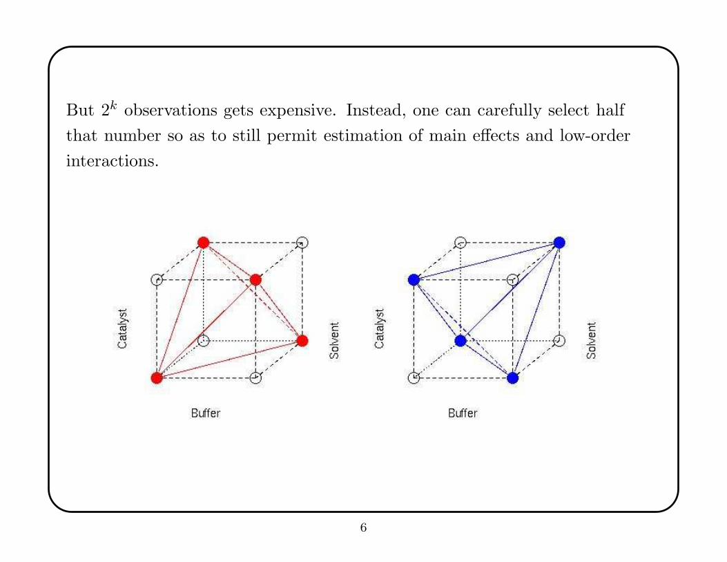
But 2k observations gets expensive. Instead, one can carefully select half

that number so as to still permit estimation of main effects and low-order

interactions.

6

Consider the 23−1 fractional factorial design (The previous figure gave two

illustrations.)

run A B C AB AC BC ABC obs

1 - - + + - - + Y112

2 + - - - - + + Y211

3 - + - - + - + Y121

4 + + + + + + + Y222

Note that because we have taken only half of the 8 observations needed for a

full factorial, some of the columns have identical entries.

Columns that have identical entries correspond to effects that are confounded

or aliased.

7

In order to estimate the effects, note that:

1

4(Y1 + Y2 + Y3 + Y4) = µ + (αβγ)

1

4(−Y1 + Y2 − Y3 + Y4) = α + (βγ)

1

4(−Y1 − Y2 + Y3 + Y4) = β + (αγ)

1

4(Y1 − Y2 − Y3 + Y4) = γ + (αβ)

Thus the estimate of the mean is confounded with the three-way interaction,

the estimate of the A effect is confounded with the BC interaction, the

estimate of the B effect is confounded with the AC interaction, and the

estimate of the C effect is confounded with the AB interaction.

If one assumes that there are no interactions, then one can make tests about

the main effects, or use a normal probability plot.

8

Note that we write 2k−p to denote a fractional factorial design in which each

factor has 2 levels, there are k factors, and we are taking a 1/2p fraction of the

number of possible factor level combinations.

In order to construct a fractional factorial that deliberately confounds

pre-selected factors, one needs to use a generator.

The generator uses the fact that squaring the entries in any given column gives

a column of ones, which can be thought of as an identity element I. If we

want to confound the A effect with the BC interaction, then that is equivalent

to declaring A ∗ BC = ABC = I. It follows that B = BI = B ∗ ABC = AC,

so B is confounded with the AC interaction. Similarly, C is confounded with

AB, and the overall mean (I) is confounded with ABC.

Here, the generator is the relationshiop I=ABC.

9

Consider a 24−1 fractional factorial design.

run A B C D AB AC BC ABC obs

1 - - - - + + + - Y1111

2 + - - + - - + + Y2112

3 - + - + - + - + Y1212

4 + + - - + - - - Y2211

5 - - + + + - - + Y1122

6 + - + - - + - - Y2121

7 - + + - - - + - Y1221

8 + + + + + + + + Y2222

10

What factors and interactions are confounded?

First, note that the ABC interaction has the same signs in its column as D.

Thus D and ABC are confounded, or D=ABC. This implies that I=ABCD is

the generator. (Why?)

¿From this, the confounding pattern is as follows:

A is confounded with BCD AB is confounded with CD

B is confounded with ACD AC is confounded with BD

C is confounded with ABD AD is confounded with BC

D is confounded with ABC ABCD is confounded with µ

11

One can go the other way, picking the generator and then deriving the

confounding pattern (and thus the design). For example, suppose we had

decided to confound D with AB.

In that case, the generator is I=ABD. Thus:

A is confounded with BD AC is confounded with BCD

B is confounded with AD ACD is confounded with BC

C is confounded with ABCD ABC is confounded with CD

D is confounded with AB ABD is confounded with µ

12

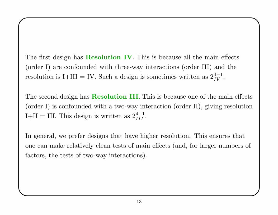
The first design has Resolution IV. This is because all the main effects

(order I) are confounded with three-way interactions (order III) and the

resolution is I+III = IV. Such a design is sometimes written as 24−1

IV .

The second design has Resolution III. This is because one of the main effects

(order I) is confounded with a two-way interaction (order II), giving resolution

I+II = III. This design is written as 24−1

III .

In general, we prefer designs that have higher resolution. This ensures that

one can make relatively clean tests of main effects (and, for larger numbers of

factors, the tests of two-way interactions).

13

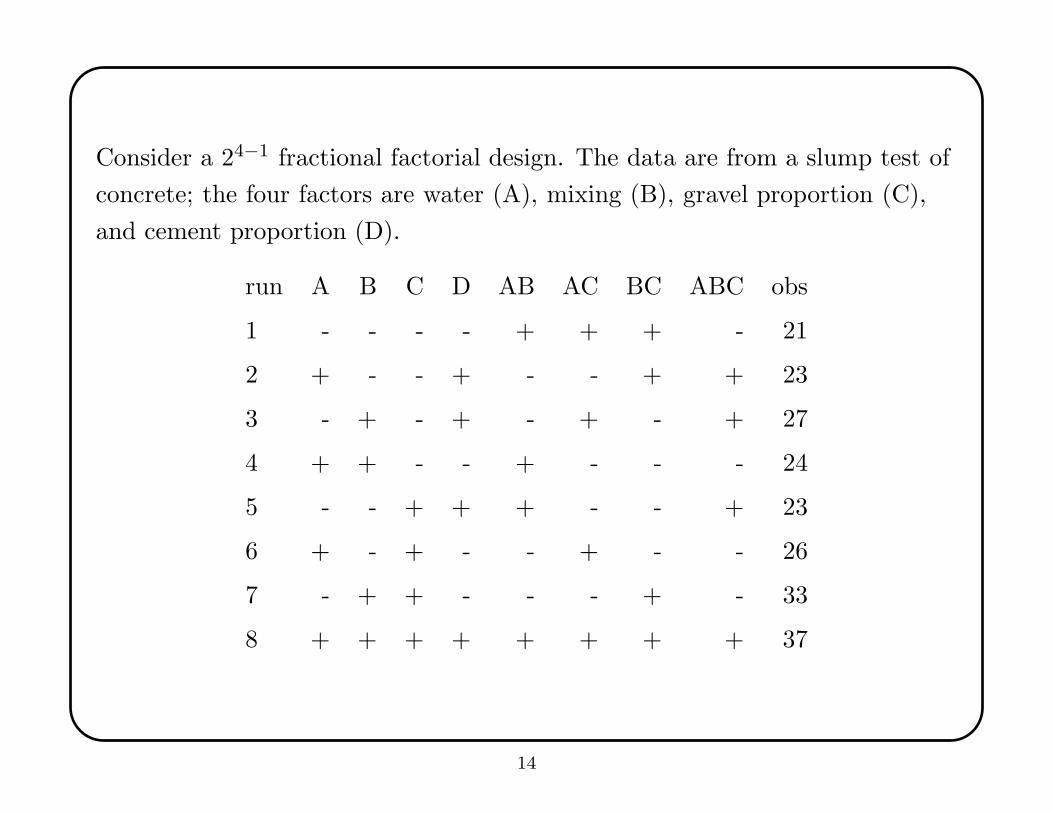
Consider a 24−1 fractional factorial design. The data are from a slump test of

concrete; the four factors are water (A), mixing (B), gravel proportion (C),

and cement proportion (D).

run A B C D AB AC BC ABC obs

1 - - - - + + + - 21

2 + - - + - - + + 23

3 - + - + - + - + 27

4 + + - - + - - - 24

5 - - + + + - - + 23

6 + - + - - + - - 26

7 - + + - - - + - 33

8 + + + + + + + + 37

14

26.75 = (y1 + · · · + y8)/8 = µ + ABCD

0.75 = (−y1 + y2 − y3 + y4 − y5 + y6 − y7 + y8)/8 = A + BCD

3.5 = B + ACD

3.0 = C + ABD

−.5 = (y1 − y2 − y3 + y4 + y5 − y6 − y7 + y8)/8 = AB + CD

1.0 = AC + BD

1.75 = BC + AD

.75 = (−y1 + y2 + y3 − y4 + y5 − y6 − y7 + y8) = D + ABC

If the null hypothesis of no effects is true, then the 3.5 and 3.0 look relatively

large. These deserve more study.

15

16.2 Higher-Order Fractions

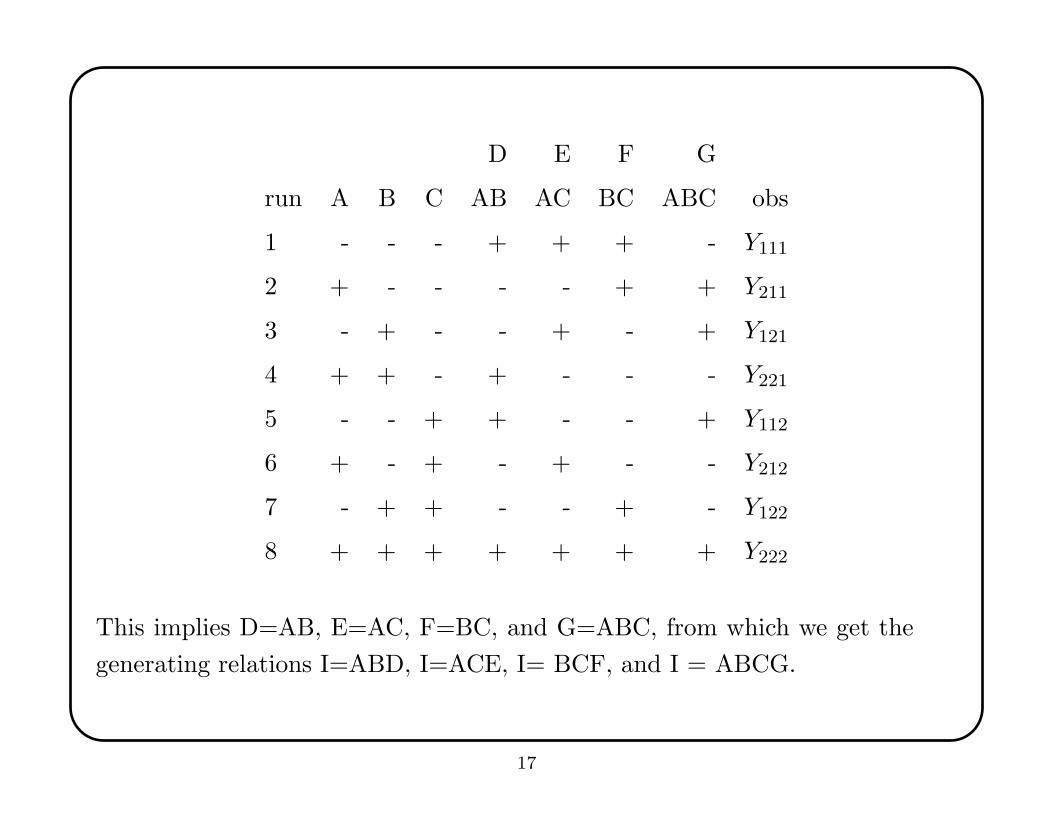
Consider an experiment designed to study seven factors in only eight runs.

This means we need a 27−4 fractional factorial design.

To do this, one needs more than one generator (in fact, one needs four

generators, since each halves the number of observations). One strategy is to

write out a full 23 factorial design, and then associate (confound or alias) the

interactions with each of the four additional factors.

16

D E F G

run A B C AB AC BC ABC obs

1 - - - + + + - Y111

2 + - - - - + + Y211

3 - + - - + - + Y121

4 + + - + - - - Y221

5 - - + + - - + Y112

6 + - + - + - - Y212

7 - + + - - + - Y122

8 + + + + + + + Y222

This implies D=AB, E=AC, F=BC, and G=ABC, from which we get the

generating relations I=ABD, I=ACE, I= BCF, and I = ABCG.

17

Since the product of I with itself is also I, then one can multiply any pair or

triple or quadruple of the generating relations and still get I. Thus:

I = ABD = ACE = BCF = ABCG

= BCDE = ACDF = CDG = ABEF

= BEG = AFG = DEF = ADEG

= BDFG = CEFG = ABCDEFG

This is cumbersome and tedious, but it enables one to calculate all the aliased

main effects and interactions.

This is called the defining relation.

18

If we multiply the defining relation by A, we find that

A = BD = CE = ABCF = BCG

= ABCDE = CDF = ACDG = BEF

= ABEG = FG = ADEF = DEG

= ABDFG = ACEFG = BCDEFG

Thus A is confounded with two-way, three-way, and higher interactions.

Similar calculations can be done for the other main effects. Each main effect is

confounded with a two-way interaction (e.g., G is confounded with CD, BE,

and AF. This means we have a 27−4

III design.

19

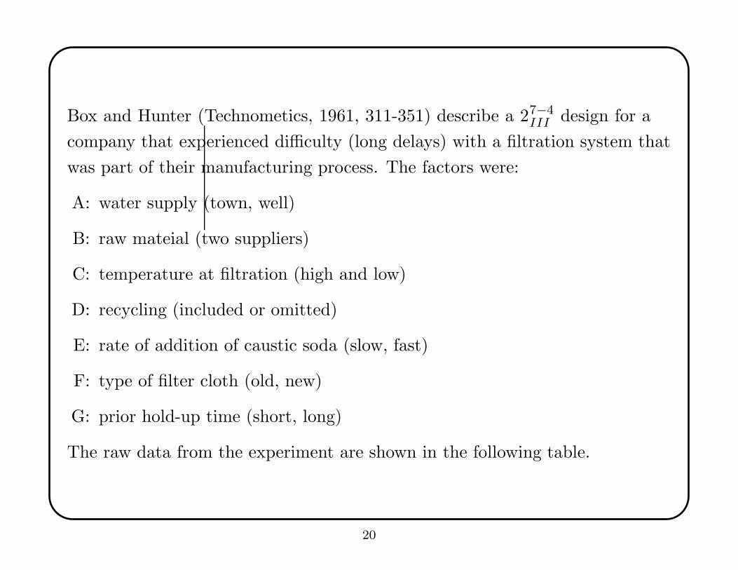
Box and Hunter (Technometics, 1961, 311-351) describe a 27−4

III design for a

company that experienced difficulty (long delays) with a filtration system that

was part of their manufacturing process. The factors were:

A: water supply (town, well)

B: raw mateial (two suppliers)

C: temperature at filtration (high and low)

D: recycling (included or omitted)

E: rate of addition of caustic soda (slow, fast)

F: type of filter cloth (old, new)

G: prior hold-up time (short, long)

The raw data from the experiment are shown in the following table.

20

D E F G

run A B C AB AC BC ABC obs

1 - - - + + + - 68.4

2 + - - - - + + 77.7

3 - + - - + - + 66.4

4 + + - + - - - 81.0

5 - - + + - - + 78.6

6 + - + - + - - 41.2

7 - + + - - + - 68.7

8 + + + + + + + 38.7

If one estimates the seven main effects (each of which is aliased with

interactions), one finds A is -5.4, B is -1.4, C is -8.3, D is 1.6, E is -11.4, F is

-1.7, and G is 0.3. It seems that E, C, and A (or corresponding interactions)

merit more thought.

21

These extreme fractions are difficult—one cannot get much information from,

say, eight observations, but these designs cleverly ensure that one gets the

most one can.

The designs are especially useful in stagewise experimentation. Often one

starts with a large set of factors, and then develops a series of fractional

factorial experiments that home in on the most important effects.

In the filtration experiment, the firm can now design follow-up experiments

that focus on the key factors. Or they can try to run their system at the high

levels of A, B, C, D, E, F, and G, which gave a filtration time of 38.7.

22

16.4 Exotic Designs

We have not talked about:

• Balanced Incomplete Block Designs

• Partially Balanced Incomplete Block Designs with k Associate Classes

• pk−r designs, or pj−rqk−s designs, and other generalizations

• Plackett-Burman designs, and other methods for response surface analysis

• D-optimality, G-optimality, E-optimality, and so forth.

• Repeated measures designs (MANOVA)

• ANACOVA

23