K = Shaft diameter, mm

Ka D < 300 (12 in.)\{Ka + K0) 300 < D < 600

\{Ka + K0 + Kp) D> 600 (or any D for slump > 70 mm)

In cemented sands you should try to ascertain the cohesion intercept and use a perimeter Xcohesion X L term. If this is not practical you might consider using about 0.8 to 0.9Kp.

The data base for this table includes tension tests on cast-in-place concrete piles rangingfrom 150 to 1066 mm (6 to 42 in.) in diameter. The rationale for these K values is that, with thesmaller-diameter piles, arching in the wet concrete does not develop much lateral pressureagainst the shaft soil, whereas the larger-diameter shafts (greater than 600 mm) allow fulllateral pressure from the wet concrete to develop so that a relatively high interface pressureis obtained.

16-15 LATERALLY LOADED PILES

Piles in groups are often subject to both axial and lateral loads. Designers into the mid-1960susually assumed piles could carry only axial loads; lateral loads were carried by batter piles,where the lateral load was a component of the axial load in those piles. Graphical methodswere used to find the individual pile loads in a group, and the resulting force polygon couldclose only if there were batter piles for the lateral loads.

Sign posts, power poles, and many marine pilings represented a large class of partiallyembedded piles subject to lateral loads that tended to be designed as "laterally loaded poles."Current practice (or at least in this textbook) considers the full range of slender vertical (orbattered) laterally loaded structural members, fully or partially embedded in the ground, aslaterally loaded piles.

A large number of load tests have fully validated that vertical piles can carry lateral loadsvia shear, bending, and lateral soil resistance rather than as axially loaded members. It is alsocommon to use superposition to compute pile stresses when both axial and lateral loads arepresent. Bowles (1974a) produced a computer program to analyze pile stresses when bothlateral and axial loads were present [including the P — A effect (see Fig. 16-21)] and forthe general case of a pile fully or partially embedded and battered. This analysis is beyondthe scope of this text, partly because it requires load-transfer curves of the type shown inFig. 16-18Z?, which are almost never available. Therefore, the conventional analysis for alaterally loaded pile, fully or partly embedded, with no axial load is the type considered inthe following paragraphs.

Early attempts to analyze a laterally loaded pile used the finite-difference method (FDM),as described by Howe (1955), Matlock and Reese (1960), and Bowles in the first edition ofthis text (1968).

Matlock and Reese (ca. 1956) used the FDM to obtain a series of nondimensional curvesso that a user could enter the appropriate curve with the given lateral load and estimate theground-line deflection and maximum bending moment in the pile shaft. Later Matlock andReese (1960) extended the earlier curves to include selected variations of soil modulus withdepth.

Previous Page

Although the nondimensional curves of Matlock and Reese were widely used, the au-thor has never recommended their use. A pile foundation is costly, and computers have beenavailable—together with computer programs—for this type of analysis since at least 1960.That is, better tools are now available for these analyses.

THE p-y METHOD. The initial work on the FDM lateral pile solution [see McClelland andFocht (1958)] involved using node springs p and lateral node displacements y, so that usersof this method began calling it the "p-y method." Work continued on this FDM computerprogram to allow use of different soil node springs along the pile shaft—each node having itsown p-y curve [see Reese (1977)]. Since p-y curves were stated by their author to representa line loading q (in units of kip/ft, which is also the unit of a soil spring), user confusion anduncertainty of what they represent has developed. This uncertainty has not been helped bythe practice of actually using the p part of the p-y curve as a node spring but with a 1-ft nodespacing so that it is difficult to identify exactly how/? is to be interpreted. The product of nodespring and node displacement y gives p • y = a node force similar to spring forces computedin the more recognizable form of force = K • X.

The data to produce a/?-y curve are usually obtained from empirical equations developedfrom lateral load tests in the southwestern United States along the Gulf Coast. In theory, oneobtains a p-y curve for each node along the pile shaft. In practice, where a lateral load testis back-computed to obtain these curves, a single curve is about all that one can develop thathas any real validity since the only known deflections are at or above the ground line unlessa hollow-pipe pile is used with telltale devices installed. If the node deflection is not known,a p-y curve can be developed with a computer, but it will only be an approximation.

The FDM is not easy to program since the end and interior difference equations are notthe same; however, by using 1-ft elements, interior equations can be used for the ends withlittle error. The equations for the pile head will also depend on whether it is free or eithertranslation and/or rotation is restrained. Other difficulties are encountered if the pile sectionis not constant, and soil stratification or other considerations suggest use of variable lengthsegments. Of course, one can account for all these factors. When using 1-ft segments, justshift the critical point: The maximum shift (or error) would only be 0.5 ft.

The FDM matrix is of size NxN, where TV = number of nodes. This matrix size anda large node spacing were advantages on early computers (of the late 1950s) with limitedmemory; however, it was quickly found that closer node spacings (and increases in AO pro-duced better pile design data. For example, it is often useful to have a close node spacing inabout the upper one-third of a pile.

The FDM would require all nodes to have equal spacing. For a 0.3-m spacing on a 36-mpile, 121 nodes would be required for a matrix of size NXN = 14 641 words or 58.6 kbytes(4 bytes/word in single precision). This size would probably require double precision, so thematrix would then use 117 kbytes.

THE FEM LATERAL PILE/PIER ANALYSIS. The author initially used the FDM for lateralpiles (see first edition of this text for a program); however, it soon became apparent thatthe FEM offered a significant improvement. Using the beam element requires 2 degrees offreedom per node, but the matrix is always symmetrical and can be banded into an array ofsize

2 X number of nodes X Bandwidth

This array is always 2 X NNODES X 4, thus, a pile with 100 nodes would have a stiffnessmatrix of 2 X 100 X 4 = 800 words. This is 3200 bytes or 3.2k of memory and in doubleprecision only requires 6.4k bytes.

One advantage of the FEM over the FDM is the FEM has both node translation and ro-tation, whereas the FDM only has translation. The elastic curve is somewhat better definedusing both translation and rotation.

Another advantage is that the element lengths, widths, and moments of inertia can varywith only slightly extra input effort. One can even use composite piles. The pile modulusof elasticity is usually input as a constant since most piles are of a single material, but it istrivial to modify the moment of inertia for a composite section so that the program computesthe El/L value correctly. This value is determined by computing a modified moment of inertiaIm as in Eq. (13-4).

When using variable element lengths it is suggested that one should try to keep the ratioof adjacent element lengths (longest/shortest) < 3 or 4.

A major advantage of the FEM is the way in which one can specify boundary cases (nodeswith either zero rotation or translation) and lateral loads. The FDM usually requires the loadand boundary points be pre-identified; the FEM allows any node to be used as a load point orto have known translation or rotation—the known value is usually 0.0 but can be nonzero aswell.

A final advantage is that the FEM for a lateral pile program can be used for a lateral pier(piles with a larger cross section) or beam-on-elastic-foundation design. It is only necessaryto input several additional control parameters so the program knows what type of problem isto be solved. Thus, one only has to learn to use one fairly simple program in order to solve sev-eral classes of problems. Your sheet-pile program FADSPABW (B-9) is a special case of thismethod. It was separately written, although several subroutines are the same, because thereare special features involved in sheet-pile design. These additional considerations would in-troduce unnecessary complexity into a program for lateral piles so that it would be a littlemore difficult to use. Many consider it difficult in any case to use a program written by some-one else, so the author's philosophy has been to limit what a program does so that it is easierto use.

Refer to Sec. 9-8 for the derivation of the stiffness matrix and other matrices for the beam-on-elastic foundation and also used for the lateral pile. The only difference is that the beam-on-elastic foundation is rotated 90° clockwise for the lateral pile P-X coding and the endsprings are not doubled (see Fig. 16-19). You must know how the finite-element model iscoded and how the element force orientations (direction of arrowheads on force, moment,and rotation vectors) are specified either to order the input loads or to interpret the outputelement moments and node displacements.

USING THE FEM COMPUTER PROGRAM. The general approach to setting up an FEMmodel for using your diskette program FADBEMLP (B-5) to analyze lateral piles is this:

1. Divide the pile into a convenient number of elements (or segments) as in Fig. 16-19. Fromexperience it has been found that the top third of the embedment depth is usually criticalfor moments and displacements, so use shorter element lengths in this region. Avoid veryshort elements adjacent to long elements; place nodes at pile cross-sectional changes, atsoil strata changes, and where forces or boundary conditions are being applied. Generally10 to 15 elements are adequate, with 4 to 8 in the upper third of the embedded shaft length.

Figure 16-19 Laterally loaded pile using finite elements. Typical loadings shown in (a) and (b). Note that elementsdo not have to be same size or length. Generally use short elements near ground surface and longer elements nearpile point where moments are less critical.

2. Partially embedded piles are readily analyzed by using JTSOIL equal to the node wheresoil starts (same as for sheet-pile wall). Use JTSOIL = 1 if ground line is at first pile node.

3. Identify any nodes with zero translation and/or rotation. NZX = number of Xs of zero dis-placement. Use element coding to identify those X values that are input using NXZERO(I).

4. Make some estimate of the modulus of subgrade reaction and its depth variation (AS, BS,EXPO). Note that either AS or BS can be zero; EXPO = 0.5, 0.75, 1.0, or 1.5 may beappropriate; EXPO is the exponent of Zn. You can also estimate a Z^-value [and XMAX(I)]for each node to input similar to the sheet-pile program.

5. Back-compute lateral load test data, if they are available, for the best estimate of ks. Oneshould not try to back-compute an exact fit since site variability and changes in pile type(pipe versus HP) preclude the existence of a unique value of ks. The large number of piletests reported by Alizadeh and Davisson (1970) clearly shows that great refinement inback computations is not required. One should, however, use in a load test the lateral loadthat is closest to the working load for best results.

WHAT TO USE FOR THE MODULUS OF SUBGRADE REACTION ks.5 The modulus of

subgrade reaction is seldom measured in a lateral loaded pile test. Instead, loads and deflec-

5It should be understood that even though the term ks is used in the same way as for the beam-on-elastic foundation,it is a vertical value here. The type (vertical or horizontal) is identified to the user by the context of usage.

Rotation—no translation Translation—no rotation

JTSOIL - 1

JTSOIL a 4

element -numbers

Node

NM = 6NNODES =NM+1=6+1=7NP = 14 = 2 x NNODES NM = 8

NNODES = NM + 1 = 9

N P = 18

(a) Fully embedded (b) Partially embedded.

(c) General ith elementP-X coding andelement forces.

tions are usually obtained as well as, sometimes, bending moments in the top 1 to 3 m ofthe embedded pile. From these one might work back using one's favorite equation for lateralmodulus (or whatever) and obtain values to substantiate the design for that site.

Node values (or an equation for node values) of ks are required in the FEM solution forlateral piles. Equation (9-10), given in Chap. 9 and used in Chap. 13, can also be used here.For convenience the equation is repeated here:

^ = A , + BsZn (9-10)

If there is concern that the ks profile does not increase without bound use Bs = 0 or useBs in one of the following forms:

Bs ( | j = ^ Z " = B'sZn (now input B's for B5)

or use B5(Z)" where n < 1 (but not < 0)

where Z = current depth from ground surface to any node

D = total pile length below ground

The form of Eq. (9-10) for ks just presented is preprogrammed into program FADBEMLP(B-5) on your diskette together with the means to reduce the ground line node and next lowernode ks (FACl, FAC2 as for your sheet-pile program). You can also input values for theindividual nodes since the soil is often stratified and the only means of estimating ks is fromSPT or CPT data. In this latter case you would adjust the ground line ks before input, theninput FACl = FAC2 = 1.0.

The program then computes node springs based on the area Ac contributing to the node,as in the following example:

Example 16-9. Compute the first four node springs for the pile shown in Fig. El 6-9. The soilmodulus is ks = 100 + 50Z05. From the ks profile and using the average end area formula:

Summary,

,etc.

Example 16-9 illustrates a basic difference between this and the sheet-pile program. Thesheet-pile section is of constant width whereas a pile can (and the pier or beam-on-elasticfoundation often does) have elements of different width.

This program does not allow as many forms of Eq. (9-10) as in FADSPABW; however,clever adjustment of the BS term and being able to input node values are deemed sufficientfor any cases that are likely to be encountered.

In addition to the program computing soil springs, you can input ks = 0 so all the springsare computed as Ki = 0 and then input a select few to model structures other than lateral piles.Offshore drilling platforms and the like are often mounted on long piles embedded in the soilbelow the water surface. The drilling platform attaches to the pile top and often at severalother points down the pile and above the water line. These attachments may be modeled assprings of the AE/L type. Treating these as springs gives a partially embedded pile model—with possibly a fixed top and with intermediate nonsoil springs and/or node loads—with thebase laterally supported by an elastic foundation (the soil).

Since the pile flexural stiffness EI is several orders of magnitude larger than that of thesoil, the specific value(s) of ks are not nearly so important as their being in the range of 50 toabout 200 percent of correct. You find this comparison by making trial executions using a Ic5,then doubling it and halving it, and observing that the output moments (and shears) do notvary much. The most troublesome piece of data you discover is that the ground line displace-ment is heavily dependent on what is used for ks. What is necessary is to use a pile stiff enough

Figure E16-9

Projected pile width, m

ks = Profile

and keep the lateral load small enough that any computed (or actual) lateral displacement istolerable.

A number of persons do not like to use the modulus of subgrade reaction for anything—beams, mats or lateral piles. Generally they have some mathematical model that purportedlyworks for them and that they would like for others to adopt. In spite of this the ks concepthas remained popular—partly because of its simplicity; partly because (if properly used) itgives answers at least as good as some of the more esoteric methods; and, most importantly,because A is about as easy to estimate as it is to estimate the stress-strain modulus Es andPoisson's ratio /JL.

WHAT PILE SECTION TO USE. It is usual to use the moment of inertia / of the actual pilesection for both HP and other piles such as timber and concrete. For reinforced concrete piles,there is the possibility of the section cracking. The moment of inertia / of a cracked sectionis less than that of the uncracked section, so the first step in cracked section analysis is torecompute / based on a solid transformed section, as this may be adequate.

It is suggested that it is seldom necessary to allow for section cracking. First, one shouldnot design a pile for a lateral load so large that the tension stresses from the moment producecracking—instead, increase the pile cross section or the number of piles. Alternatively, usesteel or prestressed concrete piles.

The possibility of concrete pile cracking under lateral load is most likely to occur when par-tially embedded piles are used. The unsupported length above the ground line may undergolateral displacements sufficiently large that the section cracks from the resulting mtfment-induced tension stresses. The unsupported pile length must be treated similarly to an unsup-ported column for the structural design, so a larger cross section may be required—at least inthe upper portion of the pile.

16-15.1 Empirical Equations for Estimating ks

Where pile-load tests are not available, some value of ks that is not totally unrealistic mustbe estimated, one hopes in the range between ± 50 and ± 200 percent6 of the correct value.The following equations can be used to make reasonable estimates for the lateral modulus ofsubgrade reaction.

An approximation proposed by the author is to double Eq. (9-9) since the soil surroundsthe pile, producing a considerable side shear resistance. For input you obtain ASf Bs valuesand multiply by two. Using the bearing-capacity components of Eq. (13-1) to give the neededparts of Eq. (9-9), we have

As = AS = C(cNc + 0.5yBpNy)

BsZn = BS*(Z~N) = C(yNqZ

])

where C = 40 for SI, 12 for Fps. It was also suggested that the following values could beused, depending on the actual lateral displacement:

6Two hundred percent is double the true value, and 50 percent is one-half the true value.

For AH, C

SI(m) Fps(in.) SI Fps IC

0.0254 1 40 (12) 800.006 \ 170 (48) 3400.012 \ 80 (24) 1600.020 \ 50 (36) 100

16-15.2 Size and Shape Factors

The idea of doubling the lateral modulus was to account for side shear developed as thepile shaft moves laterally under load, both bearing against the soil in front and shearing thesoil on parts of the sides as qualitatively illustrated in Fig. 16-20. Clearly, for piles with asmall projected D or B, the side shear would probably be close to the face bearing (consistingof 1.0 for face +2 X 0.5 for two sides = 2.0). This statement would not be true for largerD or B values. The side shear has some limiting value after which the front provides theload resistance. Without substantiating data, let us assume this ratio, two side shears to oneface, of 1:1 reaches its limit at B = D = 0.457 m (18 in.). If this is the case then the sizefactor multiplier (or ratio) Cm should for single piles be about as follows (the 1.0 is the facecontribution):

For Ratio, Cm

Lateral loads of both Px and Py

(face 4- 1 side) 1.0 + 0.5B = D < 0.457 m 1.0 + 2 X 0.5

( . _ - \0.75> 1.5

D, mm Juse 1.0 + 0.25 for D > 1200mm

You should keep the foregoing contributing factors in mind, for they will be used later wherethe face and side contributions may not be 1.0 and 0.5, respectively.

Now with Cw, rewrite Eq. (13-1) as used in Sec. 16-15.1 to read

As = AS = CmC(cNc + 0.5yBpNy)}

BsZn = BS * Z~N = CmC(yNqZ

n) J

It is also suggested that the BS term should use an exponent n that is on the order of 0.4to 0.6 so that ks does not increase without bound with depth.

Research by the author by back-computing ks from piles in cohesionless soils at the samesite indicates that Eq. (9-10) should be further rewritten to read

A8 = AS = FwlCmC(cNc + 0.5y BpN7)] (\6-26a)BsZ

n = BS * Z^N = Fw2CmC(yNqZn) J

where Fw\, Fw2 = 1-0 for square and HP piles (reference modulus)Fw\ = 1.3 to 1.7; FW2 = 2.0 to 4.4 for round piles

One probably should apply the Ft factors only to the face term (not side shear) for roundpiles. Whether these shape factors actually result from a different soil response for roundpiles or are due to erroneous reported data from neglecting the distortion of the hollow pipe(laterally into an oblate shape) under lateral load is not known at this time. Gleser (1983) andothers have observed that the response of a round pile is different from that of a square orHP pile, in general agreement with the foregoing except in a case where a comparison of a100-mm HP pile to a 180-mm diameter pipe pile was claimed not to produce any noticeabledifference.

side bearing

(b) Circular pileFigure 16-20 Qualitative front and side resistancesfor a lateral pile.

side bearing

(a) Square of rectangular

side shear

face

bea

ring

side shear

back

pile

fron

t

pile

Size and projection widths would make it very difficult to note any differences in thiscase, particularly if the pipe wall thickness was such that the diameter did not tend to oblate(flatten).

USING THE GIVEN BEARING CAPACITY. If we have only the allowable bearing pressureqa, we can use Eq. (16-26) as follows (but may neglect the Nq term):

ks = FH,,i X SF X CmC Xqa + Fw>2 X CmCyZnNq (16-26/?)

where SF = safety factor used to obtain qa (usually 3 for clay; 2 for cohesionless soil)Nq = value from Table 4-4 or from Eq. (16-7) or (16-7J)

n = exponent as previously defined; 1 is probably too large so use about 0.4 to 0.6so ks does not increase too much with depth

If you use either Eq. (16-26) or (16-26a) you should plot ks for the pile depth using severalvalues of exponent n to make a best selection.

It has been found that the use of Eq. (16-26) produces values within the middle to upperrange of values obtained by other methods.

If we take qa = qu (unconfined compression test) and omit the Nq term in Eq. (\6-26a),the value of ks in Fps units for a pile of unknown B is

ks = Cm X 12 X SF X qu = 2 X 3 X 12 X qu = 12qu

Davisson and Robinson (1965) suggested a value of ks ~ 67 su, which was about half of 12qu.Later Robinson (1978) found that 61 su was about half the value of ks indicated by a series oflateral load tests [that is, 12qu (or 24Oq u, kPa) was about the correct value].

The API (1984) suggests that the lateral bearing capacity for soft clay (c < 50 kPa) belimited to 9c and for stiff clay from 8c to 12c [see Gazioglu and O'Neill (1985) for detaileddiscussion]. In soft clay this bearing capacity would give, according to Eq. (16-26a), the value

ks = Cm(40)(9c) = 360Cmc (kN/m3)

which does not appear unreasonable.You may indirectly obtain ks from the following type of in situ tests:

a. Borehole pressuremeter tests where Epm = pressuremeter modulus

*, = ^ 1 (16-27)Bp

For cohesionless soils [see Chen (1978)]:

(16-27a)

(16-276)

And for cohesive soils:

where Ed = dilatometer modulus, kPa or ksf

Fp = pile shape factor: 1.5 to 4.0 for round piles; 1.0 for HP or square piles

For these values of ks you would compute values as close to your pile nodes as possibleand input the several node values, not just a single value for the full depth.

The stress-strain modulus Es can be used in Eq. (16-31) following [or Vesic's Eq. (9-6),given earlier] to compute ks. Estimate Es from your equation or method or one of the follow-ing:

a. Triaxial tests and using the secant modulus Es between 0 and 0.25 to 0.5 of the peakdeviator stress. The initial tangent modulus may also be used. Do not use a plane strainEs.

b. The standard penetration test [see Yoshida and Yoshinaka (1972)] to obtain

Es = 650N kPa (16-29)

This equation has a maximum error of about 100 percent with an average error of closeto ± 20 percent. Assume that N in Eq. (16-29) is NJO (see under donut hammer of Table3-3).

For CPT data convert to equivalent SPT TV and use Eq. (16-29).c. Use consolidation test data to obtain mv to compute the stress-strain modulus by combining

Eqs. (2-43) and Eq. (J) of Sec. 2-14 and noting

A// _ 1

to obtain

Es = 3 { 1 - 2 ^ (16-30)mv

Any of these three values of Es can be used to compute ks in clay using any of the followingthree equations cited by Pyke and Beikae (1983):

0.48 to 0.90^,ks = - (a)

where 0.48 is for HP piles; 0.9 for round piles (i.e., a shape factor Fw\ ~ 2);

K - ^ W

and for sands

(C)

b. Flat dilatometer tests:

(16-28)

where in Eq. (c) Es = triaxial test value at about 6—0.01. You may also use these stress-strain moduli values in the following equation [Glick (1948)] to obtain a modified A that isthen used in Eq. (16-32):

" • ( u ^ - W M V U - u m i <u"itsofE') <1M1)

where Lp = pile length, m or ftB = pile width, m or ft

After computing k's, convert it to the usual ks using the following:

ks = % (16-32)D

Since this value of k's has the same meaning as the Vesic value given by Eq. (9-6), we canuse that equation with the following suggested modification:

k 7n

ks = - ^ - (l6-32a)

The zn term is suggested to allow some controlled increase in ks with depth.The NAFAC Design Manual DM7.2 (1982) suggests the following:

k5 = ^ (16-33)

where / = factor from following table, kN/m3 or k/ft3

D = pile diameter or width, m or ftz = depth; m or ft gives ks = O at ground surface and a large value for long piles at

the tips. A better result might be had using (z/D)n where n ranges from about0.4 to 0.7.

Values for/ (use linear interpolation)

Fine-grained:

Coarse-grained:

20406080

110150190230270310370

Dr

0

15

30405060708090

/

200350550800

800140020002800340042004900

TABLE 16-4

Representative range of values of lateralmodulus of subgrade reaction (value of As

in the equation ks = As + Bzn

Soil* ks, kef ks, MN/m3

Dense sandy gravel 1400-2500 220-400Medium dense coarse sand 1000-2000 157-300Medium sand 700-1800 110-280Fine or silty, fine sand 500-1200 80-200Stiff clay (wet) 350-1400 60-220Stiff clay (saturated) 175-700 30-110Medium clay (wet) 250-900 39-140Medium clay (saturated) 75-500 10-80Soft clay 10-250 2 ^ 0

"'Either wet or dry unless otherwise indicated.

Table 16-4 gives ranges of ks for several soils, which are intended as a guide for probablevalues using more precise methods—or at least using the site soil for guidance. They shouldbe taken as reasonably representative of the As + Bs terms at a depth from about 3 to 6 m andfor pile diameters or widths under 500 mm.

16-15.3 Nonlinear Effects

It is well known that doubling the load on a lateral pile usually more than doubles the lateraldisplacement and increases the bending moment. The moment increase results from both theincrease in Sh and the greater depth in which lateral displacements occur. Both of these effectsresult from nonlinear soil behavior idealized by the curve shown in Fig. 2-43c, particularly athigher stress levels a that result from larger lateral loads. Usually the lateral displacementsin the load range of interest are in that part of the a-8 curve that is approximately linear.

In the curve of Fig. 2-43c the modulus of subgrade reaction is taken as a "secant" linefrom the origin through some convenient stress value a. Ideally one should have a curvesuch as this for each node point (see Fig. E13-le) for a lateral pile. Then, as a displacementis computed one would enter the curve, obtain a revised secant modulus ks, and recomputethe displacements until the 5^ value used = S value obtained.

This approach is seldom practical since these curves are difficult to obtain—usually a pipepile must be used for the test so that lateral measurements can be taken at nodes below theground line. A pipe pile, however, has a shape factor, so the results are not directly usable forother pile shapes.

Most lateral piles are designed on the basis of using penetration testing of some kind,supplemented with unconfined compression data if the soil is cohesive. For these cases thetwo-branch nonlinear model proposed by the author (see Fig. 9-9c) will generally be ade-quate.

The program FADBEMLP on your diskette allows you to model the two-branch nonlinearnode displacement curve for the soil as you did in program FADSPABW. That is, you caninput the maximum linear displacement at each node as XMAX(I) and activate a nonlin-ear check using the control parameter NONLIN > 0. Here a negative displacement is not asoil separation, but rather the pile has deflected forward such that the elastic line has produced

a displacement at a lower node against the soil behind the pile. An extensive discussionof XMAX(I) was given in Chap. 13 that will not be repeated here except to note that thenonlinear check is |X(I)| < XMAX(I).

CYCLIC LOADING. The ks for cyclic loading should be reduced from 10 to 50 percent ofthat for static loading. The amount of reduction depends heavily on the displacements duringthe first and subsequent cycles.

Quasi-dynamic analysis of offshore piles subject to wave forces can be obtained by apply-ing the instant wave force on the nodes in the water zone for several closely spaced discretetime intervals.

DISPLACEMENTS FROM SOIL CREEP. Lateral displacement from long-term loading, pro-ducing secondary consolidation or creep, has not been much addressed for lateral piles. Kup-pusamy and Buslov (1987) gave some suggestions; however, the parameters needed for thenecessary equations are difficult to obtain. Although one could consult that reference, theirequations are little better than simply suggesting that, if the lateral load is kept under 50 per-cent of the ultimate, the creep displacement for sand after several years is not likely to exceed10 percent of the initial lateral displacement.

For clay, the creep will depend on whether it is organic or inorganic. The creep displace-ment may be as much as the initial displacement for an organic clay but only about 15 to 20percent for an inorganic one. One might compute a lateral influence depth of approximately5 X projected width of pile/pier = Hf and use Eq. (2-49) for a numerical estimate if youhave a secondary compression coefficient Ca.

Laterally loaded piles in permafrost also undergo creep. Here the creep depends on the tem-perature, quantity and type of ice, and the lateral pressure, generally expressed as a "creep"parameter. Neukirchner (1987) claims to have a reasonable solution, but the creep parameteris so elusive that there is substantial uncertainty in any permafrost creep estimate.

When lateral piles undergo creep, the effect is to increase the lateral displacement andbending moment. The goal is an estimate of the final lateral displacement and bending mo-ment. The bending moment might be obtained in any situation where creep is involved bysimply measuring the displacements and, using the current lateral displacement as the spec-ified displacement in program FADBEMLP, computing the moment produced by that dis-placement.

Alternatively since creep decreases approximately logarithmically it might be obtainedby plotting the displacement at several time intervals (long enough to be meaningful) andnumerically integrating the curve to find the anticipated total lateral displacement for inputso as to compute the lateral pile bending moments.

16-15.4 Including the P-A Effect

The P-A effect can be included for lateral piles (refer to Fig. 16-21) in a straightforwardmanner as follows:

1. Draw the partially embedded pile to rough scale, code the nodes, and locate the nodeJTSOIL. We will use JTSOIL as the reference node.

2. Make an execution of the data with the horizontal force Ph located at the correct nodeabove JTSOIL. This will generally be at the top of the pile where the vertical load Pv also

P - A moment at node JTSOILJTSOIL

•Nodes

JTSOIL

Figure 16-21 The geometric P-A effect for laterally loaded piles.

acts. Until you become familiar with program FADBEMLP you should use the pile andload geometry which corresponds to Fig. 16-21.

3. Inspect the output, and at the top node where Pv acts there will be a lateral displacement(let us use, say, A = 0.40 m and a vertical force Pv = 60 kN). From the lateral displace-ment, which is with respect to the original position of node JTSOIL, a P - A moment canbe computed (see inset of Fig. 16-21) of 60 X 0.40 = 24 kN-m.

4. Make a copy of the original data and change NNZP from 1 (for the horizontal force only)to 2 to include both the original horizontal force and the P - A moment just computed of 24kN- m. If we assume JTSOIL = 11, the moment NP location is 2 X 11 - 1 = 21 .

5. In the data file you can see the horizontal load and its NP number. Just below, enter 21 andthe moment value of 24. Note from the inset, however, that the moment has a negativesign. The two load matrix entries would now read

Node Load2 Pf1 (this is the problem value)

21 - 2 4 . 0

Given: 0 = 32°; /5 = 0°; 8 = 20°

unfactored ks = 200 + 4OZ"; Coulomb / ^ = 6.89 (a = 90°)

a = 100° -> A^ = 11.35 (use prog. FFACTOR) a = 80°-> K^ = 4.89

Cm = 11.35/6.89 + 2(0.5) = 2.65 C1n = 4.89/6.89 + 2(0.5) =1.71

^ = 2.65(200 + 400Zn) ks= 1.71(200 + 400Z")

= 530 + 1060Z" = 342 + 684Z"

(a) Definition of batter angle a for adjustment of C1n for ks.

Figure 16-22 Adjusting ks factor Cm for pile batter and spacing and/or location in group.

6. Now execute this data set (if the sign is correct the top node displacement A will slightlyincrease). Obtain the displacements, and if the previous Ap - Acurrent — some convergence(not in program but decided by the user), say, 0.005 m or less, stop. Otherwise continueto compute a new P-A moment and recycle.

Note that the second data set has two changes initially: (1) to increase NNZP by 1 and (2)to input the P-A moment. After this, the only change to that second data set is to reinput thenew P-A moment until the problem converges.

The node JTSOIL will probably move laterally also, and the most critical P-A moment isnot the difference between the top node and node JTSOIL but between the top node and somenode farther down that does not move laterally. You could, of course, put the P-A momentat this location, but the foregoing suggested solution is generally adequate. You can also usethe difference between the top translation and the computed translation at node JTSOIL, butthis is less conservative.

16-15.5 Lateral Piles on Slopes

Laterally loaded piles are frequently sited on slopes, for example, power poles and bridgefoundations. It is suggested that the same procedure be used to reduce the lateral ks val-ues as was used for the sheet-pile wall case. That is, use program WEDGE or FFACTOR to

Rear Rear

Front Front

(b) Pile spacing s' and location for cm adjustments for ks.

compute the passive force (or coefficient Kp) case for the horizontal ground line and for theactual ground slope and use the ratio RF as in Eq. (13-3). Because the side shear part fromfactor Cm is not required to be reduced, you should apply the slope ratio RF only to the face(or bearing) part of &s. For example, compute ks = 2000 based on using Cm = 2; RF = 0.6.This calculation gives ks\ = 2000/Cm = 1000 = ks2. The revised ks = ks2 + RF X ^ 1 =1000 + 0.6 x 1000 = 1600.

16-15.6 Battered Piles

The ks for battered piles has not been addressed much in the literature. In the absence ofsubstantiating data the author suggests (see Fig. 16-22^) the following:

1. Compute the Coulomb passive earth pressure coefficient Kp for a vertical wall (a = 90°),including any slope angle /3. A lateral pile is a "passive" earth-pressure case but requiresincluding side shear effects since the Coulomb case is one of plane strain.

2. Next draw the battered pile and place a perpendicular load on the pile with the (+) di-rection as shown on Fig. 16-22a. The perpendicular load direction should correspond tothat used to establish the batter direction [will be either (+) or (-)]. Draw a horizontalcomponent line as, say, Px as shown.

3. Now measure (or compute) the batter angle a. It is counterclockwise from a horizontalline at the pile tip for the (+) load perpendicular; it is clockwise for a (-) load perpendic-ular. For the (+) perpendicular shown on Fig. \6-22a we have a > 90° if the horizontalcomponent is below and a < 90° if the horizontal component is above the perpendicular.

4. Compute a Coulomb passive pressure coefficient Kpb for the applicable batter angle a.Use program FFACTOR. You probably should include a pile-to-soil friction angle 8.

Side

Corner

5. Compute a revised ks as

ks = 11.0 x ^ U (2 x 0.5)

This calculation should give the expected result of a larger ks for a > 90° and a smaller&5 for a < 90° for the (+) case shown on Fig. 16-22a.

Note: We only adjust the face or bearing part of ks because the side shear should be aboutthe same for either a vertical or a battered pile.

16-15.7 Adjusting ks for Spacing

It is generally accepted that there is a reduction in the lateral subgrade modulus ks when pilesare closely spaced. Poulos (1979) suggested using factors from curves developed using anelastic analysis of pile-soil interaction (i.e., Es, /x,), which are then combined to give a groupfactor. This method does not seem to be used much at present.

The following method (refer to Fig. 16-22&) is suggested as an easy-to-visualize alternativeto obtain the lateral modulus for individual piles in a group:

1. Referring to the Boussinesq pressure bulb (Fig. 5-4) beneath a rectangular footing, wesee that at a D/B > 6 the pressure increase on the soil is negligible. So, using a clearpile spacing s' for depth D and pile projected width for B, we can say that if s'/B > 6 noadjustment in ks is necessary.

2. For spacings of s'/B < 6 use Fig. 5-4 ("Continuous") and multiply the face bearing termby (1.0 - interpolated pressure intensity factor). For example at s'/B = 2, we obtain 0.29,and the face term is 1.0 X (1.0 - 0.29) = 0.71 (here 0.29, or 29 percent, of the pressureis carried by the front pile). This is the face factor contribution to Cm (= 2 sides + face= (2 X 0.5)+ 0.71 = 1.71).

3. For the side shear factor contribution to Cm we have two considerations:a. Location (corner, front, side, interior, or rear)b. What reduction factor (if any) to use

Clearly for side and corner piles one side is not affected by any adjacent pile so for thosewe have some interior side interaction factor ^ + an exterior factor of 0.5. For front, interior,and rear piles we have a side interaction factor of 2W.

One option is to consider that any pile insertion increases the lateral pressure so that theuse of ^ = 0.5 is adequate. Another option is to consider that enough remolding takes placethat the soil is in a residual stress state and to reduce the 0.5 side factor to

, _ Residual strengthUndisturbed strength

16-15.8 Estimating Required Lengthof a Laterally Loaded Pile

The required length of a laterally loaded pile has not been directly addressed in the literature.Obviously, it should be long enough to provide lateral stability, and if there is an axial load,the pile must be long enough to develop the required axial capacity.

We can obtain the required pile embedment length for lateral stability (it was previouslynoted that usually the upper one-third of the pile actively resists the lateral loads) as follows:

1. Compute the embedment length required for any axial load. If there is no axial load ini-tially, try some reasonable length, say, L'.

2. Use computer program B-5 with your lateral load Py1 and obtain a set of output.

3. Inspect the horizontal displacement 8hp at the pile base (or point). If the absolute valueof Shp ~ 0.0, the pile length is adequate. If \Shp\ > 0.0, you have to decide whether thelength is adequate, since this amount of displacement may be indicative of a toe kickout(lateral soil failure). Also check that the active (zone of significant bending moment) depthis approximately L'/3. Now do two other checks:a. Depending on how you initialized L\ you may want to increase it by 20 to 30 percent

to allow for a modest stability number (SF).b. Make two additional program executions using 1/2 and 2 times the initial value of

lateral subgrade modulus ks. If both these executions give 8hP ~ 0.0, you have anadequate pile embedment depth L'. If 8hp > 0.0 (particularly for the ks/2 case), youprobably should increase L'.

If you increase L' based on either (a) or (ft), you should recycle to step 2. When you findan V value that satisfies the toe-movement criteria, you have a suitable pile embedmentdepth. The total pile length is then Lp = V + pile length above soil line.

16-15.9 Pile Constants for Pile Group Analyses

The lateral pile program B-5 can be used to obtain the pile constants needed for the groupanalysis of Chap. 18. Figure 16-19 illustrates how the node displacements are specified inorder to obtain the required computer output. Figure E16-13c illustrates how the output isplotted to obtain curve slopes that are the desired constants. The units of these constantsproduce either shear springs (translation for P/8) or rotational springs (M/0). The specificprocedure for a given pile is outlined in Example 16-13 following. The general procedure is(for either partially or fully embedded piles) to select one of the two axes and do the following:

1. Fix the pile head against translation [NZX = 1 and NXZERO(I) = 2 sinceNP = 2 is the translation NP at node I]. Apply a series of moments for NP = 1 (oronly one moment if a linear model is assumed). The computer output gives the corre-sponding rotations at node 1, which are plotted versus M. Also plot the unbalanced force(required to restrain translation) versus M as in Fig. E16-13c curve A. The slopes of thesetwo curves are two of the required pile constants.

2. Fix the pile head against rotation [NZX = 1,NXZERO(I) = I]. Apply a series of lateralloads for NP = 2 (or a single load if a linear model is assumed). The computer outputstranslations at node 1, which are plotted versus input load P. Also plot the "near" endmoment in element 1 (the rotation-fixed node) versus P. These two plots are shown inFig. E16-13c curve B. The slopes of these two curves are also two of the required pileconstants.

3. If the pile is round, the preceding two items complete the necessary computer usage sinceeither axis gives the same output. If the pile is rectangular or an HP pile, one set of data

(for four constants) uses the moment of inertia about the x axis and a second set (the otherfour constants) uses the moment of inertia about the y axis.

4. Strictly, there will be a set of constants for each of the corner, side, front, interior, and rearpiles (including batter effects) in a pile group, although some of the constants may be thesame for several piles depending on the group geometry. The reason is that the lateral soilmodulus ks will be different for the several piles (although many analyses have been doneusing a single ks and set of pile constants for the group). A single ks is used for Example16-13 and for the group examples in Chap. 18 to save text space and make the exampleseasier to follow.

16-16 LATERALLY LOADED PILE EXAMPLES

The following several examples will illustrate computing ks for a laterally loaded pile andusing your program FADBEMLP to analyze lateral piles.

Example 16-10.

Given, A soft silty clay with average qu = Al.5 kPa and, from a consolidation test, mv = 5.32 X10"5 m2AN. An HP 310 X 174 pile (d = 324; b = 327 mm; and Ix = 394 X 10"6 m4) is to beused.

Required. What is the lateral ks by Vesic's Eq. (9-6) and Bowles' method?

Solution.

a. Use Vesic's Eq. (9-6) and take /x = 0.45. We find

Es « 200su = \00qu = 100 X 50 = 5000 kPa

Use Es = 5300 kPa

Using Eq. (9-6) with Es = 5300; Epilc = 200 000 MPa; B = 327 mm (0.307 m), we obtain

* S - 2 X O 6 5 1 2 / ^ X E* . 1 3 i 2 / 5 3 0 a 0 x a 3 2 7 ^ 5300.0ksB- 2X0.65 ^ - X 1 - ^ 5 - 1 . 3 V 200X394 X 1 - 0.45*

= 1.3 x 0.550 X 5300/0.798 = 4749 kPa

ks = 4749/0.327 = 14520ZnkN/m3 (slight rounding)

b. Using Bowles' method and qa = qu with an SF = 3, a square pile gives Fw>i = 1.0, and doublingfor side shear, Cm = 2.0. Then

ks = FWtX X 2 X C X SF X qu = 1 X 2 X 40 X 3 X 50 = 12000Zn kN/m3

Note that C has units of 1/m.

Check the API method where qu\t = 9c = 4.5qu.

ks = FWtX x 2 x C x qult = 1 x 2 x 40 x 4.5 x 50 = 18000Z" kN/m3

If qu is the average for the range of the embedment depth of the pile, one would use the exponent

What would you recommend for ks for this pile(s)? The author would be reluctant to use muchover 10 000Zn kN/m based on the range of the three computed values shown.

////

Example 16-11. Given the soil profile of Fig. E16-6 containing average blow counts for each 2.4m (8 ft) of depth as follows: 10, 15, 20, and 25. Compute a reasonable equation in the form of

ks = AS + BS * Zn

Solution. Using Eq. (16-29) and converting the Af values given to NJO, we obtain ks at these points:

-1.2 650 X N = 650 X 10(55/70) = 5100 (rounding)-3.6 650 X 15 X 0.786 = 7600-6.0 650 X 20 X 0.786 = 10200-8.4 650 X 25 X 0.786 = 12700

These values are used to plot a curve of Z versus ks, which is approximately linear. If we extend itto Z = 0, the intercept is AS = 4000. With this value and at Z = 8.4 we solve

AS + BS X Z1 = 12700 = 4000 + BS X 8.4

BS = 1036 (rounded)

The resulting equation is

ks = 4000 + 1036Z

In using this equation we would want to use FACl and FAC2 on the first two nodes since sandwould have little lateral capacity at Z = 0.

////

Example 16-12. This and Example 16-13 require that you use program FADBEMLP on yourdiskette. The data set for this example is EX1612.DTA. Its use illustrates using several load casesin a single execution—four in this example.

Given. The pile-soil geometry shown in Fig. E16-12a, which is from a series of lateral pile testsfor a lock and dam on the Arkansas River in the mid-1960s. The approximate data can be found inAlizadeh and Davisson (1970) in Fps units, but the author had access to one of the original reportsprovided to the U.S. Army Corps of Engineers (who built the lock and dam). The 406-mm (16-in.)diameter pile test was selected for this example. The test used four loads as given in the table onFig. E16-12a.

Solution.

Step 1. Divide the pile into a number of segments. The pile was loaded 0.03 m (0.1 ft) above theground surface, but this will be neglected. We will take the top two elements as 0.335 m and 0.3m and increase the lengths to 0.6 for four elements, etc. as shown on the output sheet Fig. E16-\2b. The pile moment of inertia was given in the report as 0.3489 X 10~3 m4 (838.2 in.4). The pipebeing steel, £piie = 200 000 MPa. The length was given as 16.12 m (52.8 ft). The width is the pipediameter, or 0.406 m.

Step 2. Estimate ks. Use Eq. (16-26a) with Cm = 2.0; and the shape factors FWt\ = 1.5 and Fw>2 =3.2. Obtain from Table 4-4 Nq = 23.2 and Ny = 20.8; use no depth or shape factors.

Node 5 =-1.835 m.Computed moments rounded.*Only 2 cases for Fig. E16-12b.

1 ^ Ph, kN Node M - ' k № m

L ( - Computed Measured

1 93.4 5 81 812 140.1 5 128 1153 191.3 5 166 1634 249.1 5 216 206

Soil = sand7'=9.90kN/m3

0=32°

ks= 5000 + 58 800Oz1

GWT

406 mm (16 in.) diameter

/ = 0.3489 x 10"3m4

Ep = 200 000 MPaLp =16.12 in (52.8 ft.)

Ele

m=

11

Figure E16-12a

Making substitutions (y' = 9.8 kN/m3), we obtain

ks = 80 x 1.5 x 0.5 x 9.9 x 0.406 x 20.8 + 8Ox 3.2 x 9.9 x 23.2Z1

ks = 5000 + 58 800Z1 (using minor rounding)

These values are input to the program (and shown on Fig. E16-12b). The modulus reduction factorsFACl, FAC2 = 1.0. For node 1 the lateral displacement 8h = 0.00817 m = 8.17 mm versus about6.6 mm measured for the 140.1 kN load.

This output compares quite well both in displacements and maximum moment (and its location),and this aside from the fact the lateral modulus was computed only one time using the foregoinginput. The results might be somewhat improved using an exponent of 0.4 or 0.6 instead of 0.5, butthis supposition is left as a reader exercise. Certainly the output is well within the scatter one wouldexpect in testing several piles at a site.

The file EX1612.DTA was edited to use only two load cases for text output; all four load casesare in the file for reader use.

You have a plot file option in this program by which you can save data to a disk file for laterplotting using a CAD plotting program. The file contents are output to paper (but only if the plot

ARKANSAS LOCK AND DAM TEST PILE NO. 2—406 NM (16-IN) PIPE

+++++++++++++++++ THIS OUTPUT FOR DATA FILE: EX1612.DTA

SOLUTION FOR LATERALLY LOADED PILE—ITYPE = 1 +++++++-I-++NO OF NP = 26 NO OF ELEMENTS, NM = 12 NO OF NON-ZERO P, NNZP = 1NO OF LOAD CASES, NLC = 2 NO OF CYCLES NCYC = 1

NODS SOIL STARTS JTSOIL = 1NONLINEAR (IF > O) = O NO OF BOUNDARY CONDIT NZX = O

MODULUS KCODB = 2 LIST BAND IF > O = OIMET (SI > O) = 1

INERTIA, M**4

.34890E-03

.34890E-03

.34890E-03

.34890E-03

.34890E-03

.34890E-03

.34890E-03

.34890E-03

.34690B-03

.34890E-03

.34890E-03

.34890E-03

WIDTH

.406

.406

.406

.406

.406

.406

.406

.406

.406

.406

.406

.406

LENGTH

.335

.300

.600

.600

.600

.6001.0001.2001.5003.0003.0003.385

NP4

468

101214161820222426

NP3

3579

1113151719212325

NP 2

2468

1012141618202224

NPl

13579

11131517192123

MEMNO

123456789101112

THE INITIAL INPUT P-MATRIX ENTRIESNP LC P(NP,LC)2 1 93.4002 2 140.100

MOD OF ELASTICITY E = 200000. MPAGROUND NODE REDUCTION FACTORS FOR PILES, FACl,FAC2 = 1.00 1.00

EQUATION FOR KS = 5000.0 + 58800.O*Z**1.00

THE NODE SOIL MODULUS, SPRINGS AND MAX DEFL:MAX DEFL, M

.0250

.0250

.0250

.0250

.0250

.0250

.0250

.0250

.0250

.0250

.0250

.0250

.0000

SPRING,KN/M786.5

3095.38809.418907.727502.036096.262133.6109943.1174678.4393186.8703295.1986845.7609169.8

SOIL MODULUS5000.024698.042338.077618.0112898.0148178.0183458.0242258.0312818.0401018.0577418.0753818.0952855.9

NODE123456789

10111213

Figure E16-12&

BASE SUM OF NODB SPRINGS = 3134450.0 KN/M NO ADJUSTMENTS* = NODE SPRINGS HAND COMPUTED AND INPUT

MBMBBR MOMENTS, NODE REACTIONS, DEFLECTIONS, SOIL PRESSURE, AND LAST USED P-MATRIX FOR LC = 1P-, KN

93.40.00.00.00.00.00.00.00.00.00.00.00.00

P-, KN-M.00.00.00.00.00.00.00.00.00.00.00.00.00

SOIL Q, KPA27.22109.93152.44164.19114.6347.108.0243.8225.89

.43

.89

.18

.05

DBFL, M.00544.00445.00360.00212.00102.00032

-.00004-.00018-.00008.00000.00000.00000.00000

ROT, RADS-.00299-.00292-.00274-.00217-.00149-.00086-.00038.00003.00009.00003

-.00001.00000.00000

SPG FORCE, KN4.2813.7831.7240.0027.9211.47-2.71-19.89-14.45

.421.08-.24.03

NODE123456789

10111213

END 1ST, XN-M29.85552.46378.64380.82766.25544.79911.754-4.037-2.094

.523-.101.000

MOMENTS—NEAR-.001

-29.857-52.462-78.643-80.827-66.255-44.799-11.7544.0372.094-.523.101

MBMNO123456789

101112

SUM SPRING FORCES = 93.41 VS SUM APPLIED FORCES = 93.40 KN

(*) = SOIL DISPLACEMENT > XMAX SO SPRING FORCE AND Q = XMAX*VALUB ++++++++++++NOTE THAT P-KATRIX ABOVE INCLUDES ANY EFFECTS FROM X > XMAX ON LAST CYCLE ++++++++++

MEMBER MOMENTS, NODE REACTIONS, DEFLECTIONS, SOIL PRESSURE, AND LAST USED P-MATRIX FOR LC = 2P-, KN140.10

.00

.00

.00

.00

.00

.00

.00

.00

.00

.00

.00

.00

P-, KN-M.00.00.00.00.00.00.00.00.00.00.00.00.00

SOIL Q, KPA40.83164.90228.66246.29171.9570.6512.0265.7338.83

.651.33.27.07

DEFL, M.00817.00668.00540.00317.00152.00048

-.00007-.00027-.00012.00000.00000.00000.00000

KN ROT, RADS-.00448-.00437-.00411-.00326-.00223-.00129-.00057.00004.00014.00004

-.00001.00000.00000

SPG FORCE,6.4220.6747.5860.0041.8917.21-4.07-29.83-21.68

.631.62-.36.04

NODE123456789

10111213

END 1ST, KN-M44.78278.696117.965121.24099.38367.19917.631-6.056-3.141.784

-.151.000

MOMENTS—NEAR.001

-44.783-78.694-117.965-121.240-99.383-67.199-17.6316.0563.141-.784.151

MEMNO123456789

101112

SUM SPRING FORCES = 140.12 VS SUM APPLIED FORCES = 140.10 KN

{*) s SOIL DISPLACEMENT > XMAX SO SPRING FORCE AND Q = XMAX*VALUE +•++++++++++NOTE THAT P-MATRIX ABOVB INCLUDES ANY EFFECTS FROM X > XMAX ON LAST CYCLE ++++++++++

Figure E16-12£ (continued)

file is created) with headings so you can identify the contents of the plot file. You can use the paperoutput to plot shear and moment diagrams by hand if you do not have a plotting program.

Example 16-13. This example illustrates how to obtain pile constants as required for the pile capanalysis using computer program FAD3DPG (B-IO) or program B-28. For this analysis an HP360 X174 is used with the required data of d = 361 mm; b = 378 mm; Ix = 0.5080 X 10"3 mA\Iy =0.1840 X 10~3 m4. These and selected other data are shown in Fig. E16-13<2, including the elementlengths and number of nodes. The soil modulus is somewhat arbitrarily taken as

ks = 200 + 50Z0 5

partly to illustrate using an exponent less than 1.0. A spring taken as 0.9 X computed value is inputfor the cases of translation but no rotation (the first node spring can be anything since it is not usedfor the case of no translation but node rotation). The input of a spring here is to illustrate how it isdone.

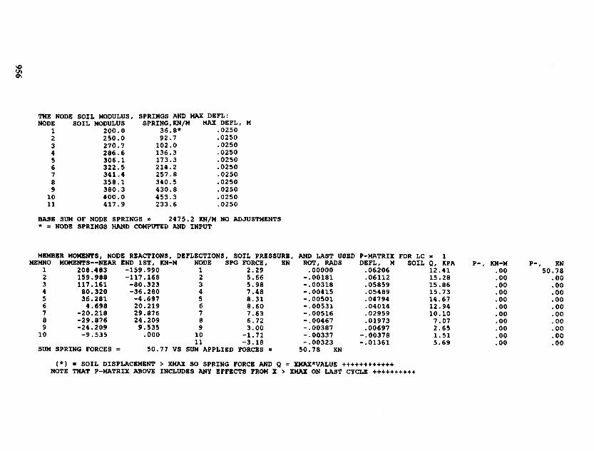
To obtain four sets of pile constants we must make two executions with respect to each prin-cipal axis of the pile. In one execution node 1 is fixed to allow rotation but no translation (dataset EX1613A.DTA); in the second execution the node is fixed to allow translation but no rotation(EX1613B.DTA). You have this sample output set as Fig. E16-13Z?. Data sets EX1613C.DTA andEX1613D.DTA are similar but with respect to the y axis.

From execution of all the data sets one can plot the Curves A and B of Fig. E16-13c. The loadswere somewhat arbitrarily chosen after making several trial runs using different values of ks sothat displacements and rotations would be large enough to produce easily identifiable data for thetextbook user.

Pile input data: HP360 X 174 Obtain Ix, bf\ Iy, d from Table A-I

E = 200000MPa

10 elements: 3 @ 1, 2 @ 1.5, 2 @ 2, and 3 @ 3 m

Kx = 200 + 50Z05

REDFAC = 0.9

Comments, (see figures on pages following)

1. Ph = 50.78 kN is plotted versus 8 = 0.06206 m for one curve with respect to the x axis.

2. The fixed-end moment (from no rotation) of 208.483 kN • m is plotted versus 8 = 0.06206 mfor a second curve, also with respect to the x axis.

3. The other two curves with respect to the x axis are obtained from executing data setEX1613A.DTA.

16-17 BUCKLING OF FULLY AND PARTIALLY EMBEDDEDPILES AND POLES

The author, using a method presented by Wang (1967) for buckling of columns of variablecross section, developed a procedure that can be used to obtain the buckling load for pileseither fully or partially embedded. The method is easier to use and considerably more ver-satile, if a computer program such as B-26 is available, than either the methods of Davissonand Robinson (1965) or those of Reddy and Valsangkar (1970). This method can be used to

My = P1= 50.78 kN • m (EX1613A • DTA)= P2 = 50.78 kN (EX 1613B • DTA)

Ix = 0.5080 x 10-3IIi4

/y = 0.1840 xlO-3m4

18.44 kN(EX1613D- DTA)

18.44 kN • m (EX1613C DTA)

NM=IONNODES = IlNP = 22JTSOIL = 1NCYC = 1NRC =l(B&D only)

Figure E16-13a

Y axis

USING H360 X 174 TO OBTAIN PILE CONST FOR EXAH 18-7—TRANSL—NO ROTAT

+++++++++++++++++ THIS OUTPUT FOR DATA FILE: EX1613B.DTA

SOLUTION FOR LATERALLY LOADED PILE—-ITTPE = 1 ++++++++++

NO OF NON-ZERO P, NNZP = 1NO OF CYCLES NCYC = 1

NO OF BOUNDARY CONDIT NZX = 1LIST BAND IF > O • O

IMBT (SI > O) s 1

NO OF NP * 22 NO OF ELEMENTS, NM = 10NO OF LOAD CASES, NLC = 1

NODE SOIL STARTS JTSOIL = 1NONLINEAR (IF > O) * O

MODULUS KCODS = 2

INERTIA, M**4

.50800E-03

.50800E-03

.50800E-03

.50800E-03

.50800B-03

.50800B-03

.50800K-03

.50800B-03

.50800E-03

.50800E-03

WIDTH

.378

.378

.378

.378

.378

.378

.378

.378

.378

.378

LENGTH

1.0001.0001.0001.5001.5002.0002.0003.0003.0003.000

NP4

4

810121416182022

NP3

3579

111315171921

NP2

2468

101214161820

NPl

13579

1113151719

MBMNO

12345678910

NX BOUNDARY CONDITIONS = 1

BOUNDARY VALUES XSPBC = .0000

THE INITIAL INPUT P-MATRIX ENTRIESNP LC P(NP,LC)2 1 50.780

MOD OF ELASTICITY E = 200000. MPA

GROUND NODE REDUCTION FACTORS FOR PILES, FACl,FAC2 = 1.00 1.00

EQUATION FOR KS = 200.0 + 50.0*Z** .50

+++++NUMBER OF NODE SPRINGS INPUT = 1

Figure E16-13fc

THE NODE SOIL MODULUS, SPRINGS AND MAX DEFL:MAX DEFL, M

.0250

.0250

.0250

.0250

.0250

.0250

.0250

.0250

.0250

.0250

.0250

SPRING,KN/M36.8*92.7102.0136.3173.3214.2257.8340.5430.8453.3233.6

SOIL MODULUS200.0250.0270.7286.6306.1322.5341.4358.1380.3400.0417.9

NODE1234567891011

BASE SUM OF NODE SPRINGS = 2475.2 KN/M NO ADJUSTMENTS* s NODE SPRINGS HAND COMPUTED AND INPUT

MEMBER MOMENTS, NODE REACTIONS, DEFLECTIONS, SOIL PRESSURE, AND LAST USED P-MATRIX FOR LC = 1P-, KN

50.78.00.00.00.00.00.00.00.00.00.00

P-, KN-M.00.00.00.00.00.00.00.00.00.00.00

SOIL Q, KPA12.4115.2815.8615.7314.6712.9410.107.072.651.515.69

DEFL, M.06206.06112.05859.05489.04794.04014.02959.01973.00697

-.00378-.01361

ROT, RADS.00000

-.00181-.00318-.00415-.00501-.00531-.00516-.00467-.00387-.00337-.00323

SPG FORCE, KN2.295.665.987.488.318.607.636.723.00

-1.71-3.18

NODE1234567891011

END 1ST, KN-M-159.990-117.168-80.323-36.280-4.69720.21929.87624.2099.535.000

MOMENTS—NEAR208.483159.988117.16180.32036.2814.698

-20.218-29.876-24.209-9.535

MEMNO12345678910

SUM SPRING FORCES = 50.77 VS SUM APPLIED FORCES = 50.78 KN

(*) = SOIL DISPLACEMENT > XMAX SO SPRING FORCE AND Q = XMAX*VALUE ++++++++++++NOTE THAT P-MATRIX ABOVE INCLUDES ANY EFFECTS FROM X > XMAX ON LAST CYCLE ++++++++++

Curve A: translation but no rotation. Curve B: rotation but no translation.

Figure E16-13c

analyze the buckling load of other pole structures such as steel power-transmission poles [seeASCE (1974) and Dewey and Kempner (1975)] or even columns of varying end conditions.

The method used in program B-26 consists in the following steps:

1. Build the ASAT matrix and obtain the ASAT inverse of the pile system for whatever theembedment geometry. It is necessary in this inverse, however, to develop the matrix suchas shown in Fig. 16-23«. All the rotation P-X are coded first, then the translation P-Xvalues. The resultant matrix can be partitioned as

In = ^i ^l *RPs A2 A3 Xs

2. From the lower right corner of the ASAT inverse (Fig. 16-236) take a new matrix calledthe D matrix (of size NXS X NX5), identifying the translation or sidesway X's as

Xs = DP5 (a)

3. Develop a "second-order string matrix" considering one node deflection at a time as Fig.16-246:

Pfs = GXsPcr (b)

4. Since Prs must be equal to Ps, substitute (b) into (a), noting that Pcr is a critical load column

matrix for which the placing order is not critical, to obtain

y axisy axis

(16-34)

Figure 16-23 (a) General coding and notation used in the pile-buckling problem. The ground line can be spec-ified at any node. Develop the ASAT, invert it, and obtain the D matrix from the location shown in (b).

This is an eigenvalue problem, which can be solved to some predetermined degree ofexactness (say, AX = 0.000000 1) by an iteration process proposed by Wang as follows:

1. Calculate the matrix product of DG (size NXS X NXS) and hold.

2. As a first approximation set the column matrix Xs(i) = 1.00.

3. Calculate a matrix X's = DGX5 using the value 1.00.

4. Normalize the X's matrix just computed by dividing all the values by the largest value.

5. Compare the differences of Xs -X's< AX and repeat steps 2 through 5 until the differencecriterion is satisfied. On the second and later cycles the current matrix values of Xs arecomputed from the values of Xs from one cycle back.

6. When the convergence criterion has been satisfied, compute the buckling load using thelargest current values in the X's and Xs matrix as

yp _ ^ s , max

c r ~~ Y^ s, max

This step is simply solving Eq. (16-34) for PCY with the left side being the current compu-tation of Xy using the preceding cycle X's on the right side.

If higher buckling modes are desired, and one should always compute at least the first twosince this method does not always give the lowest buckling load on the first mode (especially

№)

W

Part of P9

(a) Use one node deflection at atime to develop the G matrix.

(b) The G matrix for the number ofelements given in (a).

Figure 16-24 The G matrix. For partially embedded piles m will be 1 until the soil line is encountered.

if the values are close together), one may continue steps 1 through 6 using a revised DGmatrix for step 1 obtained from the following matrix operation:

{DG}/+, = {DG}/ - YLYAXs{GXs}T)i (16-35)

where / identifies the current mode and / + 1 is the next higher mode. For proof of the validity

Figure 16-25 Variation of PCT with depth of embed-ment of the pile or pole. PER = computer programvariable used by the author relating the assumed amountof Pcr at the point. KPER = computer variable to spec-ify type of skin resistance reduction as shown.

of Eq. (16-35) see Wang (1967). The values of PCT and X are obtained as the values of the ithbuckling mode.

Any variation of skin resistance to reduce Pcr, as illustrated in Fig. 16-25 to develop thestring matrix, can be used. Note that no skin resistance is used in developing the ASA andcorresponding D matrix since the assumption of small values of rotation and translation forvertical piles does not produce any skin-resistance effect. Note also that the lateral soil resis-tance effect is included only in the ASAT matrix and not in the G matrix.

This solution can be readily compared with the theoretical solutions by applying one largesoil spring at the top and bottom of the pile and no intermediate values (i.e., the pile becomesa beam column). It is possible to use a method (similar to that in your included computerprogram B-5) of zeroing boundary conditions, except that this will not work for the case of afully embedded pile with top and bottom both specified zero. Satisfactory results can usuallybe obtained with 8 to 15 finite elements.

Example 16-14. To illustrate pile buckling and the effect of soil on buckling of piles, the followingexample will be presented. Its solution requires use of program FADPILB(B-26), but you can see how buckling loads are affected by the soil from careful study of theexample.

Given. A 254-mm diam X 6.35-mm wall (10 X 0.25 in.) pipe pile that is 12 m in length. It isembedded 5 m in an extremely soft soil (average qu for full depth is only 10 kPa) with the pointon rock as shown in Fig. E16-14a. We would like to estimate the buckling load. Assume the pointcarries 50 percent of the buckling load (side friction carries a significant amount of the load of anypile in any soil—even though this is a point-bearing design). Assume further that the side frictiondistribution is parabolic (KPER = 2) as shown in Fig. 16-23. The first soil spring is reduced 25percent for driving damage.

Solution. First draw a sketch and locate the pile nodes. Note the P-X coding here is automaticallydone as in Fig. 16-23. That is, the rotation P-X values are numbered first, then the translation P-Xvalues. The program will also compute the moment of inertia of round solid, round pipe, tapered,and square piles so all you have to input (in this case) is the diameter and wall thickness.

We will have to input ks, and we will use Eq. (16-26&) and not use the Nq-term, giving

(rounded)

Node number

Pipe pileD= 10" or 254 mmtw = 0.25"or 6.35 mm

6.35 mm

JTSOIL

NM =14NP = 30

Soft clay: qu = 10 kPaAverage for full 5 m of embedment

KPER = 2

Rock

Figure E16-14a

The resulting computer output is shown on Fig. E16-14&. The Euler load shown is for a columnfixed at the ground line (making the effective column length 14 m). The Euler equation used is

p _ "'Elcr " kU

where k = 1 for members pinned on each end; = 2 for members fixed on one end; = 0.5 formembers fixed on both ends

L = length of column or member

Other terms have been previously defined.The program uses JTSOIL; when it is 1 (fully embedded pile) the Euler critical load is computed

for a column pinned at each end. Of course, if ks = 0 the program inputs lateral node springs AT, = 0so it is actually a column pinned at each end.

The program allows the user to specify boundary cases of fixing one or more nodes, however, inthe case of columns one of the nodes should be fixed by inputting a very large spring.

An alternate Euler load for this example would be for a column that is fixed on one end but 12 min length (effective length = 24 m). Inspection of the Euler load of 381.7 kN versus the computedbuckling (or critical) load of 198.0 kN (first mode) seems reasonable. We would expect a partially

254 MM X 6.35 MM TW 12 M L X 5 M EMBEDDED IN SOFT CLAY

NAMB OF DATA FILE USED FOR THIS EXECUTION: EX1614.DTA

DIAMETER OF ROUND SECTION « .25400 M WALL THICK « .006350 M

NO OF PILE ELEMENTS = 14NODS SOIL STARTS = 8 NO OF BUCKLING MODES REQD = 2

PERCENT POINT LOAD * 50.00 % NO OF NODES W/SPRINGS INPUT = 0GROUND LINE RBDUCT FAC = .750MODULUS OF ELASTICITY = 200000. MPA TOTAL PILE LENGTH = 12.00 M

PARABOLIC SKIN RESISTANCE REDUCTION—KPER = 2

PILE EMBEDMENT DEPTH, DBMB = 5.00 MBMBBD DEPTH SOIL MOD, KS = 3120.000 + .000Z**1.000 KN/M**3

BULBR BUCKLING LOAD = 381.7 KNBASBD ON AVERAGE I = .000038 M**4

LENGTH (OR L ABOVE GROUND) USED = 7.00 M

MBMNO NPl NP2 NP3 NP4 BLBM L WIDTH I, M**4 NODE SOIL MOD SOIL SPRNG ELEM FRIC1 1 2 16 17 1.000 .000 .37900E-04 1 .0 .0 1.0002 2 3 17 18 1.000 .000 .37900B-04 2 .0 .0 1.0003 3 4 18 19 1.000 .000 .37900E-04 3 .0 .0 1.0004 4 5 19 20 1.000 .000 .37900B-04 4 .0 .0 1.0005 5 6 20 21 1.000 .000 .37900E-04 5 .0 .0 1.0006 6 7 21 22 1.000 .000 .37900B-04 6 .0 .0 1.0007 7 8 22 23 1.000 .000 .37900E-04 7 .0 .0 1.0008 8 9 23 24 .500 .254 .379008-04 8 3120.0 148.6$ 1.0009 9 10 24 25 .500 .254 .37900B-04 9 3120.0 396.2 .995

10 10 11 25 26 .500 .254 .37900B-04 10 3120.0 396.2 .98011 11 12 26 27 .500 .254 .37900E-04 11 3120.0 396.2 .95512 12 13 27 28 1.000 .254 .37900E-04 12 3120.0 594.4 .92013 13 14 28 29 1.000 .254 .37900E-04 13 3120.0 792.5 .82014 14 15 29 30 1.000 .254 .37900B-04 14 3120.0 792.5 .680

15 3120.0 396.2 .500$ = NODE SPRING RBDUCED BY FAC = .750

THE BUCKLING MODE SHOWN ON OUTPUT IS USED AS A COUNTER—INSPECTIONOF THE UNIT DEFLECTIONS WILL GIVE THE CURRENT BUCKLING MODE

THB BUCKLING LOAD 18 198.0 KN FOR MODE 1 AFTER 8 ITERATIONS

TKB BUCKLING LOAD IS 1712.1 KN FOR MODE 2 AFTBR 19 ITERATIONS

NODE DISPLACEMENTS—MAXIMUM OF 3 OUTPUTMODE NO * 1 2NODB ACTUAL NORMALIZED ACTUAL NORMALIZED

1 .00505 1.00000 .00043 .518302 .00424 .83892 .00054 .741093 .00344 .68203 .00062 .914524 .00269 .53341 .00065 1.000005 .00200 .39693 .00062 .978126 .00139 .27613 .00053 .852917 .00088 .17416 .00040 .650998 .00047 .09366 .00025 .415779 .00031 .06211 .00018 .3014610 .00018 .03639 .00012 .1967511 .00008 .01605 .00006 .1047212 .00000 .00038 .00002 .0263813 -.00010 -.02046 -.00006 -.0934514 -.00017 -.03315 -.00011 -.1797115 -.00022 -.04303 -.00015 -.25211

Figure EU-Ub

embedded pile in a very soft soil not to have a buckling load as large as the Euler load of the free-standing part fixed on one end. The computed buckling load of 198 kN should be larger than thatof a 12-m column fixed on only one end. This idea is left for the reader to check.

The critical buckling load of 1712.1 kN for the second mode is larger than the first mode. Thisincrease is generally the case, but if the second mode is smaller than the first, then the secondbuckling mode governs. You should always obtain two buckling modes using a program such asthis.

////

PROBLEMS

Few answers are provided since a major part of pile design is selection of parameters. When param-eters are provided all one does is solve a given equation.

16-1. A 460-mm diameter pipe pile is driven closed-end 15 m into a cohesionless soil with an esti-mated <f> angle of 34°. The soil has a yWet = 16.50 kN/m3 and y' = 8.60 kN/m3. The GWT is6 m below the ground surface. Estimate the ultimate pile capacity P11 using the /3 method andfriction angle 8 = 22°.

Answer: P14 « 510 kN (using K = 1.5KO)

16-2. A H P 3 6 0 X 152 pile is driven into a cohesionless soil with a </> angle = 34°. The soil hasTwet = 17.3 kN/m 3 ; y' = 10.1 kN/m 3 and the G W T is 3 m below the ground surface. Estimatethe pile capacity P11 using a pile length of 16 m, the /3 method, and 8 = 22° soil-to-steel and26° soil-to-soil (in web zone). Use K = 1.0.

16-3. A pile is driven through a soft cohesive deposit overlying a stiff clay. The G W T is 5 m belowthe ground surface and the stiff clay is at the 8-m depth. Other data:

Soft clay Stiff clay

ywet 17.5 19.3 kN/m3

y' 9.5 10.6 kN/m3

su 50 165 kPa

Estimate the length of a 550-mm diam pile to carry an allowable load Pa = 420 kN using anSF = 4 and the A method.

Answer: L ~ 13 m16-4. Redo Problem 16-3 using an HP360 X 109 pile.

Answer: L ~ 16 to 16.5 m

16-5. A J taper Union Mono tube pile with a top diam of 457 mm and a taper of 1 : 48 and a lengthof 12.2 m is driven into a medium stiff clay deposit with an average su = 67 kPa. The pile willlater be filled with concrete. Estimate the ultimate capacity Pu using the a method and the APIvalue.

16-6. A Union Monotube F taper shell is driven into a cohesionless deposit with an average </> = 34°.The ywet = 17.8 and y' = 9.8 kN/m3, and the GWT is 5 m below the ground surface. The piletop diam = 460 mm and the taper is 1 : 48. For a length of 20 m what is the ultimate pilecapacity using Eq. (16-19)?

Figure P16-7

16-7. For the assigned boring log and pile (A, B, C, or D) of Fig. P16-7 estimate the pile capacityusing Meyerhof s or Vesic's equations for skin resistance and point capacity. These are actualboring logs that have been converted to SI.

16-8. What is the approximate ultimate pullout resistance T14 for a tension pile in a medium dense sandwith (/> ~ 36°, y = 18.2 kN/m3, and using an 800-mm diameter concrete pile with a length of5 m (and no bell)?

16-9. For the same data of Prob. 16-8 what is Tu if the diameter is only 300 mm, both without and

with a 1-m diameter bell?

16-10. Verify the skin resistance of the sand layers given on Fig. E16-7&.

16-11. Verify the skin resistance of the clay layers given on Fig. E16-7&. Recompute the a values.Also, what is the effect if you use a single 27-m layer with a = 1 instead of the three layers ofthe example?

16-12. See if you can reproduce the settlement computed and shown on the output sheets of Fig.

E16-76.

16-13. Redo Example 16-8 for Pa = 170 kN and with cs = 0.22 g-cal.

Bedrock at approx. 98'Rock

Decomposedrock

Misc. fill

Gray organicsUtRed-brownfine silty sand

Grayfinetocoarsesandandgravel

Boring logElev.

TestpileA

TestpileB Boring log

"5 5

value^55

value

TestpileC

TestpileD

Cindersglasswoodfill

Grayorganicsilt

Fine tocoarse sandand gravel

Gray-brown,sandymica schist(decomposed)

HP

360

x 10

9 pi

le

324

x 7.

9 m

m p

ipe

356

x 7.

9 m

m p

ipe

HP

360

x 10

9 pi

le

Figure P16-18

HP

310

x 79

16-14. Check the side resistance of Example 16-8 and estimate if creep will be a problem. If creep isa problem, how can you reduce its effect?

16-15. What is P11 for Fig. 16-18 if the pile perimeter = 1 . 3 m ; A £ = 2600 MN; L1 = 2 m (for allthree elements); and Ayp = 3 mm? Assume the point load Pp = 40 kN.

Answer: Pu ~ 657 kN

16-16. Do Example 16-12 for the other two load cases and, together with those given on Fig. E16-12&,make a plot of Ph versus displacement 8. Also plot the shear and moment diagrams for theassigned load case. If the Ph versus 8 plot is linear, what can be done to make it somewhatnonlinear since real plots of this type are seldom linear except near the origin?

16-17. Make a copy of data set EX1612.DTA as EX1612A.DTA and apply a lateral load of Ph = 40kN at node 1. Then make a second copy and fix node 4 against translation; make a third copyand input a zero spring at node 4. Compare the results and answer the following:

a. What external cause could produce a fixed node 4?b. What would reduce the spring at node 4 to 0?

16-18. Referring to Fig. P16-18 (see previous page), code and make an estimate of the P-A effect[i.e., solve with the horizontal load, then resolve where you input a moment (need a 2nd NZX)produced by the vertical load Pv X Atop with respect to the dredge line, continue doing this until5tOp converges within about 0.01 m]. The two initial data sets are included as HP1619.DTA andHP1619A.DTA on your program diskette.

16-19. Redo Example 16-13 using loads as follows:

jc-axis y-axisPh = My = 40 Ph = Mx = 20 kN or kN • m

Plot the results and see if there is any difference in the computed curve slopes. Explain whythere is or is not a difference.

16-20. Compute the Euler load for the pile of Example 16-14, assuming it is 14 m long and fixed at the

end bearing on rock, and compare your result with the buckling load shown on Fig. El6-142?.

16-21. Verify that the moment of inertia for the concrete base of Problem 16-22 would be input as

1.744 ft4 so that Est = 30000 ksi applies to all the pile elements. The Ec = 4000 ksi.

16-22. If you have the pile buckling program FADPILB (B-26) compute the buckling load for thetapered power transmission pole shown in Fig. P16-22. All element lengths are equal.

L= 10 ft (element lengths—use average diameter for /)

£steei = 30000 ksi Ec = 4 000 ksi

Element / in order from top down:

0.07, 0.095, 0.125, 0.155, 0.190, 0.2400.295, 0.350, 0.410, 0.475, 0.550, 0.6400.735, 0.825, 1.744, 1.744

Use ks = 100 + 100Z1

Answer: PCT = 216.5 kips (requires program B-26)

12-sided polygon

Drilledcone. ftg.

Figure P16-22