156 - understanding dynamic random analyses
TRANSCRIPT

8/13/2019 156 - Understanding Dynamic Random Analyses
http://slidepdf.com/reader/full/156-understanding-dynamic-random-analyses 1/20
Dynamic Analyses Understanding Dynamic Random Analyses – Lecture
UnderstandingDynamicRandomAnalyses.mp3
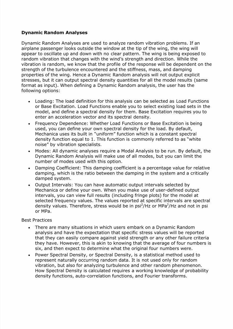
Understanding Dynamic Random Analyses
Dynamic Random Analyses solve random vibration problems with
input in the format of Spectral Density.
Options
Loading
Frequency Dependence
Modes
Damping Coefficient
Output Intervals
Airframe Model
Normal Stress RMS results (psi). (One σ results) Lecture Notes
8/13/2019 156 - Understanding Dynamic Random Analyses
http://slidepdf.com/reader/full/156-understanding-dynamic-random-analyses 2/20

8/13/2019 156 - Understanding Dynamic Random Analyses
http://slidepdf.com/reader/full/156-understanding-dynamic-random-analyses 3/20
From a practical perspective, there are a few things to keep in mind: The meanvalue for quantities in this kind of analysis is assumed to be zero. This meansthat the standard deviation (σ) of a quantity is equal to the root mean square(rms). The area underneath a spectral density curve will be the variance or themean square of the quantity. So if the requirements specify that the modelshould be designed based on 3σ stresses define a measure for root-meansquare of the maximum stress and multiply the output by 3.
It is also worth noting that only vector quantities of measures can be reportedin a Dynamic Random analysis. For example, a measure that calculatesdisplacement magnitude or Von Mises stress will not be valid for a DynamicRandom analysis. However, a measure that calculates displacement in the Xdirection or axial stress in the Z direction will be valid.
Understanding Dynamic Random Analyses – Demonstration UnderstandingDynamicRandomAnalyses_demo.mp4
Understanding Dynamic Random Analyses – Procedure Procedure: Understanding Dynamic Random Analyses
ScenarioCreate a Dynamic Random Analysis with tabular input.
CreateDynRandom satellite_frame.asm
Task 1. Open the Mechanica application and create a dynamic random analysis.
1. Click Applications > Mechanica.
2. Click Mechanica Analyses/Studies from the main toolbar.
Every dynamic analysis requires a modal analysis to be defined. Note that
the Modal_Analysis_4_Modes modal analysis has already been defined
for this model.
3. Click File > New Dynamic > Random... from the Analyses and Design Studiesdialog box.
4. In the name field, type Random_Vibration.
5. In the Direction area of the Dynamic Random Analysis Definition dialog box, type
386.4 in the Z field. Verify that the X and Y fields are set to 0.

8/13/2019 156 - Understanding Dynamic Random Analyses
http://slidepdf.com/reader/full/156-understanding-dynamic-random-analyses 4/20
Because Mechanica does not use “g” as a unit, you typed the value of g as
the base excitation (in in/s2).
6. In the Damping Coefficient (%) area on the Modes tab, verify that the drop-down
menu is set to For all modes and type 4 in the field below the drop-down menu.
The dialog box should now appear as shown in the figure.
This value is applied as a 4% damping coefficient.
7. Click Function to open the Functions dialog box.
8. Click New... to being creating a new function.

8/13/2019 156 - Understanding Dynamic Random Analyses
http://slidepdf.com/reader/full/156-understanding-dynamic-random-analyses 5/20
The PSD acceleration for this analysis is given by the following table:
Frequency (Hz) Acceleration PSD (g2/Hz)
20 0.0256
20–50 +6 dB/octave
50 0.16
800 0.16
800–2000 -4.5 dB/octave
2000 0.0256
9. In the Definition area of the dialog box, select Table from the drop-down menu.
10. Click Add Row, verify that the Start at field is set to 1, set the Num Rows field to
4 and click OK.
11. Populate the table as shown in the figure. Be sure to select Logarithmic and
Logarithmic for each of the drop-down menus at the bottom of the dialog box.

8/13/2019 156 - Understanding Dynamic Random Analyses
http://slidepdf.com/reader/full/156-understanding-dynamic-random-analyses 6/20
Changing to the logarithmic scale is critical because the table above
indicates that the slope for 20-50Hz and 800-2000Hz is on a logarithmic
scale. PSD function slopes defined as a specific dB/octave value are
common.
12. Click Review..., verify that the Lower Limit is set to 20 and the Upper Limit is setto 2000 and click Graph.
13. Once the graph is displayed in the Graphtool dialog box, click Format > Graph.
14. If necessary, select the Y Axis tab and select the Log Scale check box.
15. Select the X Axis tab and select the Log Scale check box.
16. Click OK to close the Graph Window Options dialog box and display the graph.
17. When you are finished reviewing the graph, click File > Exit > Done > OK > OK
to complete defining the function and return to the Dynamic Random Analysisdialog box.

8/13/2019 156 - Understanding Dynamic Random Analyses
http://slidepdf.com/reader/full/156-understanding-dynamic-random-analyses 7/20
18. Select the Output tab in the dialog box, select the Full RMS Results for
Displacements and Stresses check box, and type 20 in the Minimum Frequencyfield.
19. In the Maximum Frequency area, select the User-defined radio button and type2000 in the field as shown in the figure.
20. Click OK to complete the dynamic random analysis definition and close the dialog
box.
21. Return to the Standard Pro/ENGINEER mode by clicking Applications >Standard.
22. Click Save from the main toolbar and click OK to save the model.
23. Click File > Close Window from the main menu.
24. Click File > Erase > Not Displayed > OK to erase the model from memory.
This completes the procedure.
Understanding Dynamic Random Analyses – Exercise Exercise: Running a Dynamic Random Analysis
Objectives
After successfully completing this exercise, you will be able to:
Understand the different settings in a dynamic random analysis.
Type data presented as g2 /Hz into a dynamic random analysis.
Create valid measures for a dynamic random analysis.

8/13/2019 156 - Understanding Dynamic Random Analyses
http://slidepdf.com/reader/full/156-understanding-dynamic-random-analyses 8/20
ScenarioRandom analysis occurs in a number of applications. A satellite enclosed in a launch
vehicle is subject to random vibration during launch, as is an airplane when it encounters
turbulence or an off-road vehicle on uneven ground.
In this exercise, the wing of an aircraft will be analyzed for random vibration. The input
will be presented in a format and units common for this kind of problem. The input willalmost always be expressed in terms of base excitation, and the units for the spectraldensity of acceleration will almost always be in g2 /Hz. In addition, transition between
values at different frequencies will almost always be logarithmic.
Creating measures for a dynamic random analysis will be reviewed. Though a Dynamic
Random Analysis outputs quantities in spectral density, how to use the output to
determine confidence in the model will be examined.
The input for this model is specified by the table and graph below. Acceleration data for
dynamic random analysis is often obtained from empirical data. In addition, several large
institutions such as the US Army or NASA have public documents (for example, MIL-STD-
810) that include PSD Acceleration plots to be used for products designed for them. It isalso not uncommon for consumer products marketed as “rugged” or “heavy duty” to be
designed using the types of specifications.
Frequency
(Hz)
Acceleration
(g2 /Hz)
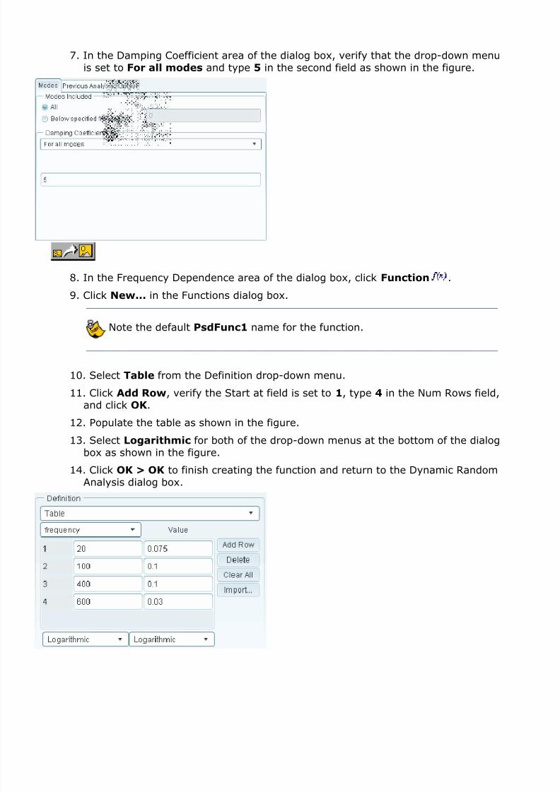
20 0.075
100 0.1
400 0.1
600 0.03
Note how the chart provided is on a log scale for both axes, and the
curve appears as straight lines. This means that when the table is
typed in Mechanica, Logarithmic interpolation has to be used.
Sometimes if a graph is not included, the slope information will be

8/13/2019 156 - Understanding Dynamic Random Analyses
http://slidepdf.com/reader/full/156-understanding-dynamic-random-analyses 9/20
included in the table in the form of dB/octave. Setting the
interpolation to Logarithmic will account for this as well.
DynRandExer wing_rgt.prt
Task 1. Open the Mechanica application and begin creating a dynamic randomevaluation.
1. Click Applications > Mechanica.
Note that the units for this model are in-lbf-s and that the model already has
a material assignment (Aluminum 6061), simulation features (4 points), and
constraints (on the inboard section of the wing).
2. Click Mechanica Analyses/Studies from the main toolbar.
Note that a modal analysis has already been created. The modal analysis
calculates the first six modes of vibration for WING_RGT.PRT.
3. In the Analyses and Design Studies dialog box, click File > New Dynamic >
Random....
4. Type Random_Vibration in the Name field.
The direction vector for base excitation has served as a scaling factor in
other dynamic analyses. In Dynamic Random analyses, the values typed into
the base excitation vector are squared and then scaled by the function
defined. So if the acceleration is reported in g2 /Hz, then the base excitation
vector should only have the value of g for that system of units, not g2. As
such, for this model the acceleration of gravity in in/s2 is 386.4.
5. Type 386.4 in the Y field as shown in the figure.
6. Select the Supports radio button in the Relative to field.
8/13/2019 156 - Understanding Dynamic Random Analyses
http://slidepdf.com/reader/full/156-understanding-dynamic-random-analyses 10/20
7. In the Damping Coefficient area of the dialog box, verify that the drop-down menu
is set to For all modes and type 5 in the second field as shown in the figure.
8. In the Frequency Dependence area of the dialog box, click Function .
9. Click New... in the Functions dialog box.
Note the default PsdFunc1 name for the function.
10. Select Table from the Definition drop-down menu.
11. Click Add Row, verify the Start at field is set to 1, type 4 in the Num Rows field,and click OK.
12. Populate the table as shown in the figure.
13. Select Logarithmic for both of the drop-down menus at the bottom of the dialog
box as shown in the figure.
14. Click OK > OK to finish creating the function and return to the Dynamic Random
Analysis dialog box.

8/13/2019 156 - Understanding Dynamic Random Analyses
http://slidepdf.com/reader/full/156-understanding-dynamic-random-analyses 11/20
15. Select the Previous Analysis tab.
Note how the previously defined Modal_Analysis_6_modes is
automatically selected at the Modal Analysis. This is due to the fact that it is
the only modal analysis currently in the working directory.
16. Select the Output tab.
17. Select the Full RMS Results for Displacements and Stresses check box as
shown in the figure.
18. Select the Mass Participation Factors check box as shown in the figure.
19. In the Output Intervals area of the dialog box, verify that the drop-down menu isset to Automatic Intervals within Range as shown in the figure.
20. Type 20 in the Minimum Frequency field as shown in the figure.
21. In the Maximum Frequency area, select the User-defined radio button and type
600 in the field as shown in the figure.
22. The dialog box should now appear as shown in the figure. Click OK to completethe Dynamic Random Analysis definition and close the dialog box.

8/13/2019 156 - Understanding Dynamic Random Analyses
http://slidepdf.com/reader/full/156-understanding-dynamic-random-analyses 12/20
Task 2. Create valid measures for the dynamic random analysis.
Measures that are valid for a dynamic random analysis have to fulfill two
requirements:
A. They must be associated with specific points on the model.
B. They must be vector quantities. (For instance acceleration magnitudeis not valid, but acceleration in the x direction is valid.)
1. Click Close in the Analysis and Design Studies dialog box.
2. Click Simulation Measure from the Mechanica toolbar and click New in the
Measures dialog box.

8/13/2019 156 - Understanding Dynamic Random Analyses
http://slidepdf.com/reader/full/156-understanding-dynamic-random-analyses 13/20
3. Type acceleration_y_tip in the Name field.
4. From the Quantity drop-down menu, select Acceleration.
5. From the Component drop-down menu, select Y.
6. Verify that the Coordinate system is set to WCS.
7. In the Spatial Evaluation area of the dialog box, select At Point from the first
drop-down menu.
8. Click Select Reference and select PNT14 from the model as shown in the
figure.
9. In the Dynamic Evaluation field, select At Each Step from the first drop-down
menu.
10. The dialog box should now appear as shown in the figure. Click OK to completethe Measure Definition and close the dialog box.

8/13/2019 156 - Understanding Dynamic Random Analyses
http://slidepdf.com/reader/full/156-understanding-dynamic-random-analyses 14/20
11. Click Copy in the Measures dialog box.
12. Select PNT14 from the model and click OK in the Multiple Measure Copy dialogbox.
13. If necessary, select the acceleration_y_tip1 and click Edit.
14. Edit the Name field to acceleration_y_tip_rms.
15. In the Dynamic Evaluation field, select RMS from the drop-down menu.
16. The dialog box should now appear as shown in the figure. Click OK to complete
the Measure Definition and close the dialog box.
17. Click Close to close the Measures dialog box.

8/13/2019 156 - Understanding Dynamic Random Analyses
http://slidepdf.com/reader/full/156-understanding-dynamic-random-analyses 15/20
Task 3. Run the dynamic random analysis and review the results.
1. Click Mechanica Analyses/Studies from the main toolbar.
2. Select the Random_Vibration analysis from the Analyses and Design Studies list
and click Start Run > Yes to start the design study.
3. Click Display Study Status once the analysis is started.
The analysis should take a few minutes to complete.
4. When the analysis is complete, review the Diagnostics and Run Status window.
Click Close to close each one when you are through reviewing it.
5. Verify that Random_Vibration is selected in the Analyses and Design Studies
dialog box and click Results to start Results mode.
6. Select Graph from the Display type drop-down menu.
7. In the Graph Ordinate (Vertical) Axis area (on the Quantity tab), select Measure
from the first drop-down menu.
8/13/2019 156 - Understanding Dynamic Random Analyses
http://slidepdf.com/reader/full/156-understanding-dynamic-random-analyses 16/20
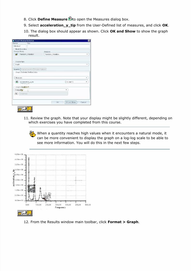
8. Click Define Measure to open the Measures dialog box.
9. Select acceleration_y_tip from the User-Defined list of measures, and click OK.
10. The dialog box should appear as shown. Click OK and Show to show the graph
result.
11. Review the graph. Note that your display might be slightly different, depending on
which exercises you have completed from this course.
When a quantity reaches high values when it encounters a natural mode, it
can be more convenient to display the graph on a log-log scale to be able to
see more information. You will do this in the next few steps.
12. From the Results window main toolbar, click Format > Graph.

8/13/2019 156 - Understanding Dynamic Random Analyses
http://slidepdf.com/reader/full/156-understanding-dynamic-random-analyses 17/20
13. Verify that the window is showing information on the Y Axis and select the Log
Scale check box in the lower-right corner of the dialog box as shown in the figure.
14. Select the X Axis tab, and select the Log Scale check box in the lower-right
corner of the dialog box as shown in the figure.
15. Click OK to view the graph in log-log format.
Note that this is the spectral density for the acceleration. The units for the y-
axis are in2 /s2Hz, not g2 /Hz
16. Click Delete Selected Definition from the Results window main toolbar.
17. From the Results Mode main toolbar, click Result Window .
18. Select Random_Vibration and click Open.
19. Type XX in the Title field.
20. Verify that the Display type drop-down menu is set to Fringe.

8/13/2019 156 - Understanding Dynamic Random Analyses
http://slidepdf.com/reader/full/156-understanding-dynamic-random-analyses 18/20
21. On the Quantity tab, select Stress from the first drop-down menu as shown in the
figure.
22. If necessary, set the Component drop-down menu on the Quantity tab to XX.
Note that there is no Von Mises stress available—it is not calculated for a
dynamic random analysis.
23. Click OK and Show to show the Fringe plot result.
24. Click Copy from the main toolbar in the Results window.
25. Edit the title field to read YY.
26. Select YY from the second drop-down menu on the Quantity tab.
27. Click OK and Show to show the Fringe plot result.
28. Click Copy from the main toolbar in the Results window.
29. Edit the title field to read ZZ.
30. Select ZZ from the second drop-down menu on the Quantity tab.
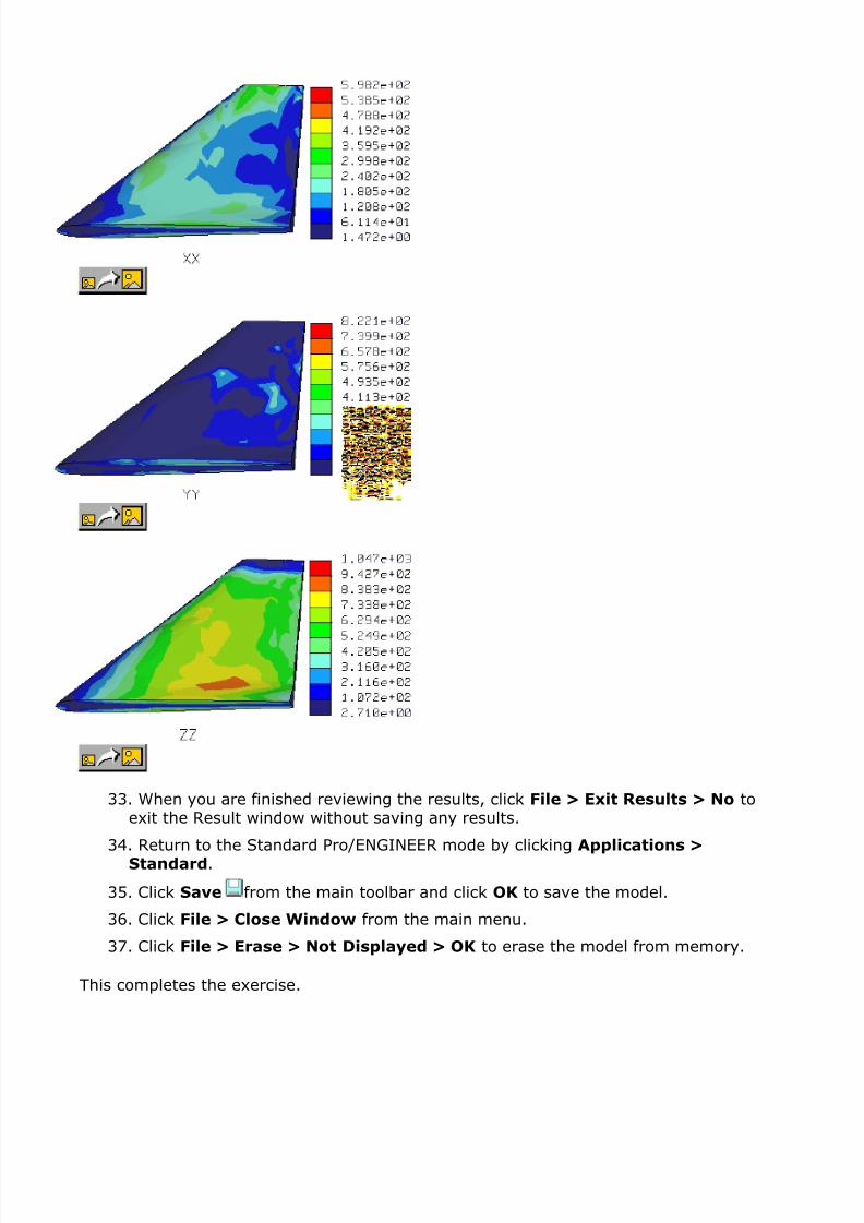
31. Click OK and Show to show the Fringe plot result.
32. Review the resulting fringe plots.
The highest of the axial stresses appears to be 1,081 psi in the Z direction.
Note that the values of stress reported here are the root mean square (RMS)
stresses, not the actual stress on the model at any point in time. It is
assumed that since the vibration is naturally occurring, it follows a normal
probability distribution function and has a mean of zero. If the mean is equal
to zero, then the root mean square is equal to the standard deviation (sigma
or σ). One way you can use this to judge results for random vibration is to
use “three sigma” results. It is believed that there is a 0.3% probability that
the value could be higher than three standard deviations. So for your stress
of 1,081 psi, the three-sigma value would be 3,243 psi. This means there is
only a 0.3% chance that the axial stress will be higher than 3,243 psi. This
is well below the yield stress for Aluminium 6061, which is 40,000 psi.
8/13/2019 156 - Understanding Dynamic Random Analyses
http://slidepdf.com/reader/full/156-understanding-dynamic-random-analyses 19/20
33. When you are finished reviewing the results, click File > Exit Results > No toexit the Result window without saving any results.
34. Return to the Standard Pro/ENGINEER mode by clicking Applications >Standard.
35. Click Save from the main toolbar and click OK to save the model.
36. Click File > Close Window from the main menu.
37. Click File > Erase > Not Displayed > OK to erase the model from memory.
This completes the exercise.

8/13/2019 156 - Understanding Dynamic Random Analyses
http://slidepdf.com/reader/full/156-understanding-dynamic-random-analyses 20/20