15 the empirical strength of the labour theory of value frances/labthvalue.pdf · 15 the empirical...

15 The Empirical Strengthof the Labour Theory ofValueAnwar M. Shaikh

INTRODUCTION’

The purpose of this chapter is to explore the theoretical and empiricalproperties of what Ricardo and Smith called natural prices, and whatMarx called prices of production. Classiml and Marxinn theories ofcompetition argue two things about such prices. First, that themobility of capital between sectors will ensure that they will act ascentres of gravity of actual market prices, over some time period thatmay be specific to each sector (Marx, 1972, pp. 174-5; Shaikh, 1984,pp. 48-9). Second, that these regulating prices are themselvesdominated by the underlying structure of production, as summarizedin the quantities of total (direct and indirect) labour time involved inthe production of the corresponding commodities. It is this doublerelation, in which prices of production act as the mediating linkbetween market prices and labour values, that we will analyze here.

At a theoretical level, it has long been argued that the behaviour ofindividual prices in the face of a changing wage share (and hencechanging profit rate) can be quite complex (Sraffa, 1963, p. 15;Schefold, 1976, p. 26; Pasinetti, 1977, pp. 84, 88-89; Parys, 1982, pp.1208-9; Bienenfeld, 1988, pp. 247-8). Yet, as well shall see, at anempirical lcvcl their bchaviour is quite regular. Moreover theseempirical regularities can be strongly linked to the underlyingstructure of labour values through a linear ‘transformation’ that isstrikingly reminiswnt nf Marr’c nwn pmcedure.

In what follows we will first formalize a Marxian model of prices ofproduction with a corresponding Marxian ‘standard commodity’ toserve as the clarifying numeraire. We will show that this price systemis theoretically capable of ‘Marx-reswitching’ (that is, of reversals inthe direction of deviations between prices and labour values). We willthen develop a powerful natural approximation to the full price

225

2 2 6 The Labour Theory of Value

system, and show that this approximation is the ‘vertically integrated>version of Marx’s own solution to the transformation problem.Lastly, using US input-output data developed by Ochoa (1984), wewill compare actual market prices to labour values, prices of pro-duction and the linear approximation mentioned above. It will beshown that various well-known propositions in both Ricarclo andMarx, concerning the underlying regulators of market prices, turn outto have strong empirical backing. In particular, measured in terms oftheir average absolute percentage deviations, prices of production arewithin 8.2 per cent of market prices, labour values are within 9.2 percent of market prices and 4.4 per cent of prices of production, and thelinear approximation is within 2 per cent of full prices of productionand 8.7 per cent of market price~.~ Lastly, we find that Marx-reswitching is quite rare (occurring only 1.7 per cent of the time), andmoreover is confined to MPPP where the price-value deviations aresmall enough to be empirically unimportant. All these results point tothe dominance of relative prices by the structure of production, andhence to the great importance of technical change in explainingmovements of relative prices over time (Pasinetti, 1981, p. 140).

MARXIAN PRICES OF PRODUCTION AND A MARXIANSTANDARD SYSTEM

Lower-case variables are vectors and scalars, and upper-case ones arematrices. Dimensionally, all row vectors are (I x n), column vectors(n x I), and matrices (n x n).

l a0 = row vector of labour coefficients (hours per dollar of output).l A = input-output coefficients matrix (dollars per dollar of output).l D = depreciation coefficients matrix (dollars per dollar of output).l K = capital coefficients matrix (dollars per dollar of output).l T = diagonal matrix of turnover times.l U = diagonal matrix of industry capacity utilization rates.0 w = wage rate.l r = rate of profit.‘P = vector of prices of production.0 v = vector of labour values.l m = vector of market prices.

Both flows and stocks, per unit output flow, enter into the definitionof unit prices of production. But whereas flow-flow coefficients such

Anwar M. Shaikh 2 2 7

as labour or material flows per unit of output may be taken to berelalivdy imsusitivc to changes in cayacity utilization (which is thepremise, for instance, of input-output analysis), the same cannot besaid of stock-flow coefficients such as capital requirements per unit ofoutput. In this case, any presumed stability of coefficients for a giventechnology must refer to the ratio of stocks to normal capacity output,or equivalently to the ratio of urilized stocks to actual output (Shaikh,1987, pp. 118-19,125-26; Dumenil and Levy, pp. 250-2). With this inmind, the total stock of capital advanced consists of the money valueof utilized tixed capital per unit of output (pKU) and the utihzedstocks of circulating capital per unit of output (PA + wao)TU, wherethe turnover times matrix T translates the flow of circulating capitalinto the corresponding stock (Ochoa, 1984, p. 79). Then Marxianprices of production will be defined by:

(15.1)

Let A1 = A -I-D, B = (I - Al)-‘, W = (K + A)UB, ~1 = cq.T.B,and v = a.3. Then from equation 15.1 we can writep = WV + rpH + r.w.al. But since the row vector al can be written asal - aoTB = uoB(B-‘TB) = v(B-‘TB) = VTI,where Tl = (B-‘T.B) = (I - AI).T(Z - AI)-‘,

P = WV i- rwvT1 + rpH ( 1 5 . 2 )

which yields

p = wv(2 + rTl)(Z - r. H)-’ ( 1 5 . 3 )

We know that the wage rate and profit rate are inversely related, sothat p =p(r) (Sraffa, 1963, ch. 3). At one limit we havew = 0, r = R = the maximum rate of protit, so from equation 15.2.

(l/R) *P(R) = ~(4 . H (15.4)

which implies that l/R is the dominant eigenvalue of H.At the other limit, w = W the maximum wage, and r = 0. Then

from equation 15.2, p(O) = WY - that is, prices are proportional tolabour values when r = 0. The Marxian standard system will bedefined by a column vector Xs, such that


(l/R) . Xs = H . Xs ( 1 5 . 5 )

so that Xs is the dominant eigenvector of H.Letting X = the gross output vector in the actual system, we scale

the output vector of the standard system in such a way that thestandard sum of values = the actual sum of values.

v.xs= v.x ( 1 5 . 6 )

We scale the price system such that (for all r) the standardprices equals the standard (and actual) sum of values.

sum of

p(r) . xs = v . xs ( 1 5 . 7 )

Thir p-ire nnmnli~ntinn is equivalent to expressing all mnney valuesin the standard labour value of money, v.Xs/p.Xs. Alternatively, sinceat r = 0, equation 15.2 yields p(0) = W,v, where W = the maximummoney wage, the normalization p(r).% = v.Xs (for all r) impliesW = 1 - that is, that the maximum money wage is the numeraire.To define the wage-profit curve implicit in the general price system,from equations 15.2, 15.5 and 15.7 we write

pXs=wv(Z+r.Tl)Xs+r.p.H.Xs

By construct ion, H. Xs = (I/R)Xs, and pXs = vXs. Definets = (v . Tl . Xs)/(v . Xs) = the average turnover time in the standardsystem. Then we get I = w(1 + r.ts) + (r/R), so the Marxian standardwage-profit curve is given by

w = (1 - [r/R])( 1 + r . ts) ( 1 5 . 8 )

Once the standard commodity is selected as the numeraire (equations15.67), then what was previously the money wage, w, is now the wagedefined in terms of the standard labour value of money, or equiva-lently as a fraction of the maximum money wage, W.

Note that the Marxian standard wage-profit curve is not linear. Ifwe had constructed our price system as a Sraffran one with wages paidat the end, so that wages advanced, w.a did not appear as part of totalcapital advanced in equation 15.1, then equations 15.2 and 15.8 wouldreduce to the Sraffian expressions shown below, and the wage relationwould be linear.

Anwar A4. Shaikh 2 2 9

p=wv+rpH (152a)

w = 1 - (r/R) (15.&z)

Even so the standard commodity, Xs, we have defined here is notgGuclally ~IIG same as a SraIliian one. I1 can be shown that even whenthe wageprofit curve is linear, there are in fact two standard com-modities that will do the trick (see Appendix 15.1).

MARX-RESWITCHING

In Marxian analysis the direction of individual price-value deviationsis quite important, since it determines transfers of surplus valuebetween sectors and regions, and between nations on a world scale(Shaikh and Tonak, 1994, pp. 347). Yet one of the properties of ageneral price of production system is that relative prices can switchdirection as the rate of profit varies (Sraffa, 1963, pp. 37-8). I willrefer to this phenomenon as ‘Marx-reswitching’.

Consider the simple case of a pure circulating capital model, in whichwe abstract from fixed capital so that K = 0 and D = 0, and fromturnover time so that ti = 1 for all i and hence T = 1. Then the Marxianprice system and wage curve in Equations 15.1, 15.3 and 15.8 reduce to

p=w(l+r)v+rpH

where now H = A(1 - A)-*

(152b)

w( 1 + r) = 1 - (r/R) (15.8b)

Then for a0 = (0.193 3.562 0.616) and

0.05 0.768 0.020 . 1 6 90 . 1 0 1

we get R = 1.294 and v = (0.845 4.211 1.494). Figure 15.1 shows thatthe standard price-value ratio, pv3(r), mltnthy rises above 1 and thenfalls below it, signalling a Marx-switch at roughly T = 1.1.

The preceding numerical example demonstrates that Marx-reswitching is possible. Dut it ncitlm establishr;s lhe condilions under

2 3 0 The Labour Theory o f Value

‘7--l1.02

Ph (4

1

II24

-_-___-_-_--_

0. 9 80 0 . 5

Figure 15.1 Standard price-value ratio, Sector 3

which it occurs, nor its likelihood. Although we WUIIU~ yu~suc thepoint here, further analysis suggests that when such instances occur,they do so only when an individual commodity’s capital compositionis ‘close’ to the standard one, so that its price of production is closeenough to its labour value for ‘Wicksell’ effects (the effects of generalprice-value deviations on the money value of capital advanced) tohave a significant influence. This is evidently the case in the precedingnumerical example. More importantly, we shall see that it is also thecase in every one of the (rare) empirically observed instances ofreswitching (only six cases out of 355 over all years) in the US data.If true, it implies that Marx-reswitching is unimportant at anempirical level: first, because it is rare; and second, because even whenit does occur, it does so only when the transfer of value involved isnegligible because the pricevalue deviation is small.

APPROXIMATING PRICES OF PKUUUC LION

A price system of the form in equations 15.2 and 15.8 (or indeed of theSraffian equivalent in equations 15.2a and 15.8b) is in principlecapable of very complex behaviour as far as individual prices areconcerned. But there is an underlying core which is quite simple. Tosee this, WC begin by expressing equation 15.2 in terms of a singleprice, pi of the ith sector.

pi = wvi + I. ki(r) ( 1 5 . 9 )

Anwar M. Shaikh 231

where kl (r) = W( Ti + p(r).H’. T; and Hi are the ith columns of theturnover matrix Ti and the vertically integrated capital coefficients mat-rix H, respectively, so the term Ki(r) represents the money value of thevertically integrated capital advanced per unit output of the ith sector.

We know from Sraffa (1963) that as r -+ R, in every industry i the(money value of the) output-capital ratio, qi approaches the standardoutput-capital ratio, qs = R. This can be derived directly fromequation 15.4. Note that this standard ratio R, which is the verticallyintegrated output-capital ratio of every industry at r = R, is also thelabour value of vertically integrated output-capital of the standardsystem. To see this, multiply equation 15.5 on both sides by the labourvalue vector, v, to get v.Xs/v.H.Xs = A = qs

At the other limit, when r = 0 and the standard wage w = 1, we getp = v (standard prices equal labour values) and the ith sector’soutput-capital ratio becomes qai = vi/(H’ + 7’i), which is reciprocalof the labour value of the sector’s vertically integrated technicalcomposition of capital (that is, the ratio of the total labour timerequired for the production of commodity i to the total labour timematerialized in the total capital inputs for this same commodity).’

We see therefore that for 0 < r < R the output-capital ratio q1 (r) ofevery industry must lie between its own labour value output-capitalratio, qoi and the common standard labour v&e output-capital ratioqs. With this in mind, we turn to a simple approximation of the pricesystem. The general system of equation 15.2 can be expressed as

p=wv+r.wvTl+ rpH = (wv[I I- r. Tl] + I. vH) + r@ - v)H(15.10)

In this expression, the first term on the right-hand side(wj1 f r.Tl] f r.vH) represents the component of prices of productionthat arises when constant capital (fixed capital and inventories) isvalued at its labour value, while the remaining term represents thefurther effects of price-value deviations on the value of capital stocks.The first term is therefore the vertically integrated equivalent ofMarx’s transformation procedure, as presented in volume III ofCapital. We may call it the Marx component of prices of production.The second term, on the other hand, may called the Wicksell-Sraffacomponent (Schefold, 1976, p. 23). On the assumption that thissecond term is small (which we will test shortly), we may approximateprice of production via the Marx component alone:


p’(r) = WV + r(wTl + H) = (w[Z + r. T,] + r . H)v (15.11)

Equation 15.11 implies a corresponding approximation for theoutput-capital ratio. Here the approximate unit capital advanced isq(r) = wv(T~)’ + vHi, so that the output-capital ratio is

d(r) = pi/$ = (wvi + I. ki)/< = (wv~/~wT~ + H’]) + r ( 1 5 . 1 2 )

This latter approximation4 yields the sectoral labour value ratioqoi = vi/(H’ + T:) w hen r = 0 and w = 1, and yields the standardlabour value ratio (standard outputaapital ratio) qs = R whenr = R and w = 0. In other words, the simple approximation to pricesof production in equation 15.11 is equivalent to approximating eachsector’s output-capital ratio in terms of components that depend onlyon labour values, and in such a way that each sectoral output-capitalratio approximntinn is pvnct at the two endpoints r = 0 and T - R.’

The linear price approximation in equation 15.11 is a verticallyintegrated version of Marx’s own transformation procedure. It is bothanalytically simple and, as we shall see, empirically powerful.However, before we proceed to the empirical analysis, it is worthnoting that quadratic and higher approximations of the general pricesystem of equation 15.2 can be easily developed. In effect, the the linearapproximation p’(r) was created by sustituting the value vector v forthe price vector p(r) on the right-hand side of equation 15.2, whichamounts to ignoring the (Wicksell) effects of price-value deviations onthe vertically integrated capital stock. A quadratic approximation canin turn be created by substituting p’(r) for p(r), which amounts toignoring the effects of the errors in the linear approximation on thevertically integrated capital stock, and so on.6 Although the quadraticapproximation has little improvement to offer for US data, it will turnout to be useful in our discussion below of empirical applicationspure circulating capital model Marzi and VaIli, 1977.

EMPIRICAL RESULTS: MARKET PRICES, LABOUR VALUESAND PRICES OF PRODUCTION

The empirical calculations presented here are based on the datadeveloped by Whoa (1984), covering the input-output years 1947,1958, 1963, 1967 and 1972. Work is underway to extend the results tothe years 1977, 1982 and 1987 (the last available input-output year).Further details are in Appendix 15.2.

Anwar M. Shaikh 233

Since most data patterns are similar across all the input-outputyears, we will generally use the 1972 data to illustrate them. Anyexceptional patterns will then be separately identified. It is useful tonote at this juncture that because input-output tables are cast in termsof aggregated industries, there is no natural measure of ‘output’ for agiven sector. One must pick a level such as (say) $100 worth of outputin each sector, which means that the market price for this output is$100 for each sector. Such a procedure poses no real problems for thecalculation of unit labour values or prices of production, but whencomparing vectors it does require one to distinguish between ‘clo-seness of tit’ in the sense of the deviation (distance) between themfrom the correlation between them (Ochoa, 1984, pp. 121-33;Petrovic, 1987, pp. 207-8). General measures of the proportionaldeviation between two vectors, such as the mean square error (MSE),root mean square error (RMSE), mean absolute deviation (MAD)and mean absolute weighted deviation (MAWD) are all line, and giveessentially similar results for this data. But the correlation coefticientR, or the R2 of a simple linear regression, are not meaningful in thiscase because (by construction) market prices show no VariatiOn, and

hence will show no covariation with the other vectors. In what followswe will therefore select the mean absolute weighted (proportional)deviation (MAWD), caoh motor’s weight b&g equal to its shnrc inthe labour or money value of total gross output. For two vectors withcomponents xi, yi, and with weights zi, mean absolute weighteddeviation (MAWl3) = !C(Iyi - TC~/Z~)/Y!Y~~~

MarketRate of

Labour Values a n d IViCeS of Product ion at the observed

For each input-output year, total labour times’ v = ao(l - AI)-’ arecalculated directly. Using the actual (uniform) rate of profit in eachinput-output year (Ochoa, 1984; p. 214), we calculate standard pricesof production (prices of production in terms of the standard com-modity) from equations 15.2 and 15.8 Since we have only averageannual rates of capacity utilization u for the economy as a whole(Shaikh, 1987), we do not use them when calculating individual pricesof production. We do use them, however, when subsequently com-paring the time trend of the observed actual and maximum profit rater and R, respectively, to those of the normal-capacity rates r, = r/uand R, = R/U.’

234 The Labour Theory of V&c

Standard prices of production are defined by the scalingP(F) Xs c 1’. .Y for all r (since this d~fin~c the standard commodityas the numeraire), so they are implicitly in the same units as labourvalues (which they equal at I = 0). They can therefore be directlycompared to labour values. To make market prices comparable toboth, we rescale market prices to units of labour time by multiplyingthe market price vector, m by the standard value of money= m . Xs/v . XT. This makes all three vectors have the same sum ofprices, and hence the same average level, wluch racrhtates directcomparisons of their levels. It does not, of course, change relativemarket prices in any way.

In all years, both total labour times ami pric;F;s of productionare quite close to market prices. Table 15.1 summarizes the meanaverage percentage deviation (MAWD) between various pairs ofw&tu1s.

Table 15.1 establishes that both labour values and prices of pro-duction are quite close to market prices, with average percentagedeviations of 9 per cent for the former and 8 per cent for the latter.It also establishes that labour values and prices of production arecloser to each other than to market prices, with an average deviationof only 4.4 per cent between the two.

Table 15.1 Average percen tage dev ia t ions (MAWD), (resealed) m a r k e tp r i ces , I abour va lues and p r i ces o f p roduc t ion a t obse rved ra t e s o f p ro f i t

1947 1958 1963 1967 1972 AveraRe

Labour value vs 0.105 0 . 0 9 0 0.092 0.102 0.071 0.092m a r k e t p r i c e

Pr ice o f p roduc t ion 0 .114 0 . 0 7 5 0 . 0 7 6 0 . 0 8 4 0 . 0 6 3 0 . 0 8 2vs marke t p r i ce

Labour va lue vs 0 . 0 5 6 0 . 0 3 8 0 . 0 3 8 0 . 0 4 8 0 . 0 3 8 0.044pr i ce o f p roduc t ion

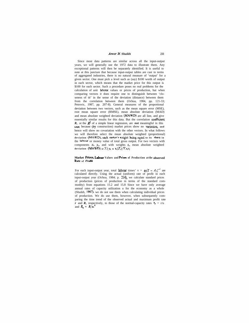
Figure 15.2 illustrates the strong empirical connection betweenlabour values and market prices for 1972, with the horizontal axisrepresenting the total market value of standard sectoral outputs(ms&, where mg = observed market prrces rni resealed in themanner discussed above) and the vertical axis representing the corre-sponding total labour values. A 45” line is also shown for purposes ofvisual reference.


v,xs,

ms, Xs,

Figure 15.2 T o t a l labour va lues v s t o t a l (resealed) marke t p r i ce s , 1972( log sca les )

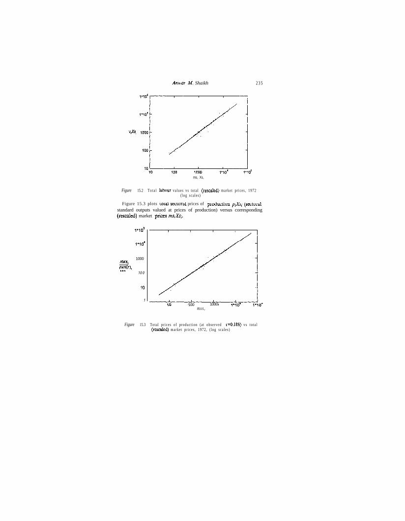
Figure 15.3 plots 10Ld secloral prices of ploducliou YiXSi (wxtulalstandard outputs valued at prices of production) versus corresponding(resealed) market prk msiXSi.

IflO

1*10'

10003PXW,***

1 0 0

IO

1100 1000

mxs ,

Figure 15.3 To ta l p r i ces o f p roduc t ion ( a t obse rved r=0.188) v s t o t a l(resealed) marke t p r i ce s , 1972 , ( l og s ca l e s )


Calculating Marxian Standard Prices of Production as Functions of theRate of Profit

The next set of results pertain to the behaviour of standard prices ofproduction as the rate of profit varies between r = 0 and r = R.Four things immediately stand out. First, in all years the relationshipbetween the rate of profit and individual prices of production isalmost invariably linear. Second, instances of Marx-reswitching arevery rare (six cases out of 355 total prices in all the years). Andthird, the previously developed linear approximation to prices ofproduction, which represents a vertically integrated version ofMarx’s own ‘transformation procedure’, performs exceedingly well:the average deviation over all years between the approximation andfill prices of production is on the order of 2 per cent! And fourth, inrelation to market prices, the linear approximation performs slightlybetter than full prices of production in one year and slightly worse inthe others, with an average deviation of only 8.7 per cent (comparedwith 8.2 per cent for full prices of production in relation to marketprices).

Figure 15.4 displays the movements of standard price of pro-duction-labour value ratios PvT(r)i as the ratio x(r) = r/R variesbetween 0 and 1 (that is, as r varies between 0 and R) for 1972. Thestriking linearity of these patterns holds in all other years. In readingthe various graphs, it is important to note that their vertical scalesvary. Also of interest are the two imtances of Marx-reswitching thatoccur in sectors 56 (aircrafts and parts) and sector 60 (miscellaneousmanufacturing). Figure 15.5 and 15.6 present a close-up of thisphenomenon. Over all years, there are only six cases of reswitchingout of 355 prices series, and as hypothesized, in each case the switchesin the direction of standard price-value deviations occur only whenthe price is itself very close to value throughout the range of the rateof profit.

Since labour values and market prices are given in any input-outputyear, the essentially linear structure of standard prices of productionwith respect to the rare of profit implies that the average deviationbetween prices of production and labour values (and market prices)increases more or less monotically with the rate of profit r. It is ofinterest, however, to note that the range of these deviations is quitesmall: even at the maximum rate of profit, price-value deviationsaverage only 12.8 per cent over all years. Table 15.2 reports theseupper limits in each year.


Table 15.2 Average deviations of standard prices of production from labourvalues, at r = R-

1947 19.58 1963 1967 1972 Overall average

A v e r a g e deviation 0.193 0.119 0.111 0.115 0.102 0.128atr=R

Testing the Linear Approximation to Full Pricea of Productiou

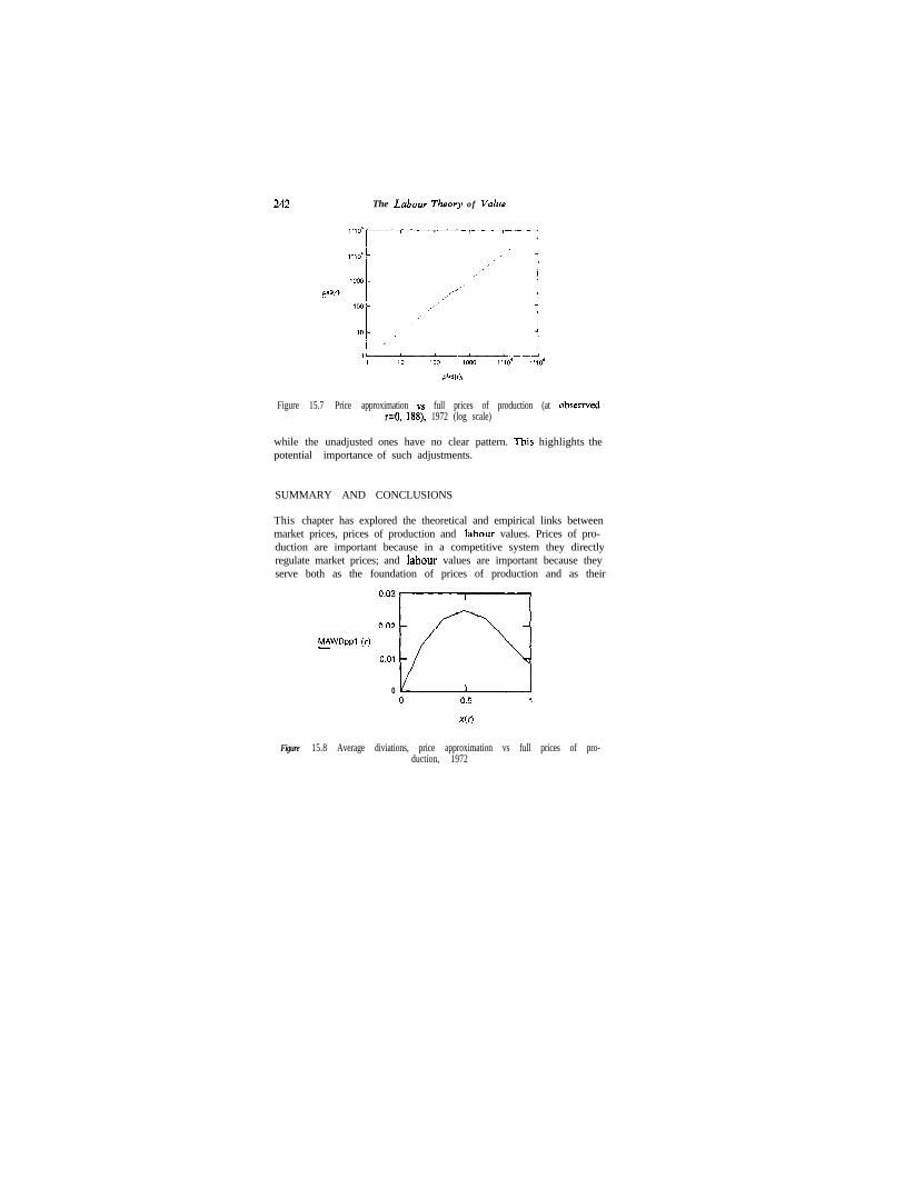
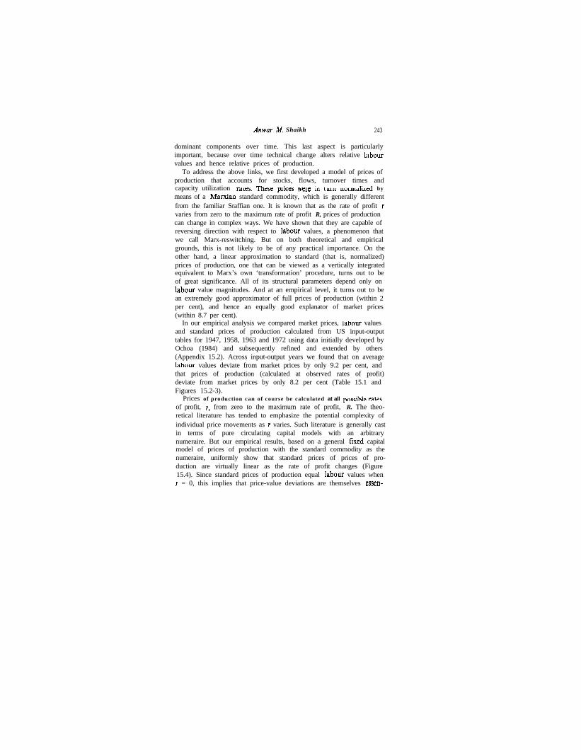
We turn next to the relation between full standard prices of pro-duction and the linear approximation developed in equation 15.11.As noted earlier, this approximation, which represents a verticallyintegrated version of Marx’s own transformation procedure,performs extremely well as a predictor of full prices of production(with an overall average deviation of only 2 per cent) and as apredictor of market prices (with an average deviation of 8.7 per cent).Figure 15.7 illustrates for 1972 a (typical) scatter between the twosets of prices, which are so close that the scatter looks like astraight line even though there is no reference line on this graph.Figure 15.8 plots the path of the corresponding average deviationas x(r) F r/R varies. Note that the largest deviation is ouly 2.5 pmcent, and that the endpoint at r = R is only 1.5 per cent. This toois typical.

Table 15.3 Actual and normal-capacity rates of profit

I 9 4 7 1958 1963 1967 1972__~

Actual profit rate, r 0.247 0.179 0.212 0.233 0.188Maximum prof i t ra te , R 0.806 0.700 0.739 0.748 0.670Capacity utilization, u 0.876 0.819 0.995 1.129 1.088Adjusted actual profit rate, r,, 0.281 0.219 0.213 0.207 0.173A d j u s t e d maximum profi t ra te R, 0.921 0 .842 0 .743 0 .663 0 .616

Finally, as noted earlier, Marx’s analysis of the trends of actual andmaximum rates of profit abstracts from the fluctuations produced bycyclical and conjunctural phenomena. As such, the relevant empiricalmeasures are normal (capacity adjusted) rates, not observed ones. Inthis regard it is interesting to see what a difference it makes to theperceived trends of P and R when one adjusts for capacity utilization.Table 15.3 presents the observed rates of profit r (Ochoa, 1984, p. 214).

2 3 8 The Labour Theory of V&c

Standard price-value ratios(Marxian prices of production)


0 0 . 5 1

40

Standard price-value ratios(Marxran prices ot production)


1.4 -

PvY~),,

._._.__ . . .. ’ . .

--. ,0.9 _

0 0 . 6 1

x(r)

pvT(r),1.5

PvTVh

PvYO,,

pvT(r),, . _. .

0.5 -0 0 . 5 1

x(r)

PvTVh- 2

pvVLo.._...

PVTW,,- 1.5

wT(r),,-

PvW,,-

1

PfW,,. . . . .

Figure 15.4 The behaviour of standard price-value ratios as x(r) = r/Rvar ies , 1972

P~TW,,

~vT(rh. . .._.

~vT(r),,

NW,,

pvT(r),,

PvW,,

dnwnv M. Shaikh

Figure 15.4 continued

239


“I’

2.5

2

1.5

0.5 ow1x(r)Standard price-value ratios Standard price-value ratios

(Marxian prices of production) (Marxian prices of production)

P~TW,,__..__ 0.95 -

0.9 I

Standard price-value ratios(Marxian prices of production)1.8

NV),,-

wTM,,1.6

PvW) 33-

PVV-)H 1.4-

t-Wr)35-

p~T(r),'.~. . .._.

0 0.5 1x(r)

PvW,,-

PvW,,~

~vT(r),,

P~TW,,

0 0 . 5 1A(1)

0 0.5 1x0)


Figure 15.4 continued

Standard price-value ratios Standard price-value ratios(Marxian prices of production) (Manian prices of production)

1 . 1

1.05P”W,S-P”W),-..___

1P”W,,-

PvW,,- 0 . 9 5

P” W,,-

P’W-), 9. .._..

0.85 L0

P”TW,,-

P”W,

PvV),-

P”W,-

P”TV),-

PVW,

I

. ’

/y” -

<.. ---__* .

‘\ .-..‘\

- . .

‘\1. -

\1 I

0.5x(r)

Standard price-value mtios(Manian prices of production)

31--13-

/

2 /

I_;_

’ /’’ /’

1.5 *‘,’. ,/-‘/,.’

1I ‘*,_______.l..-.-

1.2 I

1.15 -P”TW,,

. . .PvTV),,

vQ

- 0 . 9 5 - \’\’ \

P” TV), 1 ,..---- 0.9 - i

0.85 I0 0.5 1

x(d


I.511

PvW,,

P”V),. . . . . .

P”W,,

P”W,O

/// /

/ /’,/0-

/’

’ .Y_..,

;:-:

. . . _

.5

P”W),,__

0-0 0.5 1

XV)

0.5 ,L---L--l0.5 1x(r)

>Anwar M. Shaik 241

1 . 0 4

1 . 0 2

PW),,-P~T(&,- - -

0 . 9 6

0 0 . 5 1

x(r)

Figure 15 .5 Price-value reswitching, Sectors 56 and 60, 1972

Figure 15.6 Price-value reswitching, Sectors 56 and 60, 1972

our own calculations for the maximum rate of profit R and data oncapacity utilization rates (Shaikh, 1987, Appendix B), which is thenused to calculate normal capacity rates of profit, and r, = r/u, asdiscussed previously. Note the adjusted rates exhibit a falling trend,

212 The Labour Theory of Value

Figure 15.7 Price approximation vs full prices of production (at obserrvedr=O. 188), 1972 (log scale)

while the unadjusted ones have no clear pattern.potential importance of such adjustments.

This highlights the

SUMMARY AND CONCLUSIONS

This chapter has explored the theoretical and empirical links betweenmarket prices, prices of production and labour values. Prices of pro-duction are important because in a competitive system they directlyregulate market prices; and labour values are important because theyserve both as the foundation of prices of production and as their

MAWDppl-

0

Figure 15.8 Average diviations, price approximation vs full prices of pro-duction, 1972

Anwar M. Shaikh 243

dominant components over time. This last aspect is particularlyimportant, because over time technical change alters relative labourvalues and hence relative prices of production.

To address the above links, we first developed a model of prices ofproduction that accounts for stocks, flows, turnover times andcapacity utilization rdles. Toast: priMs wtxt: iu ~LIIII uwlulalizcd bymeans of a Marxian standard commodity, which is generally differentfrom the familiar Sraffian one. It is known that as the rate of profit rvaries from zero to the maximum rate of profit R, prices of productioncan change in complex ways. We have shown that they are capable ofreversing direction with respect to labour values, a phenomenon thatwe call Marx-reswitching. But on both theoretical and empiricalgrounds, this is not likely to be of any practical importance. On theother hand, a linear approximation to standard (that is, normalized)prices of production, one that can be viewed as a vertically integratedequivalent to Marx’s own ‘transformation’ procedure, turns out to beof great significance. All of its structural parameters depend only onlabour value magnitudes. And at an empirical level, it turns out to bean extremely good approximator of full prices of production (within 2per cent), and hence an equally good explanator of market prices(within 8.7 per cent).

In our empirical analysis we compared market prices, labour valuesand standard prices of production calculated from US input-outputtables for 1947, 1958, 1963 and 1972 using data initially developed byOchoa (1984) and subsequently refined and extended by others(Appendix 15.2). Across input-output years we found that on averagelabour values deviate from market prices by only 9.2 per cent, andthat prices of production (calculated at observed rates of profit)deviate from market prices by only 8.2 per cent (Table 15.1 andFigures 15.2-3).

Prices of production can of course be calculated at all pnmihle rstcsof profit, I, from zero to the maximum rate of profit, R. The theo-retical literature has tended to emphasize the potential complexity ofindividual price movements as r varies. Such literature is generally castin terms of pure circulating capital models with an arbitrarynumeraire. But our empirical results, based on a general fixed capitalmodel of prices of production with the standard commodity as thenumeraire, uniformly show that standard prices of prices of pro-duction are virtually linear as the rate of profit changes (Figure15.4). Since standard prices of production equal labour values whenI = 0, this implies that price-value deviations are themselves essen-


tially linear functions of the rate of profit. For this reason, thelinear price approximation developed in this chapter performsextremely well over all ranges of r and over all input-output years,deviating on average from full prices of production by only 2 per cent(Figures 15.6-7) and from market prices by only 8.7 per cent (asuppusd to 8.2 per cent for full prices of production relative to marketprices).

What explains the linearity of prices of production over all rates ofprofit? It is certainly not because prices of production are close tolabour values, as Figure 15.4 makes clear: in 1972 the coefficient ofvariation (standard deviation over the mean) of direct capital-labourratios expressed in labour value terms is 0.080, and that of verticallyintegrated capital-output ratios is 0.04. Nor is it due to the particularsize of the maximum rate of profit, R, since multiplying the matrix H(whose dominant eigenvalue is l/R) by different scalars has virtmllyno effect on the linearity of individual prices.

A large disparity between first and second eigenvalues is anotherpossible source of linearity.’ But here, although the ratio of theabsolute values of the first to second eigenvalues varies acrossinput-output years from 2.76 to 232.20, near linearity holds in allyears. This at least raises the question of how ‘big’ such a ratio mustbe to produce near linearity.

There are some clues, however. The choice of a standard com-modity as numeraire is evidently important, as Sraffa so elegantlydemonstrates. Obviously, if individual prices of production expressedin terms of the Marxian standard commodity are linear in r, choosingany arbitrary commodity as numeraire is equivalent to creating ratiosof linear functions of r, and these can display (simple) curvature. Sochoosing the appropriate numeraire ‘straightens out’ individual pricecurves to some extent. But this is only part of the story. If oneabstracts from fixed capital (so the matrices K = 0, D = 0), and fromturnover time (so T = I) then the resulting ‘pure circulating capital’model does show substantial curvature in the movements of individualprices of production even when prices are expressed in terms of the(new) standard commodity. This suggests that the structure of stock/flow relations represented by K (rather than their size, since varying Rmakes virtually no difference) also plays an important role. Circu-lating capital models are quite popular in the theoretical literature,which may explain the theoretical presumption that prices of pro-duction are curvilinear with respect to the rate of profit. But of coursethe discrepancies between the full model and the circulating capital

Anwar M. Shaikh 245

model only point to the unreliability of this presumption. Moreover,even in this case any curvature of individual prices of productionremains fairly simple (being convex or concave throughout), Marx-reswitching is just as rare, the linear price approximation capturesabout 80 per cent of the structure of prices of production, and thesiq.At- qua&atic apyluniuratiun discussed at the t;nd UP 11x sebtiuu WII‘Approximating Prices of Production’ captures 92 per cent.

The puzzle of the linearity of standard prices of productionwith respect to the rate of profit is certainly not resolved. But itsexistence emphasizes the powerful inner connection between observedrelative prices and the structure of production. Even without anymediation, labour values capture about 91 per cent of the structureof observed market prices. This alone makes it clear that it istechnical change that drives the movements of relative prices overtime, as Ricardo so cogently argued (Pasinetti, 1977, pp. 138-43).Moving to the vertically integrated version of Marx’s approximationof prices of production allows us to retain this critical insight, while atthe same time accounting for the price-of-production-inducedtransfers of value that he emphasized. On the whole these resultsseem to provide powerful support for the classical and Marxianemphasis on the structural determinants of relative prices in themodern world.

APPENDIX 15.1 MARXIAN AND SRAFFIAN STANDARDCOMMODITIES

The Marxian standard commodity Xs can be different from aSraffran one, even though both yield the same wage-profit curve.Consider the simple case of a Srafflan model with circulating capitalthat turns over in one period in each industry (so that T = I),infinitely lived fixed capital (so that D = [0]) and wages paid at theend of the period (so that wages do not appear as part of the capitaladvanced). Then

p=wao+pA+rpK

At w = 0 we gel p(R) =y(R)A + RpK. &&a’s stauJaid system isthe quantity dual Xd = A.Xs/ + RK. Xs, so that the standardnet product Ys’ = (I - A)X8’ = RX . Xs. This implies that(l/R),W = (I - A)-‘K X.., so that XJI is the right-hand dominant


eigenvector of the matrix (I - A)-‘K. Sraffa also normalizes pricesby setting the sum of prices of the standard net output Ys’ equal to thesum of labour values of this net output. This latter quantity is theamount of living labour in the standard system, which is in turn scaledto be the same as that in the actual system: p . Ys’ = v e Ys’ = v. Y,where Y = net output in the actual system (Sratta, 1963, p. 20).

For the very same price system, we derive the Marxian standard bynoting that at w = 0 the p?ce system can be written as(l/R) .p(R) =p(R) . LK. [Z-A]- ] and we define the Marxianstandard commodity’ by (l/R) . Xs = (K[Z - A]-‘) . Xs, so that Xsis the dominant right-hand eigenvector of the matrix K(Z - A)-‘.Recall that we normalize quantities by setting the sum of labourvalues of total output = the actual sum of values (v . Xs = v . X) andnormalize prices by setting the standard sum of prices of total output= the standard sum of values nf tntnl output 0, . 35 - IJ . Xv).

It is known that the matrices K(Z - A)-’ and (I - A)-’ have thesame eigenvalues. But they do not, in general, have the same eigen-vectors (Schneider, 1964, p. 131). Therefore, in general the twostandard commodities, Sraffran and Marxian, will be different. Onlyin the case of pure circulating capital (K = A), uniform turnover rates= 1, and wages paid at the end of the production cycle (as in thisillustrative model), will the two matrices, and hence the two standardcommodities, be the same.

In spite of their differences, the two different standard commoditieswill nonetheless both yield linear wage profit curves, albeit with thewage expressed in terms of a different numeraire.

To see this for the Sraffian standard, write the illustrative priceequation as p(Z - A) = wao + rpK. The Sraffian standard commodityis defined by YJ = R. K. Xs’, where Yd = (I - A) . XA’, and theprice normalization isp Ys’ = vYs’, where v = us . (I - A)-‘, so we canwrite p(I - .4)&J -pYd - W(U” . XT) + I’ . p * K X3’ = w( Y f KY’)+(r/R) .p. Ys’. Thus w’ = 1 - v/R. Note that here the wage W’ is thewage share in the Sraffian standard system net product per worker,because the price normalization implies that pYi’/aoXs’ = 1.

For the Marxian standard, we express the same price system in theform p = WV + I .p . K . (I - A)-‘. The Marxian standard commodityis defined by (l/R) . Xs = (K[Z - A]-‘), and with prices normalizedby pXs = VXS, we get pXs = WV. Xs + (r/R)pXs, so that w = 1 - r/R.In this case w represents a share of the maximum wage IV, becausewhen r = 0, p(0) = IV. v, so that the normalization pXs = VXS (for allr) implies that W = 1 - that is, that W is the numeraire.

Anwar M. Shaikh 241

APPENDIX 15.2 DATA SOURCES AND METHODS OFCALCULATION

All input-output data is from Ochoa (1984) at the 71-order level: thelabour coefficients vector a~, and matrices of input-output coefficientA , capilal stoc;k cvefficicnts K, depreciation coefficients D, a n dturnover times T. Sectoral output units are defined as $100 worth ofoutput, so all market prices equal $100 by construction. The currentdata set spans the input-output years 1967, 1958, 1963, 1967 and1972, but work is underway on a revised and more comprehensivedata set spanning both earlier and later input-output tables, based onthe work of Michel Julliard. Ara Khanjian, Paul Cooney, GregBongen and Ed Chilcote. Since sectoral capacity utilization rates areunavailable at present, we set U = 1 in the calculations of labourvalues and prices of production, although we do use the aggregatecapacity utilization rate (Shaikh, 1987, Appendix B) to adJust actualand maximum rates of profit (see Table 15.3).

Table 15A.l Sector list

Industry Industry name BEA Z-O Industry Industry name BEA I-Ono. no. no. No.

1 Agr icu l tu re

2 Iron & ferroalloyores min ing

3 Nonferrous metalores min ing

4 Coa l min ing

5 Crude pe t ro l . &natural gas

6 S t o n e , c l a y m i n i n gquar ry ing

7 Chem. & f e r t i l i z e rm i n e r a l m i n i n g

8 New & repaircons t ruc t ion

9 Ordance &a c c e s s o r i e s

1 0 Food & K kindredproducts

1 1 Tobaccomanufacturer

1 3 7

5 3 8

6 3 9

7 4 0

8 4 1

9 42

1 0 4 3

1 1 4 4

1 3 4 5

1 4 4 6

1 5 4 7

Screw machine 41p r o d u c t s

O t h e r f a b . m e t a l 4 2prods.

Engines & turb ines 43

Farm machinery & 44equ ipmen t

Cons t ruc t ion math. 45& equip .

Mate r i a l s hand l ing 46equ ipmen t

M e t a l w o r k i n g 4 7math. & equip .

Spec. indust. machs .48equip .

Gen . indust. maths. 498c equip .

M a c h i n e s h o p 5 0p r o d u c t s

Of&e 8z comput ing 5 1m a c h i n e s


Table 15A.l Sec to r l i s t (Con td )

Industry Industry name BEA Z-O Industry Industry name BEA Z-Ono. no. no. No.

1612

1 3

1 4

1 5

1 6

1 7

1 8

1 9

2 0

2 1

Fabrics, yarn SCt h r e a d m i l l s

Misc . t ex t i l e goods& f loor cov.

Appare l

1 7

Scl viw idudl ym a c h i n e s

Electric trans. equip.

1 8

M i s c . f a b r i c a t e dt ex t i l e p rod .

Lumber wood prod.ext. containers

Wooden con ta iners

1 9

2 0

2 1

2 2Household furn i ture

52

5 3

5 4

5 5

5 6

5 7

5 8

Other furniture &f i x t u r e s

Paper & a l l i e dp r o d u c t s

Paperboardcontahxs &b o x e s

Pr in t ing &publ i sh ing

Chemica l s & a l l i e dp r o d u c t s

P las t i c s & s y n t h e t i cm a t e r i a l s

Drugs , c l ean ing &t o i l e t p r e p .

P a i n t s & a l l i e dp r o d u c t s

Pe t ro l eum re f in ing

2 3

2 4

2 5

48

4 9

5 0

5 1

5 2

5 3

5 4

5 5

5 6

5 7

Householda p p l i a n c e s

E l e c t r i c w i r i n g &l i g h t i n g

Radio , TV & comm.equip .

Elec. componen t s& acce99

Misc. electricalmach ine ryM o t o r v e h i c l e s 5 9

Aircraft & parts 6 0

6 1

2 2

2 3

2 4

2 5

2 6

2 7

2 8

2 93 0

3 1

3 2

2 6 6 2

2 7

5 8

5 9

6 0

6 1

6 2

6 3

6 4

6 56 6

67

6 8

OtherLrarq~rlaliun

equip .Profess ional &

scientific inst.Photographic &

opt ica l gds .Misc .

manufac tu r ingTranspor t a t ion

6 3

2 8 6 4

2 9 6 5

Rubber & m i s c .p l a s t i c p r o d u c t s

L e a t h e r t a n n i n gFootwear 8z other

l e a t h e r p r o d u c t sG1a.m 6% glass

p r o d u c t sStone & c l a yp r o d u c t s

3 0

3 1

3 2

3 33 4

3 5

3 6

Communica t ionsPYE htdcst

Radio & T Vbroadcas t ing

P u b l i c u t i l i t i e s

Who le sa l e & r e t a i lF inance & insurance

6 6

6 7

6 8

6 97 0

72

7 3

Htels 8t repr. placesext. auto

Business serv . ; R&D

Anwar M. Shaikh

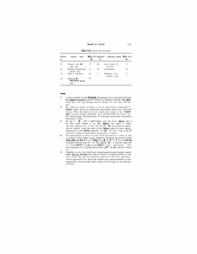
Table 15A.l Sector list (Contd)

2 4 9

Industry Industry name BEA I-O Industry Industry name BEA I-Ono. ?tO. no. NO.

3 3

3 4

3 5

Pr imary i ron & 3 7 6 9 A u t o r e p a i r & 7 . 5s t ee l mfg . s e r v i c e s

Primary nonferrous 3 8 7 0 Amusements 7 6meta l s mfg .

Me ta l con t a ine r s 3 9 7 1 Medleduc serv . 7 7

3 6nonprof . org.

Heating & 4 0fahrkted metalprod.

I wish to thank Gerard Dumenil, Dominique Levy and Alan Freemanfol MpfuI cummntnts, Edward Ochoa for making available hrs input-ou tpu t da t a , and Greg Bowgen and Ed Ch i l co te fo r t he i r he lp wi th th i sd a t a .My resu l t s a re s imi la r to Ochoa’s as fa r as in te r - indus t ry compar i sons oflabour values, prices of production and market prices are concerned(Ochoa , 1984) . But whereas he uses ac tua l g ross ou tpu t as the numer-aire, I use the s t andard commodi ty . Also , l ike B ienenfe ld my focus i s onthe determinants and behaviour of individual pricevalue deviations(Bienenfe ld , 1988) .The term (v . [K + AT]’ + ~sTl)/(a)~ is the ratio of the labour value ofthe direct capital advanced to the direct labour time required in produc-t i o n ( s e e e q u a t i o n 1 5 . 1 ) . I f o n e c a l l s t h i s t h e ith ‘ m a t e r i a l i z e d c o m p o s i -tion of capital’, then the ratio of the labour value of total capitaladvanced to total labour required = v. (H + Tf /vi) = l/q, is the irhv e r t i c a l l y i n t e g r a t e d m a t e r i a l i z e d c o m p o s i t i o n o f c a p i t a l .The approx ima t ion i s l i nea r i n w and r, bu t non - l i nea r i n r a lone as longas turnover times differ across industries. Suppose all turnover timeswerealike,sothatT=t0Z.ThenTr=B~T~B-’=T=t~I,andthestandard turnover time ts = (v . T, . Xs)/(v. Xs) = t, and the wage ratew = (1 - r/R)/(l + r. ts) = (1 - r/R)/(l + r. t). Subs t i tu t ing theseinto equation 15.11 yields p’(r) = ([I - r/R] + r e H)v, which is linearin r.Needless to say, we could have instead approximated output-capitalratios dilatly, dIlJ then used this to derive an approximation to thep r i c e s y s t e m . B u t t h e n t h e a n a l y t i c a l s i m p l i c i t y o f t h e p r i c e a p p r o x i m a -tion is generally lost. Since the simple price approximation is alsoempirically very powerful, there seems to be no gain in an alternateprocedu re .

The Labour Theory of Value2 5 0

6.

7.

8 .

9.

1 0 .

Bienenfeld (1988) chose to extend my (previously developed) linearapproximation by creating a quadratic approximation that is exact atboth r = 0 and r = R. But the economic interpretation of the termsinvo lved i s obscure .We do no t d i s t inguish be tween produc t ion and non-produc t ion labourin these particular estimates, but then it is not clear that such a distinc-Gun is appropriate wnen modellmg mdividual prices, since the cost ofactivities such as wholesale retail trade will show up in the total costs ofa commodi ty (Sha ikh and Tonak , 1994 , pp . 45-51) .The maximum profit rate R is the output-capital ratio of the standardsystem P&/P&, where both Xs and K&r a r e eva lua t ed i n any commonpr i ce sys t em (p r i ces o f p roduc t ion , marke t p r i ces o r labour va lues ) . Toa d j u s t f o r c a p a c i t y u t i l i z a t i o n , w e c a n e i t h e r c o m p a r e a c t u a l o u t p u t f l o wXs to utilized K ’ u, or normal capacity output XJu to actual capitalstock K. In either case the normal capacity maximum rate of profitR, = R/u.In recent private correspondence, Gerard Dumenil and DonminiqueT.&y hnvr chhown that this could be a sufficient oondition for nearlinearity. I had come to the same conclusion on the basis of my iterativeprocedure for linking Marx’s ‘transformed values’ to full prices ofproduction, since the speed of convergence depends on this ratio(Sha ikh , 1977 , ma thema t i ca l append ix , unpub l i shed ) .The Marxian standard commodity can be shown to be related to thevon Neumann ray (Sha ikh , 1984 , pp . 6&l).

References

Bienenfeld, M. (1988) ‘Regularities in Price Changes as an Effect ofChanges in Dis t r ibu t ion’ , Cambridge Journal of Economics , vo l . 12, no . 2 ,pp. 247-55.

Marzi, G. and Varri, P. (1977). Variazioni de Produttiva NeN’EconomiaItal iana: 1959-1967 (Bologna : Societa Edifrice 11 Mulino).

Marx, K. (1972) ‘Wage, Labour and Capital’, in R.C. Tucker (ed.), TheMarx-Engels Reader (New York: Norton).

Ochoa , E . (1984) ‘Labor Values and Pr ices of Product ion : An In te r indus t ryStudy of the U.S. Economy, 1947-1972’, unnublished PhD dissertation,New School for Social Research, New York.

Parys, W. (1982) ‘The Deviation of Prices from Labor Values’, AmericanEconomic Rev iew , vo l . 72 , no . 5 , pp . 1208-12 .

Pasinetti, L. L. (1977) Lectures on the Theory of Production (New York:Columbia Univers i ty Press) .

P a s i n e t t i , L . L . ( 1 9 8 1 ) Structural Change and Economic Growth (Cambr idge :Cambridge Univers i ty Press) .

Petrovir, P (1987) ‘The Deviation of Production Pricks from Laboul Values.Some Methodo logy and Empi r i ca l Ev idence ’ , Cambridge Journal o f Eco-nomics , vo l . 11 , no . 3 , pp . 197-210 .

Sche fo ld , B . ( 1976 ) ‘Re l a t i ve P r i ce s a s a Func t i on o f t he Ra t e o f P ro f i t : AM a t h e m a t i c a l N o t e ’ , Ze i t s chr i f t fur Nat ionalokonomie , vol . 36 , pp . 21-48 .

Anwnr M Shaikh 2 5 1

Schne ide r , H . (1964) Recen t Advances in Matr ix Theory (Madison: Univers i tyof Wisconsin Press) .

Shaikh, A. (1977) ‘Marx’s Theory of Value and the “TransformationProblem”‘, in J. Schwartz, The Subtle Anatomy of Capitalism (SantaMonica, CA: Goodyear) .

Shaikh, A. (1984) ‘The Transformation from Marx to Sraffa: Prelude to aCr i t i que o f t he Neo-Rica rd i ans ’ , i n E . Mande l and A. Freeman teds), Marx,R icardo , Sra f fa (London: Verso) .

Sha ikh , A . (1987) ‘The Fa l l ing Ra te o f P ro f i t and the Economic Cr i s i s in theU.S . ‘ , i n R . Cher ry e t a l . ( eds ) , The Emper i led Economy, book I (New York:U R P E ) .

Sha ikh , A . and E . A . Tonak (1994) Measur ing the Weal th o f Nations: ThePo l i t i ca l Economy o f Na t iona l Accoun t s (New York: Cambridge Univers i tyPress).

S ra f f a , P . (1963) Product ion o f Commodit ies by Means of Commodit ies ( C a m -br idge: Cambridge Univers i ty Press) .

15 the empirical strength of the labour theory of value frances/labthvalue.pdf · 15 the empirical...

Documents