Victor Chernozhukov and Ivan Fernandez-Val. 14.382 Econometrics. Spring 2017. Massachusetts Instituteof Technology: MIT OpenCourseWare, https://ocw.mit.edu. License: Creative Commons BY-NC-SA.

14.382 L8. LINEAR PANEL DATA MODELS UNDER STRICT AND WEAK EXOGENEITY

VICTOR CHERNOZHUKOV AND IV ´ ANDEZ-VAL AN FERN ´

Abstract. We discuss basic examples of linear panel data models and their estimation via the “fixed effects”, differencing, and correlated random effects approaches.

1. A Structural Linear Panel Model

1.1. The Setting. Here we consider the linear structural equations model (SEM) Yit itα + W f

itγ + Eit, (1.1)= ai + Dfitβ + Eit =: ai + X f Eit ⊥ (Xit, ai),

where i = 1, ..., n and t = 1, ..., T .

Here Yit is the outcome for an observational unit i at “time” t, Dit is a vector of variables of interest or treatments, whose predictive effect α we would like to estimate, Wit is a vector of covariates or controls including a constant, Xit simply stacks together Dit and Wit, and Eit is an error term normalized to have zero mean for each unit.

We shall assume that the vectors

Zi := {(Yit, X fit)

f}Tt=1,

that collect all the variables for the observational unit i, are i.i.d. across i. We note that this assumption does allow for arbitrary dependence of data for unit i across t, subject to other conditions specified below. In our analysis the temporal dimension T will be small and the cross-sectional dimension n will be large. Accordingly, we shall derive formal asymptotic results under the “large n, fixed T ” asymptotics, were n → ∞ and T is fixed. This type of scenario is often called the “short panel”.

The orthogonality condition stated will be strengthened below to various assumptions, which permit application of common estimation methods for performing inference on the target parameter α.

The random variable ai is the unobserved individual effect. It can be correlated to Xit, and so we can not omit it without introducing omitted variable bias that leads to

1

´ ´2 VICTOR CHERNOZHUKOV AND IVAN FERNANDEZ-VAL

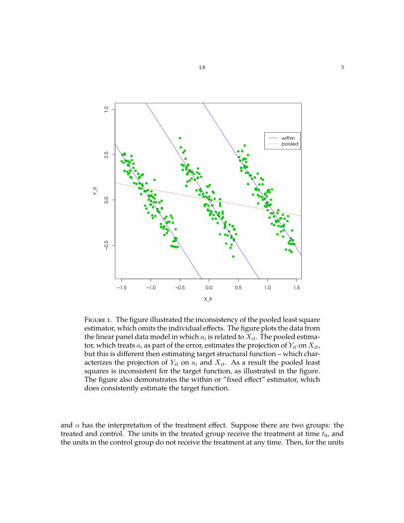
inconsistent estimates of the parameter of interest α. We can give context to this point by thinking of the case where ai is the unobserved individual’s innate ability, Yit is wage, Dit is education, and Wit are other characteristics of a person i at time t. Clearly omission of ai from the model would lead to an omitted variable bias and inconsistent estimation of the target parameter α for the usual reasons that we discussed in L2. Figure 1 illustrates the omitted variable bias problem in the linear panel model.

An important point to make here is the following.

Suppose Dit is randomly assigned conditional on ai and Wit, then α estimates a causal parameter – the average treatment effect. This is merely one of many suffi­cient conditions for causal interpretability of α. An example of another condition is the assumption of parallel trends underlying the difference-in-difference approach, as described below.

The individual effect ai is not observed and can not be identified or consistently es­timated from short panels. This fact is sometimes referred to as the incidental parameter problem, a term that was coined by Neyman and Scott [4]. However, the fact that we have panel data allows for the remarkable possibility to accommodate unobserved individual effects ai in the analysis explicitly. In fact, below we design identification and estimation strategies for the target parameter α that bypass the identification and consistent estimation of ai.

Before we continue, it is worth pointing out that Wit could contain a T -dimensional vector of indicators for time periods as a subvector, namely the vector

Qt = (0, 0, ..., 1, ..., 0)f

with 1 in the t-th position. In this case the model is said to include time effects.

1.2. The Difference-in-Difference Method. A very important special case of the problem that we consider is the “difference-in-difference” approach to identification. Here

Yit = ai + αDit + Witf β + Eit, (1.2)

where

• Dit is the indicator of unit i receiving the treatment at time t; • Wit are various other controls, for example, time dummies in the simplest case;

L8 3

−1.5 −1.0 −0.5 0.0 0.5 1.0 1.5

−0.5

0.0

0.5

1.0

X_it

Y_it

within

pooled

Figure 1. The figure illustrated the inconsistency of the pooled least square estimator, which omits the individual effects. The figure plots the data from the linear panel data model in which ai is related to Xit. The pooled estima­tor, which treats ai as part of the error, estimates the projection of Yit on Xit, but this is different then estimating target structural function – which char­acterizes the projection of Yit on ai and Xit. As a result the pooled least squares is inconsistent for the target function, as illustrated in the figure. The figure also demonstrates the within or ”fixed effect” estimator, which does consistently estimate the target function.

and α has the interpretation of the treatment effect. Suppose there are two groups: the treated and control. The units in the treated group receive the treatment at time t0, and the units in the control group do not receive the treatment at any time. Then, for the units

´ ´4 VICTOR CHERNOZHUKOV AND IVAN FERNANDEZ-VAL

in the treated group fE[Yis | Treated] = E[ai + Wisβ + Eis | Treated], s < t0,

E[Yit | Treated] = α + E[ai + Witf β + Eit | Treated], t ≥ t0.

It is tempting to take the difference:

E[Yit | Treated] − E[Yis | Treated] = α + E[(Wit − Wis)fβ + Eit − Eis | Treated], Change(s,t)

in an effort to identify the treatment effect α, but the trend term Change(s, t) does not necessarily vanish.

For the units in the control group: fE[Yis | Control] = E[ai + Wisβ + Eis | Control], s < t0,

E[Yit | Control] = E[ai + Witf β + Eit | Control], t ≥ t0.

If we take the difference, fE[Yit | Control] − E[Yis | Control] = E[(Wit − Wis) β + Eit − Eis | Control] . Change'(s,t)

Under the assumption of the parallel trends:

Change(s, t) = Changef(s, t),

which says that treatment and control groups experienced parallel trends apart from the treatment effect, we can take difference-of-the-difference to identify the treatment effect:

E[Yit − Yis | Treated] − E[Yit − Yis | Control] = α.

Thus under the assumption of parallel trends, we can identify the treatment effect α.

The structural linear panel data formulation allows us to incorporate the difference-in­difference approach as a special case. Under the assumption of parallel trends and other conditions specified below, we shall be able to identify and estimate α. Note that the as­sumption of parallel trends is more plausible when the treatment Dit is randomly assigned, but it also allows for non-random assignment even conditional on covariates.1 For exam­ple, if Yit is income and Dit is participation in a training program, it may be that Dit = 1 is assigned to those who had low income Yst in the pre-treatment period s < t0. In this case, we are still able to identify α under the assumption of the parallel trends for high and low-income groups in the absence of treatment. The plausibility of the assumption really depends on the context. It could be tested by seeing if group-specific trends enter the panel regression model as statistically insignificant.

1Of course, this is not the first time this happens in this course. Recall Wright’s instrumental variables model.

L8 5

2. Basic Identification and Estimation Strategies Under Strict Exogeneity

There are four methods for identification and estimation that we shall explore, which vary in terms of strength of assumptions needed for identification of α:

1. within-estimation or fixed effect estimation, 2. first-differencing, 3. correlated random effects, 4. pooled estimation or random effects.

The names listed above are conventional names given to the procedures, though some names are potentially misleading, as is usually the case.

2.1. Key approach I: within-groups or fixed effects approach. This approach eliminates the individual effects ai by individual demeaning. Define the operator D acting on doubly indexed random variables Vit as:

TT1 DVit = Vit − Vit.

T t=1

Apply this operator to the linear SEM (1.1) to obtain:

DYit = (DXit)fγ +DEit.

This has eliminated the individual effects. It is now very tempting to identify the param­eter γ as a projection coefficient and estimate it by least squares, but our assumptions are not sufficient for this purpose. In order to proceed in this way we need to have the orthog­onality condition:

T1 T

E[DXitDEit] = 0. (2.1)T

t=1

This condition states that the demeaned error terms are uncorrelated with the demeaned covariates, after averaging over t. With this assumption γ is equal to the projection co­efficient of DYit on DXit, where we aggregate across t = 1, . . . , T . The condition (2.1) is implied by the so-called strict exogeneity condition:

TEit ⊥ (X , a i), Xi := (Xis) (2.2)i s=1,

which states that the structural errors Eit are orthogonal to all lags and leads of Xit con­ditional on ai. This is potentially a restrictive condition, and does not hold with lagged dependent variables appearing as Xit. Note that it is hard to think of situations where (2.2) does not hold but (2.1) does for the causal parameter γ, so effectively we are impos­ing (2.2) when interpreting results as having causal meaning.

´ ´6 VICTOR CHERNOZHUKOV AND IVAN FERNANDEZ-VAL

The least squares estimation using the demeaned equation is called within-groups or fixed effects estimator. It can be seen as an exactly identified GMM estimator with the score function

TTg(Zi, γ) =

1 (DYit − DXit

f γ)DXit. (2.3)T

t=1

Because of the exact identification a simplified variance formula applies. It turns out that this approach is numerically equivalent to the the so-called least squares dummy variable (LSDV) estimator that applies OLS to the model:

= Qf iπ + DfYit itα + Wit

f β + uit,

where Qi is a n-dimensional vector of indicators for observational units with a 1 in the i-th position and 0’s otherwise, namely Qi = (0, 0, . . . , 1, . . . , 0). The elements of this vector are called fixed effects.

Note that here the GMM formulation takes care of the clustering problem – temporal dependence of data on observational unit i across time – by aggregating the data on unit i into one score. We can also use the panel bootstrap – which would be to simply bootstrap the independent observational units i or the scores in (2.3).

The strict exogeneity condition (2.2) contains “over identifying” restrictions, and we can set up a GMM estimator with the score function:

g(Zi, γ) = {(DYit − DXitf γ)Xi}Tt=1, Xi = (Xit)

Tt=1. (2.4)

Using this formulation we can obtain an efficient estimator for the causal parameter γ. Moreover, we can use the J-test to check the statistical validity of (2.2). Typically the ap­proach outlined in this paragraph is ignored in empirical work, but this is not a good practice. Note that here too we are taking care of the clustering problem by aggregating the data on unit i into one score.

We can construct an alternative GMM estimator based on a subset of linear combina­tions of the moment conditions implied by strict exogeneity using the score function:

g(Zi, γ) = {(DYit − DXitf γ)DXit}T (2.5)t=1.

This estimator might have better finite sample properties than the estimator based on (2.4) as it is based on a smaller number of informative moment conditions, T × dim Xit instead of T 2 × dim Xit. The J-test in this case can be interpreted as a test of time homogeneity of the parameter γ in the FE approach.

2.2. Key approach II: first differencing. This approach eliminates the individual effects ai by taking differences across time. Specifically, define the differencing operator Δ acting

L8 7

on doubly indexed random variables Vit by creating the difference ΔVit = Vit − Vit−1. Apply this operator to both sides of (1.1) to obtain:

ΔYit = ΔXitf γ +ΔEit, (2.6)

since Δai = 0. Thus differencing eliminates the individual effect. It is tempting to apply least squares to this equation to estimate γ, but the assumptions made so far do not guarantee that

TT1 EΔEitΔXit = 0, (2.7)

T − 1 t=2

which is necessary for γ to be a projection coefficient. So the researchers impose this con­dition implicitly when performing the first different estimation. This condition states that the innovation in the error terms is uncorrelated with the innovation in the covariates, af­ter averaging over t. With this assumption γ is equal to the projection coefficient of ΔYit on ΔXit, where we aggregate across t = 2, . . . , T . The assumption (2.7) is implied the strict exogeneity assumption (2.2) and it is hard to think of situations where strict exogeneity does not hold but (2.7) does for the causal parameter γ.

The assumption can serve as a basis of completely standard least squares estimation method with the i.i.d. data {Zi}n . We can formulate that as an exactly identified GMM

it

i=1problem with the score function:

g(Zi, γ) = 1 TT

(Δyit − ΔX f γ)ΔXit, (2.8)T − 1

t=2

so that GMM theory applies here, since {Zi}n are i.i.d. i=1

Note that the GMM formulation automatically takes care of the clustering problem – namely the fact that data for unit i could be dependent across t– by simply aggregating the scores within the cluster i. Note that we also can apply bootstrap for inference by simply bootstrapping observation units, or, equivalently bootstrapping the scores in (2.8).

Note however that the strict exogeneity (2.2) contains a lot of over-identifying informa­tion and could serve as a basis for a GMM method with the score function

g(Zi, γ) = {(Δyit − ΔXitf γ)Xi}Tt=2. (2.9)

This estimator will be more efficient than the previous one, and we can also use the J-statistic to test the validity of (2.7) (as well as validity of (2.2)). Ordinarily J-testing is not done in empirical work (which is bad practice), and one wonders if the results of many well-known studies will pass such a test. Again, the GMM theory applies here. Note that this formulation also automatically takes care of the clustering problem.

´ ´8 VICTOR CHERNOZHUKOV AND IVAN FERNANDEZ-VAL

As in the FE approach, we can construct an alternative GMM estimator based on a subset of linear combinations of the moment conditions implied by strict exogeneity using the score function:

g(Zi, γ) = {(ΔYit − ΔXitf γ)ΔXit}tT

=2. (2.10) This estimator might have better finite sample properties than the estimator based on (2.9) as it is based on a smaller number of informative moment conditions, (T − 1) × dim Xit instead of (T − 1)T × dim Xit. The J-test in this case can be interpreted as a test of time homogeneity of all the model parameters in the FD approach.

2.3. Other Approaches: Correlated Random Effects. In this approach, instead of trying to eliminate the individual effect ai, we model its dependence on the covariates:

TT1¯ ai = X ifλ + vi, vi ⊥ Xi, X

i = Xit. T

t=1

Then = X

ifλ + X fYit itγ + uit, uit = vi + Eit.

Under the strict exogeneity assumption (2.2), the parameters γ and λ can be identified as projection coefficients, and we can estimate the model by least squares. This corresponds to the GMM approach with the score function:

TTg(Zi, λ, γ) =

1 (Yit − Xi

fλ − Xitf γ)Xit, Xit = (X

i, Xit). T

t=1

It turns out that this approach is numerically equivalent to the within-groups estimator in the linear model. Still it is conceptually useful to have this approach discussed here.

As in the previous cases, there is a lot of over-identifying information and we can use the score function:

¯ g(Zi, λ, γ) = {(Yit − Xifλ − Xit

f γ)Xi}Tt=1

to set up the efficient GMM estimator and use the J-test to examine the validity of the model.

2.4. Other Approaches: Pooled or Random Effects Approach. This approach is by far the most restrictive. You still need to know about it, since people use this terminology quite often and you need to understand what they mean by it. In this approach we simply think that ai is uncorrelated with Xit and treat it as a part of the error term:

= X fYit itγ + vit, vit ⊥ Xit, vit = ai + Eit.

This means we can identify α as a projection coefficient and estimate it by least squares of Yit on Xit. The error terms vit are correlated across t, which is a form of “clustering”. We

L8 9

can easily take care of this dependence by using the score function:

TTg(Zi, γ) =

1 (Yit − Xit

f γ)Xit. (2.11)T

t=1

2.5. Which approach to use? The pooled estimator is the worst in terms of strength of assumptions. The minimal assumption (2.1) of the fixed effects approach and is neither stronger nor weaker than the minimal assumption (2.7) of the first differencing approach. It is always a good idea to test the underlying assumptions.

None of the assumptions made are suitable to the case where the strict exogeneity does not hold. Strict exogeneity requires the leads and lags of Xit to be uncorrelated with Eit. This assumption is violated for example when Xit contains lagged dependent variables. The first difference approach makes the slightly milder assumption of un­correlated differences, but it is still unsuitable, for example, when lags of Yit appear as Xit.

Example 1 (Lagged Dependent Variable). The last point requires elaboration. If the model is

Yit = ai + β Yi(t−1) +Eit, Xit

where Eit has zero mean conditional on ai and is independent across t. Then, strict exo­geneity clearly fails because Eit is not orthogonal to Xi(t+1) = Yit conditional on ai:

2E[YitEit | ai] = E[Eit | ai] = 0 .

Also the uncorrelated differences assumption fails because ΔEit is not orthogonal to ΔXit:

EΔXitΔEit = E(Yi(t−1) − Yi(t−2))(Eit − Ei(t−1)) = −EE2 = 0.i(t−1)

3. Getting More Sophisticated: Identification and Estimation under Weak Exogeneity

Once you understand how things work for the key approaches and how they easily fit in the GMM framework, you can easily modify them to best suit your empirical situations. Here is one example of how to do this, and it comes as a pleasant bonus for mastering the preceding section as well as the GMM material. In this example, we will focus on the differencing approach, but we could also consider de-meaning where one uses future values of the dependent variable to de-mean it and uses the past values of the regressors to demean them.

´ ´10 VICTOR CHERNOZHUKOV AND IVAN FERNANDEZ-VAL

3.1. A Model with Pre-Determined Regressors. Consider the linear SEM (1.1) with pre­determined regressors, namely

Eit ⊥ (Xit , ai), Xt := (Xit, Xi(t−1), . . . , Xi1).i

This is a weak exogeneity assumption. Note that this formulation can accommodate lagged dependent variables as part of Xit if Eit is not serially correlated.

We can adapt the first differences approach to this situation. Note that

ΔEit ⊥ Xt−1 .i

This means we can identify γ from the moment equations:

E(ΔYit − ΔXitf γ)Xi

t−1 = 0, t = 2, . . . , T. (3.1) The estimation and inference can be done using GMM with the score function

g(Zi, γ) = {(ΔYit − ΔXitf γ)Xi

t−1}Tt=2. (3.2) This estimation method subsumes as a special case the Arellano-Bond [3]’s estimation ap­proach for models with a lagged dependent variable.

As in the strictly exogenous case, we can construct an alternative GMM estimator based on a subset of linear combinations of the moment conditions implied by weak exogeneity using the score function:

g(Zi, γ) = {(ΔYit − ΔXitf γ)Xi(t−1)}Tt=2. (3.3)

This estimator might have better finite sample properties than the estimator based on (3.2) as it is based on a smaller number of informative moment conditions. The J-test in this case can be interpreted as a test of time homogeneity of all the model parameters. We can further reduce the number conditions by averaging over t resulting on the score function

TT1 g(Zi, γ) = (ΔYit − ΔXit

f γ)Xi(t−1),T − 1 t=2

which just-identities the parameter γ. This method subsumes as a special case the Anderson-Hsiao [2] estimator for models with a lagged dependent variable.

3.2. A Model with Pre-Determined Instruments. As a further generalization we consider the linear structural equations model (SEM)

Yit = ai + Ditf α + Wit

f β + Eit =: ai + Xitf γ + Eit,

where i = 1, ..., n and t = 1, ..., T , and where we have pre-determined instruments:

Eit ⊥ (Mit , ai), M t := (Mit,Mi(t−1), ...). (3.4)i

where Mit are technical instruments that contain Wit, but don’t contain Dit. For example, we can think about modeling aggregate demand equations across different markets i and

L8 11

across different time periods, where Dit is the price. The instruments Mit could consist of various supply shifters as well as controls Wit.

Then (3.4) implies ΔEit ⊥ M t−1 . (3.5)i

This means we can identify γ from the moment equations:

E(ΔYit − ΔXitf γ)Mi

t−1 = 0. (3.6) The estimation and inference can be done using GMM with the score function

g(Zi, γ) = {(ΔYit − ΔXitf γ)Mi

t−1}Tt=2. (3.7)

As before the GMM formulation takes care of clustering by simply defining the scores appropriately.

4. The Effects of Expending on Academic Performance

We illustrate the methods of Section 2 with an empirical application on the effect of school resources per student on test pass rates following Papke (2005) [5]. We use data from annual Michigan School Reports (MSR) on 550 elementary schools in Michigan for the period from 1992 through 1998. This period covers 1994, when Michigan carried out a school finance reform to equalize spending across K-12 schools. The purpose of this re­form is to offer equal educational opportunities and to improve student performance. The outcome variable Yit is the percent of students passing a fourth-grade math test from the Michigan Educational Assessment Program in school i at year t. The explanatory variables Xit include the logarithm of per student spending, logarithm of per student spending in the previous year, the fraction of the students receiving free lunch, and the logarithm of school enrollment. Table 1 gives descriptive statistics for the variables used in the analysis.

Table 1. Descriptive Statistics

Mean SD Math Pass Rate 55.43 18.20 Expenditure 5,496 1,151 Lunch 27.20 15.41 Enrollment 3,044 8,153

We estimate the model (1.1) using several approaches:

(1) Pooled: pooled approach that assumes that Xit is orthogonal to the school unob­served effect ai.

(2) FD: first differencing approach based on the moment conditions (2.7).

´ ´12 VICTOR CHERNOZHUKOV AND IVAN FERNANDEZ-VAL

(3) GMM-FD1: first differencing approach based on two-step GMM with the score function (2.10). The first-step uses the FD estimator to construct the optimal weight­ing matrix.

(4) GMM-FD2: first differencing approach based on two-step GMM with the score function (2.9), which exploits all the restrictions implied by strict exogeneity. The first-step uses the FD estimator to construct the optimal weighting matrix.

(5) FE: fixed effects approach based on the moment conditions (2.1). (6) GMM-FE1: fixed effects approach based on two-step GMM with score function

(2.5). The first-step uses the FE estimator to construct the optimal weighting matrix. (7) GMM-FE2: fixed effects approach based on two-step GMM with score function

(2.4), which exploits all the restrictions implied by strict exogeneity. The first-step uses the FE estimator to construct the optimal weighting matrix.

For each approach we compute estimates, analytical standard errors clustered at the school level, and bootstrap standard errors based on resampling schools with replacement. We also report the results of the J-test for the overidentifying restrictions of the GMM-FD1, GMM-FD2, GMM-FE1 and GMM-FE2 approaches.

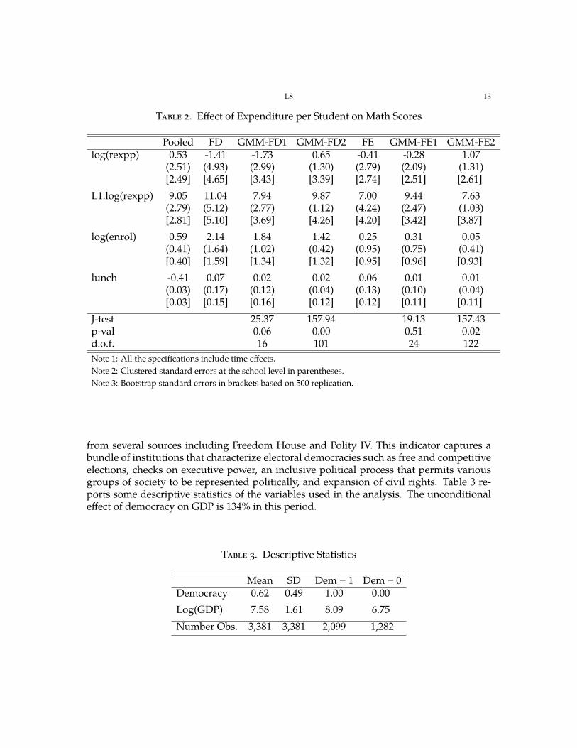
Table 2 presents the results. All the approaches yield positive and significant effects of increasing expenditure per student the previous year on current math score passing rates. The delay on the effect is due to the timing of the tests and spending variables: the test are administered early in the second semester, whereas the spending is the allocation for the entire school year. According to the analytical standard errors, using all the strict exogeneity restrictions substantially increases the precision of the estimates. However, we should be cautious with this result as analytical standard errors might provide a poor approximation to the variability of two-step GMM estimators in the presence of many (potentially weak) moment conditions.2 Bootstrap provides standard errors that are more stable across the different approaches. Time homogeneity of all the model parameters cannot be rejected at the 5% level, although only marginally for the GMM-FD1. The strict exogeneity overidentifying restrictions are rejected at the 5% level with both GMM-FD2 and GMM-FE2.

5. Causal Effect of Democracy on Economic Growth

We illustrate the methods of Section 3 with an application to the causal effect of democ­racy on economic growth based on Acemoglu, Naidu, Restrepo and Robinson (2014) [1]. We use a balanced panel of 147 countries over the period from 1987 through 2009 extracted from the data set used in [1]. The outcome variable Yit is the logarithm of GDP per capita in 2000 USD as measured by the World Bank for country i at year t. The treatment variable of interest Dit is a democracy indicator constructed in [1], which combines information

2[6] derived a correction for analytical standard errors of two-step GMM estimators.

L8 13

Table 2. Effect of Expenditure per Student on Math Scores

Pooled FD GMM-FD1 GMM-FD2 FE GMM-FE1 GMM-FE2 log(rexpp) 0.53

(2.51) [2.49]

-1.41 (4.93) [4.65]

-1.73 (2.99) [3.43]

0.65 (1.30) [3.39]

-0.41 (2.79) [2.74]

-0.28 (2.09) [2.51]

1.07 (1.31) [2.61]

L1.log(rexpp) 9.05 (2.79) [2.81]

11.04 (5.12) [5.10]

7.94 (2.77) [3.69]

9.87 (1.12) [4.26]

7.00 (4.24) [4.20]

9.44 (2.47) [3.42]

7.63 (1.03) [3.87]

log(enrol) 0.59 (0.41) [0.40]

2.14 (1.64) [1.59]

1.84 (1.02) [1.34]

1.42 (0.42) [1.32]

0.25 (0.95) [0.95]

0.31 (0.75) [0.96]

0.05 (0.41) [0.93]

lunch -0.41 0.07 0.02 0.02 0.06 0.01 0.01 (0.03) [0.03]

(0.17) [0.15]

(0.12) [0.16]

(0.04) [0.12]

(0.13) [0.12]

(0.10) [0.11]

(0.04) [0.11]

J-test 25.37 157.94 19.13 157.43 p-val d.o.f.

0.06 16

0.00 101

0.51 24

0.02 122

Note 1: All the specifications include time effects. Note 2: Clustered standard errors at the school level in parentheses. Note 3: Bootstrap standard errors in brackets based on 500 replication.

from several sources including Freedom House and Polity IV. This indicator captures a bundle of institutions that characterize electoral democracies such as free and competitive elections, checks on executive power, an inclusive political process that permits various groups of society to be represented politically, and expansion of civil rights. Table 3 re­ports some descriptive statistics of the variables used in the analysis. The unconditional effect of democracy on GDP is 134% in this period.

Table 3. Descriptive Statistics

Mean SD Dem = 1 Dem = 0 Democracy 0.62 0.49 1.00 0.00 Log(GDP) 7.58 1.61 8.09 6.75 Number Obs. 3,381 3,381 2,099 1,282

´ ´14 VICTOR CHERNOZHUKOV AND IVAN FERNANDEZ-VAL

We control for unobserved country effects and rich dynamics of GDP using the linear panel model

pTYit = ai + αDit + βj Yi(t−j) + Eit, i = 1, . . . , n, t = p + 1, . . . , T,

j=1

where we assume that

Eit ⊥ (Xit , ai), Xi

t = (Dit, . . . , Di1, Yi(t−1), . . . , Yi1). (5.1)

This assumption implies that democracy and past GDP are orthogonal to contemporane­ous and future GDP shocks, and that the error Eit is serially uncorrelated once we include sufficiently many lags of GDP.3 Following the preferred specification in [1], we include four lags (p = 4).

Table 4. Effect of Democracy on Economic Growth

Predictive Causal Pooled FD FE GMM-FD1 GMM-FD2

Democracy (×100)

0.46 (0.26) [0.26]

0.94 (1.20) [1.20]

1.89 (0.65) [0.66]

4.45 (2.77) [2.75]

3.91 (1.70) [1.61]

L1.log(gdp) 1.33 (0.05) [0.05]

0.33 (0.05) [0.06]

1.15 (0.05) [0.05]

1.30 (0.14) [0.15]

1.00 (0.07) [0.07]

L2.log(gdp) -0.18 (0.06) [0.07]

0.17 (0.04) [0.04]

-0.12 (0.06) [0.06]

-0.15 (0.28) [0.22]

-0.08 (0.06) [0.07]

L3.log(gdp) -0.11 (0.05) [0.05]

0.06 (0.02) [0.02]

-0.07 (0.04) [0.04]

-0.43 (0.28) [0.23]

-0.04 (0.04) [0.04]

L4.log(gdp) -0.05 (0.03) [0.03]

-0.05 (0.04) [0.04]

-0.08 (0.02) [0.03]

0.18 (0.14) [0.13]

-0.08 (0.03) [0.03]

J-test 70.71 130.23 p-value d.o.f.

0.00 31

1.00 463

Note 1: All the specifications include time effects. Note 2: Clustered standard errors at the country level in parentheses. Note 3: Bootstrap standard errors in brackets based on 500 replications.

3All the variables are net of time effects.

L8 15

Table 4 presents the results. The estimates based on the weak exogeneity condition (5.1) are reported in the columns labelled as GMM-FD1 and GMM-FD2.4 GMM-FD1 applies two-step GMM with the score function (3.3) with

Xit = (Dit, Yi(t−1), . . . , Yi(t−4)), γ = (α, β1, . . . , β4), (5.2) which uses only a subset of the moment conditions in (5.1). GMM-FD2 applies two-step GMM with the score function (3.2), which uses all the moment conditions in (5.1), with the same Xit and γ as in (5.2) . In both cases we test the overidentifying restrictions us­ing the J-test. The rest of the columns report estimates of predictive effects based on the pooled, first differencing and fixed effects approaches of Section 2 with the score functions (2.11), (2.8) and (2.3), respectively. None of these approaches is consistent for the causal parameters identified by (5.1) under large n fixed T asymptotics.5 For each method, we re­port analytical standard errors clustered at the country level and bootstrap standard errors based on resampling countries without replacement. The GMM-FD2 approach finds that a transition to democracy increases economic growth by almost 4% in the first year, and about 20% in the long run.6 The J-test does not reject the weak exogeneity overidentifying restrictions in (5.1). The GMM-FD1 approach yields short run effects similar to FD-GMM2, but more than double run effects of 46.7% and clearly reject the overidentifying restrictions in (3.3). This does raise the concern about the statistical validity of the model and warrants further investigation. The discrepancy in the conclusion of the J-test might be due to lack of power in the GMM-FD2 due to simultaneous testing of many restrictions, most of them (possibly) weak moment conditions. As expected, the FE predictive estimates are closer to their causal counterparts than the pooled and FD estimates because T is large, T = 19 after using the first 4 periods as initial conditions.

Appendix A. Problems

(1) Implement standard panel data estimators (fixed effects, first differences, or Arellano-Bond approach) for the first or second empirical example. These are implemented in standard software such as Stata or R. Very briefly explain the assumptions you need to make for these estimators to be consistent for causal effects, and why these assumptions may or may not hold in these examples. Very briefly explain how you are taking care of clustering.

(2) (Optional Bonus Problem.) Implement the GMM-FE1 and GMM-FE2 estimators for the first empirical example and GMM-FD1 for the second empirical example. Report results of J-tests. Explain very briefly what you are doing. Extra ”plus” for

4We obtain the estimates with the command pgmm of the package plm in R. 5The fixed effects estimator is consistent under asymptotic sequences where n, T → ∞ because it has

asymptotic bias of order O(T −1). 6The long-run effect is calculated as α/(1− pj=1 βj ), and corresponds to the effect of a permanent transition

to democracy.

´ ´16 VICTOR CHERNOZHUKOV AND IVAN FERNANDEZ-VAL

finding problems with the posted R-code or the empirical results reported in the lecture note.

References

[1] Daron Acemoglu, Suresh Naidu, Pascual Restrepo, and James A. Robinson. Democ­racy Does Cause Growth. NBER Working Papers 20004, National Bureau of Economic Research, Inc, March 2014.

[2] T. W. Anderson and Cheng Hsiao. Formulation and estimation of dynamic models using panel data. J. Econometrics, 18(1):47–82, 1982.

[3] Manuel Arellano and Stephen Bond. Some tests of specification for panel data: Monte carlo evidence and an application to employment equations. The Review of Economic Studies, 58(2):277–297, 1991.

[4] J. Neyman and E. L. Scott. Consistent estimates based on partially consistent observa­tions. Econometrica, 16(1):1–32, 1948.

[5] Leslie E. Papke. The effects of spending on test pass rates: evidence from Michigan. Journal of Public Economics, 89(5-6):821–839, June 2005.

[6] Frank Windmeijer. A finite sample correction for the variance of linear efficient two-step gmm estimators. Journal of Econometrics, 126(1):25 – 51, 2005.

MIT OpenCourseWarehttps://ocw.mit.edu

14.382 EconometricsSpring 2017

For information about citing these materials or our Terms of Use, visit: https://ocw.mit.edu/terms.