14 three-dimensional radiative transfer in vegetation...

14 Three-Dimensional Radiative Transfer inVegetation Canopies

Yuri Knyazikhin, Alexander Marshak, and Ranga B. Myneni

14.1 Introduction

Interaction of photons with a host medium is described by a linear transport equa-tion. This equation has a very simple physical interpretation; it is a mathematicalstatement of the energy conservation law. In spite of the different physics behind ra-diation transfer in clouds and vegetation, these media have certain macro and micro-scale features in common. First, both are characterized by strong horizontal andvertical variations, and thus their three-dimensionality is important to correctly de-scribe the photon transport. Second, the radiation regime is substantially influencedby the sizes of scattering centers that constitute the medium. Drop and leaf size dis-tribution functions are the most important variables characterizing the micro-scalestructure of clouds and vegetation canopies, respectively. Third, the independent (orincoherent) scattering concept underlies the derivation of the extinction coefficientand scattering phase function in both theories (van de Hulst, 1980, p. 4-5); (Ross,1981, p. 144). This allows the transport equation to relate micro-scale properties ofthe medium to the photon distribution in the entire medium. From a mathematicalpoint of view, these three features determine common properties of radiative transferin clouds and vegetation.

However, the governing radiative transfer equation for leaf canopies, in boththree-dimensional (3D) and one-dimensional (1D) geometries, has certain uniquefeatures. The extinction coefficient is a function of the direction of photon travel.Also, the differential scattering cross-section is not, as a rule, rotationally invariant,i.e., it generally depends on the absolute directions of photon travel and′, andnot just the scattering anglearccos • ′. Finally, the single scattering albedo isalso a function of spatial and directional variables. These properties make solvingof the radiative transfer equation more complicated; for example, the expansion ofthe differential scattering cross-section in spherical harmonics (see, Chap. 4) cannotbe used.

In contrast to radiative transfer in clouds, the extinction coefficient in vegeta-tion canopies introduced by Ross (1981) is wavelength independent, considering thesize of scattering elements (leaves, branches, twigs, etc.) relative to the wavelengthof solar radiation. Although the scattering and absorption processes are differentat different wavelengths, the optical distance between two arbitrary points withinthe vegetation canopy does not depend on the wavelength. This spectral invariance

338 Knyazikhin et al.

results in various unique relationships which, to some degree, compensate for diffi-culties in solving the radiative transfer equation due to the above mentioned featuresof the extinction and the differential scattering cross-sections.

We idealize a vegetation canopy as a medium filled with small planar elementsof negligible thickness. We ignore all organs other than green leaves in this chapter.In addition, we neglect finite size of vegetation canopy elements. Thus, the vegeta-tion canopy is treated as a gas with nondimensional planar scattering centers, i.e., aturbid medium. In other words, one cuts leaves resided in an elementary volume into“dimensionless pieces” and uniformly distributes them within the elementary vol-ume. Two variables, the leaf area density distribution function and the leaf normaldistribution are used in the theory of radiative transfer in vegetation canopies to con-vey “information” about the total leaf area and leaf orientations in the elementaryvolume before “converting the leaves into the gas.”

Fig. 14.1.Mean reflectance of evegreen broadleaf forest at near-infrared (865nm) wavelengthas a function of phase angle (after (Breon et al., 2001)). Data were acquired by the POLDER(Polarization and Directionality of the Earth’s Reflectances) multi-angle spaceborne instru-ment (Deschamps et al., 1994). Phase angles are shown with a negative sign if the POLDERview azimuth was greater than 180◦. Canopy reflectances exhibit a sharp peak about theretro-illumination direction (the “hot spot ”effect) which classical transport equation can notpredict.

14 3D Radiative Transfer in Vegetation Canopies 339

It should be noted that the turbid medium assumption is violated in the caseof vegetation canopies and, therefore, finite size scatters can cast shadows. Thiscauses a very sharp peak in reflected radiation about the retro-solar direction. Thisphenomenon is referred to as the “hot spot ”effect (Fig. 14.1). It is clear that pointscatters cannot cast shadows and thus, the turbid medium concept in its originalformulation (Ross, 1981) fails to predict or duplicate experimental observation ofexiting radiation about the retro-illumination direction (Kuusk, 1985; Gerstl andSimmer, 1986; Marshak, 1989; Verstrate et al., 1990). Recently, Zhang et al. (2002)showed that if the solution to the radiative transfer equation is treated as a Schwartzdistribution, then an additional term must be added to the solution of the radiativetransfer equation. This term describes the hot spot effect. This result justifies theuse of the transport equation as the basis to model canopy-radiation regime. Herewe will follow classical radiative transfer theory in vegetation canopies proposed byRoss (1981) with emphasis on canopy spectral response to the incident radiation. Forthe mathematical theory of Schwartz distributions applicable to the transport equa-tion, the reader is referred to Germogenova (1986), Choulli and Stefanov (1996) andAntyufeev and Bondarenko (1996).

Finally, what are our motivations to include a chapter on radiative transfer invegetation canopies in the book on atmospheric radiative transfer? Why is the veg-etation canopy a special type of surface? First of all, vegetated surfaces play an im-portant role in the Earth’s energy balance and have a significant impact on the globalcarbon cycle. The problem of accurately evaluating the exchange of carbon betweenthe atmosphere and terrestrial vegetation has received scientific (IntergovernmentalPanel on Climate Change (IPCC), 1995) and, also, political attention (Steffen etal., 1998). The next motivation is both the similarity and the unique features of theradiative transfer equations that govern radiative transfer processes in these neigh-bouring media. Because of their radiative interactions, the vegetation canopy andthe atmosphere are coupled together; each serves as a boundary condition to theradiative transfer equations in the adjacent medium. To better understand radiativeprocesses in these media we need an accurate description of their interactions. Thischapter complements the rest of the book and mainly deals with radiative transferin vegetation canopies. The last section outlines a technique needed to describe thecanopy-clouds interaction.

14.2 Vegetation Canopy Structure and Optics

Solar radiation scattered from a vegetation canopy results from interaction of pho-tons traversing through the foliage medium, bounded at the bottom by a radiativelyparticipating surface. Therefore to estimate the canopy radiation regime, three im-portant features must be carefully formulated. They are (1) the architecture of indi-vidual plants and of the entire canopy; (2) optical properties of vegetation elements(leaves, stems) and soil; the former depends on physiological conditions (water sta-tus, pigment concentration); and (3) atmospheric conditions which determine the in-cident radiation field (Ross, 1981). For radiative transfer in clouds, they correspond


respectively to cloud micro (e.g., distribution of cloud drop sizes) and macro (e.g.,cloud type and geometry) structures, cloud drop optical properties, and boundary (il-lumination) conditions. Note that radiation incident on the top of the atmosphere isa monodirectional solar beam while the vegetation canopies are illuminated both bymonodirectional beam attenuated by the atmosphere and radiation scattered by theatmosphere (diffuse radiation). Photon transport theory aims at deriving the solar ra-diation regime, both within the vegetation canopy and cloudy atmosphere, using theabove mentioned attributes as input data. For vegetation canopy, the leaf area densitydistribution,uL, leaf normal orientation distribution, gL, leaf scattering phase func-tion, L, and boundary conditions specify these input (Ross, 1981; Myneni et al.,1990; Knyazikhin, 1991; Pinty and Verstraete, 1997). We will start with definitionsof these variables.

14.2.1 Vegetation Canopy Structure

At the very least, two important wavelength independent structural attributes - leafarea density and leaf normal orientation distribution functions - need to be definedin order to quantify vegetation-photon interactions.

The one-sided green leaf area per unit volume in the vegetation canopy at loca-tion x = (x, y, z) is defined as the leaf area density distributionuL(x) (in m2/m3 orsimply m−1). Realistic modeling ofuL(x) is a challenge for it requires simulatedvegetation canopies with computer graphics and tedious field measurements. Thedimensionless quantity

L(x, y) =

H∫

0

dzuL(x, y, z), (14.1)

is called theleaf area index, one-sided green leaf area per unit ground area at(x, y).HereH is depth of the vegetation canopy.

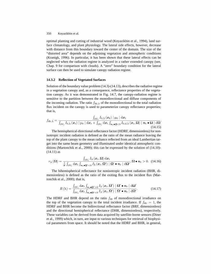
Figures 14.2 and 14.3 demonstrate a computer-generated Norway spruce standand corresponding leaf area indexL(x, y) at a spatial resolution of 50 cm (i.e., dis-tribution of the mean leaf area indexL(x, y) taken over each of 50 by 50 cm groundcells). Leaf area index is the key variable in most ecosystem productivity models,and in global models of climate, hydrology, biogeochemistry and ecology which at-tempt to describe the exchange of fluxes of energy, mass (e.g., water and CO2), andmomentum between the surface and the atmosphere. In order to quantitatively andaccurately model global dynamics of these processes, differentiate short-term fromlong-term trends as well as to distinguish regional from global phenomena, this pa-rameter must be collected often for a long period of time and should represent everyregion of the Earth land surface. The leaf area index has been operationally producedfrom data provided by two instruments, the moderate resolution imaging specrora-diometer (MODIS) and multiangle imaging spectroradiometer (MISR), during theEarth Observing System (EOS) Terra mission (Myneni et al., 2002). Global map ofMODIS leaf area index at 1 km resolution is shown in Fig. 14.4. Note that the the-ory of radiative transfer in vegetation canopies presented in this chapter underlies


Fig. 14.2.Photo shows a Norway spruce stand about 50 km of Goettingen in the Harz moun-tains. The forest is about 45 years old and situated on the south slope. For the sake of detailedexamination of the canopy structure, a site covering an area of approximately 40x40 m2 waschosen (shown as a square) and taken as representative for the whole stand. The canopyspace is limited by the slope and a plane parallel to the slope at the height of the tallest treeof 12.5 m. There are in total 297 trees in the sample stand. The tree trunk diameters variedfrom 6 to 28 cm. The stand is rather dense but with some localized gaps. For the needs ofmodeling the trees were divided into five groups with respect to the tree trunk diameter. Amodel of a Norway spruce based on fractal theory was then used to build a representative ofeach group (Kranigk and Gravenhorst, 1993; Kranigk et al., 1994; Knyazikhin et al., 1996).Given the distribution of tree trunks in the stand, the diameter of each tree, the entire samplesite was generated. Bottom panels demonstrate the computer generated Norway spruce standshown from different directions: crown map (left panel), front view (middle panel), and crosssection (right panel).

the retrieval technique for retrieving leaf area index from satellite data (Knyazikhin,1991; Knyazikhin and Marshak, 1991).

LetL be the upward normal to the leaf element. The following function char-acterizes the leaf normals distribution:(1/2�)gL(L) is the probability density ofthe leaf normals distribution with respect to the upward hemisphere(�+)

12�

∫

�+

dLgL (L) = 1. (14.2)


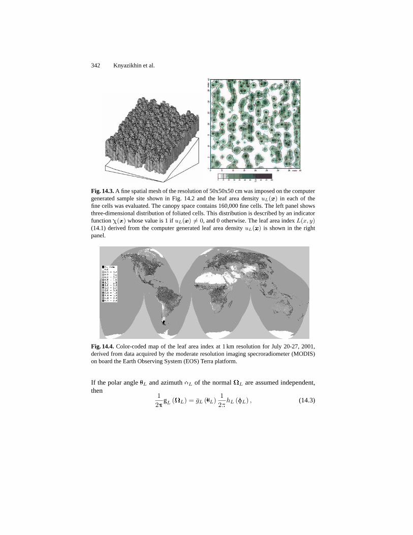
Fig. 14.3.A fine spatial mesh of the resolution of 50x50x50 cm was imposed on the computergenerated sample site shown in Fig. 14.2 and the leaf area densityuL(x) in each of thefine cells was evaluated. The canopy space contains 160,000 fine cells. The left panel showsthree-dimensional distribution of foliated cells. This distribution is described by an indicatorfunction�(x) whose value is 1 ifuL(x) 6= 0, and 0 otherwise. The leaf area indexL(x, y)(14.1) derived from the computer generated leaf area densityuL(x) is shown in the rightpanel.

Fig. 14.4.Color-coded map of the leaf area index at 1 km resolution for July 20-27, 2001,derived from data acquired by the moderate resolution imaging specroradiometer (MODIS)on board the Earth Observing System (EOS) Terra platform.

If the polar angle�L and azimuth�L of the normalL are assumed independent,then

12�

gL (L) = gL (�L)12�

hL (�L) , (14.3)


wheregL(�L) and(1/2�)hL(�L) are theprobability density functions of leaf nor-mal inclinationandazimuth, respectively, and

�/2∫

0

gL (�L) sin �Ld�L = 1,12�

2�∫

0

hL (�L) d�L = 1. (14.4)

The functions gL(L), gL(�L) andhL(�L) depend on the locationx in the vegeta-tion canopy but this is implicit in the remainder of the text.

The following example model distribution functions for leaf normal inclinationwere proposed by DeWit (1965):planophile- mostly horizontal leaves,erectophile-mostly erect leaves;plagiophile- mostly leaves at 45 degrees;extremophile- mostlyhorizontal and vertical leaves; anduniform - all possible inclinations. These distri-butions can be expressed as (cf. Bunnik, 1978),

Planophile: gL (�L) =2�

(1 + cos 2�L) , (14.5a)

Erectophile: gL (�L) =2�

(1− cos 2�L) , (14.5b)

Plagiophile: gL (�L) =2�

(1− cos 4�L) , (14.5c)

Extremophile: gL (�L) =2�

(1 + cos 4�L) , (14.5d)

Uniform: gL (�L) = 1. (14.5e)

Example distributions of the leaf normal inclination are shown in Fig. 14.5.Certain plants, such as soybeans and sunflowers, exhibit heliotropism, where the

leaf azimuths have a preferred orientation with respect to the solar azimuth. A simplemodel forhL in such canopies ishL(�L,�0) = 2 cos2(�0 − �L − �) where the pa-rameter� is the difference between the azimuth of the maximum of the distributionfunctionhL and the fixed azimuth of the incident photon�0 (cf. Verstraete, 1987).In the case of diaheliotropic distributions, which tend to maximize the projected leafarea to the incident stream� = 0. On the other hand, paraheliotropic distributionstends to minimize the leaf area projected to the incident stream,� = �/2. A moregeneral model for the leaf normal orientations is the�-distribution, the parameters ofwhich can be obtained from fits to field measurements of the leaf normal orientation(Goel and Strebel, 1984).

14.2.2 Vegetation Canopy Optics

A photon incident on a leaf surface can either be absorbed or scattered. If the scat-tered photon emerges from the same side of the leaf as the incident photon, the eventis termed reflection. Likewise, if the scattered photon exits the leaf from the oppositeside, the event is termed transmission. Scattering of solar radiation by green leavesdoes not involve frequency shifting interactions, but is dependent on the wavelength.


Fig. 14.5.The probability density functions for planophile (14.5a), erectrophile (14.5b), pla-giophile (14.5c), extremophile (14.5d) and uniform (14.5e) distributions.

The angular distribution of radiant energy scattered by a leaf element is a keyvariable, and is specified by the leaf element scattering phase function L,�(′ →,L). For a leaf with upward normalL, this phase function is the fraction ofintercepted energy, from photon initially traveling in′, that is scattered into anelement of solid angled about.

Radiant energy may be incident on the upper or the lower sides of the leaf el-ement and the scattering event may be either reflection or transmission. Integra-tion of the leaf scattering phase function over the appropriate solid angles gives thehemispherical leaf reflectance�L,�(′,L) and transmittance�L,�(′,L) coef-ficients. The leaf scattering phase function when integrated over all scattered photondirections(�) yields the leaf albedo,

!L,� (′,L) =∫

�

L,� (′ → ,L) d (14.6)

where� is the unit sphere. The leaf albedo!L,� (′,L) is simply the sum of�L,�(′,L) and�L,�(′,L). The reflectance and transmittance of an individualleaf depends on wavelength, tree species, growth conditions, leaf age and its locationin the canopy.


A photon incident on a leaf element can either be specularly reflected from thesurface depending on its roughness or emerge diffused from interactions in the leafinterior. Some leaves can be quite smooth from a coat of wax-like material, whileother leaves can have hairs making the surface rough. Light reflected from the leafsurface can be polarized as well. Photons that do not suffer leaf surface reflection en-ter the interior of the leaf, where they are either absorbed or refracted because of themany refractive index discontinuities between the cell walls and intervening air cav-ities. Photons that are not absorbed in the interior of the leaf emerge on both sides,generally diffused in all directions. Figure 14.6 shows typical diffuse hemisphericalreflectance,�L,�(−L,L), and transmittance,�L,�(−L,L), spectra of an in-dividual leaf under normal illumination. For more details on diffuse leaf scatteringand specular reflection from the leaf surface, the reader is referred to Walter-Sheaand Norman (1991), and Vanderbilt et al. (1991).

Fig. 14.6.Typical reflectance and transmittance spectra of an individual plant leaf from 400to 2000 nm for normal incidence.

14.2.3 Extinction, Scattering and Absorption Events

To derive an expression for the extinction coefficient consider photons atx travelingalong. The total extinction coefficient is the probability, per unit path length of


travel, that the photon encounters a leaf element,

� (x,) = uL (x) G (x,) , (14.7)

whereG(x,) is thegeometry factorfirst proposed by Ross (1981), defined as theprojection of unit leaf area atx onto a plane perpendicular to the direction of photontravel, i.e.,

G (x,) =12�

∫

�+

dLgL (x,L) | •L | . (14.8)

The geometry factorG satisfies(2�)−1∫�+

G(x,)d = 1/2. Upon collisionwith a leaf element, a photon can be either absorbed or scattered. So the extinctioncoefficient can be broken down into its scattering and absorption components,� =�s,� + �a,�. It is important to note that the geometry factor is an explicit functionof the direction of photon travel in the general case of non-uniformly distributedleaf normals. This imbues directional dependence to the extinction coefficients in thecase of vegetation canopies. Only in the case of uniformly distributed leaf normals(G = 1/2) its dependence on disapears. A noteworthy point is thewavelengthindependenceof �, that is, the extinction probabilities for photons in vegetationmedia are determined by the structure of the canopy rather than photon frequencyor the optics of the canopy.

Consider photons impinging on leaf elements of area densityuL at locationxalong′. The probability density, per unit path length, that these photons wouldbe intercepted and then scattered in to the direction is given by the differentialscattering coefficient

�′s,� (x,′ → ) = uL (x)1�� (x,′ → ) ,

= uL (x)12�

∫

�+

dLgL (x,L) | ′ •L | L,� (′ → ,L) ,

(14.9)

where(1/�)�λ is thearea scattering phase functionfirst proposed by Ross (1981).The scattering phase function combines diffuse scattering from the interior of a leafand specular reflection from the leaf surface. For more details on the diffuse andspecular components of the area scattering phase function, the reader is referred toRoss (1981), Marshak (1989), Myneni (1991), Knyazikhin and Marshak (1991).

It is important to note that the differential scattering coefficient is an explicitfunction of the polar coordinates of′ and, that is, non-rotationally invariant.Only in some limited cases it can be reduced to the rotationally invariant form,�′s,�(x, → ′) ≡ �′s,�(x, •′). This property precludes the use of Legendrepolynomial expansions and of the addition theorem often used in transport theoryfor handling the scattering integral (see, Chap. 4).


Integration of the differential scattering coefficient (14.9) over all scattered pho-ton directions results in the scattering coefficient,

�s,� (x,) = uL (x)12�

∫

�+

dLgL (x,L) | •L | !L,� (,L) . (14.10)

The absorption coefficient can be specified as

�a,� (x,) =� (x,)− �s,� (x,)

=uL (x)12�

∫

�+

dLgL (x,L) | •L | [1− !L,� (,L)] .

(14.11)

The magnitude of scattering by leaves in an elementary volume is describedby using the single scattering albedo defined as the ratio of energy scattered by anelementary volume to energy intercepted by this volume

$0,� (x,) =�s,� (x,)

�s,� (x,) + �a,� (x,)

=

∫�+

dLg(x,L) | •L | !L,� (,L)∫�+

dLg(x,L) | •L | .

Given the single scattering albedo, the scattering and absorption coefficients can beexpressed via the extinction coefficient as

�s,� (x,) = $0,� (x,)� (x,) , (14.12a)

�a,� (x,) = [1−$0,� (x,)]� (x,) . (14.12b)

Note that only if the leaf albedo!L,� defined by (14.6) does not depend on theleaf normalL, will the single scattering albedo coincides with the leaf albedo, i.e.$0,�(x,) ≡ !L,�(x,).

14.3 Radiative Transfer in Vegetation Canopies

Let the domainV in which a vegetation canopy is located, be a parallelepiped ofhorizontal dimensionsXS , YS , and heightZS . The top∂Vt, bottom∂Vb, and lateral∂Vl surfaces of the parallelepiped form the canopy boundary∂V = ∂Vt+∂Vb+∂Vl.Note the boundary∂V is excluded from the definition ofV . The function character-izing the radiative field inV is the monochromatic intensityI�(x,) depending onwavelength,�, locationx and direction. Assuming no polarization and emissionwithin the canopy, the monochromatic intensity distribution function is given by the


steady-state radiative transfer equation (Ross, 1981; Myneni et al., 1990; Myneni,1991):

•∇I� (x,)+G (x,) uL (x) I� (x,) =uL (x)�

∫

�

�� (x,′ → ) I� (x,′) d′.

(14.13)

14.3.1 Boundary Value Problem for Radiative Transfer Equation in theVegetation Canopy

Equation (14.3) alone does not provide a full description of the radiative transferprocess. It is necessary to specify the incident radiation at the canopy boundary,∂V , i.e. specification of the boundary conditions. Because the canopy is adjacentto the atmosphere, a neighboring canopy, and the soil, all of which have differentreflection properties, the following boundary conditions are used to describe theincoming radiation ((Kranigk et al., 1994; Knyazikhin et al., 1997):

I� (xt,) = I0,d,� (xt,) + I0,� (xt) � (−0) , xt ∈ ∂Vt, • nt < 0,(14.14a)

I� (xl,) =1�

∫

′•nl>0

��,l (′,) I� (xl,′) | ′ • nl | d′ + Ld,� (xl,)

+Lm,� (xl) � (−0) ,xl ∈ ∂Vl, • nl < 0,

(14.14b)

I� (xb,) =1�

∫

′•nb>0

��,b (′,) I� (xb,′) | ′•nb | d′,xb ∈ ∂Vb,•nb < 0,

(14.14c)whereI0,d,� andI0,� are intensities of the diffuse and monodirectional componentsof solar radiation incident on the top of the canopy boundary,∂Vt; 0 denotesdirection of the monodirectional solar component;� is the Dirac delta-function;Lm,�(xt) is the intensity of the monodirectional solar radiation arriving at a pointxl ∈ ∂Vl along0 without experiencing an interaction with the neighboring can-opies;Ld,� is the diffuse radiation penetrating through the lateral surface in thestand;��,l and��,b (in sr−1) are the bi-directional reflectance factors of the lateraland the bottom surfaces;nt, nl andnb are the outward normals at pointsxt ∈ ∂Vt,xl ∈ ∂Vl, andxb ∈ ∂Vb, respectively.

A neighboring environment as well as the fraction of the monodirectional solarradiation in the total incident radiation influences the radiative regime in the veg-etation canopy. In order to demonstrate a range of this influence we simulate twoextreme situations for a 40 m by 40 m sample stand shown in Fig. 14.2. In the firstone, we “cut” the forest surrounding the sample plot. The incoming solar radiationcan reach the sides of the sample stand without experiencing a collision in this case.The boundary condition (14.13) with��,l = 0, Ld,� = I0,d,�, andLm,� = I0,� wasused to describe photons penetrating into the canopy through the lateral surface.


In the second situation, we “plant” a forest of an extremely high density around thesample stand so that no solar radiation can penetrate into the stand through the lateralboundary∂Vl. The lateral boundary condition (14.13) takes the formI(xl,) = 0.The radiative regimes in a real stand usually vary between these extreme situations.For each situation, the boundary value problem (14.3)-(14.13) was solved and a ver-tical profile of mean downward radiation flux density was evaluated. Figure 14.7demonstrates downward fluxes normalized by the incident flux at noon on a cloudyand on a clear sunny day. A downward radiation flux density evaluated by averagingthe extinction coefficient (14.7) and area scattering phase function (14.9) over the40 m by 40 m area first and then solving a one-dimensional radiative transfer equa-tion is also plotted in this figure. One can see that the radiative regime in the samplestand is more sensitive to the lateral boundary conditions during cloudy days. Inboth cases, a 3D medium transmits more radiation than those predicted by the 1Dtransport equation. This is consistent with radiation transmitted through inhomoge-neous clouds (see, Chap. 9) and with Jensen inequality (@@.@@).

Fig. 14.7.Vertical profile of the downward radiation flux normalized by the incident fluxderived from the one-dimensional (legend “1D model”) and three-dimensional (legends “3Dblack” and “3D white”) models on a cloudy day and on a clear sunny day. Curves “3D:black”correspond to a forest stand surrounded by the optically black lateral boundary, andcurves “3D: white” to an isolated forest stand of the same size and structure.

The radiation penetrating through the lateral sides of the canopy depends onthe neighboring environment. Its influence on the radiation field within the canopyis especially pronounced near the lateral canopy boundary. Therefore inaccuraciesin the lateral boundary conditions may cause distortions in the simulated radiationfield within the domainV . These features should be taken into account when 3Dradiation distribution in a vegetation canopy of a small area is investigated. Theproblem of photon transport in such canopies arises, for example, in the context of


optimal planting and cutting of industrial wood (Knyazikhin et al., 1994), land sur-face climatology, and plant physiology. The lateral side effects, however, decreasewith distance from this boundary toward the center of the domain. The size of the“distorted area” depends on the adjoining vegetation and atmospheric conditions(Kranigk, 1996). In particular, it has been shown that these lateral effects can beneglected when the radiation regime is analyzed in a rather extended canopy (see,Chap. 9 for comparison with clouds). A “zero” boundary condition for the lateralsurface can then be used to simulate canopy radiation regime.

14.3.2 Reflection of Vegetated Surfaces

Solution of the boundary value problem (14.3)-(14.13), describes the radiative regimein a vegetation canopy and, as a consequence, reflectance properties of the vegeta-tion canopy. As it was demonstrated in Fig. 14.7, the canopy-radiation regime issensitive to the partition between the monodirectional and diffuse components ofthe incoming radiation. The ratiofdir,� of the monodirectional to the total radiationflux incident on the canopy is used to parameterize canopy reflectance properties;that is,

fdir,� =

∫∂Vt

I0,� (xt) | �0 | dxt∫∂Vt

I0,� (xt) | �0 | dxt +∫

∂Vtdxt

∫nt•<0

I0,d,� (xt,) | nt • | d .

(14.15)The hemispherical-directional reflectance factor (HDRF, dimensionless) for non-

isotropic incident radiation is defined as the ratio of the mean radiance leaving thetop of the plant canopy to the mean radiance reflected from an ideal Lambertian tar-get into the same beam geometry and illuminated under identical atmospheric con-ditions (Martonchik et al., 2000); this can be expressed by the solution of (14.10)-(14.11) as

r� () =

∫∂Vt

I� (xt,) dxt

1�

∫∂Vt

dxt

∫nt•′<0

I� (xt,′) | ′ • nt | d′, • nt > 0. (14.16)

The bihemispherical reflectance for nonisotropic incident radiation (BHR, di-mensionless) is defined as the ratio of the exiting flux to the incident flux (Mar-tonchik et al., 2000); that is,

R (�) =

∫∂Vt

dxt

∫nt•′>0

I� (xt,′) | ′ • nt | d′∫∂Vt

dxt

∫nt•′<0

I� (xt,′) | ′ • nt | d′ . (14.17)

The HDRF and BHR depend on the ratiofdir of monodirectional irradiance onthe top of the vegetation canopy to the total incident irradiance. Iffdir = 1, theHDRF and BHR become the bidirectional reflectance factor (BRF, dimensionless)and the directional hemispherical reflectance (DHR, dimensionless), respectively.These variables can be derived from data acquired by satellite-borne sensors (Dineret al., 1999) which, in turn, are input to various techniques for retrieval of biophysi-cal parameters from space. It should be noted that the HDRF and BHR, in general,


depend on the direction0 of solar beam. However, HDRF=BRF=DHR=BHR forLambertian surfaces.

In remote sensing, the dimension of the upper boundary∂Vt coincides with afootprint of the imagery. Tending∂Vt to zero results in a BRF value defined at agiven spatial pointxt. Such a BRF is used to describe the lower boundary conditionfor the radiative transfer in the atmosphere (Sect. 14.5).

14.4 Canopy Spectral Invariants

The extinction coefficient in vegetation canopies is treated as wavelength indepen-dent considering the size of the scattering elements (leaves, branches, twigs, etc.)relative to the wavelength of solar radiation. This results in canopy spectral invari-ants stating that some simple algebraic combinations of the single scattering albedoand canopy spectral transmittances and reflectances eliminate their dependencieson wavelength through the specification of canopy-specific wavelength independentvariables. These variables specify an accurate relationship between the spectral re-sponse of a vegetation canopy to incident solar radiation at the leaf and the canopyscale. In terms of these variables, the partitioning of the incident solar radiationinto canopy transmission and interception can be described by expressions whichrelate canopy transmittance and interception at an arbitrary wavelength to transmit-tances and interceptions at all other wavelengths in the solar spectrum (Knyazikhinet al., 1998b; Panferov et al., 2001; Shabanov et al., 2003). Furthermore; the canopyspectral invariants allows to separate a small set of independent variables that fullydescribes the law of energy conservation in vegetation canopies at any wavelengthin the visible and near-infrared part of the solar spectrum (Wang et al., 2003). Thesecharacteristic features of radiative transfer in vegetation canopies are discussed inthis section.

14.4.1 Canopy Spectral Behavior in the Case of an Absorbing Ground

Consider a vegetation canopy confined to0 < z < H. The plane surfacez = 0andz = H constitute its upper and lower boundaries, respectively. In other words, a“horizontally extended” area is considered; thus no lateral illumination is assumedor needed. The spectral composition of the incident radiation is altered by inter-actions with phytoelements. The magnitude of scattering by the foliage elementsis characterized by the hemispherical leaf reflectance and transmittance introducedearlier. The reflectance and transmittance of an individual leaf depends on wave-length, tree species, growth conditions, leaf age and its location in the canopy. Westart with the simplest case where reflectance of the ground below the vegetation iszero. Results presented in this subsection are required to extend our analysis to thegeneral case of a reflecting ground below the vegetation.

Let a parallel beam of unit intensity be incident on the upper boundary in thedirection0. Equation (14.3) describes the radiative transfer process within the


vegetation canopy. In this case, the boundary conditions are simpler than in (14.13)- (14.13):

I� (xt,) = � (−0) , xt ∈ ∂Vt, • nt < 0, (14.18a)

I� (xb,) = 0, xb ∈ ∂Vb, • nb < 0. (14.18b)

Indeed because we examine the radiative regime in a horizontally extended areathe boundary condition (14.13) for the lateral surface∂Vl is irrelevant. We inves-tigate canopy spectral properties using operator theory (Vladimirov, 1963; Richt-myer, 1978) by introducing the differential,L, and integral,S�, operators,

LI� = • ∇I� + G (x,) uL (x) I� (x,) ;

S�I� =uL (x)�

∫

�

�� (x,′ → ) I� (x,′) d′. (14.19)

The solutionI� of the boundary value problem (14.3), (14.14) can be repre-sented as the sum of two components, viz.,I� = Q + ϕ�. Here, awavelengthindependentfunctionQ is the probability density that a photon in the incident ra-diation will arrive atx along0 without suffering a collision. In other words, thefunctionQ describes radiation field generated byuncollidedphotons. It satisfies theequationLQ = 0 and the boundary conditions (14.14). Because the uncollided ra-diation field excludes the scattering event, its solution takes zero values in upwarddirections. It should be emphasized that the differential operatorL does not dependon wavelength and thusQ is wavelength independent.

The second term,ϕ�, describes a collided, or diffuse, radiation field; that is,radiation field generated by photons scattered one or more times by phytoelements.It satisfiesLϕ� = S�ϕ� + S�Q and zero boundary conditions. By lettingK� =L−1S�, the latter can be transformed to

ϕ� = K�ϕ� + K�Q. (14.20)

Substitutingϕ� = I� − Q into this equation results in an integral equation forI�(Vladimirov, 1963; Bell and Glasstone, 1970),

I� = K�I� + Q. (14.21)

It follows from (14.4.1) thatI� − K�I� does not depend on�, and involves thevalidity of the following relationship

I� −K�I� = I� −K�I� = Q, (14.22)

whereI� and I� are solutions of the boundary value problem (14.3), (14.14) atwavelengths� and�, respectively. Equation (14.4.1) originally derived by Zhang etal. (2002) expresses the canopy spectral invariant in a general form.

To quantify the spectral invariant, we introduce two coefficients defined as

0 (�) =

∫V

dx∫� � (x,)'� (x,) d∫

Vdx

∫� � (x,) I� (x,) d

, (14.23)


!0 (�) =

∫V

dx∫� �s,� (x,) I� (x,) d∫

Vdx

∫� � (x,) I� (x,) d

. (14.24)

Here� and�s,� are the extinction and scattering coefficients; the spatial integra-tion is performed over a sufficiently extended domainV for which the lateral sideeffects can be neglected. The first coefficient, 0(�), is the portion of collided radi-ation in the total radiation field intercepted by a vegetation canopy while the secondcoefficient,!0(�), is the probability that a photon will be scattered as a result of aninteraction within the domainV . We can think of!0(�) as ameansingle scatteringalbedo. In general, it can depend on canopy structure, domainV and radiation inci-dent on the vegetation canopy. However, if the leaf albedo (14.6) does not vary withspatial and directional variables,!0(�) coincides with the single scattering albedo$0,�.

The ratiop0 = 0(�)/!0(�) (14.25)

is the probability that ascatteredphoton will hit a leaf in the domainV since∫V

dx∫� �(x,)ϕ�(x,)d is the number ofscattered photons intercepted by

leavesand∫

Vdx

∫� �s,�(x,)I�(x,)d is the total number of scattered pho-

tons. This event is determined solely by the structural properties of vegetation which,in turn, are described by the leaf area density and leaf normal orientation distribu-tion functions, each being a wavelength independent variable. This suggests that theprobabilityp0 should be a wavelength independent variable, too. As it follows fromthe analysis below, this property is indeed the case!

Let i(�) andA(�) be canopy interception and absorptance defined as

i (�) =

∫V

dx∫� � (x,) I� (x,) d∫

∂Vtdxt

∫nt•<0

I� (xt,) | • nt | d ,

A (�) =

∫V

dx∫� �a,�(x,)I�(x,)d∫

∂Vtdxt

∫nt•<0

I� (xt,) | • nt | d .

(14.26)

Here� and�a,� are the extinction and absorption coefficients, respectively. For avegetation canopy bounded at the bottom by a black surface,i(�) is the averagenumber of photon interactions with the leaves inV before either being absorbed orexiting the domainV . It follows from (14.4.1), (14.4.1) and (??) that

A (�)i (�)

= 1− !0 (�) . (14.27)

This equation has a simple physical interpretation: the capacity of a vegetationcanopy for absorption results from the absorption1 − !0(�) of an average leafmultiplied by the average numberi(�) of photon interactions with leaves.

Multiplying (14.4.1) by the extinction coefficient� and integrating overV andall directions and normalizing by the incident radiation flux one obtains

i (�)− 0 (�) i (�) = i (�)− 0 (�) i (�) = q. (14.28)


Hereq is the probability that a photon enteringV will hit a leaf. While1− q is theprobability that a photon in the incident radiation will arrive at the canopy bottomwithout experiencing an interaction with leaves. This probability can be derivedfrom both model calculations and/or field measurements. A question then arises ofhow 0(�) can be evaluated?

An eigenvalue of the radiative transfer equation is a number (�) such that thereexists a function �(x,) which satisfiesK� � = (�) �. Under some gen-eral conditions (Vladimirov, 1963), the set of eigenvalues k, k = 0, 1, 2, . . . andeigenvectors �,k(x,), k = 0, 1, 2, . . . is a discrete set; the eigenvectors satisfya condition of orthogonality. The radiative transfer equation has a unique positiveeigenvalue which corresponds to a unique positive eigenvector (Vladimirov, 1963).This eigenvalue, say 0(�), is greater than the absolute magnitudes of the remainingeigenvalues. This means that only one eigenvector, �,0(x,), takes on positivevalues for anyx and. If this positive eigenvector is treated as a source within avegetation canopy (i.e., uncollided radiation), thenK� �,0 describes the collidedradiation field. This suggests that the portion, 0(�), of collided radiation in the to-tal radiation field intercepted by a vegetation canopy can be approximated by themaximum eigenvalue of the radiative transfer equation, i.e., 0(�) ≈ 0(�). Theunique positive eigenvalue 0(�) can be represented as a product of the mean singlescattering albedo!0(�) and a wavelength independent factor[1 − exp(−k)], i.e.,(Knyazikhin and Marshak, 1991)

0 (�) = !0 (�) [1− exp (−k)] . (14.29)

Herek is a coefficient which depends on canopy structure but not on wavelength.Thus, if our hypothesis about the use of the maximum eigenvalue is correct, thenthe ratiop0 = 0(�)/!0(�) does not depend on�. Substituting 0(�) = p0!0(�)into (14.4.1) and solving forp0 yields

p0 =i (�)− i (�)

!0 (�) i (�)− !0 (�) i (�). (14.30)

This equation expresses the canopy spectral invariant for canopy interception; thatis the difference between numbers of photons intercepted by the vegetation canopyat two arbitrary wavelengths is proportional to the difference between numbers ofscattered photons at the same wavelengths. A similar property is valid for canopytransmittance (Panferov et al., 2001); that is, the quantity

pt =T (�)− T (�)

!0 (�) T (�)− !0 (�)T (�)(14.31)

does not depend on leaf optical properties. Here, the hemispherical canopy trans-mittance,T (�), for nonisotropic incident radiation is the ratio of the downwardradiation flux density at the canopy bottom to the incident radiant,

T (�) =

∫∂Vb

dxb

∫nb•>0

I� (xb,) | • nt | d∫∂Vt

dxt

∫nb•<0

I� (xt,) | • nt | d . (14.32)


Solving (14.4.1) forT (�) we get

T (�) =1− pt!0 (�)1− pt!0 (�)

T (�) . (14.33)

Similarly, solving (14.4.1) fori(�) and taking into account (14.4.1), we have

A (�) =1− !0 (�)1− !0 (�)

1− p0!0 (�)1− p0!0 (�)

A (�) . (14.34)

For a vegetation canopy with a non-reflecting surface the determination of canopytransmittanceT (�) and absorptanceA(�) as a function of wavelength� followsfrom these equations in terms of their values at the chosen wavelength�. The canopyreflectanceR(�) (14.3.2) is determined via the energy conservation law as (comparewith (8.14) from Chap. 8)

T (�) + R (�) + A (�) = 1. (14.35)

Panferov et al. (2001) measured spectral hemispherical reflectances and trans-mittances of individual leaves and the entire canopy to see if (14.4.1) and (14.4.1)hold true. Spectra ofT (�) andR(�) in the region from 400 nm to 1100 nm, at 1 nmresolution, were sampled at two sites representative of equatorial rainforests andtemperate coniferous forests with a dark ground. A number of leaves from differentparts of tree crowns were cut and their spectral transmittances and reflectances (from400 nm to 1100 nm, at 1 nm resolution) were measured in a laboratory. Mean spec-tral leaf albedo over collected data was taken as the mean single-scattering albedo!0(�). Given measuredT (�), R(�), and!0(�) at 700 different wavelengths, thecanopy interceptioni(�) was evaluated using (14.4.1) and (14.4.1); that is,

i (�) =1− T (�)−R (�)

1− !0 (�). (14.36)

Figure 14.8a shows a cumulative distribution function ofp0 derived from measuredvalues of the right-hand side of (14.4.1) corresponding to all available combinationsof � and � for which � > �. One can see that this function is very close to theHeaviside function, with a sharp jump from zero to 1 atp0 ≈ 0.94. Its densitydistribution function behaves as the Dirac delta function. It means that with a veryhigh probability,p0 is wavelength independent. Solving (14.4.1) fori(�) one obtains

i (�) =1− p0!0 (�)1− p0!0 (�)

i (�) . (14.37)

Thus, given canopy interception at an arbitrary chosen wavelength�, one can eval-uate this variable at any other wavelength. Figure 14.8b shows the correlation be-tween canopy interceptions derived from field data directly and evaluated with (14.4.1).One can see that field data follow regularities predicted by (14.4.1) and (14.4.1) and,therefore, do not contradict our hypothesis regarding the maximum eigenvalue of theradiative transfer equation. For details of the mathematical derivation of the canopyspectral invariant for canopy interception and transmittance, the reader is referred toKnyazikhin et al. (1998a) and Panferov et al. (2001).


Fig. 14.8.(a) Cumulative distribution function (left axis, dots) and density distribution func-tion (right axis, solid line) ofp0 derived from field data.(b) Correlation between canopyinterceptions obtained from Eqs.(14.4.1). and (14.4.1).

14.4.2 Canopy Spectral Behavior in the Case of a Reflective Ground

The canopy spectral invariants discussed in the previous section and the Green’sfunction approach (Sect. 3.10) allow us to fully describe the canopy spectral re-sponse to incident solar radiation in terms of a small set of independent variables(Wang et al., 2003). As an example, consider a vegetation canopy layer0 < z < Hbounded from below by a Lambertian surface with albedo��,b. The plane surfacesz = 0 andz = H constitute its upper,∂Vt, and lower,∂Vb, boundaries, respectively.Let a parallel beam of intensityI0 be incident on the upper boundary. The intensityI�(x,) of radiation at the wavelength�, at a spatial pointx and in directionnormalized byI0 satisfies (14.3) and boundary conditions

I� (xt,) = � (−0) , xt ∈ ∂Vt, � < 0, (14.38a)

I� (xb,) =1��,b

∫

�−

I� (xb,′) | �′ | d′, xb ∈ ∂Vb, � > 0, (14.38b)

where� and�′ are cosines of zenith angles of and′, respectively and�− is thedownward hemisphere.

The three-dimensional radiation field can be represented as a sum of two com-ponents: the radiation calculated for a nonreflecting (“black” ) surface,Iblk,�(x,),and the remaining radiation,Irem,�(x,); that is,

I� (x,) = Iblk,� (x,) + Irem,� (x,) . (14.39)

The second component,Irem,�(x,), accounts for the radiation field due to surface-vegetation multiple interactions and can be expressed as (Sect. 3.10)

Irem,� (x,) = ��,b

∫

xb∈∂Vb

dS (xb)F� (xb) J� (x,;xb) , (14.40)


where

J� (x,; xb) =1�

∫

�+

d′GS,� (x,; xb,′) (14.41)

describes the radiation field (in sr−1m−2) in the canopy layer generated by anisotropic source�−1�(x − xb) (in sr−1m−2) located at the pointxb ∈ ∂Vb, andGS,� is the surface Green function (see Sect. 3.10). The downward radiation fluxdensity at the canopy bottom satisfies the following integral equation (Sect. 3.10)

F� (xb) = Tblk,� (xb) + ��,b

∫

x′b∈∂Vb

dS (x′b)R∗� (xb,x′b)F� (x′b) , xb ∈ ∂Vb.

(14.42)HereTblk,� is the downward flux density at the canopy bottom calculated for the“black” surface, andR∗(xb, x

′b) is downward flux density atxb ∈ ∂Vb generated

by the point isotropic source�−1�(x− x′b) located atx′b ∈ ∂Vb.The use of the Green function allows us to split the radiative transfer prob-

lem into two subproblems with purely absorbing boundaries. They are 3D radia-tion fields generated (a) by the radiation penetrating into the canopy through theupper boundary and (b) by a point isotropic source located at the canopy bottom.The canopy spectral invariant can be applied to each of them. Given solutions ofthese subproblems, the downward radiation flux densityF�(x) and radiation fieldIrem,�(x,) due to the surface-vegetation multiple interactions can be specified via(14.4.2) and (14.4.2).

In case of horizontally homogeneous vegetation canopy, fluxesF� andFblk,�and the probabilityR∗� =

∫x′b∈∂Vb

dS(x′b)R∗�(xb, x

′b) that a photon entering through

the lower canopy boundary will be reflected by the vegetation, do not depend on hor-izontal coordinates and thus a solution to (14.4.2) can by given in an explicit form;that is,

F� =Tblk,�

1− ��,bR∗�. (14.43)

Here,Tblk,� coincides with the canopy transmittance defined by (14.4.1). It followsfrom (14.4.2) and (14.4.2) that the solution,I�(z,), to the 1D radiative transferequation can be written as

I� (z,) = Iblk,� (z,) +��,b

1− ��,bR∗�Tblk,�J

∗� (z,) . (14.44)

Here

J∗� (z,) =∫

xb∈∂Vb

dS (xb)J� (z,;xb) (14.45)

is the radiation field generated by isotropic sources uniformly distributed over sur-face underneath the vegetation canopy. This decomposition of the radiation fieldallows the separation of three independent variables responsible for the distributionof solar radiation in vegetation canopies:��,b, Iblk,� andJ∗�. The reflectance��,b of


the underlying surface does not depend on the vegetation canopy;Iblk,� andJ∗� aresurface independent parameters since there is no interaction between the mediumand the underlying surface. These variables have intrinsic canopy information.

Let Ablk,� andRblk,�, defined by (14.4.1) and (14.3.2), be the canopy absorp-tance and reflectance calculated for the case of the black surface underneath thevegetation canopy. We denote the probabilities that photons from isotropic sourceson the canopy bottom will escape the canopy through the upper boundary and beabsorbed by the vegetation layer byT ∗� andA∗�, respectively. These variables can beexpressed as

T ∗� =∫

�+

J∗� (H,) �d, A∗� =

H∫

0

dz

∫

�

�a,�J∗� (z,) d. (14.46)

It follows from here, that the canopy reflectance,R�, transmittance,T�, and absorp-tance,A�, can be expressed as

R� = Rblk,� +��,b

1− ��,bR∗�Tblk,�T

∗� , (14.47a)

T� = Tblk,� +��,b

1− ��,bR∗�Tblk,�R

∗� =

Tblk,�

1− ��,bR∗�, (14.47b)

A� = Ablk,� +��,b

1− ��,bR∗�Tblk,�A

∗�. (14.47c)

The canopy spectral invariants can be applied toAblk,�, Tblk,�, T ∗� andA∗�. The cor-responding reflectancesRblk,� andR∗� can be obtained via the energy conservationlaw; that is,

Rblk,� + Tblk,� + Ablk,� = 1, R∗� + T ∗� + A∗� = 1. (14.48)

Thus, a small set of independent variables generally seems to suffice when attempt-ing to describe the spectral response of a vegetation canopy to incident solar radia-tion. This set includes the soil reflectance��,b, the single scattering albedo,!0(�),canopy transmittance and absorptance at an arbitrary wavelength, and two wave-length independent parametersp0 andpt (see (14.4.1) and (14.4.1)) calculated forthe black soil problem and for the same canopy illuminated from below by isotropicsources. All of these are measurable parameters. In terms of these variables, solarradiation transmitted, absorbed and reflected by the vegetation canopy at any givenwavelength at the solar spectrum can be expressed via Eqs. (14.16) and spectral in-variant relations described in Sect. 14.5. Note that a similar statement holds true fornon-Lambertian surfaces. For more details on canopy spectral behavior in generalcase, the reader is referred to (Knyazikhin et al., 1998a,b).


Fig. 14.9. A three-dimensional cloudy layer bounded from below by a horizontally inho-mogeneous vegetation canopy,V . Each point on the canopy upper boundary is assumed toreradiate the incident radiation isotropically, i.e., radiant intensity of reflected radiation is in-dependent of direction. The functionJ(x,,xt) is the probability that a photon from anisotropic source1/� located atxt arrives at the pointx along direction as a result ofphoton-cloud interaction.

14.5 Vegetation Canopy as a Boundary Condition toAtmospheric Radiative Transfer

A decomposition similar to (14.4.2)-(14.4.2) is also valid for the atmosphere (Sect. 3.10where intensitiesIblk,�(x,) andIrem,�(x,) are determined by the atmosphericradiative transfer equation (@@. @@) in which the canopy bidirectional reflectancefactor (BRF, Sect. 14.3.2) appears in the lower boundary condition. The BRF canbe parameterized in terms of variables introduced earlier in this chapter. As a result,we have a set of surface and atmosphere variables required to quantitatively describecanopy-cloud interaction. As an example, consider a 3D cloudy layer bounded frombelow by a horizontally inhomogeneous vegetation canopy,V (Fig. 14.9). We ideal-ize the vegetation canopy as a horizontally inhomogeneous Lambertian surface, i.e.,the canopy BRF at a given spatial pointxt on the canopy top is independent of di-rections of incident and reflected radiation. For ease of the analysis, we assume thatphotons can interact only with cloud drops. Keeping this in mind and combining(14.4.2) - (14.4.2), results in

I� (x,) = Iblk,� (x,) +∫

xt∈∂Vt

F up� (xt) J� (x,, xt) dS (xt) (14.49)

for any pointx in the cloudy layer or on its lower boundary which is∂Vt (Fig. 14.9).HereF up

� (xt) is the upward flux density atxt, Iblk,� is the radiation field in thecloudy layer calculated for a “black” canopy. The termJ� is the probability that


a photon from an isotropic source1/� located atxt arrives at the pointx alongdirection as a result of photon-cloud interaction. Under the above assumptions,J� is a surface independent variable. Following (14.4.2) (see also Sect. 3.10),

J� (x,, xt) =1�

∫

�−

GS,� (x,, xt,′) d′ (14.50)

where the Green’s functionGS,� describes the cloud radiative response to the pointmonodirectional source�(x − xt)�( − ′) located at the top of the canopy. Ifthe canopy is idealized as a horizontally homogeneous surface, thenF up

� (xt) =R�F

down� (xt) where the canopy reflectance (canopy albedo)R� is defined by (14.16).

In contrast to a vegetation canopy, variations in cloud optical properties (singlescattering albedo, extinction coefficient and asymmetry factor) in the spectral regionbetween 500 nm and 900 nm are small and, as a first approximation, can be assumedto be wavelength independent. It follows from this assumption thatJ� is also wave-length independent andIblk,�1 = Iblk,�2 for any wavelength in this spectral region.Thus,

I�1 (x,)−I�2 (x,) =∫

xt∈∂Vt

[R�1F

down�1

(xt)−R�2Fdown�2

(xt)]J (x,, xt) dS (xt) .

(14.51)Below we will limit ourselves by considering only pointsx located at the top of

the canopy, i.e., bothx andxt belong to∂Vt. We first define a bottom-of-atmospherereflectance (BOAR),s�(x,), for isotropic incident radiation as

s� (x,) =

∫xt∈∂Vt

F up� (xt)J (x,, xt) dS (xt)

F up� (x)

. (14.52a)

This variable describes cloud-surface interaction as if the cloudy atmosphere beilluminated from below by horizontally heterogeneous isotropic sources of inten-sity F up

� (x. For a horizontally homogeneous cloud layer, the upward radiation fluxdensityF up

� does not depend on position and thus the BOAR coincides with theprobability that isotropically illuminated clouds reflect the radiation into direction.

For horizontally inhomogeneous clouds, the downward radiation flux and thusthe upward flux densityF up

� can vary significantly. However, it does not necessarilyinvolve large variation ins�(x,). A theoretical explanation of this result can befound in the linear operator analysis (Krein, 1967) and, specifically, in its applica-tions to radiative transfer theory (Knyazikhin, 1991; Kaufmann et al., 2000; Zhanget al., 2002; Lyapustin and Knyazikhin, 2002). One of the theorems of the opera-tor theory states that, for a continuous positive linear operatorB, minimum,mn,and maximum,Mn, values of the function�n = n

√Bnu converge to the maximum

eigenvalue,�(B), of the operatorB from below and above for any arbitrarily cho-sen positive functionu, i.e., mn ≤ �(B) ≤ Mn andMn − mn tends to zero asn tends to infinity. For the problem of atmospheric radiative transfer over common


land-surface types, including vegetation, soil sand, and snow, the proximity ofmn

to Mn to a high accuracy holds atn ≥ 2 (Lyapustin and Knyazikhin, 2002).For a given direction, the numerator in (14.17) can be treated as a positive

integral operatorJ with a wavelength independent kernelJ(x,, xt). Its maximumeigenvalue,�(J,), therefore, is also wavelength independent. We approximate theBOAR by the maximum eigenvalue, i.e.,s�(xt,) ≈ �(J,).

For a horizontally homogeneous vegetation canopy, (14.5) can therefore be rewrit-ten as

I�1 (x,)− I�2 (x,)R�1F

down�1

(x)−R�2Fdown�2

(x)≈ � (J,) . (14.52b)

Thus, a simple algebraic combination of radiance, downward flux density, and canopyalbedo eliminate their dependencies on wavelength through the specification of acloud-structure wavelength independent variable. The right-hand side of (14.17) isrelated to a wavelength independent cloud optical depth abovex. Indeed, it followsfrom the above mentioned theorem that�(J,) can be estimated from below andabove by the minimum and maximum values of the function�1 = Ju |u≡1 calcu-lated foru ≡ 1. We take this variable as the first approximation to�(J,), i.e.,

� (J,) ≈ �1 =∫

xt∈∂Vt

J (x,, xt) dxt. (14.52c)

For a plane-parallel geometry,x-independent�(J,) is nothing else but cloud re-flection in the direction from isotropic illumination which is a monotonic functionof cloud optical depth.

Assuming that surface measurements of downward radiance and flux densi-ties are available at two wavelengths with the strongest surface contrast (say, red,�1 = 0.66 �m and NIR,�2 = 0.66 �m), Barker and Marshak (2001); Barker et al.(2002) following Marshak et al. (2000) used the ratio (14.17) to retrieve� and thuscloud optical depth abovex for horizontally inhomogeneous even broken clouds.The relationship between� and cloud optical depth was approximated using 1D ra-diative transfer. A modified functionJ that depends only on a horizontal distancebetween points where a photon enters and exits a cloud is related to a cloud radia-tive transfer Green function. Based on diffusion approximation for slab geometry,Chap. 8 shows an analytically derived relationship between cloud optical and ge-ometrical thicknesses from one side, and the horizontal distance of photon travel,from the other.

14.6 Summary

Solar radiation scattered from a vegetation canopy results from interaction of pho-tons traversing through the foliage medium, bounded at the bottom by a radia-tively participating surface. To estimate the canopy radiation regime, four importantfeatures must be carefully formulated. They are (1) the architecture of individualplants and the entire canopy; (2) optical properties of vegetation elements (leaves,


stems), (3) reflective properties of the ground underneath the canopy and (4) at-mospheric conditions. Photon transport theory aims at deriving the solar radiationregime within the vegetation canopy using the above mentioned attributes as input.The first two attributes are accounted in the extinction and differential scatteringcoefficients which appear in the radiative transfer equation. Their specification re-quires models for the leaf area density function, the probability density of leaf nor-mal orientation, and the leaf scattering phase function (Sect. 14.2). Reflective prop-erties of the ground and atmospheric conditions determine the boundary conditionsfor the radiative transfer equation required to describe incoming radiation and radia-tion reflected by the ground. A solution of the boundary value problem describes theradiative regime in a vegetation canopy and, as a consequence, its reflective proper-ties (Sect. 14.3). The latter, for example, is required to specify boundary conditionsfor the transfer of radiation in a cloudy atmosphere adjoining a vegetation canopy(Sect. 14.5).

In contrast to radiative transfer in clouds, the extinction coefficient in vegetationcanopies does not depend on wavelength. This feature results in canopy spectral in-variants; that is, some simple algebraic combinations of the single scattering albedoand canopy spectral transmittances and reflectances eliminate their dependencieson wavelength through the specification of canopy structure dependent variables.These variables are related to the maximum positive eigenvalues of linear operatorsdescribing the canopy transmittance and radiation field in the vegetation canopy.The eigenvalues have a simple physical interpretation. They represent the collidedradiation portions of the total transmitted and intercepted radiation. In terms of themaximum eigenvalues, the partitioning of the incident solar radiation into canopytransmission and absorption can be described by expressions which relate canopytransmittance and interception at an arbitrarily chosen wavelength to transmittancesand interceptions at any other wavelength in the solar spectrum. Furthermore, thecanopy spectral invariant allows us to separate a small set of independent variablesthat fully describe the law of energy conservation in vegetation canopies at anygiven wavelength in the solar spectrum (Sect 14.4). This feature of the solution ofthe canopy radiative transfer equation provides an accurate parameterization of theboundary value problem for the radiative transfer in a cloudy atmosphere adjoiningthe vegetation canopy (Sect.14.5). Finally we showed that interactions between veg-etation and horizontally inhomogeneous clouds can be exploited to retrieve cloudoptical depth from ground-based radiance measurements.

References

Antyufeev, V. and A. Bondarenko (1996). X-ray tomography in scattering media.SIAM J. Appl. Math., 56, 573–587.

Barker, H. and A. Marshak (2001). Inferring Optical Depth of Broken Clouds AboveGreen Vegetation Using Surface Solar Radiometric Measurements.J. Atmos. Sci.,58, 2989–3006.


Barker, H., A. Marshak, W. Szyrmer, A. Trishchenko, J.-P. Blanchet, and Z. Li(2002). Inference of cloud optical properties from aircraft-based solar radio-metric measurements.J. Atmos. Sci., 59, 2093–2111.

Bell, G. and S. Glasstone (1970).Nuclear Reactor Theory. Van Nostrand Reinholt,New York (NY).

Breon, F.-M., F. Maignan, M. Leroy, and I. Grant (2001). A statistical analysis ofHot Spot directional signatures measured from space.8th Internationsl Sympo-sium Physical Measirements and Signatures in Remote Sensing, Aussois, France,pages 343–353.

Bunnik, N. (1978). The multispectral reflectance of shortwave radiation by agri-cultural crops in relation with their morphological and optical properties. PudocPublications, Wageningen, The Netherlands.

Choulli, M. and P. Stefanov (1996). Reconstruction of the coefficient of the sta-tionary transport equation from boundary measurements.Inverse Problems, 12,L19–L23.

Deschamps, P., F. Breon, M. Leroy, A. Podaire, A. Bricaud, J. Buriez, and G. Seze(1994). The POLDER mission: Instrument characteristics and scientific objec-tives. IEEE Trans. Geosci. Remote Sens., 32, 598–615.

DeWit, C. (1965). Photosynthesis of leaf canopies. Technical Report Agric. Res.Report 663, Pudoc Publ., Wageningen, The Netherlands.

Diner, D., G. Asner, R. Davies, Y. Knyazikhin, J. Muller, A. Nolin, B. Pinty, C. B.Schaaf, and J. Stroeve (1999). New directions in Earth observing: Scientific appli-cation of multi-angle remote sensing.Bull. Amer. Meteorol. Soc., 80, 2209–2228.

Germogenova, T. (1986).The Local Properties of the Solution of the TransportEquation (in Russian). Nauka, Moscow, Russia.

Gerstl, S. and C. Simmer (1986). Radiation physics and modeling for off-nadirsatellite-sensing of non-Lambertian surfaces.Remote Sens. Environ., 20, 1–29.

Goel, N. and D. Strebel (1984). Simple Beta distribution representation of leaforientation in vegetation canopies.Agron, J., 76, 800–802.

Intergovernmental Panel on Climate Change (IPCC) (1995), Houghton, J., L. M.Filho, B. Callander, N. Harris, A. Kattenberg, and K. Maskell, editors,ClimateChange: Report of the Intergovernmental Panel on Climate Change (IPCC).Cambridge University Press, New York, (NY).

Kaufmann, R., L. Zhou, Y. Knyazikhin, N. Shabanov, R. Myneni, and C. Tucker(2000). Effect of orbital drift and sensor changes on the time series of AVHRRvegetation index data.IEEE Trans. Geosci. Remote Sens., 38, 2584–2597.

Knyazikhin, Y. (1991). On the Solvability of Plane-Parallel Problems in the The-ory of Radiation Transport.USSR Computer Maths. and Math. Phys., Englishversion, 30, 145–154.

Knyazikhin, Y. and A. Marshak (1991), Myneni, R. and J. Ross, editors,Fundamen-tal equations of radiative transfer in leaf canopies and iterative methods for theirsolution, pages 9–43. Springer-Verlag, New York (NY).

Knyazikhin, Y., A. Marshak, D. Schulze, R. Myneni, and G. Gravenhorst (1994).Optimisation of Solar Radiation Input in Forest Canopy as a Tool for PlantingPatterns of Trees.Transport Theory and Statist. Phys., 23, 671–700.


Knyazikhin, Y., J. Kranigk, G. Miessen, O. Panfyorov, N. Vygodskaya, andG. Gravenhorst (1996). Modelling Three-Dimensional Distribution of Photosyn-thetically Active Radiation in Sloping Coniferous Stands.Biomass and Bioen-ergy, 11, 189–200.

Knyazikhin, Y., G. Miessen, O. Panfyorov, and G. Gravenhorst (1997). Small-Scalestudy of three-dimensional distribution of photosynthetically active radiation in aforest.Agric. For. Meteorol., 88, 215–239.

Knyazikhin, Y., J. Martonchik, D. Diner, R. Myneni, M. Verstraete, B. Pinty, andN. Gobron (1998a). Estimation of vegetation canopy leaf area index and fractionof absorbed photosynthetically active radiation from atmosphere corrected MISRdata.J. Geophys. Res., 103, 32,239–32,256.

Knyazikhin, Y., J. Martonchik, R. Myneni, D. Diner, and S. Running (1998b). Syn-ergistic algorithm for estimating vegetation canopy leaf area index and fractionof absorbed photosynthetically active radiation from MODIS and MISR data.J.Geophys. Res., 103, 32,257–32,276.

Kranigk, J. (1996). Ein Model fur den Strahlungstransport in Fichtenbestanden.Cuvillier, Gottingen, Germany.

Kranigk, J. and G. Gravenhorst (1993). Ein dreidimensionales Modell fur Ficht-enkronen.Allg. Forst Jagdztg., 164, 146–149.

Kranigk, J., F. Gruber, J. Heimann, and A. Thorwest (1994). Ein Model fur dieKronenraumstruktur und die raumliche Verteilung der Nadeloberflache in einemFichtenbestand.Allg. Forst Jagdztg., 165, 193–197.

Krein, S., editor (1967). Functional Analysis. Foreign Technol. Div., Wright-Patterson Air Force Base, Ohio.

Kuusk, A. (1985). The hot spot effect of a uniform vegetative cover.Sov. J. RemoteSens., 3, 645–658.

Lyapustin, A. and Y. Knyazikhin (2002). Green’s function method for the radiativetransfer problem. 2. Spatially heterogeneous anisotropic surface.Applied Optics,41, 5600–5606.

Marshak, A. (1989). Effect of the hot spot on the transport equation in plantcanopies.J. Quant. Spectrosc. Radiat. Transfer, 42, 615–630.

Marshak, A., Y. Knyazikhin, A. Davis, W. Wiscombe, and P. Pilewskie (2000).Cloud - Vegetation Interaction: Use of Normalized Difference Cloud Index forEstimation of Cloud Optical Thickness.Geophys. Res. Lett., 27, 1695–1698.

Martonchik, J., C. Bruegge, and A. Strahler (2000). A review of reflectance nomen-clature used in remote sensing.Remote Sensing Reviews, 19, 9–20.

Myneni, R. (1991). Modeling radiative transfer and photosynthesis in three-dimensional vegetation canopies.Agric. For. Meteorol., 55, 323–344.

Myneni, R., G. Asrar, and S. Gerstl (1990). Radiative transfer in three dimensionalleaf canopies.Transp. Theor. Stat. Phys., 19, 205–250.

Myneni, R., S. Hoffman, Y. Knyazikhin, J. Privette, J. Glassy, Y. Tian, Y. Wang,X. Song, Y. Zhang, G. Smith, A. Lotsch, M. Friedl, J. Morisette, P. Votava, R. Ne-mani, and S. Running (2002). Global products of vegetation leaf area and fractionabsorbed par from year one of MODIS data.Remote Sens. Environ., 83, 214–231.


Panferov, O., Y. Knyazikhin, R. Myneni, J. Szarzynski, S. Engwald, K. Schnitzler,and G. Gravenhorst (2001). The role of canopy structure in the spectral variationof transmission and absorption of solar radiation in vegetation canopies.IEEETrans. Geosci. Remote Sens., 39, 241–253.

Pinty, B. and M. Verstraete (1997). Modeling the scattering of light by vegetationin optical remote sensing.J. Atmos. Sci., 55, 137–150.

Richtmyer, R., editor (1978).Principles of Advanced Mathematical Physics, vol-ume 1. Springer-Verlag, New York (NY).

Ross, J., editor (1981).The Radiation Regime and Architecture of Plant Stands. Dr.W. Junk, Norwell (MA).

Shabanov, N., Y. Wang, W. Buerman, J. Dong, S. Hoffman, G. Smith, Y. Tian,Y. Knyazikhin, and R. Myneni (2003). Effect of Foliage Spatial Heterogene-ity on the MODIS LAI and FPAR Algorithm over Broadleaf Forests.RemoteSens. Environ., 85, 410–423.

Steffen, W., I. Noble, J. Canadell, M. Apps, E. Schulze, P. Jarvis, D. Baldocchi,P. Ciais, W. Cramer, J. Ehleringer, G. Farquhar, C. Field, A. Ghazi, R. Gif-ford, M. Heimann, R. Houghton, P. Kabat, C. Korner, E. Lambin, S. Linder,H. Mooney, D. Murdiyarso, W. Post, I. Prentice, M. Raupach, D. Schimel, A. Shv-idenko, and R. Valentini (1998). The terrestrial carbon cycle: Implications for theKyoto Protocol.Science, 280, 1393–1397.

van de Hulst, H. (1980).Multiple Light Scattering; Tables, Formulae and Applica-tions, volume I. Academic Press, San Diego, CA.

Vanderbilt, V., L. Grant, and S. Ustin (1991), Myneni, R. and J. Ross, editors,Po-larization of light by vegetation, pages 191–228. Springer Verlag, New York,USA.

Verstraete, M. (1987). Radiation transfer in plant canopies: transmission of directsolar radiation and the role of leaf orientation.J. Geophys. Res., 92, 10,985–10,995.

Verstrate, M., B. Pinty, and R. Dickinson (1990). A physical model of the bidi-rectional reflectance of vegetation canopies. 1. Theory.J. Geophys. Res., 95,11,755–11,765.

Vladimirov, V. (1963). Mathematical problems in the one-velocity theory of particletransport. Technical Report AECL-1661, At. Energy of Can. Ltd.

Walter-Shea, E. and J. Norman (1991), Myneni, R. and J. Ross, editors,Leaf opticalproperties, pages 229–251. Springer-Verlag, New York, USA.

Wang, Y., W. Buermann, P. Stenberg, P. Voipio, H. Smolander, T. Hame, Y. Tian,J. Hu, Y. Knyazikhin, and R. Myneni (2003). A New Parameterization of CanopySpectral Response to Incident Solar Radiation: Case Study with HyperspectralData from Pine Dominant Forest.Remote Sens. Environ., 85, 304–315.

Zhang, Y., N. Shabanov, K. Y, and R. Myneni (2002). Assessing the informationcontent of multiangle satellite data for mapping biomes. II. Theory.Remote Sens.Environ., 80, 435–446.


Suggested Reading

Ross, J. (1981).The Radiation Regime and Architecture of Plant Stands.Dr. W.Junk, Norwell, Mass., USA, 391pp.

This is a classical monograph in which Juhan Ross originally formulated radiativetransfer in vegetation canopies as a problem in mathematical physics as well asparameterized the architecture of the vegetation canopy and optical properties ofvegetation elements in terms of the leaf area density function, the probability densityof leaf normal orientation, and the leaf scattering phase function. He also provideda solution of the radiative transfer for several special cases.

Myneni, R.B. and Ross, J. (Eds.) (1991).Photon-Vegetation Interactions: Applica-tions in Plant Physiology and Optical Remote Sensing.Springer-Verlag, NewYork, USA, 565pp.

This monograph summarizes progress in the radiative transfer theory for plant canopiessince the publication of Ross’ book. This edited monograph consists of 17 chaptersthat present new approaches to the boundary value problem for radiative transferequation in vegetation canopies, new numerical and analytical methods of its solu-tion. A special emphasis is given to the application of the theory in the plant ecologyand optical remote sensing.

Kuusk, A. (1985). The hot spot effect of a uniform vegetative cover.Sov. J. RemoteSens., 3, 645-658.

Simmer, C. and S.A. Gerstl (1985). Remote sensing of angular characteristics ofcanopy reflectances.IEEE Trans. Geosci. Remote Sens., GE-23, 648-658.

Marshak, A. (1989). Effect of the hot spot on the transport equation in plant canopies.J. Quant. Spectrosc. Radiat. Transfer, 42, 615-630.

Verstraete M.M., B. Pinty, and R.E. Dickenson (1990). A physical model of thebidirectional reflectance of vegetation canopies. 1. Theory.J. Geophys. Res.,95, 11,765-11,775.

Myneni, R.B. and G. Asrar (1991). Photon interaction cross sections for aggrega-tions of finite dimensional leaves.Remote Sens. Environ., 37, 219-224.

Pinty, B. and M.M. Verstraete (1997). Modeling the scattering of light by vegetationin optical remote sensing.J. Atmos. Sci., 55, 137-150.

The hot spot effect (Fig. 14.1) is a result of cross-shading between finite dimen-sional leaves in the canopy leading to a peak in reflectance in the retro-illuminationdirection. The radiative transfer equation in its original formulation (Ross, 1981)fails to predict or duplicate this effect. These papers present models of the canopybidirectional reflectance factor which account for the hot spot effect.

Knyazikhin, Y., J.V. Martonchik, D.J.Diner, R.B. Myneni, M.M. Verstraete, B.Pinty,and N. Gobron (1998). Estimation of vegetation canopy leaf area index and frac-tion of absorbed photosynthetically active radiation from atmosphere correctedMISR data.J. Geophys. Res., 103, 32,239-32,256.


Knyazikhin, Y., J.V. Martonchik, R.B. Myneni, D.J. Diner, and S.W. Running (1998).Synergistic algorithm for estimating vegetation canopy leaf area index and frac-tion of absorbed photosynthetically active radiation from MODIS and MISRdata.J. Geophys. Res., 103, 32,257-32,276.

These papers describe the operational algorithm of global LAI (leaf area index)and FPAR (the fraction of photosynthetically active radiation, 400 nm-700 nm)absorbed by vegetation for the MODIS (Moderate Resolution Imaging Spectrora-diometer) and MISR (Multiangle Imaging Spectroradiometer) instruments of theEarth Observing System Terra mission. Theory of radiative transfer in vegetationcanopies presented in this chapter underlies this algorithm. It is also shown in thesecond paper that a rather wide family of canopy radiation models designed to ac-count for the hot spot effect conflict with the law of energy conservation. This lawwas taken as a basic tool to constrain retrievals in the MODIS/MISR LAI/FPARretrieval techniques. A theoretical derivation of the canopy spectral invariants wasoriginally presented in these papers.

Zhang, Y., Y. Tian, R.B. Myneni, Y. Knyazikhin, and C.E. Woodcock (2002). As-sessing the information content of multiangle satellite data for mapping biomes.I. Statistical Analysis.Remote Sens. Environ, 80, 418-434.

Zhang, Y., N. Shabanov, Y. Knyazikhin, and R.B. Myneni (2002). Assessing theinformation content of multiangle satellite data for mapping biomes. II. Theory,Remote Sens. Environ., 80, 435-446.

Knyazikhin, Y., A. Marshak, W.J. Wiscombe, J. Martonchik, and R.B. Myneni (2002).A missing solution to the tansport equation and its effect on stimation of cloudabsorptive properties.J. Atmos. Sci., 59, 3572-5385.

It is shown in the first two papers that if the solution to the radiative transfer equationis treated as a Schwartz distribution, then an additional term must be added to thesolution of the radiative transfer equation. This term describes the hot spot effect. Asimilar result takes place in cloud radiative transfer; this is documented in the thirdpaper.

Panferov, O., Y. Knyazikhin, R.B. Myneni, J. Szarzynski, S. Engwald, K.G. Schnit-zler, and G. Gravenhorst (2001). The role of canopy structure in the spec-tral variation of transmission and absorption of solar radiation in vegetationcanopies.IEEE Trans. Geosci. Remote Sens., 39, 241-253.

Wang, Y, W. Buermann, P. Stenberg, P. Voipio, H. Smolander, T. Hame, Y. Tian,J. Hu, Y. Knyazikhin, and R. B. Myneni (2003). A new parameterization ofcanopy spectral response to incident solar radiation: Case study with hyper-spectral data from pine dominant forest.Remote Sens. Environ., 85, 304-315.

Shabanov, N.V., Y. Wang, W. Buerman, J. Dong, S. Hoffman, G.R. Smith, Y. Tian,Y. Knyazikhin, and R.B. Myneni (2003). Effect of foliage heterogeneity on theMODIS LAI and FPAR over broadleaf forests.Remote Sens. Environ., 85, 410-423.


An experimental derivation of the canopy spectral invariants as well as their use inparameterization of canopy spectral response to incident solar radiation is discussedin these papers.

Marshak, A., Yu. Knyazikhin, A. Davis, W. Wiscombe, and P. Pilewskie (2000).Cloud Vegetation interaction: Use of normalized difference cloud index forestimation of cloud optical thickness.Geoph. Res. Lett., 27,1695-1698.

Knyazikhin, Yu., and A. Marshak (2000). Mathematical aspects of BRDF modeling:Adjoint problem and Green’s function.Remote Sens. Review, 18, 263-280.

Barker, H., and A. Marshak (2001). Inferring optical depth of broken clouds abovegreen vegetation using surface solar radiometric measurements.J. Atmos. Sci.,58, 2989-3006.

These papers discuss cloud-vegetation interactions and derive a Green’s functionas a cloud radiative response to the illumination by a point monodirectional sourcelocated on the vegetated surface. They also propose a method for inferring cloudoptical depth for inhomogeneous clouds using surface-based radiometric observa-tions at two wavelengths with the strongest surface contrast and similar cloud opticalproperties. A special emphasis is given to the case of broken clouds.

14 three-dimensional radiative transfer in vegetation...

Documents