13 dewatered construction of a braced...

Dewatered Construction of a Braced Excavation 13 - 1

13 Dewatered Construction of a Braced Excavation

13.1 Problem Statement

A braced excavation is constructed in saturated ground. The excavation is dewatered during con-struction and is supported by diaphragm walls that are braced at the top by horizontal struts. Thepurpose of the FLAC analysis is to evaluate (1) the deformation of the ground adjacent to the wallsand at the bottom of the excavation, and (2) the performance of the walls and struts throughout theconstruction stages. The analysis starts from the stage after the walls have been constructed, butprior to any excavation. Dewatering, excavation and installation of struts are simulated in separateconstruction stages. In addition, three different material models (the Mohr-Coulomb model, theCysoil model and the Plastic Hardening [PH] model) are used to represent the behavior of the soilsand compare the difference in deformational response produced by these models when subjectedto this construction sequence.

In practice, the construction may involve several stages of dewatering, excavation and adding ofsupport. For simplicity, in this example, only three construction stages are analyzed: (1) dewateringto a 20 m depth in the region to be excavated; (2) excavation to a 2 m depth; and (3) installationof a horizontal strut and excavation to a 10 m depth. Additional excavation stages can readily beincorporated in the FLAC analysis, as required.

Figure 13.1 shows the geometry for this example. The excavation is 20 m wide and the final depthis 10 m. The diaphragm walls extend to a 30 m depth and are braced at the top by horizontal strutsat a 2 m interval. The ground consists of two soil layers: a 20 m thick soft clay underlain by a stiffsand layer that extends to a great depth. The initial water table is at the ground surface. The ratioof horizontal effective stress to vertical effective stress is 0.5 at the site.

Figure 13.1 Geometry for braced excavation example

FLAC Version 8.0

13 - 2 Example Applications

The properties selected in this example to simulate the behavior of the diaphragm wall and the strutsare listed in Tables 13.1 and 13.2. The thickness of the diaphragm wall varies, and an equivalentthickness is estimated to be 1.26 m. Note that for the two-dimensional FLAC analysis, the Young’smodulus of the wall should be divided by (1 − ν2) to convert the plane-stress formulation for thestructural elements to the plane-strain condition of a continuous wall. Thus, a value of 5.95 GPa isinput to FLAC for the wall elastic modulus.

The strut properties are listed in Table 13.2. The spacing of the struts is 2 m. A simple way tosimulate the three-dimensional effect of the strut spacing in the FLAC model is with linear scalingof the material properties of the struts by dividing by the strut spacing. (See Section 1.9.4 inStructural Elements.) For this example, by using elastic beam elements, it is only necessary toscale the elastic modulus and the density of the struts. This is done in FLAC automatically whenthe parameter spacing is specified.

The soil/wall interface is relatively smooth. The interface friction angle is 12.5◦ and the interfacecohesion is 2500 Pa.

The hydraulic conductivity of the soils is assumed to be a constant value of 10−6 m/sec (whichcorresponds to approximately 10−10 m2/(Pa-sec) for the mobility coefficient). The porosity of thesand and clay is assumed to be 0.3.

Table 13.1 Properties of the diaphragm wall

Equivalent thickness (m) 1.26Density (kg/m3) 2000Young’s modulus (GPa) 5.712Poisson’s ratio 0.2Moment of inertia (m4) 0.167

Table 13.2 Properties of the strut

Cross-sectional area (m2) 1.0Spacing (m) 2.0Density (kg/m3) 3000Young’s modulus (GPa) 4.0Moment of inertia (m4) 0.083

FLAC Version 8.0


13.1.1 Deformational Behavior of the Soils

The deformation of the soils during excavation is of particular interest in this example, specificallythe heave at the bottom of the excavation and the surface settlement adjacent to the excavation wall.Three different material models (the Mohr-Coulomb model, the Cysoil model and the PH model)are used to illustrate the effect of the material model on the calculated deformational response of thesoil. It is noted that for uniform elastic properties, the linear elastic/perfectly plastic Mohr-Coulombmodel may predict unrealistically large deformations in soils subjected to loading and unloading,such as heave induced at the bottom of excavations. A more realistic calculation may be obtainedwith the nonlinear elastic/plastic Cysoil and PH models.

The material properties chosen for this example are similar to those in Example 4 of the PlaxisTutorial Manual (2002), which are properties for the Plaxis hardening soil model described inSection 10.7 of the Plaxis Material Models Manual (2002). The Plaxis hardening soil properties(adapted from Table 10.2 of the Plaxis Material Models Manual 2002 for this exercise) are listedin Table 13.3. The following changes were made for this exercise: values for Eref50 are set to 25%

of Erefur , the cohesion property, C, is set to zero, and power m is set to 0.55.

The Mohr-Coulomb properties adapted from Example 4 of the Plaxis Tutorial Manual (2002) aredrained material properties and are listed in Table 13.4. For this exercise, the cohesion property isset to zero.

The PH model properties, in general, correspond directly to the properties listed in Table 13.3. SeeSection 1.6.13 in Constitutive Models for a description of the PH model.

The formulation of the Cysoil model has components in common with the Plaxis hardening soilmodel. See Section 1.6.11 in Constitutive Models for a description of the Cysoil model. Aconnection, as shown in Table 13.5, is proposed between hardening Cysoil properties and Plaxishardening soil properties (see Section 1.6.11.4 in Constitutive Models). Note, however, that amongother things, differences exist in the hardening and dilatancy laws. (See the Plaxis Material ModelsManual for a description.) Thus, the model responses should not be expected to be identical.

The Cysoil properties are listed in Table 13.6. Note that for this exercise, the bulk modulus exponent,mk , is set to 0.99, the dimensionless parameter, α, is set to 1.0, and the over consolidation ratio,ocr , is set to 1.0 (normally consolidated material).

Both Cysoil and PH models also have stress-dependent properties. The Cysoil properties cap-pressure, pc, mobilized friction angle, φm, upper limit of elastic shear modulus, Gupper and accu-mulated plastic shear strain, γ p, are stress-dependent properties and are set using FISH function“CY.FIS” after the stress state is initialized in the model. The equations that describe the relationbetween each of these properties and the stress state are given in Section 1.6.11.4 in ConstitutiveModels.

The PH model properties, sig1, sig2 and sig3, are set using FISH function “SETEFFSTRESS.FIS”.

The in-situ stress state is initialized in the model for the Cysoil material and the PH material usingFISH function “ININV.FIS” (see Section 13.2.2). This function is executed before “CY.FIS” when

FLAC Version 8.0


the model is composed of Cysoil material, and before “SETEFFSTRESS.FIS” when the model iscomposed of PH material.

Table 13.3 Plaxis hardening soil properties*

Hardening-Soil Property Sand layer Clay layer

Dry density, ρ (kg/m3) 1700 1600pref (MPa) 0.1 0.1Eref

50 (MPa) 22.5 6.0Erefur (MPa) 90 24

Erefoed (MPa) 30 4

Poisson’s ratio, νur 0.2 0.2Cohesion, C 0 0Friction angle, φ (degrees) 32 25Dilation angle, ψ (degrees) 2 0Power, m 0.55 0.55Failure ratio, Rf 0.9 0.9

* adapted from Table 10.12 of the Plaxis Material Models Manual (2002)

Table 13.4 Mohr-Coulomb drained properties for sand and clay layers*

Sand layer Clay layer

Dry density (kg/m3) 1700 1600Young’s modulus (MPa) 40.0 10.0Poisson’s ratio 0.3 0.35Cohesion (Pa) 0 0Friction angle (degrees) 32 25Dilation angle (degrees) 2 0

* adapted from Table 4.1 of the Plaxis Tutorial Manual (2002)

FLAC Version 8.0


Table 13.5 Relation between Cysoil and Plaxis hardening soil properties

Plaxis Hardening-Soil Hardening Cysoil

Eref

50 –

Erefur Geref = 1−2νur

2(1−νur )Eref

oed

Pref

Erefoed –

– R = Erefur

Eref

oed

1−νur(1+νur )(1−2νur )

− 1

Cohesion, C zero

Friction angle, φ φf

Dilation angle, ψ ψf

Poisson’s ratio, νur νur

Tensile strength zero

Failure ratio, Rf idem

Table 13.6 Hardening Cysoil properties

Sand layer Clay layer

Dry density, ρ (kg/m3) 1700 1600Ultimate friction angle, φf (degrees) 32 25Ultimate dilation angle, ψf (degrees) 2 0Multiplier, R 2.333 5.667Geref 112.5 45.0Reference pressure, pref (MPa) 0.1 0.1Poisson’s ratio, νur 0.2 0.2Cohesion, C 0 0Power, mk 0.99 0.99Failure ratio, Rf 0.9 0.9Over consolidation ratio 1.0 1.0Cap-yield surface parameter, α 1.0 1.0Calibration factor, β 1.0 1.0

FLAC Version 8.0


13.2 Modeling Procedure

A recommended procedure to simulate this type of problem with FLAC is illustrated by performingthe analysis in six steps:

Step 1: Generate the model grid and assign material models, material properties andboundary conditions to represent the physical system.

Step 2: Determine the initial in-situ stress state of the ground prior to construction.

Step 3: Determine the initial in-situ stress state of the ground with the diaphragm wallinstalled.

Step 4: Lower the water level within the region to be excavated to a depth of 20 mbelow the ground surface.

Step 5: Excavate to a depth of 2 m.

Step 6: Install the horizontal struts at the top of the wall, and then excavate to a depthof 10 m.

When starting this project, the groundwater flow option, the adjust total stress option*, structuralelements and advanced constitutive models are activated from the Model options dialog. The SIsystem of units is also selected for this example. The dialog is shown in Figure 13.2.

We set up a project file to save the model state at various stages of the simulation. We click on ?

in the Project File (*.prj) dialog to select a directory in which to save the project file. We assigna title to our project and save the project as “EXCAVATE.PRJ”. (Note that the “.PRJ” extensionis assigned automatically.) This project file contains the project tree and allows direct access toall of the save (“.SAV”) files that we will create for the different stages of the analysis. We canstop working on the project at any stage, save it and reopen it at a later time simply by opening theproject file (from the File / Open Project menu item); the entire project and associated SAV fileswill be accessible in the graphical interface. A record of the FLAC commands used to create thismodel can also be saved separately using the File / Export Record menu item.

* The automatic adjustment of total stresses for external pore-pressure change is selected because wewill use this facility for the dewatering stage. See Section 1.10.7 in Fluid-Mechanical Interaction.

FLAC Version 8.0


Figure 13.2 Model options selected for braced excavation example

13.2.1 Model Generation

We begin the analysis by building the model grid using the Build tool in the one-step (simplegrid) generation mode. The braced excavation is a common form of retaining structure used ingeotechnical engineering. We can find this type of geometry in the grid library available from theBuild / Generate / Library tool. We click on the “Retaining wall, 2 interfaces” library item to access thisgrid type. The Grid Library dialog for this tool is shown in Figure 13.3.

We click OK to begin manipulating this grid to fit our problem geometry. Note that it is onlynecessary to consider half of the problem region shown in Figure 13.1 because of the symmetricgeometry. The grid corners are selected to correspond to the right half of the excavation, with theorigin of axes at the centerline of the excavation. The automatic zoning option is selected, and45 zones are specified in the horizontal direction in the Zoning Options dialog. This producesa uniform mesh density with a zone size of 1 m. By using this library item, the wall is createdautomatically as a set of beam elements connected to the grid on both sides by interfaces. Notethat the boundary conditions (roller boundaries on the sides and pinned boundary at the bottom)can also be selected in this tool by checking the Automatic boundary cond.? box. The FLAC commandsare automatically generated to create this grid when the Execute button is pressed. The grid createdfor the braced excavation example is shown in Figure 13.4. The figure also shows the location ofthe wall beams and identifies the two interfaces by ID numbers 1 and 2.

FLAC Version 8.0


Figure 13.3 Grid Library tool for retaining wall grid

FLAC (Version 8.00)

LEGEND

2-Dec-15 19:30 step 0 -4.167E+00 <x< 4.917E+01 -6.667E+00 <y< 4.667E+01

Grid plot

0 1E 1

interface id#’s

2

1

Beam plot

0.000

1.000

2.000

3.000

4.000

(*10^1)

0.500 1.500 2.500 3.500 4.500(*10^1)

JOB TITLE : Dewatered Construction of a Braced Excavation

Itasca Consulting Group, INC. Minneapolis, MN, USA.

Figure 13.4 Grid created for braced excavation

FLAC Version 8.0


We can now assign material properties for the diaphram wall and the soil/wall interface. We needto specify the material properties for the diaphragm wall because the initial model grid includes thestructural elements representing the wall. We click on the Structure / SEProp tool, and then click onone of the beam elements to open the Beam Element Properties dialog. The dialog is divided intotwo panes, as shown in Figures 13.5 and 13.6. We enter the area, Young’s modulus and moment ofinertia from Table 13.1. (The area is 1.26 m2 because the two-dimensional model assumes a 1 mdimension out of the analysis plane.) We do not assign the density of the wall at this stage becausewe will first calculate the equilibrium stress state before the wall is constructed; this is done byneglecting the weight of the wall.

Figure 13.5 Beam properties assigned for the diaphragm wall– mechanical properties

Figure 13.6 Beam properties assigned for the diaphragm wall– geometric properties

FLAC Version 8.0


The soil/wall interface properties are prescribed using the Alter / Interface tool. We click on theProperty radio button in this pane and then click on the circled number at one end of the interfacehighlighted in the model plot. An Interface properties dialog will appear, as shown in Figure 13.7.We select the Unbonded button and then enter the interface properties.

Figure 13.7 Interface properties dialog

It is usually reasonable to select the interface normal- and shear-stiffness properties such that thestiffness is approximately ten times the equivalent stiffness of the stiffest neighboring zone. Bydoing this, the deformability at the interface will have minimal influence on both the compliance ofthe total model and the calculation speed. The equivalent stiffness of a zone normal to the interfaceis

max

[(K + 4

3G)

zmin

](13.1)

where K & G are the bulk and shear moduli, respectively; andzmin is the smallest width of an adjoining zone in the normal direction.

The max [ ] notation indicates that the maximum value over all zones adjacent to the interface isto be used (e.g., there may be several materials adjoining the interface).

In this example, the smallest grid width adjacent to the interface is 1 m, and the maximum equivalentstiffness is approximately 55 MPa. Therefore, we select a representative value of 550 MPa/m forthe normal and shear stiffnesses.

The groundwater properties porosity and permeability are assigned in the Material / GWProp tool. Weclick on the SetAll button to open the Model Groundwater properties dialog to enter these properties.

FLAC Version 8.0


Note that the “permeability” required by FLAC is actually the mobility coefficient (i.e., the coefficientof the pore pressure term in Darcy’s law – see Section 1.8.1 in Fluid-Mechanical Interaction).When we click OK , these properties are assigned to all zones in the model.

We specify gravity using the Settings / Gravity tool. We select a gravitational magnitude of 10.0 m/sec2

to simplify this example. We also assign the water density at this point using the Settings / GW tool.We set the water density to 1000 kg/m3. The fluid flow calculation mode is turned off.

We save the model state at this stage by clicking on the Save button at the bottom of the Recordpane. We name the saved state “EXC GRID.SAV”; a new “branch” with this name appears in theproject tree shown in the Record pane. See Figure 13.8. Note that the commands associated withthis branch have now been grayed out. If we find we have made a mistake or wish to modify thesecommands, we can press the Edit button at the bottom of this pane. We can then edit the commandsin this pane and re-execute them in FLAC by pressing the Rebuild button at the bottom of the pane.The state must be saved again if modifications are made.

Figure 13.8 Project tree at completion of step 1

FLAC Version 8.0


13.2.2 Soil Material Model Assignment

Three parallel branches are created in the project to evaluate the behavior of the soils. In the firstbranch, the clay and sand are defined as Mohr-Coulomb materials; in the second, the soils aredefined as Cysoil materials; and in the third, the soils are defined as PH material.

We create the first branch by continuing from save state “EXC GRID.SAV”. We can enter Mohr-Coulomb properties either by using the Material / Assign tool or the Material / Model tool. For this example,we use the Material / Model tool because the properties of the Cysoil and PH models can only be enteredwith this tool. We select the Mohr-Coulomb material model from the models list, assign a groupname “sand mc,” select the rectangular range and drag the mouse over the bottom half of the modelgrid. The Model mohr properties: dialog opens, as shown in Figure 13.9. We enter the propertiesfor sand from Table 13.4. We repeat this procedure for the clay properties with the group name“clay mc,” and then press Execute to send these commands to FLAC.

Figure 13.9 Model mohr properties dialog with sand properties

Before saving the state with Mohr-Coulomb materials, the static equilibrium is specified for theinitial pre-excavation stress state with the water table at the ground surface. The pore pressure andtotal (and effective) stress distributions must be compatible at the initial state. This is accomplishedby using the FISH function “ININV.FIS” provided in the FISH library. (See Section 3 in the FISHvolume.) We call in this FISH function from the FISH library by clicking on the Utility / FishLib

tool. We click on the Library/Groundwater/ininv menu item in the FISH/Library dialog, and pressOK . This opens the Fish Call Input dialog, as shown in Figure 13.10. We enter the phreatic surfaceheight (wth = 40) and the Ko ratios (k0x = 0.5 and k0z = 0.5) in the dialog, and press OK . The FISHfunction will then be called into FLAC and executed. The pore pressure distribution and total stressadjustment are calculated automatically. After the FISH function is executed, the SOLVE elasticcommand is given from the run / solve tool. Some calculation stepping is performed to ensure themodel is in force equilibrium. The initial pore pressure distribution is shown in Figure 13.11.

FLAC Version 8.0


Figure 13.10 Fish Call Input input dialog

FLAC (Version 8.00)

LEGEND

2-Dec-15 19:30 step 1760 -4.167E+00 <x< 4.917E+01 -6.667E+00 <y< 4.667E+01

Pore pressure contours 0.00E+00 5.00E+04 1.00E+05 1.50E+05 2.00E+05 2.50E+05 3.00E+05 3.50E+05

Contour interval= 2.50E+04Boundary plot

0 1E 1

0.000

1.000

2.000

3.000

4.000

(*10^1)

0.500 1.500 2.500 3.500 4.500(*10^1)



Figure 13.11 Initial pore pressure distribution – Mohr-Coulomb material

The state of the model with Mohr-Coulomb material, and at the initial stress state prior to construc-tion, is saved as “EXC01MC.SAV”.

In order to create the second branch with Cysoil properties, we double-click the left mouse buttonon the branch named “EXC GRID.SAV” in order to move back to the state before the materialmodel is assigned. Now we reenter the Material / Model tool. This time we select the Cysoil materialand follow the same procedure previously used to enter properties for the Mohr-Coulomb model,

FLAC Version 8.0


but now for a “sand cy” group and a “clay cy” group. The Model cysoil properties dialog opens,as shown in Figure 13.12.

The Cysoil properties given in Table 13.6 are input in this dialog. Note that when this dialog isexecuted, the second branch is automatically created in the project tree.

The stress-dependent properties can now be prescribed using “CY.FIS”. This function can be openedand executed from the FISH editor, which is accessed from the Fish tab in the Resource pane.Figure 13.13 displays the FISH editor with “CY.FIS” loaded for execution. The model equilibriumstate is calculated in the same manner as for the Mohr-Coulomb material.

The model with Cysoil material and the initial stress state specified is saved as “EXC01CY.SAV”.Figure 13.14 shows the project tree at this stage.

Figure 13.12 Model cysoil properties dialog with sand properties

FLAC Version 8.0


Figure 13.13 “CY.FIS” function loaded into FISH editor

Figure 13.14 Project tree at completion of step 2 showing the Mohr-Coulombmaterial branch and Cysoil material branch

The same procedure is followed to create the third branch for the PH material. The PH model isalso accessed from the Material / Model tool. The group names “sand ph” and “clay ph” are assigned,and the properties are input in the Model p-hardening properties dialog. Figure 13.15 shows the

FLAC Version 8.0


PH model properties input in the dialog for sand ph. Note that the cap yielding surface parameter,α, and the hardening modulus for cap pressure, Hc, are calculated internally by default. In orderto provide a closer comparison to the Cysoil model, the internal calculation for the cap yieldingsurface parameter, α, is over-written and manually set to 1.0. The hardening modulus for cappressure, Hc, is a function of α. Hc is recalculated for sand ph and clay ph using the equation inSection 1.6.13.2 in Constitutive Models. The commands PROP alpha=1.0 hc=3.1e7 group ‘sand ph’and PROP alpha=1.0 hc=2.3e6 group ‘clay ph’ are added to overwrite the calculated properties.

Figure 13.15 Model PH properties dialog with sand properties

The in-situ stress state is initialized using “ININV.FIS” and, this time, FISH function “SETEFF-STRESS.FIS” is executed from the FISH editor to set the stress-dependent PH properties. The stateis stepped to equilibrium and saved as “EXC01PH.SAV”.

13.2.3 Install Diaphragm Wall

The next stage of the analysis is the installation of the diaphragm wall. This is simulated by addingthe weight of the wall in the model. We begin at “EXC01MC.SAV” for the Mohr-Coulomb material,and include the weight of the wall by specifying a mass density for the beam elements. We usethe Structure / SEProp tool to enter the density in the Beam Elements Properties dialog. We pressRun / Solve again to find the equilibrium state with the wall weight included. We save this state as“EXC02MC.SAV”. Figure 13.16 shows the total vertical stress distribution at this stage.

The same procedure is repeated for the Cysoil material beginning at “EXC01CY.SAV”. The totalvertical stress distribution at equilibrium for this stage is shown in Figure 13.17. There is a slightdifference in stress distribution around the wall in the Cysoil material compared to the wall in Mohr-Coulomb material. This can be attributed to the difference between the stress-dependent stiffnessproperties of the Cysoil material and the constant, uniform stiffness properties of the interfacesadjacent to the wall. Although the difference is minor, a stress-dependent variation of interface

FLAC Version 8.0


stiffnesses could be applied using FISH in order to provide a closer representation. The equilibriumstate for Cysoil material with the wall in place is saved as “EXC02CY.SAV”.

The procedure is repeated again for the PH material beginning at “EXC01PH.SAV”. The verticalstress distribution is shown in Figure 13.18. The stress distribution is similar to that for the Cysoilmaterial.

13.2.4 Dewater to a Depth of 20 m

For the dewatering stage we assume, for simplicity, that the water level is dropped instantaneouslywithin the excavation region.* We start from “EXC02MC.SAV” and set the saturation and porepressure to zero using the In Situ / Initial tool. We click on the GP Info/Groundwater/saturationmenu item and drag the mouse over the gridpoints within the dewatered region (0 ≤ x ≤ 10,20 ≤ y ≤ 40). The affected gridpoints will be highlighted. We click on Assign to open the dialogto specify a zero saturation value for these gridpoints. We click OK to create this command, thenclick on the GP Info/Groundwater/pp menu item and press Assign . A dialog will open to assign azero pore pressure to the same region. Figure 13.19 shows the In Situ / Initial tool with the affectedregion selected from 0 ≤ x ≤ 10, 20 ≤ y ≤ 40.

The saturation and pore pressure are also fixed at zero in the dewatered region. This is accomplishedwith the In Situ / Fix tool. The mouse is dragged over the affected gridpoints with the fixed saturationmode selected, and then with the fixed pore-pressure mode selected. Figure 13.20 shows the toolwith the affected region highlighted.

The total stress is adjusted automatically when we impose this change in the pore pressures. Thisis a result of selecting the Adjust Tot. Stress box in the Model options dialog. We can check thatthis adjustment to total stress has been made by plotting effective stresses before and after thesecommands are issued; the effective stresses are unchanged in the model when the instantaneouspore-pressure change is imposed.

* For a more realistic solution, FLAC can calculate the gradual lowering of the phreatic surface andchange of the stress state due to pumping.

FLAC Version 8.0


FLAC (Version 8.00)

LEGEND

2-Dec-15 19:30 step 5367 -4.167E+00 <x< 4.917E+01 -6.667E+00 <y< 4.667E+01

YY-stress contours -7.50E+05 -6.50E+05 -5.50E+05 -4.50E+05 -3.50E+05 -2.50E+05 -1.50E+05 -5.00E+04

Contour interval= 5.00E+04Extrap. by averagingBoundary plot

0 1E 1

0.000

1.000

2.000

3.000

4.000

(*10^1)

0.500 1.500 2.500 3.500 4.500(*10^1)



Figure 13.16 Total vertical stress contours for initial saturated statewith weight of wall included – Mohr-Coulomb material

FLAC (Version 8.00)

LEGEND

2-Dec-15 19:30 step 7658 -4.167E+00 <x< 4.917E+01 -6.667E+00 <y< 4.667E+01



0 1E 1

0.000

1.000

2.000

3.000

4.000

(*10^1)

0.500 1.500 2.500 3.500 4.500(*10^1)



Figure 13.17 Total vertical stress contours for initial saturated statewith weight of wall included – Cysoil material

FLAC Version 8.0


FLAC (Version 8.00)

LEGEND

2-Dec-15 19:30 step 6915 -4.167E+00 <x< 4.917E+01 -6.667E+00 <y< 4.667E+01



0 1E 1

0.000

1.000

2.000

3.000

4.000

(*10^1)

0.500 1.500 2.500 3.500 4.500(*10^1)



Figure 13.18 Total vertical stress contours for initial saturated state with weightof wall included – PH material

Figure 13.19 In Situ/Initial tool with saturation and pore pressure set to zero indewatered region

FLAC Version 8.0


Figure 13.20 In Situ/Fix tool with saturation and pore pressure fixed in dewa-tered region

We can now solve for the coupled response that results from the dewatering. In the Settings / GW

tool, we set groundwater flow on and the water bulk modulus to 10,000 Pa. We need to specifythe water bulk modulus for this calculation, so we specify this low value in order to speed conver-gence to steady-state flow. We can do this because we are not interested in the transient behavior.(Note that there is a lower limit for the water bulk modulus to satisfy numerical stability – seeSection 1.4.2.1 in Fluid-Mechanical Interaction.) This is an unsaturated flow analysis, so we canalso use the fast-unsaturated flow scheme to speed the calculation to steady state. (See Section 1.4.1in Fluid-Mechanical Interaction.) We check the <funsat>Fast unsaturated flow calculation? box to turn onthis scheme.

We use the In situ / Fix tool to fix pore pressures along the right side and saturation along the topof the model. The material outside the excavation is assumed to remain fully saturated. Weinitialize the displacements in the model to zero so that we can monitor the displacement changethat occurs due only to the dewatering. Press the Displmt & Velocity button in the In Situ / Initial toolto initialize displacements and velocities. Then click on Run/Solve to solve for the equilibrium statewith dewatering.

The steady-state pore pressure distribution after dewatering is shown in Figure 13.21. Figure 13.22plots the displacement vectors at equilibrium. This indicates the amount of settlement inducedby the dewatering: approximately 8 cm. We save the model state as “EXC03MC.SAV” for theMohr-Coulomb material.

FLAC Version 8.0


We repeat this dewatering procedure for the Cysoil material. The final pore pressure distribution isnearly identical to that for the Mohr-Coulomb material, as shown in Figure 13.21. The displacementsinduced by dewatering, however, are greater (approximately 62 cm), as shown in Figure 13.23. Themodel with Cysoil material is saved at this stage as “EXC03CY.SAV”.

When this stage is repeated with PH material, the pore pressure distribution is also identical to that forMohr-Coulomb material. This time the displacements induced by dewatering reach approximately57 cm, as shown in Figure 13.24. This stage is saved as “EX03PH.SAV”.

FLAC (Version 8.00)

LEGEND

2-Dec-15 19:30 step 9816Flow Time 1.0884E+09 -4.167E+00 <x< 4.917E+01 -6.667E+00 <y< 4.667E+01

Pore pressure contours 0.00E+00 5.00E+04 1.00E+05 1.50E+05 2.00E+05 2.50E+05 3.00E+05 3.50E+05

Contour interval= 2.50E+04Boundary plot

0 1E 1

0.000

1.000

2.000

3.000

4.000

(*10^1)

0.500 1.500 2.500 3.500 4.500(*10^1)



Figure 13.21 Pore pressure distribution following dewatering –Mohr-Coulomb material

FLAC Version 8.0


FLAC (Version 8.00)

LEGEND


Displacement vectorsscaled to max = 2.000E-01max vector = 7.857E-02

0 5E -1

Boundary plot

0 1E 1

0.000

1.000

2.000

3.000

4.000

(*10^1)

0.500 1.500 2.500 3.500 4.500(*10^1)



Figure 13.22 Displacements induced by dewatering –Mohr-Coulomb material

FLAC (Version 8.00)

LEGEND



0 5E -1

Boundary plot

0 1E 1

0.000

1.000

2.000

3.000

4.000

(*10^1)

0.500 1.500 2.500 3.500 4.500(*10^1)



Figure 13.23 Displacements induced by dewatering – Cysoil material

FLAC Version 8.0


FLAC (Version 8.00)

LEGEND



0 5E -1

Boundary plot

0 1E 1

0.000

1.000

2.000

3.000

4.000

(*10^1)

0.500 1.500 2.500 3.500 4.500(*10^1)



Figure 13.24 Displacemnts induced by dewatering – PH material

13.2.5 Excavate to 2 m Depth

We are now ready to begin the excavation. We start from “EXC03MC.SAV”, set flow off, andset the water bulk modulus to zero for this mechanical-only calculation. We again initialize thedisplacements, using the Displmt & Velocity button, in order to evaluate the deformation induced by theexcavation.

We use the MaterialAssign tool to perform the excavation. We excavate by assigning the null modelto the material to be removed. We click on the zones in the region 0 ≤ x ≤ 10, 38 ≤ y ≤ 40.These zones are then removed from the model plot, and the corresponding MODEL null commandsare created for sending to FLAC. See Figure 13.25.

We press Run/Solve to calculate the equilibrium state with this first excavation. This is the long-termresponse (with water bulk modulus set to zero). We save this state as “EXC04MC.SAV”.

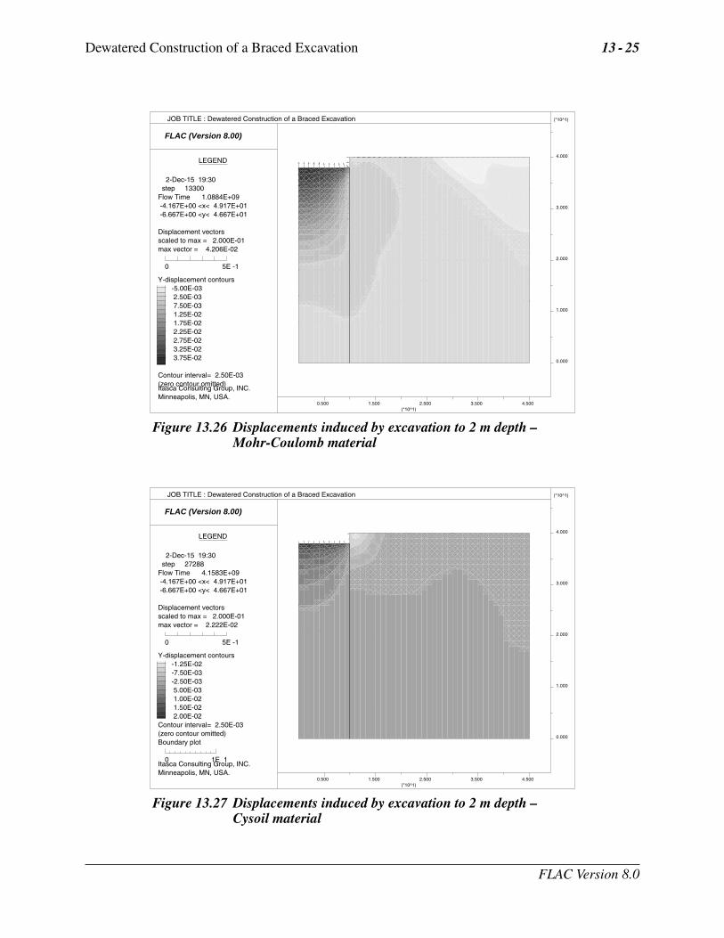
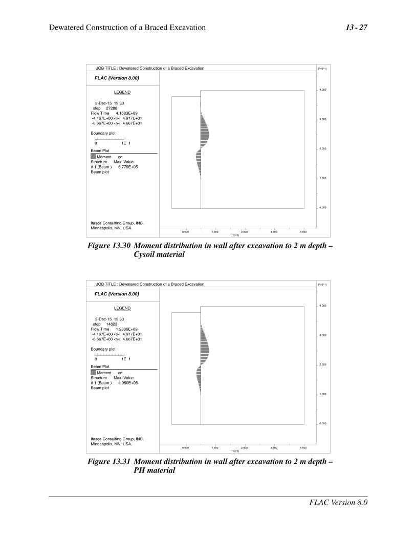
The displacements induced by this excavation are illustrated in Figure 13.26. A maximum heaveof roughly 4.2 cm occurs at the bottom of the excavation. We can also calculate the response ofthe wall. For example, the moment distribution in the wall after the first excavation is shown inFigure 13.29. Note that various results for the wall response (e.g., wall displacements, axial forces,shear forces) can be plotted using the Plot items dialog in the Plot/Model tool.

This step is now repeated with Cysoil material starting from “EXC03CY.SAV”. The displacementsinduced by this excavation stage are plotted in Figure 13.27 and indicate a maximum heave of

FLAC Version 8.0


roughly 2.2 cm. The moment distribution for this case is plotted in Figure 13.30; the maximumvalue is approximately 1.8 times that for the wall in Mohr-Coulomb material.

Figure 13.25 Excavated zones in the MaterialAssign tool

This step is repeated with the PH material starting with “EX04PH.SAV”. The displacements areplotted in Figure 13.28 and the wall moments in Figure 13.31.

FLAC Version 8.0


FLAC (Version 8.00)

LEGEND



0 5E -1

Y-displacement contours -5.00E-03 2.50E-03 7.50E-03 1.25E-02 1.75E-02 2.25E-02 2.75E-02 3.25E-02 3.75E-02

Contour interval= 2.50E-03(zero contour omitted)

0.000

1.000

2.000

3.000

4.000

(*10^1)

0.500 1.500 2.500 3.500 4.500(*10^1)



Figure 13.26 Displacements induced by excavation to 2 m depth –Mohr-Coulomb material

FLAC (Version 8.00)

LEGEND



0 5E -1

Y-displacement contours -1.25E-02 -7.50E-03 -2.50E-03 5.00E-03 1.00E-02 1.50E-02 2.00E-02 Contour interval= 2.50E-03(zero contour omitted)Boundary plot

0 1E 1

0.000

1.000

2.000

3.000

4.000

(*10^1)

0.500 1.500 2.500 3.500 4.500(*10^1)



Figure 13.27 Displacements induced by excavation to 2 m depth –Cysoil material

FLAC Version 8.0


FLAC (Version 8.00)

LEGEND



0 5E -1

Y-displacement contours -1.00E-02 -5.00E-03 2.50E-03 7.50E-03 1.25E-02 1.75E-02 2.25E-02 Contour interval= 2.50E-03(zero contour omitted)Boundary plot

0 1E 1

0.000

1.000

2.000

3.000

4.000

(*10^1)

0.500 1.500 2.500 3.500 4.500(*10^1)



Figure 13.28 Displacements induced by excavation to 2 m depth – PH material

FLAC (Version 8.00)

LEGEND


Boundary plot

0 1E 1

Beam Plot

Moment onStructure Max. Value# 1 (Beam ) 3.791E+05Beam plot

0.000

1.000

2.000

3.000

4.000

(*10^1)

0.500 1.500 2.500 3.500 4.500(*10^1)



Figure 13.29 Moment distribution in wall after excavation to 2 m depth –Mohr-Coulomb material

FLAC Version 8.0


FLAC (Version 8.00)

LEGEND


Boundary plot

0 1E 1

Beam Plot


0.000

1.000

2.000

3.000

4.000

(*10^1)

0.500 1.500 2.500 3.500 4.500(*10^1)



Figure 13.30 Moment distribution in wall after excavation to 2 m depth –Cysoil material

FLAC (Version 8.00)

LEGEND


Boundary plot

0 1E 1

Beam Plot


0.000

1.000

2.000

3.000

4.000

(*10^1)

0.500 1.500 2.500 3.500 4.500(*10^1)



Figure 13.31 Moment distribution in wall after excavation to 2 m depth –PH material

FLAC Version 8.0


13.2.6 Install Strut and Excavate to 10 m Depth

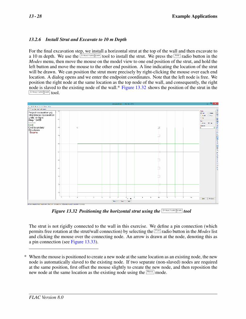
For the final excavation step, we install a horizontal strut at the top of the wall and then excavate toa 10 m depth. We use the StructureBeam tool to install the strut. We press the Add radio button in theModes menu, then move the mouse on the model view to one end position of the strut, and hold theleft button and move the mouse to the other end position. A line indicating the location of the strutwill be drawn. We can position the strut more precisely by right-clicking the mouse over each endlocation. A dialog opens and we enter the endpoint coordinates. Note that the left node is free. Weposition the right node at the same location as the top node of the wall, and consequently, the rightnode is slaved to the existing node of the wall.* Figure 13.32 shows the position of the strut in theStructureBeam tool.

Figure 13.32 Positioning the horizontal strut using the StructureBeam tool

The strut is not rigidly connected to the wall in this exercise. We define a pin connection (whichpermits free rotation at the strut/wall connection) by selecting the Pin radio button in the Modes listand clicking the mouse over the connecting node. An arrow is drawn at the node, denoting this asa pin connection (see Figure 13.33).

* When the mouse is positioned to create a new node at the same location as an existing node, the newnode is automatically slaved to the existing node. If two separate (non-slaved) nodes are requiredat the same position, first offset the mouse slightly to create the new node, and then reposition thenew node at the same location as the existing node using the Move mode.

FLAC Version 8.0


Figure 13.33 Selecting a pin connection in the StructureBeam tool

We also prescribe a different material property number to the strut in the Beam tool so that we canassign the strut properties. We click on the PropID radio button in the Modes list, and the identificationnumber B1 appears over the beam elements in the model plot. We click on the strut element, and adialog opens to allow us to rename the property ID to B2.

We now press Execute to send these commands to FLAC to create the strut, pin the strut to the walland assign the property number. Two nodes (32 and 33) are created, connected as a single beamelement and assigned property number 1002. A pin connection is defined between node 33 andwall node 2.

We enter the Structure / Node tool to assign fixity conditions for the strut. Node 33 is located alongthe centerline of the excavation. We click on this node to open a Node:33 dialog, as shown inFigure 13.34. We fix this node from movement in the x-direction, and from rotating (which areappropriate conditions for a node located along a line of symmetry), by clicking on the X-velocity

and Rotation check boxes in the dialog. We click OK and then Execute to send the node conditioncommands to FLAC.

FLAC Version 8.0


Figure 13.34 Node 33 dialog in the StructureNode tool

We assign the strut properties using the Structure/SEProp tool. We click on the strut element in thistool and open the Beam Element Properties dialog (as we did previously for the wall properties) toenter the strut properties as listed in Table 13.2.

We are now ready to perform the second excavation step. We use the MaterialAssign tool and change thezones within the range 0 ≤ x ≤ 10, 30 ≤ y ≤ 38 to null material. We press Run / Solve to calculatethe equilibrium state with this second excavation. We save this state as “EXC05MC.SAV”.

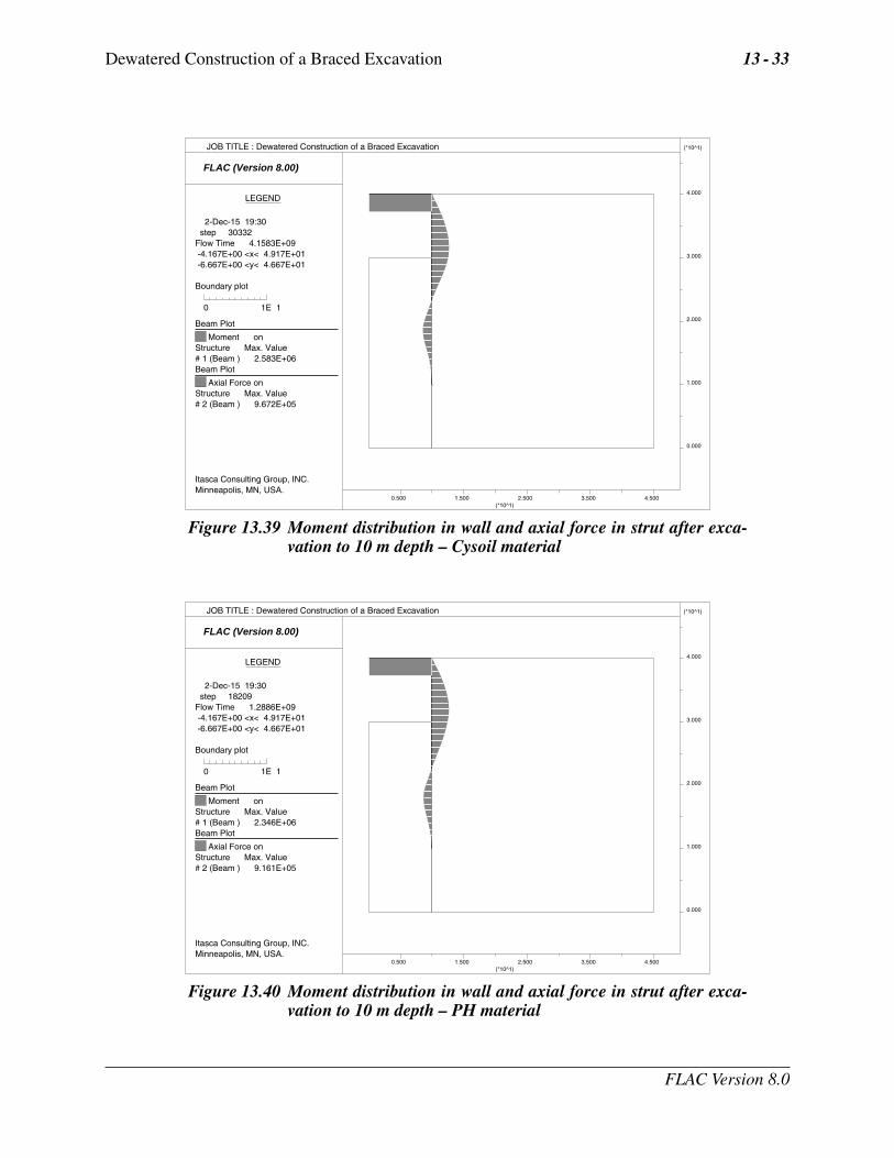
The total displacements induced by the excavation to the 10 m depth is illustrated in Figure 13.35;the moment distribution in the wall and axial force in the strut are shown in Figure 13.38.

This stage is repeated for Cysoil material and for PH material. The total displacements are plottedin Figure 13.36 for Cysoil material and in Figure 13.37 for PH material for comparison to the Mohr-Coulomb material. The maximum displacement at the bottom of the excavation is greater for theMohr-Coulomb material than for both Cysoil and PH materials. Also, the extent of the excavation-induced displacement is more confined than that for the Mohr-Coulomb material; compare they-displacement contour plot in Figures 13.36 and 13.37 to that in Figure 13.35.

The wall moments and strut load for Cysoil material are plotted in Figure 13.39 and for the PHmaterial in Figure 13.40. The values are roughly the same as those for Mohr-Coulomb material.

The surface settlement and the wall deflection are also compared for the three soil types. Figure 13.41plots surface settlement and shows roughly the same settlement profiles for all three material models.Figure 13.42 plots the wall deflection. The Mohr-Coulomb material results in higher deflections.Deflections resulting from Cysoil and PH materials match quite closely.

FLAC Version 8.0


FLAC (Version 8.00)

LEGEND



0 5E -1

Y-displacement contours -7.50E-02 -2.50E-02 5.00E-02 1.00E-01 1.50E-01 2.00E-01 Contour interval= 2.50E-02(zero contour omitted)Boundary plot

0 1E 1

0.000

1.000

2.000

3.000

4.000

(*10^1)

0.500 1.500 2.500 3.500 4.500(*10^1)



Figure 13.35 Displacements induced by excavation to 10 m depth –Mohr-Coulomb material

FLAC (Version 8.00)

LEGEND



0 5E -1

Y-displacement contours -9.00E-02 -7.00E-02 -5.00E-02 -3.00E-02 -1.00E-02 2.00E-02 4.00E-02 6.00E-02 8.00E-02 Contour interval= 1.00E-02(zero contour omitted)Boundary plot

0.000

1.000

2.000

3.000

4.000

(*10^1)

0.500 1.500 2.500 3.500 4.500(*10^1)



Figure 13.36 Displacements induced by excavation to 10 m depth –Cysoil material

FLAC Version 8.0


FLAC (Version 8.00)

LEGEND



0 5E -1

Y-displacement contours -8.00E-02 -5.00E-02 -2.00E-02 2.00E-02 5.00E-02 8.00E-02 1.10E-01 Contour interval= 1.00E-02(zero contour omitted)Boundary plot

0 1E 1

0.000

1.000

2.000

3.000

4.000

(*10^1)

0.500 1.500 2.500 3.500 4.500(*10^1)



Figure 13.37 Displacements induced by excavation to 10 m depth – PH material

FLAC (Version 8.00)

LEGEND


Boundary plot

0 1E 1

Beam Plot

Moment onStructure Max. Value# 1 (Beam ) 2.606E+06Beam Plot

Axial Force onStructure Max. Value# 2 (Beam ) 1.009E+06

0.000

1.000

2.000

3.000

4.000

(*10^1)

0.500 1.500 2.500 3.500 4.500(*10^1)



Figure 13.38 Moment distribution in wall and axial force in strut after exca-vation to 10 m depth – Mohr-Coulomb material

FLAC Version 8.0


FLAC (Version 8.00)

LEGEND


Boundary plot

0 1E 1

Beam Plot



0.000

1.000

2.000

3.000

4.000

(*10^1)

0.500 1.500 2.500 3.500 4.500(*10^1)



Figure 13.39 Moment distribution in wall and axial force in strut after exca-vation to 10 m depth – Cysoil material

FLAC (Version 8.00)

LEGEND


Boundary plot

0 1E 1

Beam Plot



0.000

1.000

2.000

3.000

4.000

(*10^1)

0.500 1.500 2.500 3.500 4.500(*10^1)



Figure 13.40 Moment distribution in wall and axial force in strut after exca-vation to 10 m depth – PH material

FLAC Version 8.0


FLAC (Version 8.00)

LEGEND

2-Dec-15 19:30 step 0 Table PlotMohr-Coulomb

Cysoil

PH

15 20 25 30 35 40 45

-9.000

-8.000

-7.000

-6.000

-5.000

-4.000

-3.000

-2.000

-1.000

0.000

(10 )-02



Figure 13.41 Surface settlement profiles

FLAC (Version 8.00)

LEGEND

2-Dec-15 19:30 step 0 Table PlotMohr-Coulomb

Cysoil

PH

-14 -12 -10 -8 -6 -4 -2

(10 )-02

1.500

2.000

2.500

3.000

3.500

4.000

(10 ) 01



Figure 13.42 Wall deflection

FLAC Version 8.0


13.3 Observations

This example illustrates the effect of the material model on soil deformational response for unloadingproblems such as the construction on a braced excavation. The heave that occurs at the bottom ofthe excavation is considerably greater for the construction in Mohr-Coulomb material than it is forCysoil material or PH material. This is primarily attributed to the stress-dependent elastic moduliand stiffer unloading response of the Cysoil and PH materials. This is evident from the comparisonof the displacement contour plots in Figure 13.35 for the Mohr-Coulomb material, and Figure 13.36for the Cysoil material and Figure 13.37 for PH material.

This model example was derived for comparison to the excavation example with Mohr-Coulombmaterial and hardening soil material given in the Plaxis Material Models Manual (2002). A qual-itative agreement with those results is shown here. This example illustrates a procedure to matchproperties between the Cysoil and PH materials. Also, see Section 17 for a comparison betweenthe Cysoil model, the PH model and the hardening soil model in a field benchmark study.

13.4 References

Plaxis BV. PLAXIS Version 8, Material Models Manual. R.B.J. Brinkgreve, ed. Delft: Plaxis(2002).

Plaxis BV. PLAXIS Version 8, Tutorial Manual. R.B.J. Brinkgreve, ed. Delft: Plaxis (2002).

FLAC Version 8.0


FLAC Version 8.0

13 dewatered construction of a braced...

Documents