12. the wave equation vibrating finite stringggeorge/4430/handout/h12pde_fou… · ·...

ENGI 4430 PDEs - Fourier Solutions 2.01

12. The Wave Equation – Vibrating Finite String

The wave equation is 2

2 2

2

uc u

t

If ,u x t is the vertical displacement of a point at location x on a vibrating string at

time t, then the governing PDE is 2 2

2

2 2

u uc

t x

If , ,u x y t is the vertical displacement of a point at location ,x y on a vibrating

membrane at time t, then the governing PDE is 2 2 2

2

2 2 2

u u uc

t x y

or, in plane polar coordinates ,r , (appropriate for a circular drum),

2 2 22

2 2 2 2

1 1u u u uc

t r r r r

Example 12.01

An elastic string of length L is fixed at both ends 0 andx x L . The string is

displaced into the form y f x and is released from rest. Find the displacement

,y x t at all locations on the string 0 x L and at all subsequent times 0t .

The boundary value problem for the displacement function ,y x t is:

2 2

2

2 2for 0 and 0

y yc x L t

t x

Both ends fixed for all time:

Initial configuration of string:

String released from rest:

ENGI 4430 PDEs - Fourier Solutions Page 12.02

Example 12.01 (continued)

Separation of Variables (or Fourier Method)

Attempt a solution of the form ,y x t X x T t

Substitute ,y x t X x T t into the PDE:

2 2 2 2

2 2

2 2 2 2

d T d XX x T t c X x T t X c T

t x dt dx

2 2

2 2 2

1 1 1d T d X

c T dt X dx



Therefore our complete solution is

0

1

2, sin sin cos

L

n

n u n x n cty x t f u du

L L L L



This solution is valid for any initial displacement function f x that is continuous with a

piece-wise continuous derivative on 0, L with 0 0f f L .

If the initial displacement is itself sinusoidal sin for somen x

f x a nL

,

then the complete solution is a single term from the infinite series,

, sin cosn x n ct

y x t aL L

.

Suppose that the initial configuration is triangular:

12

12

0,0

x x Ly x f x

L x L x L

Then the Fourier sine coefficients are

0

2sin

L

nn u

C f u duL L



See the web page "www.engr.mun.ca/~ggeorge/4430/demos/ex1201.html" for

an animation of this solution.



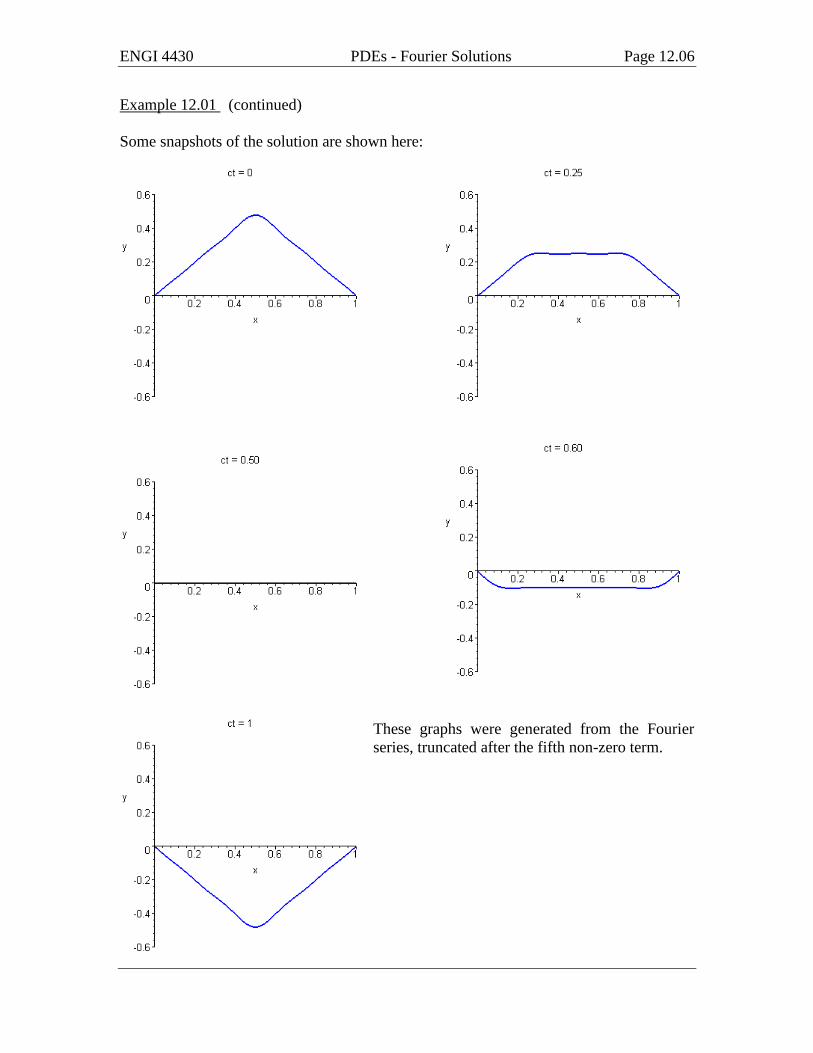
Some snapshots of the solution are shown here:

These graphs were generated from the Fourier

series, truncated after the fifth non-zero term.


Example 12.02

An elastic string of length L is fixed at both ends 0 andx x L . The string is

initially in its equilibrium state [ ,0 0y x for all x] and is released with the initial

velocity

,0x

yg x

t

. Find the displacement ,y x t at all locations on the string

0 x L and at all subsequent times 0t .

The boundary value problem for the displacement function ,y x t is:

2 2

2

2 2for 0 and 0

y yc x L t

t x

Both ends fixed for all time: 0, , 0 for 0y t y L t t

Initial configuration of string: ,0 0 for 0y x x L

String released with initial velocity:

,0

for 0

x

yg x x L

t

As before, attempt a solution by the method of the separation of variables.

Substitute ,y x t X x T t into the PDE:

2 2 2 2

2 2

2 2 2 2

d T d XX x T t c X x T t X c T

t x dt dx

Again, each side must be a negative constant. 2 2

2

2 2 2

1 1d T d X

c T dt X dx

We now have the pair of ODEs 2 2

2 2 2

2 20 and 0

d X d TX c T

dx dt

The general solutions are

cos sin and cos sinX x A x B x T t C ct D ct

respectively, where A, B, C and D are arbitrary constants.



Consider the boundary conditions:

0, 0 0 0y t X T t t

For a non-trivial solution, this requires 0 0 0X A .

, 0 0 0y L t X L T t t X L

sin 0 ,nn

B L nL

We now have a solution only for a discrete set of eigenvalues n , with corresponding

eigenfunctions

sin , 1, 2, 3,nn x

X x nL

and

, sin , 1, 2, 3,n n n nn x

y x t X x T t T t nL

So far, the solution has been identical to Example 12.01.

Consider the initial condition ,0 0y x :

,0 0 0 0 0 0y x X x T x T

The initial value problem for T t is now

2 2 0 , 0 0 , wheren

T c T TL

the solution to which is

sin ,n nn ct

T t C nL

Our eigenfunctions for y are now

, sin sin ,n n n nn x n ct

y x t X x T t C nL L



Differentiate term by term and impose the initial velocity condition:

, 0 1

sin

x

n

n

y n c n xC g x

t L L

which is just the Fourier sine series expansion for the function g x .

The coefficients of the expansion are

0

2sin

L

nn c n u

C g u duL L L

which leads to the complete solution

0

1

2 1, sin sin sin

L

n

n u n x n cty x t g u du

c n L L L

This solution is valid for any initial velocity function g x that is continuous with a

piece-wise continuous derivative on [0, L] with 0 0g g L .

The solutions for Examples 12.01 and 12.02 may be superposed.

Let 1 ,y x t be the solution for initial displacement f x and zero initial velocity.

Let 2 ,y x t be the solution for zero initial displacement and initial velocity g x .

Then 1 2, , ,y x t y x t y x t satisfies the wave equation

(the sum of any two solutions of a linear homogeneous PDE is also a solution),

and satisfies the boundary conditions 0, , 0y t y L t .

1 2,0 ,0 ,0 0 ,y x y x y x f x

which satisfies the condition for initial displacement f x .

1 2,0 ,0 ,0 0 ,t t ty x y x y x g x

which satisfies the condition for initial velocity g x .

Therefore the sum of the two solutions is the complete solution for initial displacement

f x and initial velocity g x :

0

0

1

1

2, sin sin cos

2 1sin sin sin

L

L

n

n

n u n x n c ty x t f u du

L L L L

n u n x n c tg u du

c n L L L


The Heat Equation

For a material of constant density , constant specific heat and constant thermal

conductivity K, the partial differential equation governing the temperature u at any

location , ,x y z and any time t is

2 , whereu K

k u kt

Example 12.03

Heat is conducted along a thin homogeneous bar extending from x = 0 to x = L. There is

no heat loss from the sides of the bar. The two ends of the bar are maintained at

temperatures 1T (at x = 0) and 2T (at x = L). The initial temperature throughout the bar

at the cross-section x is f x .

Find the temperature at any point in the bar at any subsequent time.

The partial differential equation governing the temperature ,u x t in the bar is

2

2

u uk

t x

together with the boundary conditions

10,u t T and 2,u L t T

and the initial condition

,0u x f x

[Note that if an end of the bar is insulated, instead of being maintained at a constant

temperature, then the boundary condition changes to 0, 0u

tt

or , 0

uL t

t

.]

Attempt a solution by the method of separation of variables.

,u x t X x T t

T XX T k X T k c

T X

Again, when a function of t only equals a function of x only, both functions must equal

the same absolute constant. Unfortunately, the two boundary conditions cannot both be

satisfied unless 1 2 0T T . Therefore we need to treat this more general case as a

perturbation of the simpler 1 2 0T T case.



Let , ,u x t v x t g x

Substitute this into the PDE:

2 2

2 2, ,

v vv x t g x k v x t g x k g x

t x t x

This is the standard heat PDE for v if we choose g such that 0g x .

g x must therefore be a linear function of x.

We want the perturbation function g x to be such that

10,u t T , 2,u L t T

and

0, , 0v t v L t

Therefore g x must be the linear function for which 10g T and 2g L T . It

follows that

2 11

T Tg x x T

L

and we now have the simpler problem

2

2

v vk

t x

together with the boundary conditions

0, , 0v t v L t

and the initial condition

,0v x f x g x

Now try separation of variables on ,v x t :

,v x t X x T t 1 T X

X T k X T ck T X

But 0, , 0 0 0v t v L t X X L

This requires c to be a negative constant, say 2 .

The solution is very similar to that for the wave equation on a finite string with fixed ends

(examples 12.01 and 12.02). The eigenvalues are n

L

and the corresponding

eigenfunctions are any non-zero constant multiples of

sinnn x

X xL

ENGI 4430 PDEs - Fourier Solutions .12


The ODE for T t is first order:

2

0n

T k TL

whose general solution is

2 2 2/n kt L

n nT t c e

Therefore

2 2

2, sin expn n n n

n x n ktv x t X x T t c

L L

If the initial temperature distribution f x g x is a simple multiple of sinn x

L

for

some integer n, then the solution for v is just 2 2

2, sin expn

n x n ktv x t c

L L

.

Otherwise, we must attempt a superposition of solutions.

2 2

2

1

, sin expn

n

n x n ktv x t c

L L

such that 1

,0 sinn

n

n xv x c f x g x

L

.

The Fourier sine series coefficients are 0

2sinn

Ln z

c f z g z dzL L

so that the complete solution for ,v x t is

2 2

2 11 2

01

2, sin sin exp

L

n

T T n z n x n ktv x t f z z T dz

L L L L L

and the complete solution for ,u x t is

2 11, ,

T Tu x t v x t x T

L

Note how this solution can be partitioned into a transient part ,v x t (which decays to

zero as t increases) and a linear steady-state part g x which is the limiting value that the

temperature distribution approaches.



As a specific example, let 1 29, 100, 200, 2k T T L and

2145 240 100f x x x , (for which 0 100, 2 200f f and 0f x x ).

Then 200 100

100 50 1002

g x x x

The Fourier sine series coefficients are

The complete solution is

2 2

3 3

1

1 12320 9, 50 100 sin exp

2 4

n

n

n x n tu x t x

n

Some snapshots of the temperature distribution (from the tenth partial sum) from the

Maple file at "www.engr.mun.ca/~ggeorge/4430/demos/ex1205.mws" are shown

on the next page.



The steady state distribution is nearly attained in much less than a second!


Example 12.04

A perfectly elastic string of equilibrium length 4 metres is released from rest in a

trapezoidal configuration shown here:

The string is clamped at both ends (x = 0 and x = 4).

Waves move on the string with speed c. There is no friction.

Determine the subsequent evolution of the displacement ,y x t of the string.

The initial displacement is

0 1

1 1 3,0

4 3 4

0 otherwise

x x

xy x f x

x x

The coefficients in the Fourier sine series for ,y x t are

4

0

sin4

nn u

c f u du

However the integrand changes its functional form abruptly at x = 1 and again at x = 3.

The integral must therefore be split into three pieces:

1 3 4

0 1 3

sin 1sin 4 sin4 4 4

nn u n u n u

c u du du u du

Using integrations by parts on the first and last integrals,

2

2

1

0

3

1

4

3

4 4cos sin

4 4

4cos

4

4 44 cos sin

4 4

nn u n u

c un n

n u

n

n u n uu

n n



4cos

4n

nc

n

2

4sin 0 0

4

4 3cos

4

n

n

n

n

4cos

4

n

n

4 30 0 cos

4

n

n

2

4 3sin

4

n

n

2 2

4 3 4sin sin 2 sin cos

4 4 2 4n

n n n nc

n n

(using the trigonometric identity sin sin 2sin cos2 2

A B A BA B

)

This series has a fairly rapid convergence: it is of the form 2

1

n with 0nc for all even n.

Substituting into the complete solution of the wave PDE, we have

2 2

1

16 1, sin cos sin cos

2 4 4 4n

n n n x n cty x t

n

An animation of the solution and a Maple file are available from the course web site, at

" www.engr.mun.ca/~ggeorge/4430/demos/ex1206.html ".

Two snapshots (from the sum of the first six non-trivial terms in the series) are shown

here.

0t 1.6ct


Example 12.05

A perfectly elastic string of equilibrium length 10 metres is released from rest in a

configuration very close to that of a square pulse of unit height, between x = 5 and x = 6,

that is

1 5 6,0

0 otherwise

xy x f x

The string is clamped at both ends (x = 0 and x = 10).



First let us anticipate the response.

The initial configuration looks like this. The pulse is just to the right of the centre of the

string.

Two copies of the initial configuration, each half the height of the original, move off in

opposite directions.

If the string were infinite, then the two waves would continue to recede from each other

forever. At the fixed ends of the string, the waves bounce back, reflected.

They travel towards each other until they recombine into the negative of the original

wave, just to the left of the centre of the string.

The second half of the cycle looks like a time-reversed version of the first half.



The general solution of the wave equation

2 2

2

2 2for 0 and 0

y yc x L t

t x

with conditions

Both ends fixed for all time: 0, , 0 for 0y t y L t t

Initial configuration of string: ,0 for 0y x f x x L

String released from rest:

,0

0 for 0

x

yx L

t

is the Fourier series

01

2, sin sin cos

L

n

n u n x n cty x t f u du

L L L L

Here L = 10 and

1 5 6,0

0 otherwise

xy x f x

0 5

610 6

5

10sin 0 1sin 0 cos

10 10 10

n u n u n uf u du du

n

10 6 5 10 3cos cos cos cos

10 10 2 5

n n n n

n n

1

2 1 3, cos cos sin cos

2 5 10 10n

n n n x n cty x t

n

This series is very slow to converge (which is no surprise, given that f x is not even

continuous, let alone differentiable, in two places).



The animation of the solution uses the partial sum of the first thirty terms of the Fourier

series. Even with this large number of terms, the approximation is quite rough. Some

snapshots are shown on the next page.



t = 0 ct = 3.5

ct = 6.5 ct = 10.0


Example 12.06

A perfectly elastic string of equilibrium length L is released from the initial shape

2

,0 sinx

y x f xL

with an initial velocity profile

4

,0 sintx

y x g xL

The string is clamped at both ends (x = 0 and x = L).



The trigonometric identity 2sin sin cos cosA B A B A B can be used to

verify the orthogonality property of the set of sine functions sinn x

L

on [0, L]:

0

12sin sin

0 otherwise

L m nm u n udu

L L L

Therefore in the complete solution of the wave equation

0

0

1

1

2, sin sin cos

2 1sin sin sin

L

n

L

n

n u n x n c ty x t f u du

L L L L

n u n x n c tg u du

c n L L L

only the n = 2 term is non-zero in the first series and

only the n = 4 term is non-zero in the second series.

The complete solution reduces to

2 2 4 4

, sin cos sin sin4

x ct L x cty x t

L L c L L



[End of Chapter 12]

END OF ENGI 4430!

12. the wave equation vibrating finite stringggeorge/4430/handout/h12pde_fou… · ·...

Documents