1

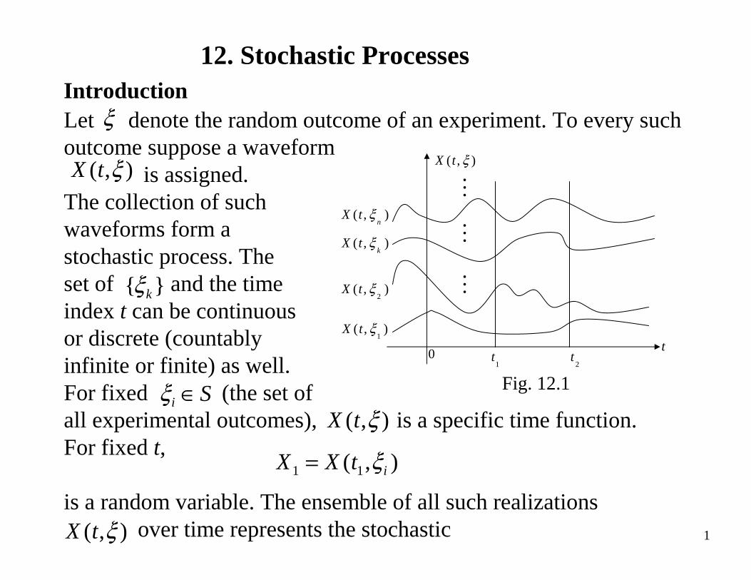
Let denote the random outcome of an experiment. To every such outcome suppose a waveform

is assigned.The collection of such waveforms form a stochastic process. The set of and the time index t can be continuousor discrete (countably infinite or finite) as well.For fixed (the set of all experimental outcomes), is a specific time function.For fixed t,

is a random variable. The ensemble of all such realizationsover time represents the stochastic

ξ

),( ξtX

}{ kξ

Si ∈ξ

),( 11 itXX ξ=

),( ξtX

12. Stochastic Processes

t1

t2

t

),(n

tX ξ

),(k

tX ξ

),(2

ξtX

),(1

ξtX

Fig. 12.1

),( ξtX

0

),( ξtX

Introduction

2

process X(t). (see Fig 12.1). For example

where is a uniformly distributed random variable in represents a stochastic process. Stochastic processes are everywhere:Brownian motion, stock market fluctuations, various queuing systemsall represent stochastic phenomena.

If X(t) is a stochastic process, then for fixed t, X(t) representsa random variable. Its distribution function is given by

Notice that depends on t, since for a different t, we obtaina different random variable. Further

represents the first-order probability density function of the process X(t).

),cos()( 0 ϕω += tatX

ϕ

})({),( xtXPtxFX

≤=

),( txFX

(12-1)

(12-2)

(0,2 ),π

dx

txdFtxf X

X

),(),( =∆

3

For t = t1 and t = t2, X(t) represents two different random variablesX1 = X(t1) and X2 = X(t2) respectively. Their joint distribution is given by

and

represents the second-order density function of the process X(t).Similarly represents the nth order densityfunction of the process X(t). Complete specification of the stochasticprocess X(t) requires the knowledge of for all and for all n. (an almost impossible taskin reality).

})(,)({),,,( 22112121 xtXxtXPttxxFX

≤≤= (12-3)

(12-4)

),, ,,,( 2121 nn tttxxxfX

),, ,,,( 2121 nn tttxxxfX

niti , ,2 ,1 , =

21 2 1 2

1 2 1 21 2

( , , , )( , , , )

X

X

F x x t tf x x t t

x x

∂=

∂ ∂∆

4

Mean of a Stochastic Process:

represents the mean value of a process X(t). In general, the mean of a process can depend on the time index t.

Autocorrelation function of a process X(t) is defined as

and it represents the interrelationship between the random variablesX1 = X(t1) and X2 = X(t2) generated from the process X(t).

Properties:

1.

2.

(12-5)

(12-6)

*1

*212

*21 )}]()({[),(),( tXtXEttRttR

XXXX== (12-7)

.0}|)({|),( 2 >= tXEttRXX

(Average instantaneous power)

( ) { ( )} ( , )

Xt E X t x f x t dxµ +∞

−∞= = ∫∆

* *1 2 1 2 1 2 1 2 1 2 1 2( , ) { ( ) ( )} ( , , , )

XX XR t t E X t X t x x f x x t t dx dx= = ∫ ∫

∆

5

3. represents a nonnegative definite function, i.e., for anyset of constants

Eq. (12-8) follows by noticing that The function

represents the autocovariance function of the process X(t).Example 12.1Let

Then

.)(for 0}|{|1

2 ∑=

=≥n

iii tXaYYE

)()(),(),( 2*

12121 ttttRttCXXXXXX

µµ−= (12-9)

.)(

∫−=

T

TdttXz

∫ ∫

∫ ∫

− −

− −

=

=T

T

T

T

T

T

T

T

dtdtttR

dtdttXtXEzE

XX

2121

212*

12

),(

)}()({]|[|

(12-10)

niia 1}{ =

),( 21 ttRXX

∑∑= =

≥n

i

n

jjiji ttRaa

XX

1 1

* .0),( (12-8)

6

Similarly

,0}{sinsin}{coscos

)}{cos()}({)(

0 0

0

=−=+==

ϕωϕωϕωµ

EtaEta

taEtXEtX

).(cos2

)}2)(cos()({cos2

)}cos(){cos(),(

210

2

210210

2

20102

21

tta

ttttEa

ttEattRXX

−=

+++−=

++=

ω

ϕωω

ϕωϕω

(12-12)

(12-13)

Example 12.2

).2,0(~ ),cos()( 0 πϕϕω UtatX += (12-11)

This gives

∫ ===π ϕϕϕϕ π

2

0 }.{sin0cos}{cos since 2

1 EdE

7

Stationary Stochastic ProcessesStationary processes exhibit statistical properties that are

invariant to shift in the time index. Thus, for example, second-orderstationarity implies that the statistical properties of the pairs {X(t1) , X(t2) } and {X(t1+c) , X(t2+c)} are the same for any c. Similarly first-order stationarity implies that the statistical properties of X(ti) and X(ti+c) are the same for any c.

In strict terms, the statistical properties are governed by thejoint probability density function. Hence a process is nth-orderStrict-Sense Stationary (S.S.S) if

for any c, where the left side represents the joint density function of the random variables andthe right side corresponds to the joint density function of the randomvariables A process X(t) is said to be strict-sense stationary if (12-12) is true for all

),, ,,,(),, ,,,( 21212121 ctctctxxxftttxxxf nnnn XX+++≡

(12-12)

)( , ),( ),( 2211 nn tXXtXXtXX ===

).( , ),( ),( 2211 ctXXctXXctXX nn +=′+=′+=′

. and ,2 ,1 , , ,2 ,1 , canynniti ==

8

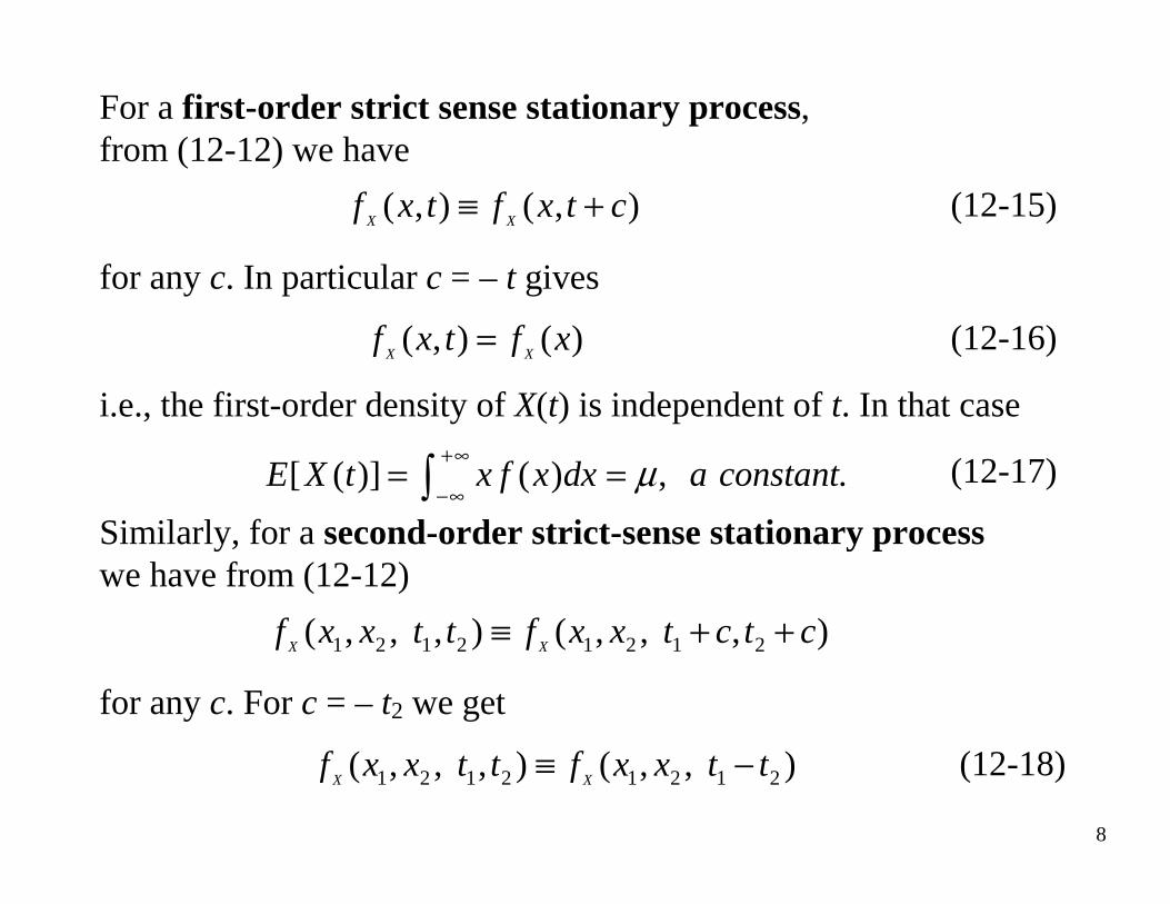
For a first-order strict sense stationary process,from (12-12) we have

for any c. In particular c = – t gives

i.e., the first-order density of X(t) is independent of t. In that case

Similarly, for a second-order strict-sense stationary processwe have from (12-12)

for any c. For c = – t2 we get

),(),( ctxftxfXX

+≡

(12-16)

(12-15)

(12-17)

)(),( xftxfXX

=

[ ( )] ( ) , E X t x f x dx a constant.µ+∞

−∞= =∫

), ,,(), ,,( 21212121 ctctxxfttxxfXX

++≡

) ,,(), ,,( 21212121 ttxxfttxxfXX

−≡ (12-18)

9

i.e., the second order density function of a strict sense stationary process depends only on the difference of the time indices In that case the autocorrelation function is given by

i.e., the autocorrelation function of a second order strict-sensestationary process depends only on the difference of the time indices Notice that (12-17) and (12-19) are consequences of the stochastic process being first and second-order strict sense stationary. On the other hand, the basic conditions for the first and second order stationarity – Eqs. (12-16) and (12-18) – are usually difficult to verify.In that case, we often resort to a looser definition of stationarity,known as Wide-Sense Stationarity (W.S.S), by making use of

.21 τ=− tt

.21 tt −=τ

(12-19)

*1 2 1 2

*1 2 1 2 1 2 1 2

*1 2

( , ) { ( ) ( )}

( , , )

( ) ( ) ( ),

XX

X

XX XX XX

R t t E X t X t

x x f x x t t dx dx

R t t R R

τ

τ τ

=

= = −

= − = = −∫ ∫

∆

∆

10

(12-17) and (12-19) as the necessary conditions. Thus, a process X(t)is said to be Wide-Sense Stationary if(i)and(ii)

i.e., for wide-sense stationary processes, the mean is a constant and the autocorrelation function depends only on the difference between the time indices. Notice that (12-20)-(12-21) does not say anything about the nature of the probability density functions, and instead deal with the average behavior of the process. Since (12-20)-(12-21) follow from (12-16) and (12-18), strict-sense stationarity always implies wide-sense stationarity. However, the converse is not true in general, the only exception being the Gaussian process.This follows, since if X(t) is a Gaussian process, then by definition

are jointly Gaussian randomvariables for any whose joint characteristic function is given by

µ=)}({ tXE

(12-21)

(12-20)

),()}()({ 212*

1 ttRtXtXEXX

−=

)( , ),( ),( 2211 nn tXXtXXtXX ===nttt ,, 21

11

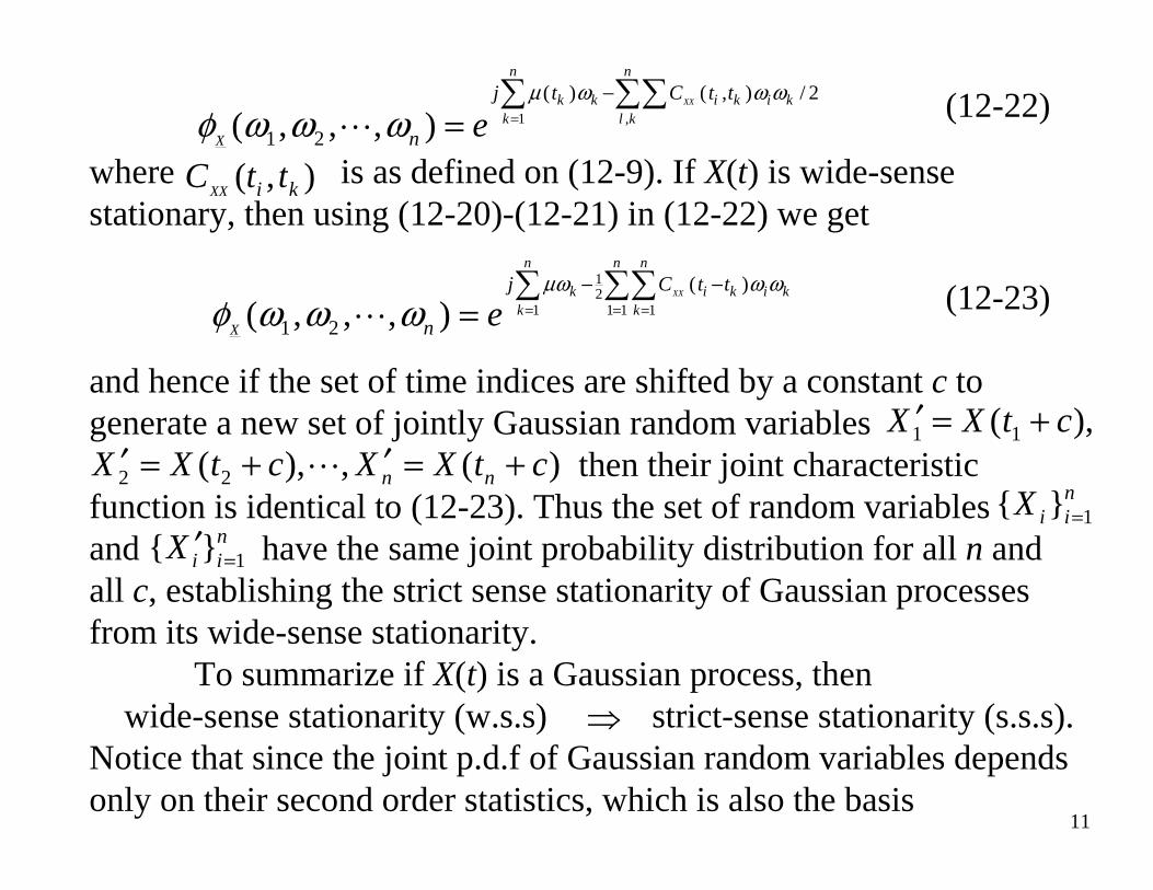
where is as defined on (12-9). If X(t) is wide-sense stationary, then using (12-20)-(12-21) in (12-22) we get

and hence if the set of time indices are shifted by a constant c to generate a new set of jointly Gaussian random variables

then their joint characteristic function is identical to (12-23). Thus the set of random variables and have the same joint probability distribution for all n and all c, establishing the strict sense stationarity of Gaussian processes from its wide-sense stationarity.

To summarize if X(t) is a Gaussian process, thenwide-sense stationarity (w.s.s) strict-sense stationarity (s.s.s).

Notice that since the joint p.d.f of Gaussian random variables dependsonly on their second order statistics, which is also the basis

),( ki ttCXX

1 ,

( ) ( , ) / 2

1 2( , , , )XX

n n

k k i k i kk l k

X

j t C t t

n eµ ω ω ω

φ ω ω ω =

−∑ ∑∑= (12-22)

12

1 1 1 1

( )

1 2( , , , )XX

n n n

k i k i kk k

X

j C t t

n eµω ω ω

φ ω ω ω = = =

− −∑ ∑∑= (12-23)

niiX 1}{ =

niiX 1}{ =′

⇒

),( 11 ctXX +=′)(,),( 22 ctXXctXX nn +=′+=′

12

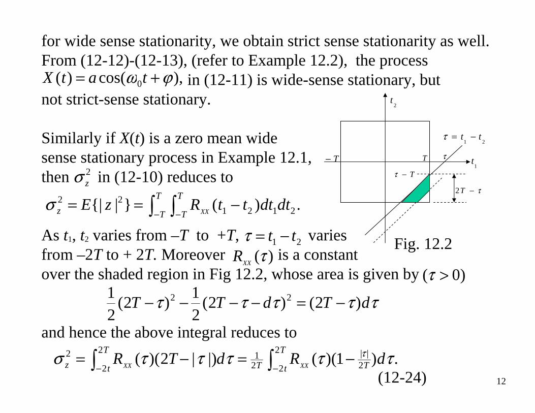
for wide sense stationarity, we obtain strict sense stationarity as well.From (12-12)-(12-13), (refer to Example 12.2), the process

in (12-11) is wide-sense stationary, butnot strict-sense stationary.

Similarly if X(t) is a zero mean wide sense stationary process in Example 12.1, then in (12-10) reduces to

As t1, t2 varies from –T to +T, variesfrom –2T to + 2T. Moreover is a constantover the shaded region in Fig 12.2, whose area is given by

and hence the above integral reduces to

),cos()( 0 ϕω += tatX

2zσ

.)(}|{|

212122 ∫ ∫− −

−==T

T

T

Tz dtdtttRzEXX

σ

21 tt −=τ)(τ

XXR

)0( >ττττττ dTdTT )2()2(

21

)2(21 22 −=−−−−

.)1)((|)|2)((2

2 2||

21

2

2

2 ∫∫ −−−=−=

T

t TT

T

tz dRdTRXXXX

τττττσ τ

(12-24)

T− T

T−τ

τ

τ−T2

2t

1t

Fig. 12.2

21tt −=τ

13

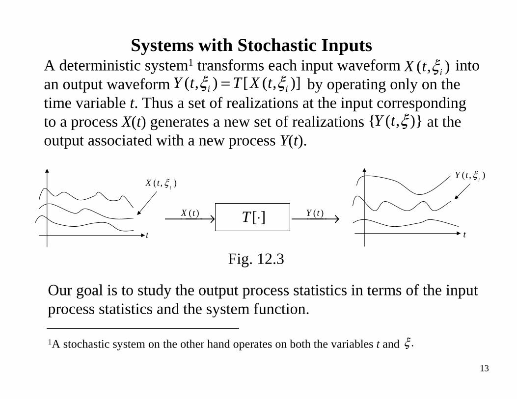
Systems with Stochastic InputsA deterministic system1 transforms each input waveform intoan output waveform by operating only on the time variable t. Thus a set of realizations at the input corresponding to a process X(t) generates a new set of realizations at the output associated with a new process Y(t).

),( itX ξ)],([),( ii tXTtY ξξ =

)},({ ξtY

Our goal is to study the output process statistics in terms of the inputprocess statistics and the system function.

1A stochastic system on the other hand operates on both the variables t and .ξ

][⋅T⎯⎯ →⎯ )(tX ⎯⎯→⎯ )(tY

t t

),(i

tX ξ),(

itY ξ

Fig. 12.3

14

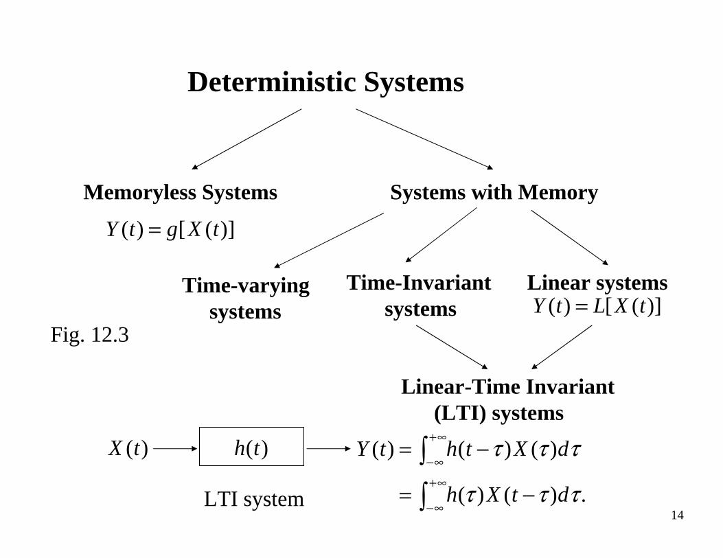
Deterministic Systems

Systems with Memory

Time-Invariantsystems

Linear systems

Linear-Time Invariant(LTI) systems

Memoryless Systems

)]([)( tXgtY =

)]([)( tXLtY =Time-varying

systemsFig. 12.3

.)()(

)()()(

∫

∫∞+

∞−

∞+

∞−

−=

−=

τττ

τττ

dtXh

dXthtY( )h t( )X t

LTI system

15

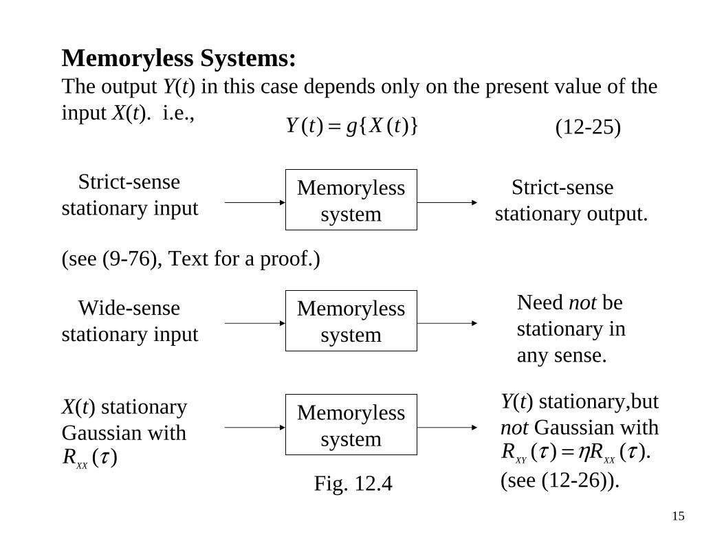
Memoryless Systems:The output Y(t) in this case depends only on the present value of the input X(t). i.e.,

(12-25))}({)( tXgtY =

Memorylesssystem

Memorylesssystem

Memorylesssystem

Strict-sense stationary input

Wide-sense stationary input

X(t) stationary Gaussian with

)(τXX

R

Strict-sense stationary output.

Need not bestationary in any sense.

Y(t) stationary,butnot Gaussian with

(see (12-26)).).()( τητ

XXXYRR =

(see (9-76), Text for a proof.)

Fig. 12.4

16

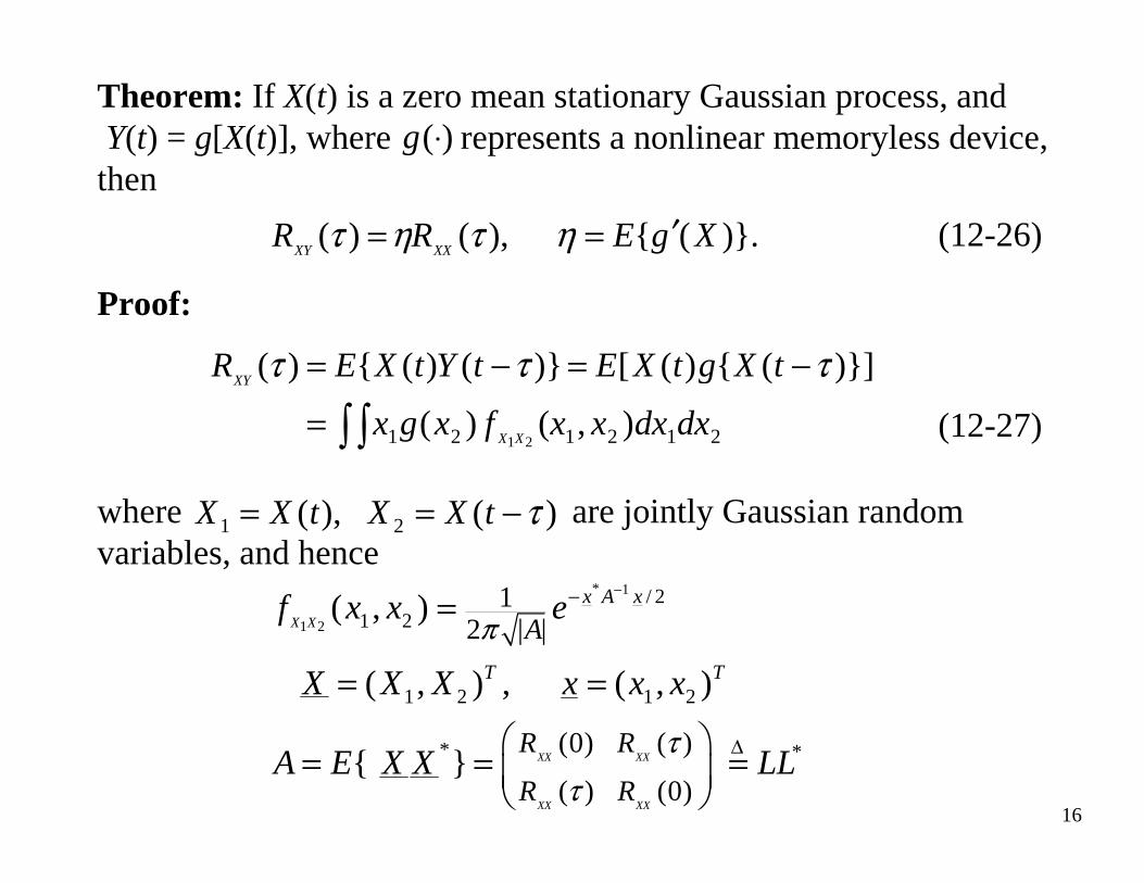
Theorem: If X(t) is a zero mean stationary Gaussian process, andY(t) = g[X(t)], where represents a nonlinear memoryless device, then

Proof:

where are jointly Gaussian random variables, and hence

)(⋅g

)}.({ ),()( XgERRXXXY

′== ητητ (12-26)

212121 ),()(

)}]({)([)}()({)(

21dxdxxxfxgx

tXgtXEtYtXER

XX

XY

∫ ∫=

−=−= τττ

(12-27)

)( ),( 21 τ−== tXXtXX

* 1

1 2

/ 21 2

1 2 1 2

* *

12 | |

(0) ( )

( ) (0)

( , )

( , ) , ( , )

{ } XX XX

XX XX

X X

x A x

T T

A

R R

R R

f x x e

X X X x x x

A E X X LL

π

ττ

−−=

= =

⎛ ⎞= = =⎜ ⎟⎝ ⎠

∆

17

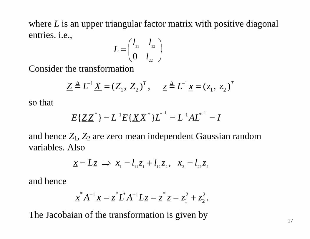
where L is an upper triangular factor matrix with positive diagonal entries. i.e.,

Consider the transformation

so that

and hence Z1, Z2 are zero mean independent Gaussian random variables. Also

and hence

The Jacobaian of the transformation is given by

. 0

22

1211 ⎟⎠

⎞⎜⎝

⎛=l

llL

IALLLXXELZZE ===−− −− 11 *1**1* }{}{

* * *1 * 1 2 21 2 .x A x z L A Lz z z z z− −= = = +

22222121111 , zlxzlzlxzLx =+=⇒=

1 1 1 2 1 2( , ) , ( , )T TZ L X Z Z z L x z z− −= = = =∆ ∆

18

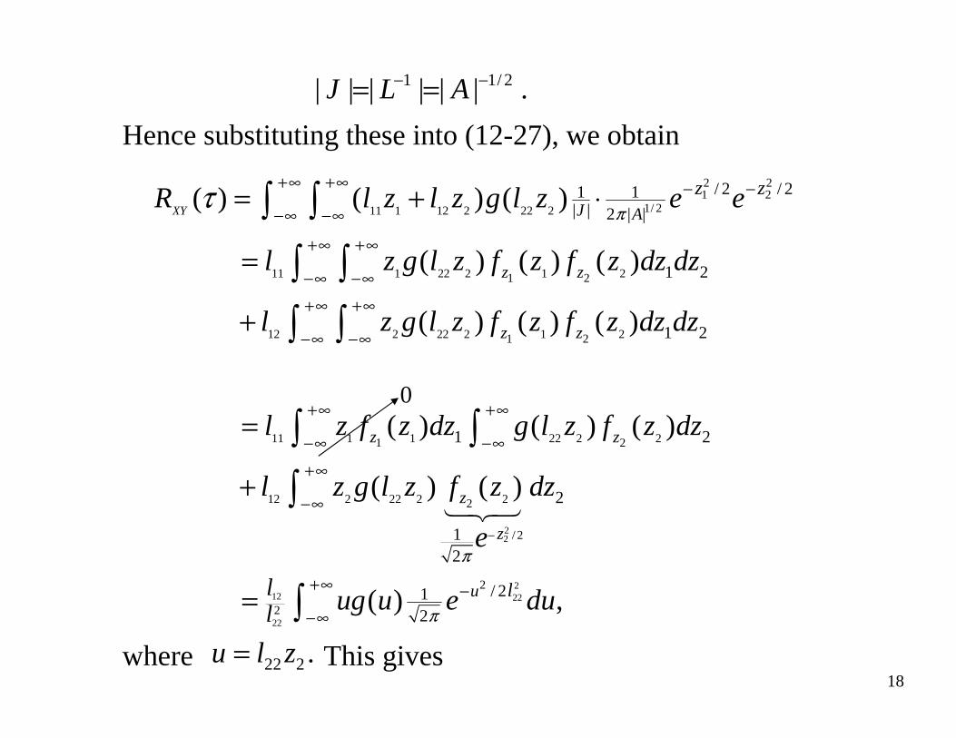
Hence substituting these into (12-27), we obtain

where This gives

.|||||| 2/11 −− == ALJ

2 21 2

1/ 211 1 12 2 22 2

11 1 22 2 1 21 2

12 2 22 2 1 21 2

/ 2 / 21 1| | 2 | |

1 2

1 2

( ) ( ) ( )

( ) ( ) ( )

( ) ( ) ( )

XY J A

z z

z z

z zR l z l z g l z e e

l z g l z f z f z dz dz

l z g l z f z f z dz dz

πτ +∞ +∞ − −

−∞ −∞

+∞ +∞

−∞ −∞+∞ +∞

−∞ −∞

= + ⋅

=

+

=

∫ ∫

∫ ∫

∫ ∫

22

212 22

22

11 1 1 22 2 21 2

12 2 22 2 22

/ 2

2

2

1 2

2

12

/ 212

( ) ( ) ( )

( ) ( )

( ) ,

z z

z

z

u lll

l z f z dz g l z f z dz

l z g l z f z dz

e

ug u e du

π

π

−

+∞ +∞

−∞ −∞+∞

−∞

+∞ −−∞

+

=

∫ ∫

∫

∫

0

22 2 .u l z=

19

222

222 22

2

2

( )

/ 2112 22 2

( )( )

( ) ( )

( ) ( ) ( ) ,

u

XY

uu

XX

f u

u

df uf u

du

u

l

lulR l l g u e du

R g u f u du

πτ

τ

+∞ −−∞

′− =−

+∞

−∞

=

′= −

∫

∫

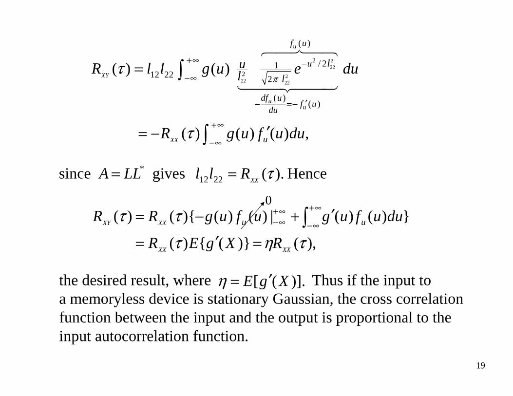
Hence).( gives since 2212* τ

XXRllLLA ==

the desired result, where Thus if the input to a memoryless device is stationary Gaussian, the cross correlation function between the input and the output is proportional to theinput autocorrelation function.

),()}({)(

})()(|)()(){()(

τητ

ττ

XXXX

XXXY

RXgER

duufugufugRR uu

=′=

′+−= ∫∞+

∞−∞+∞−

0

)].([ XgE ′=η

20

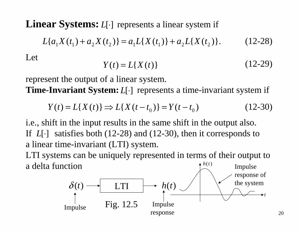
Linear Systems: represents a linear system if

Let

represent the output of a linear system.Time-Invariant System: represents a time-invariant system if

i.e., shift in the input results in the same shift in the output also.If satisfies both (12-28) and (12-30), then it corresponds to a linear time-invariant (LTI) system.LTI systems can be uniquely represented in terms of their output to a delta function

][⋅L

)}({)( tXLtY =

)}.({)}({)}()({ 22112211 tXLatXLatXatXaL +=+ (12-28)

][⋅L

)()}({)}({)( 00 ttYttXLtXLtY −=−⇒=

(12-29)

(12-30)

][⋅L

LTI)(tδ )(th

Impulse

Impulseresponse ofthe system

t

)(th

Impulseresponse

Fig. 12.5

21

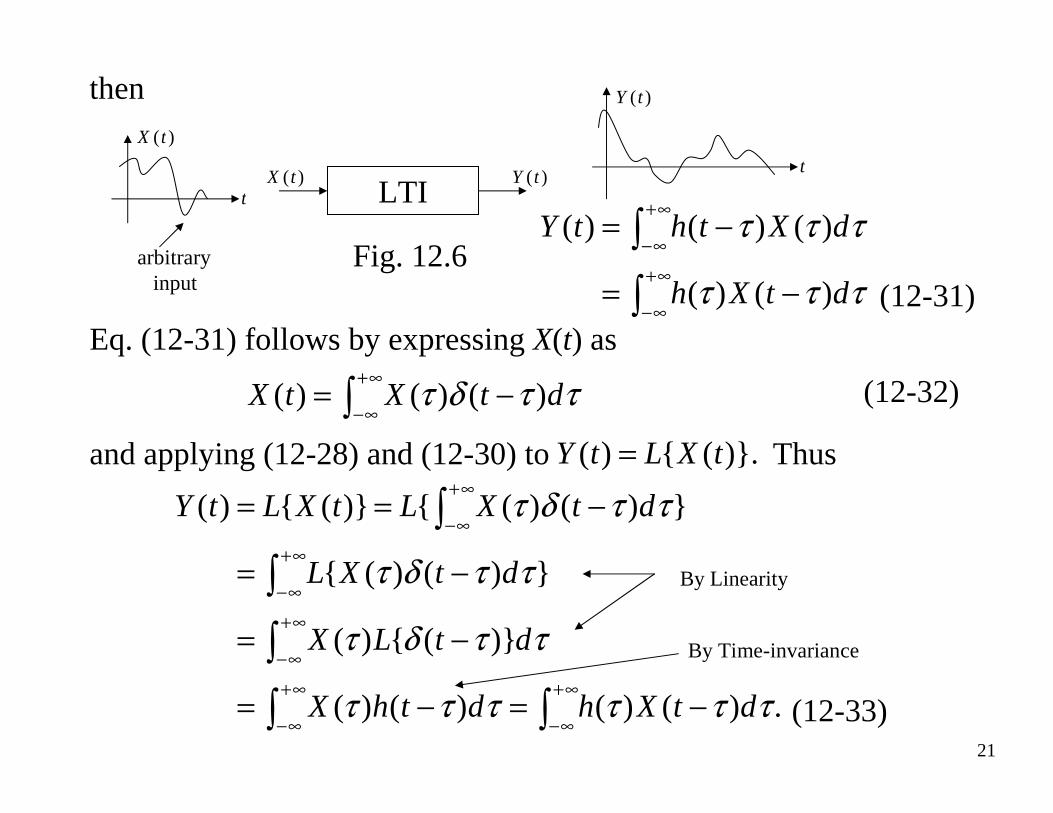
Eq. (12-31) follows by expressing X(t) as

and applying (12-28) and (12-30) to Thus)}.({)( tXLtY =∫

∞+

∞−−=

)()()( ττδτ dtXtX

(12-31)

(12-32)

(12-33).)()()()(

)}({)(

})()({

})()({)}({)(

∫∫

∫

∫

∫

∞+

∞−

∞+

∞−

∞+

∞−

∞+

∞−

∞+

∞−

−=−=

−=

−=

−==

ττττττ

ττδτ

ττδτ

ττδτ

dtXhdthX

dtLX

dtXL

dtXLtXLtY

By Linearity

By Time-invariance

then

LTI

∫

∫∞+

∞−

∞+

∞−

−=

−=

)()(

)()()(

τττ

τττ

dtXh

dXthtYarbitrary

input

t

)(tX

t

)(tY

Fig. 12.6

)(tX )(tY

22

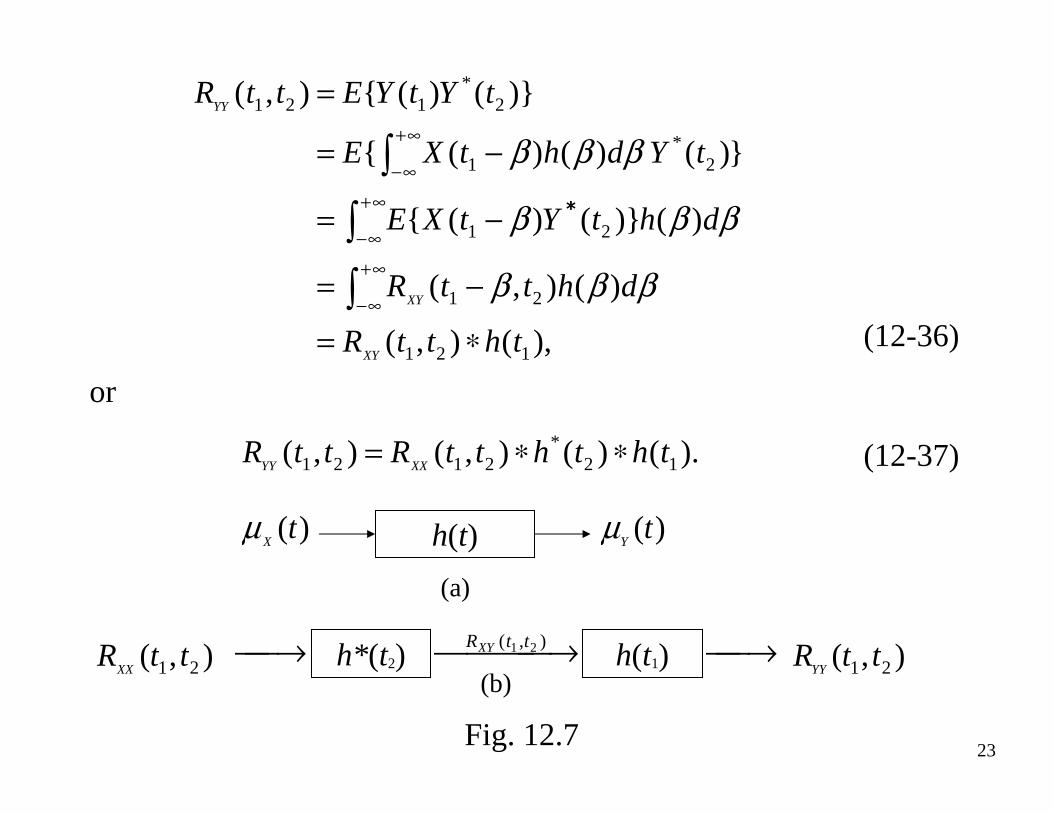
Output Statistics: Using (12-33), the mean of the output processis given by

Similarly the cross-correlation function between the input and outputprocesses is given by

Finally the output autocorrelation function is given by

).()()()(

})()({)}({)(

thtdth

dthXEtYEt

XX

Y

∗=−=

−==

∫

∫∞+

∞−

∞+

∞−

µτττµ

τττµ

(12-34)

).(),(

)(),(

)()}()({

})()()({

)}()({),(

2*

21

*21

*21

*21

2*

121

thttR

dhttR

dhtXtXE

dhtXtXE

tYtXEttR

XX

XX

XY

∗=

−=

−=

−=

=

∫

∫

∫

∞+

∞−

∞+

∞−

∞+

∞−

ααα

ααα

ααα*

*

(12-35)

23

or

),(),(

)(),(

)()}()({

})( )()({

)}()({),(

121

21

21

2*

1

2*

121

thttR

dhttR

dhtYtXE

tYdhtXE

tYtYEttR

XY

XY

YY

∗=

−=

−=

−=

=

∫

∫

∫

∞+

∞−

∞+

∞−

∞+

∞−

βββ

βββ

βββ*

).()(),(),( 12*

2121 ththttRttRXXYY

∗∗=

(12-36)

(12-37)

h(t))(tX

µ )(tY

µ

h*(t2) h(t1)⎯⎯⎯ →⎯ ),( 21 ttRXY⎯→⎯ ⎯→⎯ ),( 21 ttRYY

),( 21 ttRXX

(a)

(b)

Fig. 12.7

24

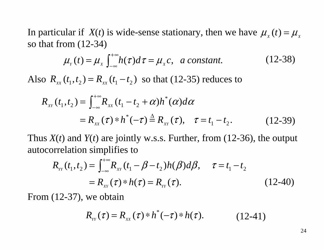
In particular if X(t) is wide-sense stationary, then we haveso that from (12-34)

Also so that (12-35) reduces to

Thus X(t) and Y(t) are jointly w.s.s. Further, from (12-36), the output autocorrelation simplifies to

From (12-37), we obtain

XXt µµ =)(

constant.a cdhtXXY

,)()(

µττµµ == ∫

∞+

∞−(12-38)

)(),( 2121 ttRttRXXXX

−=

(12-39)

).()()(

,)()(),( 21

2121

τττ

τβββ

YYXY

XYYY

RhR

ttdhttRttR

=∗=

−=−−= ∫∞+

∞−

(12-40)

).()()()( * ττττ hhRRXXYY

∗−∗= (12-41)

. ),()()(

)()(),(

21*

*2121

ttRhR

dhttRttR

XYXX

XXXY

−==−∗=

+−= ∫∞+

∞−

ττττ

ααα∆

25

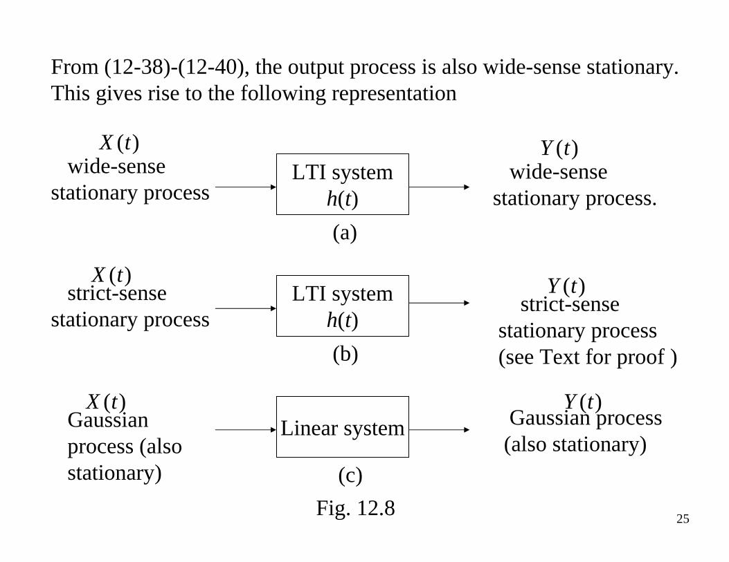
From (12-38)-(12-40), the output process is also wide-sense stationary.This gives rise to the following representation

LTI systemh(t)

Linear system

wide-sense stationary process

strict-sense stationary process

Gaussianprocess (alsostationary)

wide-sense stationary process.

strict-sensestationary process(see Text for proof )

Gaussian process(also stationary)

)(tX )(tY

LTI systemh(t)

)(tX

)(tX

)(tY

)(tY

(a)

(b)

(c)

Fig. 12.8

26

White Noise Process:W(t) is said to be a white noise process if

i.e., E[W(t1) W*(t2)] = 0 unless t1 = t2.W(t) is said to be wide-sense stationary (w.s.s) white noise if E[W(t)] = constant, and

If W(t) is also a Gaussian process (white Gaussian process), then all of its samples are independent random variables (why?).

For w.s.s. white noise input W(t), we have

),()(),( 21121 tttqttRWW

−= δ (12-42)

).()(),( 2121 τδδ qttqttRWW

=−= (12-43)

White noiseW(t)

LTIh(t)

Colored noise

( ) ( ) ( )N t h t W t= ∗

Fig. 12.9

27

and

where

Thus the output of a white noise process through an LTI system represents a (colored) noise process.Note: White noise need not be Gaussian.

“White” and “Gaussian” are two different concepts!

)()()(

)()()()(*

*

τρτττττδτ

qhqh

hhqRnn

=∗−=

∗−∗=(12-45)

.)()()()()(

** ∫∞+

∞−+=−∗= αταατττρ dhhhh (12-46)

(12-44)

[ ( )] ( ) ,

WE N t h dµ τ τ+∞

−∞= ∫ a constant