people.inf.ethz.chpeople.inf.ethz.ch/arbenz/ewp/slides/slides12.pdf · · 2016-05-17lecture 12,...

Solving large scale eigenvalue problems

Solving large scale eigenvalue problemsLecture 12, May 16, 2018: Rayleigh quotient minimization

http://people.inf.ethz.ch/arbenz/ewp/

Peter ArbenzComputer Science Department, ETH Zurich

E-mail: [email protected]

Large scale eigenvalue problems, Lecture 12, May 16, 2018 1/37

http://people.inf.ethz.ch/arbenz/ewp/


Survey

Survey of today’s lecture

I Rayleigh quotient minimization

I Method of steepest descent

I Conjugate gradient algorithm

I Preconditioned conjugate gradient algorithm

I Locally optimal PCG (LOPCG)

I Locally optimal block PCG (LOBPCG)



Rayleigh quotient

Rayleigh quotient

We consider symmetric/Hermitian eigenvalue problem

Ax = λMx , A = A∗, M = M∗ > 0.

The Rayleigh quotient is defined as

ρ(x) =x∗Ax

x∗Mx.

We want to exploit that

λ1 = minx 6=0

ρ(x) (1)

andλk = min

Sk⊂Rnmaxx 6=0x∈Sk

ρ(x)

where Sk is a subspace of dimension k .Large scale eigenvalue problems, Lecture 12, May 16, 2018 3/37


Rayleigh quotient

Rayleigh quotient minimization

Want to construct sequence {xk}k=0,1,... such that

ρ(xk+1) < ρ(xk) for all k .

The hope is that the sequence {ρ(xk)} converges to λ1 and byconsequence the vector sequence {xk} towards the correspondingeigenvector.Procedure: For any given xk we choose a search direction pk s.t.

xk+1 = xk + δkpk .

Parameter δk determined s.t. Rayleigh quotient of xk+1 is minimal:

ρ(xk+1) = minδρ(xk + δpk).



Rayleigh quotient

Rayleigh quotient minimization (cont.)

ρ(xk + δpk) =x∗kAxk + 2δx∗kApk + δ2p∗kApkx∗kMxk + 2δx∗kMpk + δ2p∗kMpk

=

(1δ

)∗ [x∗kAxk x∗kApkp∗kAxk p∗kApk

](1δ

)(

1δ

)∗ [x∗kMxk x∗kMpkp∗kMxk p∗kMpk

](1δ

) .This is Rayleigh quotient associated with eigenvalue problem[

x∗kAxk x∗kApkp∗kAxk p∗kApk

](αβ

)= λ

[x∗kMxk x∗kMpkp∗kMxk p∗kMpk

](αβ

). (2)

Smaller of the two eigenvalues of (2) is the searched valueρk+1 := ρ(xk+1) that minimizes the Rayleigh quotient.



Rayleigh quotient

Rayleigh quotient minimization (cont.)We normalize corresponding eigenvector such that its firstcomponent equals one. (Is this always possible?)Second component of eigenvector is δ = δk .Second line of (2) gives

p∗kA(xk + δkpk) = ρk+1p∗kM(xk + δkpk)

orp∗k(A− ρk+1M)(xk + δkpk) = p∗krk+1 = 0. (3)

‘Next’ residual rk+1 is orthogonal to actual search direction pk .

How shall we choose the search directions pk?



The method of steepest descent

Detour: steepest descent method for linear systems

We consider linear systems

Ax = b, (4)

where A is SPD (or HPD). We define the functional

ϕ(x) ≡ 1

2x∗Ax − x∗b +

1

2b∗A−1b =

1

2(Ax − b)∗A−1(Ax − b).

ϕ is minimized (actually zero) at the solution x∗ of (4). Thenegative gradient of ϕ is

−∇ϕ(x) = b − Ax =: r(x). (5)

This is the direction in which ϕ decreases the most. Clearly,∇ϕ(x) 6= 0 ⇐⇒ x 6= x∗.




Steepest descent method for eigenvalue problem

We choose pk to be the negative gradient of the Rayleigh quotient

pk = −gk = −∇ρ(xk) = − 2

x∗kMxk(Axk − ρ(xk)Mxk).

Since we only care about directions we can equivalently set

pk = rk = Axk − ρkMxk , ρk = ρ(xk).

With this choice of search direction we have from (3)

r∗k rk+1 = 0. (6)

The method of steepest descent often converges slowly, as forlinear systems. This happens if the spectrum is very much spreadout, i.e., if the condition number of A relative to M is big.




Slow convergence of steepest descent method

Picture: M. Gutknecht



The conjugate gradient algorithm

Detour: Conjugate gradient algorithm for linear systems

As with linear systems of equations a remedy against the slowconvergence of steepest descent are conjugate search directions.In the cg algorithm, we define search directions as

pk = −gk + βkpk−1, k > 0. (7)

where coefficient βk is determined s.t. pk and pk−1 are conjugate:

p∗kApk−1 = −g∗kApk−1 + βkp∗k−1Apk−1 = 0,

So,

βk =g∗kApk−1p∗k−1Apk−1

= · · · =g∗k gk

g∗k−1gk−1. (8)

One can show that p∗kApj = g∗k gj = 0 for j < k .





The conjugate gradient algorithm can be adapted to eigenvalueproblems.

The idea is straightforward: consecutive search directions mustsatisfy p∗kApk−1 = 0.

The crucial difference to linear systems stems from the fact, thatthe functional that is to be minimized, i.e., the Rayleigh quotient,is not quadratic anymore. (E.g., there is no finite terminationproperty.)

The gradient of ρ(x) is

g = ∇ρ(xk) =2

x∗Mx(Ax − ρ(x)Mx).




The conjugate gradient algorithm (cont.)In the case of eigenvalue problems the different expressions for βkin (7)–(8) are not equivalent anymore. We choose

p0 = −g0, k = 0,

pk = −gk +g∗kMgk

g∗k−1Mgk−1pk−1, k > 0,

(9)

which is the best choice according to Feng and Owen [1].

The above formulae is for the generalized eigenvalue problemAx = λMx .




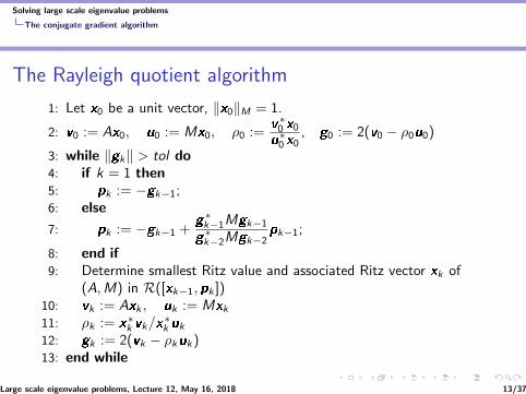
The Rayleigh quotient algorithm

1: Let x0 be a unit vector, ‖x0‖M = 1.

2: v0 := Ax0, u0 := Mx0, ρ0 :=v∗0 x0u∗0 x0

, g0 := 2(v0 − ρ0u0)

3: while ‖gk‖ > tol do4: if k = 1 then5: pk := −gk−1;6: else

7: pk := −gk−1 +g∗k−1Mgk−1

g∗k−2Mgk−2

pk−1;

8: end if9: Determine smallest Ritz value and associated Ritz vector xk of

(A,M) in R([xk−1,pk ])10: vk := Axk , uk := Mxk11: ρk := x∗

k vk/x∗k uk

12: gk := 2(vk − ρkuk)13: end while




Convergence

Construction of algorithm guarantees that ρ(xk+1) < ρ(xk) unlessrk = 0, in which case xk is the searched eigenvector.

In general, i.e., if the initial vector x0 has a nonvanishingcomponent in the direction of the ‘smallest’ eigenvector u1,convergence is toward the smallest eigenvalue λ1.

Letxk = cosϑku1 + sinϑkzk =: cosϑku1 + wk , (10)

where ‖xk‖M = ‖u1‖M = ‖zk‖M = 1 and u∗1Mzk = 0. Then wehave

ρ(xk) = cos2 ϑkλ1 + 2 cosϑk sinϑku∗1Azk + sin2 ϑkz

∗kAzk

= λ1(1− sin2 ϑk) + sin2 ϑkρ(zk),




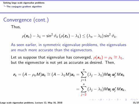
Convergence (cont.)Thus,

ρ(xk)− λ1 = sin2 ϑk (ρ(zk)− λ1) ≤ (λn − λ1) sin2 ϑk .

As seen earlier, in symmetric eigenvalue problems, the eigenvaluesare much more accurate than the eigenvectors.

Let us suppose that eigenvalue has converged, ρ(xk) = ρk ∼= λ1,but the eigenvector is not yet as accurate as desired. Then,

rk = (A− ρkM)xk ∼= (A− λ1M)xk =n∑

j=1

(λj − λ1)Muj u∗j Mxk

=n∑

j=2

(λj − λ1)Muj u∗j Mxk ,




Convergence (cont.)Therefore, u∗1 rk = 0. From (10) we have wk = sinϑkzk ⊥M u1.Thus, {

(A− λ1M)wk = (A− λ1M)xk = rk ⊥u1,

w∗kMu1 = 0.

If λ1 is a simple eigenvalue of the pencil (A;M) then A− λ1M is abijective mapping of R(u1)⊥M onto R(u1)⊥.

If rk ∈ R(u1)⊥ then the equation

(A− λ1M)wk = rk , w∗kMu1 = 0, (11)

has a unique solution wk in R(u1)⊥M .




Convergence (cont.)Close to convergence, Rayleigh quotient minimization does nothingbut solve equation (11). i.e., CG algorithm is applied to solve (11).

Convergence of RQMIN is determined by the condition number ofA− λ1M (as a mapping of R(u1)⊥M onto R(u1)⊥):

κ0 = K(A− λ1M)∣∣∣R(u1)

⊥M=λn − λ1λ2 − λ1

,

High condition number if |λ1 − λ2| � |λ1 − λn|.Rate of convergence: √

κ0 − 1√κ0 + 1

.




Preconditioning

We try to turnAx = λMx

intoAx = λM x ,

such that

κ(A− λ1M)∣∣∣R(u1)

⊥M� κ(A− λ1M)

∣∣∣R(u1)

⊥M.

Change of variables: y = Cx with C nonsingular

ρ(x) =x∗Ax

x∗Mx=

y∗C−∗AC−1y

y∗C−∗MC−1y=

y∗Ay

y∗My= ρ(y)




Preconditioning (cont.)Thus,

A− λ1M = C−∗(A− λ1M)C−1,

or, after a similarity transformation,

C−1(A− λ1M)C = (C ∗C )−1(A− λ1M).

How should we choose C to satisfy (18)?

Let us tentatively set C ∗C = A. Then

(C ∗C )−1(A− λ1M)uj = (I − λ1A−1M)uj =

(1− λ1

λj

)uj .

Note that

0 ≤ 1− λ1λj

< 1.




Preconditioning (cont.)The ‘true’ condition number of the modified problem is

κ1 := κ(A−1(A− λ1M)

∣∣R(u1)

⊥M

)=

1− λ1λn

1− λ1λ2

=λ2λn

λn − λ1λ2 − λ1

=λ2λnκ0.

If λ2 � λn then condition number is much reduced. Further,

κ1 =1− λ1/λn1− λ1/λ2

.1

1− λ1/λ2.

In FE applications, κ1 does not dependent on mesh-width h.

Conclusion: choose C such that C ∗C ∼= A, e.g. IC(0).




Preconditioning (cont.)Transformation x −→ y = Cx need not be made explicitly.

In the code of page 12 we modify the computation of the gradientgk .

Statement 12 becomes

gk = 2(C ∗C )−1(vk − ρkuk)

Then preconditioner need not be an (incomplete) factorizationof A.



Locally optimal PCG (LOPCG)


Parameters δk and αk in RQMIN and (P)CG:

ρ(xk+1) = ρ(xk + δkpk), pk = −gk + αkpk−1

The parameters are determined such that ρ(xk+1) is minimizedand consecutive search directions are conjugate.

Knyazev [2]: optimize both parameters, αk and δk , at once

ρ(xk+1) = minδ,γ

ρ(xk − δgk + γpk−1) (12)

Results in potentially smaller values for the Rayleigh quotient, as

minδ,γ

ρ(xk − δgk + γpk−1

)≤ min

δ

(xk − δ(gk − αkpk)

).

Procedure is “locally optimal”.Large scale eigenvalue problems, Lecture 12, May 16, 2018 22/37



Locally optimal PCG (LOPCG) (cont.)ρ(xk+1) in (12) is minimal eigenvalue of 3× 3 eigenvalue problem x∗k−g∗kp∗k−1

A[xk ,−gk ,pk−1]

αβγ

= λ

x∗k−g∗kp∗k−1

M[xk ,−gk ,pk−1]

αβγ

We normalize eigenvector such that first component is 1:

[1, δk , γk ] := [1, β/α, γ/α].

Then

xk+1 = xk−δkgk+γkpk−1 = xk+δk (−gk + (γk/δk)pk−1)︸︷︷︸=:pk

= xk+δkpk .

RQ minimization from xk along pk = −gk + (γk/δk)pk−1.



Comparison

Test: car cross section: 1st eigenvalue



Block versions

Block versions

Above procedures converge very slowly if eigenvalues are clustered.

Hence, these methods should be applied only in blocked form.

BRQMIN: Rayleigh quotient is minimized in 2q-dimensionalsubspace generated by the eigenvector approximations Xk andsearch directions

Pk = −Hk + Pk−1Bk .

Hk : preconditioned residualsBk chosen such that the block of search directions is conjugate.

LOBPCG: Similar as BRQMIN, but search space is 3qdimensional: R([Xk ,Hk ,Pk−1]).



Block versions

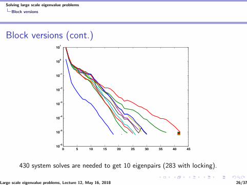
Block versions (cont.)

0 5 10 15 20 25 30 35 40 4510

−6

10−5

10−4

10−3

10−2

10−1

100

101

430 system solves are needed to get 10 eigenpairs (283 with locking).



Trace minimization

Trace minimization

Theorem

(Trace theorem for the generalized eigenvalue problem) LetA = A and M be as in (3). Then,

λ1 + λ2 + · · ·+ λp = minX∈Fn×p , X∗MX=Ip

trace(X ∗AX ) (13)

where λ1, . . . , λn are the eigenvalues of problem (3). Equalityholds in (13) if and only if the columns of the matrix X thatachieves the minimum span the eigenspace corresponding to thesmallest p eigenvalues.

Let’s try to use the theorem to derive an algorithm.



Trace minimization

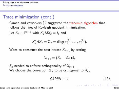
Trace minimization (cont.)Sameh and coworkers [3] suggested the tracemin algorithm thatfollows the lines of Rayleigh quotient minimization.

Let Xk ∈ Fn×p with X ∗kMXk = Ip and

X ∗kAXk = Σk = diag(σ(k)1 , . . . , σ

(k)p ).

Want to construct the next iterate Xk+1 by setting

Xk+1 = (Xk −∆k)Sk

Sk needed to enforce orthogonality of Xk+1.We choose the correction ∆k to be orthogonal to Xk ,

∆∗kMXk = 0. (14)



Trace minimization

Trace minimization (cont.)Want to minimize

trace((Xk −∆k)∗A(Xk −∆k)) =

p∑i=1

e∗i (Xk −∆k)∗A(Xk −∆k)ei

=

p∑i=1

(xi − di )∗A(xi − di )

with xi = Xkei and di = ∆kei .

These are p individual minimization problems:

Minimize (xi−di )∗A(xi−di ) subject to X ∗kMdi = 0, i = 1, . . . , p.

To solve this eq. we define the functional

f (d , l ) := (xi − d )∗A(xi − d ) + l ∗X ∗kMd .



Trace minimization

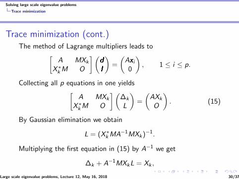
Trace minimization (cont.)The method of Lagrange multipliers leads to[

A MXk

X ∗kM O

](d

l

)=

(Axi

0

), 1 ≤ i ≤ p.

Collecting all p equations in one yields[A MXk

X ∗kM O

](∆k

L

)=

(AXk

O

). (15)

By Gaussian elimination we obtain

L = (X ∗kMA−1MXk)−1.

Multiplying the first equation in (15) by A−1 we get

∆k + A−1MXkL = Xk ,



Trace minimization

Trace minimization (cont.)So,

Zk+1 ≡ Xk −∆k = A−1MXkL = A−1MXk(X ∗kMA−1MXk)−1.

such that, one step of the above trace minimization algorithmamounts to one step of subspace iteration with shift σ = 0.

This implies convergence. Bit requires factorization of A.

Rewrite saddle point problem (15) as a simple linear problem,which can be solved iteratively.



Trace minimization

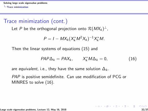
Trace minimization (cont.)Let P be the orthogonal projection onto R(MXk)⊥,

P = I −MXk(X ∗kM2Xk)−1X ∗kM.

Then the linear systems of equations (15) and

PAP∆k = PAXk , X ∗kM∆k = 0, (16)

are equivalent, i.e., they have the same solution ∆k .

PAP is positive semidefinite. Can use modification of PCG orMINRES to solve (16).



Trace minimization

Tricks of the trade

I Simple shifts. Choose a shift σ1 ≤ λ1 until the first eigenpairis found. Then proceed with the shift σ2 ≤ λ2 and lock thefirst eigenvector. In this way PCG can be used to solve thelinear systems as before.

I Multiple dynamic shifts. Each linear system

P(A− σ(k)i M)Pd(k)i = Pri , d

(k)i ⊥M Xk

is solved with an individual shift. The shift is ‘turned on’ closeto convergence. Systems indefinite ⇒ PCG has to be adapted.

I Preconditioning. Systems above can be preconditioned, e.g.,by a matrix of the form M = CC ∗ where CC ∗ ≈ A is anincomplete Cholesky factorization.



Trace minimization

The Tracemin algorithm

1: Choose matrix V1 ∈ Rn×q with V T1 MV1 = Iq, q ≥ p.

2: for k = 1, 2, . . . until convergence do3: Compute Wk = AVk and Hk := V ∗

k Wk .4: Compute spectral decomposition Hk = UkΘkU

∗k ,

with Θk = diag(ϑ(k)1 , . . . , ϑ

(k)q ), ϑ

(k)1 ≤ . . . ≤ ϑ

(k)q .

5: Compute Ritz vectors Xk = VkUk and residualsRk = WkUk −MXkΘk

6: For i = 1, . . . , q solve approximatively

P(A− σ(k)i M)Pd

(k)i = Pri , d

(k)i ⊥M Xk

by some modified PCG solver.

7: Compute Vk+1 = (Xk −∆k)Sk , ∆k = [d(k)1 , . . . ,d

(k)q ], by a

M-orthogonal modified Gram-Schmidt procedure.8: end for



Trace minimization

Numerical experiment (from [3])

Problem Size Max # Block Jacobi–Davidson Davidson-type Tracemininner its #its A mults time[sec] #its A mults time[sec]

BCSST08 1074 40 34 3954 4.7 10 759 0.8BCSST09 1083 40 15 1951 2.2 15 1947 2.2BCSST11 1473 100 90 30990 40.5 54 20166 22.4BCSST21 3600 100 40 10712 35.1 39 11220 36.2BCSST26 1922 100 60 21915 32.2 39 14102 19.6

Table 1: Numerical results for problems from the Harwell–Boeingcollection with four processors.IC(0) of A was used as preconditioner.Davidson-type trace minimization algorithm with multiple dynamic shiftsworks better than block Jacobi–Davidson for three out of five problems.



References

References

[1] Y. T. Feng and D. R. J. Owen. Conjugate gradient methods for solvingthe smallest eigenpair of large symmetric eigenvalue problems, Internat. J.Numer. Methods Eng., 39 (1996), pp. 2209–2229.

[2] A. V. Knyazev. Toward the optimal preconditioned eigensolver: Locallyoptimal block preconditioned conjugate gradient method, SIAM J. Sci.Comput., 23 (2001), pp. 517–541.

[3] A. Sameh and Z. Tong. The trace minimization method for the symmetricgeneralized eigenvalue problem, J. Comput. Appl. Math., 123 (2000),pp. 155–175.

[4] A. Klinvex, F. Saied, and A. Sameh. Parallel implementations of the traceminimization scheme TraceMIN for the sparse symmetric eigenvalueproblem, Comput. Math. Appl., 65(3):460–468, 2013.



The end


people.inf.ethz.chpeople.inf.ethz.ch/arbenz/ewp/slides/slides12.pdf · · 2016-05-17lecture 12,...

Documents